Stationary solutions for the 2D critical Dirac equation with Kerr nonlinearity

Abstract

In this paper we prove the existence of an exponentially localized stationary solution for a two-dimensional cubic Dirac equation. It appears as an effective equation in the description of nonlinear waves for some Condensed Matter (Bose-Einstein condensates) and Nonlinear Optics (optical fibers) systems. The nonlinearity is of Kerr-type, that is of the form $|\psi|^{2}\psi$ and thus not Lorenz-invariant. We solve compactness issues related to the critical Sobolev embedding $H^{\frac{1}{2}}(\mathbb{R}^{2},\mathbb{C}^{2})\hookrightarrow L^{4}(\mathbb{R}^{2},\mathbb{C}^{4})$ thanks to a particular radial ansatz. Our proof is then based on elementary dynamical systems arguments.

Introduction

The Dirac equation has been widely used to build relativistic models of particles(see the survey paper [1]).

Recently, it made its appearance in Condensed Matter Physics. New two-dimensional materials possessing Dirac fermions as low-energy excitations have been discovered, the most famous being the graphene [2] (2010 Nobel Prize in Physics awarded to A.Geim and K. Novoselov). Those Dirac materials, possess unique electronic properties which are consequence of the Dirac spectrum. They range from superfluid phases of ³He, high-temperature d-wave superconductors, graphene to topological insulators (see [3, 4, 5] and references therein). Particular symmetries control the appearance of Dirac points. Time-reversal symmetry in topological insulators and sublattice symmetry in graphene [5] are some examples. In the paper [6] the authors rigorously proved existence and stability of Dirac cones for honeycomb Schrödinger operators, under fairly general assumptions.

The possibility of finding three-dimensional materials exhibiting a Dirac spectrum has also recently gained attention in the Physics community [3].

In contrast to the case of many metals and doped semi-conductors, where nearly free quasi-particles obeying the Schrödinger equation with an effective mass represent a very accurate approximation for low energy-excitations, for Dirac materials an accurate description is provided by the Dirac hamiltonian

$$H=-iv_{F}(\vec{\sigma}\cdot\nabla)+mv_{F}^{2}\sigma_{3}$$

where the speed of light is replaced by the Fermi velocity $v_{F}$ and $m$ is an effective mass.

If $m=0$ the dispersion relation is linear (i.e. a cone), in contrast with the parabolic dispersion of metals or semiconductors. This case includes graphene monolayers [5].

The case of a non-vanishing mass term ($m\neq 0$) corresponds to a gap at the Fermi level. It describes, for instance, a monolayer of boron-nitride or graphene bilayers ([4]). It has been experimentally proved that placing boron-nitride in contact with graphene leads to the appearance of a non-zero mass, thus creating an energy gap.

Furthermore, using arguments from [7] and [8] a multiscale expansion shows that applying a suitable electric field (formally) opens a gap in the effective Dirac hamiltonian for the graphene, in the case of wavefunctions spectrally concentrated around a Dirac point. In the recent paper [8] the authors showed the existence of a gap for honeycomb Schrödinger operators in the strong-binding regime, when an electric potential that breaks the $\mathcal{PT}$-symmetry (parity+time-inversion) is applied.

An important model in nonlinear optics and in the description of macroscopic quantum phenomena (see [9],[10]) is the cubic Schrödinger / Gross-Pitaevskii equation:

$$i\partial_{t}\Psi=\left(-\Delta+V\right)\Psi+g|\Psi|^{2}\Psi$$ (1)

where $g$ is a parameter that measures the scattering length and the cubic term is a mean field interaction or a Kerr-nonlinear term due to a variable refractive index, according to the model.

The above equation appears, for instance, in the description of Bose-Einstein condensates.

If $V$ is a honeycomb potential, the low-energy effective operator around a Dirac point is the Dirac operator (see [5]) :

$$\left(-\Delta+V\right)\longmapsto\mathcal{D}:=-ic\left(\vec{\sigma}\cdot\nabla\right)$$ (2)

Note that it acts on two-components spinors

$$\psi=\begin{pmatrix}\psi^{1}\\ \psi^{2}\end{pmatrix}\in\mathbb{C}^{2}$$

since the honeycomb lattice is a superposition of two triangular Bravais lattices. In this case the spinor encodes the isospin of the sublattices, rather than the proper spin of the electron (see [5]).

As remarked above, applying a suitable electric potential or placing the material on a substrate results in an additional mass term. Thus the effective equation reads as

$$i\partial_{t}\Psi=\left(\mathcal{D}+m\sigma_{3}\right)\Psi+g|\Psi|^{2}\Psi$$ (3)

Our aim is to prove the existence of stationary solutions to (3) in the focusing case, $g=-1$. Setting

$$\Psi(x,t)=e^{-i\omega t}\psi(x)$$

with $0<\omega<m$, the equation rewrites as

$$\left(\mathcal{D}+m\sigma_{3}-\omega\right)\psi-|\psi|^{2}\psi=0$$ (4)

The main result of this paper is the following

Theorem 1.

Equation (4) admits a smooth localized solution, with exponential decay at infinity.

Remark 2.

The result presented here is at odds with the case of the pseudo-relativistic operator

$$\sqrt{-\Delta+m^{2}}\geqslant 0$$

Indeed, a simple Pohozaev-type argument shows that there is no smooth exponentially localized solution to the following equation

$$\left(\sqrt{-\Delta+m^{2}}\right)\psi-\omega\psi=|\psi|^{2}\psi\qquad\mbox{on}\quad\mathbb{R}^{2}$$ (5)

with $0<\omega<m$.

Thus the existence of solutions is related to the presence of the negative part of the spectrum of the Dirac operator (see next section).

Remark 3.

In this case the zero-energy corresponds to the Fermi level. Then there is no interpretation of the Dirac spectrum in terms of particles/antiparticles. Rather, the positive part of the spectrum corresponds to massive conduction electrons, while the negative one to valence electrons.

Acknowledgment. The author wishes to thank Éric Séré for his support.

1 Preliminaries

The Dirac operator is a first order differential operator formally defined in 2D (in the standard representation) as

$$\mathcal{D}_{m}=\mathcal{D}+mc^{2}\sigma_{3}:=-ic\hbar(\vec{\sigma}\cdot\nabla)+mc^{2}\sigma_{3}$$ (6)

where $c$ denotes the speed of light, $m$ is the electron mass, $\hbar$ is the reduced Planck constant, $\vec{\sigma}\cdot\nabla:=\sigma_{1}\partial_{1}+\sigma_{2}\partial_{2}$ and the $\sigma_{k}$ are the Pauli matrices

$$\sigma_{1}:=\begin{pmatrix}0\quad&1\\ 1\quad&0\end{pmatrix}\quad,\quad\sigma_{2}:=\begin{pmatrix}0\quad&-i\\ i\quad&0\end{pmatrix}\quad,\quad\sigma_{3}:=\begin{pmatrix}1\quad&0\\ 0\quad&-1\end{pmatrix}$$ (7)

In this paper we shall work with a system of physical units such that $c=1$ and $\hbar=1$.

It is well known (see [11]) that $\mathcal{D}_{m}$ is a self-adjoint operator on $L^{2}(\mathbb{R}^{2},\mathbb{C}^{2})$, with domain $H^{1}(\mathbb{R}^{2},\mathbb{C}^{2})$ and form-domain $H^{\frac{1}{2}}(\mathbb{R}^{2},\mathbb{C}^{2})$.

Moreover, in Fourier domain $p=(p_{1},p_{2})$ the Dirac operator becomes the multiplication operator by the matrix

$$\widehat{\mathcal{D}}_{m}(p)=\begin{pmatrix}m\quad&p_{1}-ip_{2}\\ p_{1}+ip_{2}\quad&m\end{pmatrix}$$

so the spectrum is given by

$$Spec(\mathcal{D}_{m})=(-\infty,-m]\cup[m,+\infty)$$ (8)

where the gap is due to the mass term.

In this paper we focus on the following equation

$$\left(\mathcal{D}+m\sigma_{3}-\omega\right)\psi-|\psi|^{2}\psi=0\qquad\mbox{on}\quad\mathbb{R}^{2},\quad\mbox{with}\quad 0<\omega<m$$ (9)

whose weak solutions correspond to critical points of the following functional

$$\mathcal{L}(\psi):=\frac{1}{2}\int\langle\left(\mathcal{D}+m\sigma_{3}-\omega\right)\psi,\psi\rangle-\frac{1}{4}\int|\psi|^{4}$$ (10)

defined for $\psi\in H^{\frac{1}{2}}(\mathbb{R}^{2},\mathbb{C}^{2})$.

The above functional is strongly indefinite, that is, it is unbounded both from above and below, even modulo finite dimensional subspaces. This is due to the unboundedness of $Spec(\mathcal{D})$. Several techniques have been introduced to deal with such situations (see for instance [12]).

Moreover, the main difficulty in our case is given by the lack of compactness of the Sobolev embedding $H^{\frac{1}{2}}(\mathbb{R}^{2},\mathbb{C}^{2})\hookrightarrow L^{4}(\mathbb{R}^{2},\mathbb{C}^{2})$. This implies the failure of some compactness properties used to prove linking results (see [12] and references therein), due to the invariance by translations and scaling.

In what follows we will only give a sketch of the compactness analysis for the above functional, referring to the mentioned papers for more details.

As we will see in the next section, equation (9) is compatible with a particular ansatz, leading us to work in the closed subspace

$$E=\left\{\psi\in H^{\frac{1}{2}}(\mathbb{R}^{2},\mathbb{C}^{2}):\psi(r,\vartheta)=\begin{pmatrix}v(r)\\ iu(r)e^{i\vartheta}\end{pmatrix},u,v:(0,+\infty)\rightarrow\mathbb{R}\right\}$$ (11)

where $(r,\vartheta)$ are the polar coordinates of $x\in\mathbb{R}^{2}$.

Restricting the problem to the subspace $E$ breaks the invariance by translations, and thus to recover compactness one has to deal with the invariance by scaling only. The latter causes the so-called bubbling phenomenon, that is, energy concentration associated to the appearance of blow-up profiles. In [13] Isobe analyzed the behavior of a generic Palais-Smale sequence for the critical Dirac equation on compact spin manifolds. The same can be done in our case.

Given a Palais-Smale sequence $\left(\psi_{n}\right)\subseteq H^{\frac{1}{2}}$ it easy to see that it is bounded, and thus we may suppose, up to extraction, that it weakly converges

$$\psi_{n}\rightharpoonup\psi_{\infty}\in H^{\frac{1}{2}}.$$

Generally speaking, the invariance by scaling prevents the strong convergence and we have the profile decomposition

$$\psi_{n}=\psi_{\infty}+\sum^{N}_{k=1}\omega^{k}_{n}+o(1)\qquad\mbox{in}\quad H^{\frac{1}{2}}(\mathbb{R}^{2},\mathbb{C}^{2})$$ (12)

where $N\in\mathbb{N}$ and $\omega^{k}_{n}$ is a properly rescaled $\mathring{H}^{\frac{1}{2}}(\mathbb{R}^{2},\mathbb{C}^{2})$-solution of the limit equation

$$\mathcal{D}\varphi=|\varphi|^{2}\varphi$$

centered around points $a^{k}_{n}\rightarrow a^{k}\in\mathbb{R}^{2}$, as $n\rightarrow+\infty$, for $1\leqslant k\leqslant N$.

The bubbles $\omega^{k}_{n}$ are in a finite number, since one can prove a uniform lower bound for their energy. Moreover, this implies that we have compactness only in a suitable energy range and gives a treshold value for the appearance of bubbles in min-max methods (see [12]).

Then in terms of $L^{4}$-norms, there holds

$$|\psi_{n}|^{4}dx\rightharpoonup|\psi_{\infty}|^{4}dx+\sum^{N}_{k=1}\nu_{k}\delta_{a^{k}}$$ (13)

weakly in the sense of measures. Here $\nu_{k}\geqslant 0$ and the $\delta_{a^{k}}$ are delta measures concentrated at $a^{k}$.

Morever, since we are essentially working with radial functions, it’s not hard to see that the blow-up can only occur at the origin, that is, we actually have

$$|\psi_{n}|^{4}dx\rightharpoonup|\psi_{\infty}|^{4}dx+\nu\delta_{0}$$ (14)

with $\nu\geqslant 0$ and $\delta_{0}$ being the delta concentrated at the origin.

We thus conclude that in order to recover compactness for the variational problem one should be able to control the behavior of Palais-Smale sequences near the origin.

However, our proof is based on a shooting method and thus not variational. In this case the concentration phenomenon (14) manifests itself in the difficulty of controlling the behavior of solutions of the resulting dynamical system when initial data are large. This makes the analysis quite delicate and requires a careful asymptotic expansion of the solution, after a suitable rescaling (see section 2.2).

We mention that the first rigorous existence result of stationary solutions for the Dirac equation via shooting methods is due to Cazenave and Vazquez [14], who studied the Soler model for elementary fermions. Subsequently, those methods have been used to prove the existence of excited states [15] for the Soler model and in mean field theories for nucleons (see e.g. [16],[17], [1] and references therein). We remark that a variational proof has been given by Esteban and Séré in [18], under fairly general assumptions on the self-interaction. In particular, after a suitable radial ansatz, they prove a multiplicity result exploiting the Lorentz-invariance. Remarkably, their method works without any growth assumption on the nonlinearity. However, the proof is designed to deal with the Lorentz-invariant form of the nonlinear term and is not applicable in our case. In [19] Ding and Wei proved an existence result for the 3D Dirac equation with a subcritical Kerr-type interaction. The case of a critical nonlinearity in 3D has been investigated by Ding and Ruf [20] in the semiclassical regime, using variational techniques. They take advantage of the presence of a negative potential to prove compactness properties. However, in this paper we deal with a critical Kerr nonlinearity without additional assumptions and so we need to adopt a different strategy.

2 Existence by shooting method

To begin with, we first convert the equation into a dynamical system thanks to a particular ansatz. Then we will give some qualitative properties of the flow, particularly useful in understanding the long-time behavior of the system.

Passing to polar coordinates in $\mathbb{R}^{2}$ $(x,y)\mapsto(r,\vartheta)$, the equation

$$\left(\mathcal{D}+m\sigma_{3}-\omega\right)\psi-|\psi|^{2}\psi=0$$

reads as

$$\left\{\begin{aligned} -e^{-i\vartheta}\left(i\partial_{r}+\frac{\partial_{\vartheta}}{r}\right)\psi_{2}&=\left(|\psi_{1}|^{2}+|\psi_{2}|^{2}\right)\psi_{1}-(m-\omega)\psi_{1},\\ -e^{i\vartheta}\left(i\partial_{r}-\frac{\partial_{\vartheta}}{r}\right)\psi_{1}&=-\left(|\psi_{1}|^{2}+|\psi_{2}|^{2}\right)\psi_{2}-(m+\omega)\psi_{2}.\end{aligned}\right.$$ (15)

where $\psi=\begin{pmatrix}\psi_{1}\\ \psi_{2}\end{pmatrix}\in\mathbb{C}^{2}$, and this suggests the following ansatz (see [21]):

$$\psi(r,\vartheta)=\begin{pmatrix}v(r)e^{iS\vartheta}\\ iu(r)e^{i(S+1)\vartheta}\end{pmatrix}$$ (16)

with $u$ and $v$ real-valued and $S\in\mathbb{Z}$. In the sequel, we set $S=0$.

Plugging the above ansatz into the equation one gets

$$\left\{\begin{aligned} \dot{u}+\frac{u}{r}&=(u^{2}+v^{2})v-(m-\omega)v\\ \dot{v}&=-(u^{2}+v^{2})u-(m+\omega)u\end{aligned}\right.$$ (17)

Thus we are lead to study the flow of the above system.

In particular, since we are looking for localized states, we are interested in solutions to (17) such that

$$(u(r),v(r))\rightarrow(0,0)\qquad\mbox{as}\qquad r\rightarrow+\infty$$

In order to avoid singularities and to get non-trivial solutions, we choose as initial conditions

$$u(0)=0\quad,\quad v(0)=\lambda\neq 0$$

Moreover, the symmetry of the system allows us to consider only the case $\lambda>0$.

Studying the long-time behavior of the flow of (17) it is useful to introduce the following system

$$\left\{\begin{aligned} \dot{u}&=(u^{2}+v^{2})v-(m-\omega)v\\ \dot{v}&=-(u^{2}+v^{2})u-(m+\omega)u\end{aligned}\right.$$ (18)

Heuristically, (17) should reduce to (18) in the limit $r\rightarrow+\infty$ ($u$ being bounded), that is, dropping the singular term in the first equation.

As one can easily check, (18) is the hamiltonian system associated with the function

$$H(u,v)=\frac{(u^{2}+v^{2})^{2}}{4}+\frac{m}{2}(u^{2}-v^{2})+\frac{\omega}{2}(u^{2}+v^{2})$$ (19)

It’s easy to see that the level sets of the hamiltonian

$$\left\{H(u,v)=c\right\}$$

are compact, for all $c\in\mathbb{R}$, so that the flow is globally defined.

The equilibria of the hamiltonian flow are the points

$$(0,0),(0,\pm\sqrt{m-\omega})$$ (20)

and there holds

$$H(0,0)=0,\quad H(0,\pm\sqrt{m-\omega})<0$$ (21)

Local existence and uniqueness of solutions of (17) are guaranteed by the following

Lemma 4.

Let $\lambda>0$. There exist $0<R_{\lambda}\leqslant+\infty$ and $(u,v)\in C^{1}([0,R_{\lambda}),\mathbb{R}^{2})$ unique maximal solution to (17), which depends continuously on $\lambda$ and uniformly on $[0,R]$ for any $0<R<R_{\lambda}$.

Proof.

We can rewrite the system in integral form as

$$\left\{\begin{aligned} u(r)&=\frac{1}{r}\int^{r}_{0}sv(s)[u^{2}(s)+v^{2}(s)-(m-\omega)]ds\\ v(r)&=\lambda-\int^{r}_{0}u(s)[(u^{2}(s)+v^{2}(s))+(m+\omega)]ds\end{aligned}\right.$$ (22)

where the r.h.s. is a Lipschitz continuous function. Then the claim follows by a contraction mapping argument, as in [14]. ∎

Given $\lambda>0$, define

$$H_{\lambda}(r):=H(u_{\lambda}(r),v_{\lambda}(r))\quad,\quad r\in[0,R_{\lambda})$$ (23)

where $(u_{\lambda},v_{\lambda})$ is the solution of (17) such that $(u(0),v(0))=(0,\lambda)$.

A simple computation gives

$$\dot{H}_{\lambda}(r)=-\frac{u^{2}_{\lambda}}{r}(m+\omega+u^{2}_{\lambda}(r)+v^{2}_{\lambda}(r))\leqslant 0\quad,\quad\forall r\in[0,R_{\lambda})$$ (24)

so that the energy $H$ is non-increasing along the solutions of (17).

This implies that $\forall r\in[0,R_{x})$, $(u_{\lambda}(r),v_{\lambda}(r))\in\{H(u,v)\leqslant H(0,\lambda)\}$, the latter being a compact set. Thus there holds

Lemma 5.

Every solution to (17) is global.

Remark 6.

The above result is in contrast with the case of Lorentz-invariant models in 3D ([15]), where the energy has no definite sign and blow-up may occur.

The following lemma indeed shows that the solutions to (17) are close to the hamiltonian flow (18) as $r\rightarrow+\infty$. The proof is the same as the one given in [14].

Lemma 7.

Let $(f,g)$ be the solution of (18) with initial data $(f_{0},g_{0})$. Let $(u^{0}_{n},v{0}_{n})$ and $\rho_{n}$ be such that

$$\rho_{n}\xrightarrow{n\rightarrow+\infty}+\infty\qquad\mbox{and}\qquad(u_{n},v_{n})\xrightarrow{n\rightarrow+\infty}(f_{0},g_{0})$$

Consider the solution of

$$\left\{\begin{aligned} \dot{u}_{n}+\frac{u_{n}}{r+\rho_{n}}&=(u^{2}_{n}+v^{2}_{n})v_{n}-(m-\omega)v_{n}\\ \dot{v}_{n}&=-(u^{2}_{n}+v^{2}_{n})u_{n}-(m+\omega)u_{n}\end{aligned}\right.$$

such that $u_{n}(0)=u^{0}_{n}$ and $v_{n}(0)=v^{0}_{n}$.

Then $(u_{n},v_{n})$ converges to $(f,g)$ uniformly on bounded intervals.

Since we know from (24) that the energy $H_{\lambda}$ decreases along the flow of (17) and that each solution is bounded, Lemma (7) allows us to conclude (see the proof of Lemma (9)) that any solution must tend to an equilibrium of the hamiltonian flow (18). Thus a solution eventually entering the negative energy region

$$\{H(u,v)<0\}$$

will converge to

$$(0,\pm\sqrt{m-\omega})$$

spiraling toward that point. A proof of this property follows along the same lines of the analogous one given in [16]. This is illustrated by the following picture:

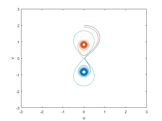
Figure 1: The energy level $\{H=0\}$ and two solutions entering the negative energy set $\{H<0\}$.

If, on the contrary, there holds

$$H_{\lambda}(r)>0,\qquad\forall r>0$$

then necessarily the solution tends to the origin, thus corresponding to a localized solution of our PDE.

2.1 The shooting method

In our proof we use some ideas from [17], [22].

Definition 1.

Put $I_{-1}=\emptyset$. For $k\in\mathbb{N}$ we define

$$A_{k} =\left\{\lambda>0:\lim_{r\rightarrow+\infty}H_{\lambda}(r)<0,v_{\lambda}\>\mbox{changes sign $k$ times on}\>(0,+\infty)\right\}$$ (25)

$$I_{k} =\left\{\lambda>0:\lim_{r\rightarrow+\infty}(u_{\lambda}(r),v_{\lambda}(r))=(0,0),v_{\lambda}\>\mbox{changes sign $k$ times on}\>(0,+\infty)\right\}.$$

It is immediate so see that

$$A_{0}\neq\emptyset$$

as it includes the interval $\left(0,\sqrt{2(m-\omega}\right]$, since

$$\{0\}\times\left(0,\sqrt{2(m-\omega)}\right]\subseteq\{(u,v)\in\mathbb{R}^{2}:H(u,v)\leqslant 0\}$$

Moreover, numerical simulations indicates that the set $A_{0}$ is bounded and that $A_{1}$ is non-empty and unbounded. This implies that $I_{0}$ is non empty (see 11). Solutions tending to the origin are expected to appear in the shooting procedure when $\lambda$ passes from $A_{k}$ to $A_{k+1}$, as in (Figure 1).

Remark 8.

We found no numerical evidence for the existence of excited states. This may lead to conjecture that there are no nodal solutions, that is $I_{k}=\emptyset$ for $k>1$. The absence of excited states is compatible with the bubbling phenomenon (see the Introduction), which might prevent the existence of those solutions. However in 3D Lorentz-invariant models ([1],[15]) it is known that they exist.

In this section we show that $I_{0}$ is non empty, thus proving (Theorem 1). This will be achieved in several intermediate steps.

We start with some preliminary lemmas, which are an adaptation of analogous results from [17].

Lemma 9.

Let $(u_{\lambda},v_{\lambda})$ be a solution of (17) such that $v_{\lambda}$ changes sign a finite number of times and

$$\lim_{r\rightarrow+\infty}H_{\lambda}(r)\geqslant 0$$

then

$$|u_{\lambda}(r)|+|v_{\lambda}(r)|\leqslant Ce^{-\left(\frac{m-\omega}{2}\right)r}\quad,\quad\forall r\geqslant 0$$ (26)

and thus

$$\lim_{r\rightarrow+\infty}(u_{\lambda}(r),v_{\lambda}(r))=(0,0)$$

Proof.

We start by showing that under the above assumptions there exists $\overline{R}\in(0,+\infty)$ such that

$$u_{\lambda}(r)v_{\lambda}(r)>0\quad,\quad\forall r\geqslant\overline{R}$$ (27)

Since $v_{\lambda}$ changes sign a finite number of times, we may suppose w.l.o.g. that for some $R>0$

$$v_{\lambda}(r)>0\quad,\quad\forall r\geqslant R$$

We have to prove that $\exists R<\overline{R}<+\infty$ such that

$$u_{\lambda}(r)>0\quad,\quad\forall r\geqslant\overline{R}$$

Assume, by contradiction, that

$$u_{\lambda}(r)<0\quad,\quad\forall r>R$$

Then the second equation of (17) implies that $\dot{v}_{\lambda}(r)>0,\forall r>R$, and $v_{\lambda}$ is increasing for $r>R$. Thus

$$\lim_{r\rightarrow+\infty}v_{\lambda}(r)=\delta\in(0,+\infty]$$

Indeed, we cannot have $\delta=+\infty$ as in that case

$$\lim_{r\rightarrow+\infty}H_{\lambda}(r)=+\infty$$

contradicting the fact that $H_{\lambda}$ is decreasing along solutions of (17).

Let $(\rho_{n})_{n}\subseteq\mathbb{R}$ be a sequence such that

$$\lim_{n\rightarrow+\infty}\rho_{n}=+\infty\quad,\quad\lim_{n\rightarrow+\infty}u_{x}(\rho_{n})=\lambda$$

for some $\lambda\in\mathbb{R}$, and consider the solution $(U,V)$ of (18) such that

$$(U(0),V(0))=(\lambda,\delta)$$

By (7), it follows that $(u_{\lambda}(\rho_{n}+\ast),v_{\lambda}(\rho_{n}+\ast))$ converges uniformly to $(U,V)$ on bounded intervals. Since

$$\lim_{n\rightarrow+\infty}v_{\lambda}(\rho_{n}+r)=\delta\quad,\quad\forall r>0$$

we have $V(r)=\delta$, for any $r\geqslant 0$. The second equation of (18) implies that $U(r)=0$ for all $r>0$.

We conclude that $(U,V)$ is an equilibrium of the hamiltonian flow (18). Since $\delta>0$,

$$(\lambda,\delta)=(0,\sqrt{m-\omega})$$

This is absurd, since we would have

$$0\leqslant\lim_{r\rightarrow+\infty}H_{\lambda}(r)\leqslant H\left(0,\sqrt{m-\omega}\right)<0$$

Thus there exists $\overline{R}\in(R,+\infty)$ such that $u_{\lambda}(\overline{R})=0$. Note that we have

$$\dot{u}_{\lambda}(\overline{R})>0$$

Indeed, $\dot{u}_{\lambda}(\overline{R})=v_{x}(\overline{R})\left[v^{2}_{\lambda}(\overline{R})-(m-\omega)\right]>0$ where the term in the r.h.s. is positive, otherwise the point $(0,v_{\lambda}(\overline{R}))$ would belong to the negative energy region, contradicting our assumptions on $H_{\lambda}(r)$.

Now suppose that there exists $R<\overline{R}<R^{\prime}$ such that $u_{\lambda}(R^{\prime})=0$ and ${u}_{\lambda}(r)>0$ on $(\overline{R},R^{\prime})$. This implies that $\dot{u}_{\lambda}$ is negative in a left neighborhood of $R^{\prime}$. By the first equation of (17), we get

$$v^{2}_{\lambda}(R^{\prime})-(m-\omega)\leqslant 0$$

Then $(0,v_{\lambda}(R^{\prime}))\in\{H(u,v)<0\}$, and this is absurd as already remarked.

We thus conclude that

$$u_{\lambda}(r)>0\quad,\quad\forall r\geqslant\overline{R}$$ (28)

The second equation of (17) shows that $v_{\lambda}$ is decreasing on $(\overline{R},+\infty)$ and by (7), arguing as above, it can be proved that

$$\lim_{r\rightarrow+\infty}(u_{\lambda}(r),v_{\lambda}(r))=(0,0)$$ (29)

We now prove the exponential decay.

By (17), (72), (28), we have for all $r>\overline{R}$

$$\left\{\begin{aligned} \dot{u}_{\lambda}&\leqslant\frac{(m-\omega)}{2}v_{\lambda}-(m-\omega)v_{x}\\ \dot{v}&\leqslant-(m+\omega)u_{\lambda}\end{aligned}\right.$$ (30)

Then

$$\frac{d}{dr}(u_{\lambda}+v_{\lambda})\leqslant-\frac{(m-\omega)}{2}(u_{\lambda}+v_{\lambda})$$

for all $r>\overline{R}$. Then the claim follows, since

$$u_{\lambda}(r),v_{\lambda}(r)>0,\quad\forall r\geqslant\overline{R}.$$

∎

Lemma 10.

There exists a constant $C_{0}>0$ such that, if for some $R>1$

1. $H_{\lambda}(R)<\frac{C_{0}}{R}$;

2. $u_{\lambda}(R)v_{\lambda}(R)>0$ and $v^{2}_{\lambda}(R)<2(m-\omega)$;

3. $v_{\lambda}\>\mbox{changes sign $k$ times on}\>[0,R]$;

then $\lambda\in A_{k}\cup I_{k}\cup A_{k+1}$.

Proof.

Suppose, by contradiction, that $\lambda\notin A_{k}\cup I_{k}\cup A_{k+1}$.

W.l.o.g. we can assume that $u_{\lambda}(R)>0$ and $v_{\lambda}(R)>0$. Let

$$\overline{R}:=\inf\{r>R\>:\>u_{\lambda}(r)\leqslant 0\}\in(R,+\infty]$$

Note that $v_{\lambda}$ changes sign exactly once in $(R,\overline{R})$. Indeed, as long as $u_{\lambda}>0$ the second equation of (17) shows that $v_{\lambda}$ is decreasing. Moreover we cannot have $v_{\lambda}(r)>0$ for all $(R,\overline{R})$, as in that case the solution would enter the negative energy zone or tend to the origin. This is impossible, since $\lambda\notin A_{k}\cup I_{k}$.

Now suppose that $\overline{R}=+\infty$. We have seen that there exists $R<\widetilde{R}<+\infty$ such that $v_{\lambda}<0$ on $(\widetilde{R},\overline{R})$. Arguing as in the proof of (Lemma 9), one easily sees that

$$\lim_{r\rightarrow+\infty}v_{\lambda}(r)=\delta\in(-\infty,0)$$

Moreover, the solution tends to an equilibrium $(\lambda,\delta)$ of the hamiltonian system (18), as $r\longrightarrow+\infty$.

Thus $(\lambda,\delta)=(0,-\sqrt{m-\omega})$, giving a contradiction,as

$$0\leqslant\lim_{r\rightarrow+\infty}H_{\lambda}(r)=H\left(0,-\sqrt{(m-\omega)}\right)<0$$

Then $\overline{R}<+\infty$ and we have

$$u_{\lambda}(\overline{R})=0\qquad,\qquad v_{\lambda}(\overline{R})\leqslant-\sqrt{2(m-\omega)}$$

since we must have $H_{\lambda}(\overline{R})>0$.

Let $R<R_{1}<R_{2}<\overline{R}$ be such that

$$v_{\lambda}(R_{1})=-\frac{\sqrt{m-\omega}}{2}\quad,\quad v_{\lambda}(R_{2})=-\sqrt{m-\omega}$$ (31)

Since $R>1$, we have $H_{\lambda}(R)<C_{0}$ and if $C_{0}$ is sufficiently small we have that

$$u_{\lambda}(r)\leqslant\sqrt{m-\omega}\quad,\quad\forall r\in[R_{1},R_{2}]$$ (32)

We have, since $v_{\lambda}$ is decreasing and by (17,46,31)

$$\frac{\sqrt{m-\omega}}{2}=v_{\lambda}(R_{1})-v_{\lambda}(R_{2})=-\int^{R_{2}}_{R_{1}}\dot{v}_{\lambda}(r)dr=\int^{R_{2}}_{R_{1}}\sqrt{m-\omega}\left(3m-\omega\right)dr$$

and then

$$(R_{2}-R_{1})\geqslant\frac{1}{2(3m-\omega)}$$ (33)

Moreover, a simple computation gives

$$\frac{1}{r}\frac{d}{dr}\left(r^{2}H_{\lambda}(r)\right)=2H_{\lambda}(r)+r\dot{H}_{\lambda}(r)=-\frac{u^{4}_{\lambda}(r)}{2}+\frac{v^{2}_{\lambda}(r)}{2}\left[v^{2}_{\lambda}(r)-2(m-\omega)\right]$$ (34)

and then

$$\frac{d}{dr}\left(r^{2}H_{\lambda}(r)\right)<0\quad,\quad\forall r\in[R,R_{2}]$$ (35)

By (31,34) we have

$$\begin{split}(R_{2})^{2}H_{\lambda}(R_{2})-(R_{1})^{2}H_{\lambda}(R_{1})&\leqslant-\int^{R_{2}}_{R_{1}}\frac{(m-\omega)^{2}}{2}rdr\\ &=-\frac{(m-\omega)^{2}}{4}(R_{2}+R_{1})(R_{2}-R_{1})\\ &\leqslant-\frac{(m-\omega)^{2}}{4(3m-\omega)}R\end{split}$$ (36)

Since the map $r\mapsto r^{2}H_{\lambda}(r)$ is decreasing on $[R,R_{2}]$ by (35), then (36) implies that

$$\begin{split}(R_{2})^{2}H_{\lambda}(R_{2})&\leqslant(R_{1})^{2}H_{\lambda}(R_{1})-\frac{(m-\omega)^{2}}{4(3m-\omega)}R\\ &\leqslant R^{2}\left(H_{\lambda}(R)-\frac{(m-\omega)^{2}}{4R(3m-\omega)}\right)\leqslant 0\end{split}$$ (37)

if $C_{0}\leqslant\frac{(m-\omega)^{2}}{4(3m-\omega)}$. Then

$$H_{\lambda}(R_{2})\leqslant 0$$

reaching a contradiction, and the lemma is proved. ∎

The next lemma gives the main properties of the sets $A_{k}$ and $I_{k}$.

Lemma 11.

For all $k\in\mathbb{N}$ we have

1. $A_{k}$ is an open set;

2. if $\lambda\in I_{k}$ then there exists $\varepsilon>0$ such that $(\lambda-\varepsilon,\lambda+\varepsilon)\subseteq A_{k}\cup I_{k}\cup A_{k+1}$;

3. if $A_{k}\neq\emptyset$ and it is bounded, we have $\sup A_{k}\in I_{k}$;

4. if $I_{k}\neq\emptyset$ and it is bounded, then $\sup I_{k}\in I_{k}$.

Proof.

1. It follows from the continuity of the flow (17) w.r.t. the initial datum (Lemma 4);

2. Let $\lambda\in I_{k}$. By Lemma (9)

   $$|u_{\lambda}(r)|+|v_{\lambda}(r)|\leqslant C\exp\left(-\frac{m-\omega}{2}r\right)\quad,\quad\forall r\geqslant 0$$

   and then, given $C_{0}>0$ as in Lemma (34), $\exists R>1$ such that $H_{\lambda}(R)<\frac{C_{0}}{R}$, $u_{\lambda}(R)v_{\lambda}(R)>0$ and $v_{\lambda}$ changes sign $k$ times on $[0,R]$.

   The continuity of the flow (17) implies that the same holds for an initial datum $y\in(\lambda-\varepsilon,\lambda+\varepsilon)$ for $\varepsilon>0$ small. The claim then follows by Lemma (34).

3. Let $\lambda=\sup A_{k}$ and $(\lambda_{i})\subseteq A_{k}$ such that $\lim_{i\rightarrow+\infty}\lambda_{i}=\lambda$.

   If we suppose that $\lambda\in A_{r}$ for some $r\in\mathbb{N}$, then by continuity of the flow we also have $\lambda_{i}\in A_{r}$, for $i$ large. This implies that $r=k$, that is, $\lambda\in A_{k}$ which is absurd because $A_{k}$ is an open set, by point $(1)$.

   Thus there holds $\lambda\in I_{s}$, for some $s\in\mathbb{N}$, and by point $(2)$ there exists $\varepsilon>0$ such that

   $$\lambda\in A_{s}\cup I_{s}\cup A_{s+1}$$

   which implies that the same holds for $\lambda_{i}$, provided $i$ is large. Then, as before, we have $s=k$.

   Moreover, as already remarked

   $$\lambda\notin\bigcup_{j\in\mathbb{N}}A_{j}$$

   and then the claim follows.

4. Arguing as in the proof of point $(3)$ we get that

   $$\sup I_{k}\in I_{r}$$

   for some $r\in\mathbb{N}$. Then we conclude as before, using point $(2)$.

∎

We want to prove that the set $A_{0}$ is bounded, showing that if $\lambda>0$ is large enough then there exists $R_{\lambda}>0$ such that $v_{\lambda}(R_{\lambda})=0$, as strongly suggested by numerical simulations (see Figure 2).

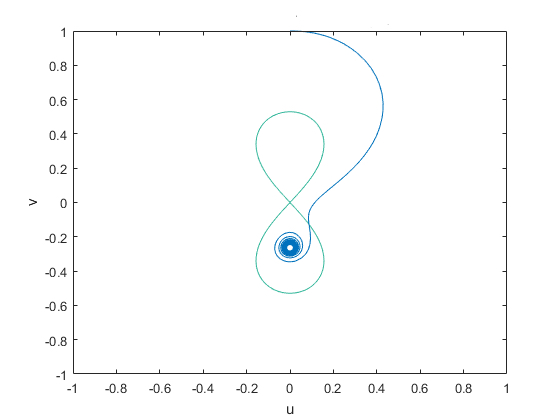
Figure 2: A solution entering the lower half-plane $\{v<0\}$.

To do so we relate solutions corresponding to such data to those of a limiting problem, inspired by [22].

2.2 Asymptotic expansion

In this section we provide, after a suitable scaling, a precise asymptotic expansion that will allow us to control the behavior of the solution in term of the initial datum.

Put $\varepsilon=\lambda^{-1}$ and consider the following rescaling

$$\left\{\begin{aligned} U_{\varepsilon}(r)&=\varepsilon u_{\lambda}(\varepsilon^{2}r)\\ V_{\varepsilon}(r)&=\varepsilon v_{\lambda}(\varepsilon^{2}r)\end{aligned}\right.$$ (38)

Using (17) we find the system for $(U_{\varepsilon},V_{\varepsilon})$:

$$\left\{\begin{aligned} \dot{U}_{\varepsilon}+\frac{U_{\varepsilon}}{r}&=(U^{2}_{\varepsilon}+V^{2}_{\varepsilon})V_{\varepsilon}-\varepsilon^{2}(m-\omega)V_{\varepsilon}\\ \dot{V}_{\varepsilon}&=-(U^{2}_{\varepsilon}+V^{2}_{\varepsilon})U_{\varepsilon}-\varepsilon^{2}(m+\omega)U_{\varepsilon}\end{aligned}\right.$$ (39)

together with the initial conditions $U_{\varepsilon}(0)=0$, $V_{\varepsilon}(0)=1$.

The limiting problem as $\varepsilon\rightarrow 0$ (and thus $\lambda\rightarrow+\infty$) is

$$\left\{\begin{aligned} \dot{U}_{0}+\frac{U_{0}}{r}&=(U^{2}_{0}+V_{0}^{2})V_{0}\\ \dot{V}_{0}&=-(U^{2}_{0}+V^{2}_{0})U_{0}\end{aligned}\right.$$ (40)

with $U_{0}(0)=0$, $V_{0}(0)=1$.

As in [23] we consider the family of spinors given by

$$\varphi(y)=f(y)(1-y)\cdot\varphi_{0}\qquad y\in\mathbb{R}^{2}$$ (41)

where $\varphi_{0}\in\mathbb{C}^{2}$, $f(y)=\frac{2}{1+|y|^{2}}$ and the dot represents the Clifford product.

It can be easily checked that they are $\mathring{H}^{\frac{1}{2}}(\mathbb{R}^{2},\mathbb{C}^{2})$-solutions to the following Dirac equation

$$\mathcal{D}\varphi=|\varphi|^{2}\varphi$$ (42)

Remark 12.

The spin structure of euclidean spaces is quite explicit and the spinors given in (41) can be rewritten in matrix notation, as

$$\varphi(y)=f(y)(\mathds{1}_{2}+iy_{1}\sigma_{1}+iy_{2}\sigma_{2})\cdot\varphi_{0}\qquad y\in\mathbb{R}^{2}$$

$\mathds{1}_{2}$ and $\sigma_{i}$ being the identity and the Pauli matrices, respectively.

See [24] for more details.

A straightforward (but tedious) computation shows that the spinors defined in (41) are of the form of the ansatz (16), thus being solutions to the system (40). Exploiting the conformal invariance of (42) (see [13]) one can easily see that the solution matching the above initial conditions is

$$\left(U_{0}(r)=\frac{2r}{4+r^{2}},V_{0}(r)=\frac{4}{4+r^{2}}\right)$$ (43)

Lemma 13.

We have

$$(U_{\varepsilon},V_{\varepsilon})\xrightarrow{\varepsilon\rightarrow 0}(U_{0},V_{0})$$

uniformly on $[0,T]$, for all $T>0$, where $(U_{0},V_{0})$ is the solutions to the limiting problem (40).

Proof.

Fix $T>0$ and let $r\in[0,T]$.

Remark that the system (39) is equivalent to

$$\left\{\begin{aligned} U_{\varepsilon}(r)&=\frac{1}{r}\int^{r}_{0}sV_{\varepsilon}(s)[U_{\varepsilon}^{2}(s)+V_{\varepsilon}^{2}(s)-\varepsilon^{2}(m-\omega)]ds\\ V_{\varepsilon}(r)&=1-\int^{r}_{0}U_{\varepsilon}(s)[(U^{2}_{\varepsilon}(s)+V^{2}_{\varepsilon}(s))+\varepsilon^{2}(m+\omega)]ds\end{aligned}\right.$$ (44)

Similarly, we can rewrite (40) as

$$\left\{\begin{aligned} U_{0}(r)&=\frac{1}{r}\int^{r}_{0}sV_{0}(s)(U_{0}^{2}(s)+V_{\varepsilon}^{2}(s))ds\\ V_{0}(r)&=1-\int^{r}_{0}U_{0}(s)(U^{2}_{0}(s)+V^{2}_{0}(s))ds\end{aligned}\right.$$ (45)

Arguing as for (17), for each fixed $\varepsilon>0$ we associate a hamiltonian to the system (39)

$$\widetilde{H}_{\varepsilon}(U,V):=\frac{(U^{2}+V^{2})^{2}}{4}+\varepsilon^{2}\frac{m}{2}(U^{2}-V^{2})+\varepsilon^{2}\frac{\omega}{2}(U^{2}+V^{2})$$

It’s easy to see that $\widetilde{H}_{\varepsilon}$ is decreasing along the flow, so that

$$\widetilde{H}_{\varepsilon}(U_{\varepsilon}(r),V_{\varepsilon}(r))\leqslant\widetilde{H}_{\varepsilon}(0,1)\leqslant 1\qquad\forall r\geqslant 0.$$

The coercivity of $H_{\varepsilon}$ then implies that

$$|U_{\varepsilon}(r)|+|V_{\varepsilon}(r)|\leqslant C\qquad\forall r\geqslant 0$$ (46)

for some $C>0$ independent of $\varepsilon$.

By (44,45) and since $r\in[0,T]$ we get

$$\begin{split}|U_{\varepsilon}(r)-U_{0}(r)|+&|V_{\varepsilon}(r)-V_{0}(r)|\leqslant\int^{r}_{0}\left|V_{\varepsilon}(V^{2}_{\varepsilon}+U^{2}_{\varepsilon})-V_{0}(V^{2}_{0}+U^{2}_{0})\right|ds\\ &+\int^{r}_{0}\left|U_{\varepsilon}(V^{2}_{\varepsilon}+U^{2}_{\varepsilon})-U_{0}(V^{2}_{0}+U^{2}_{0})\right|ds+2\varepsilon^{2}mT\end{split}$$ (47)

It’s not hard to see that the first two integrands in the r.h.s of the above inequality are locally Lipschitz. Then by (46) we have

$$|U_{\varepsilon}(r)-U_{0}(r)|+|V_{\varepsilon}(r)-V_{0}(r)|\lesssim\int^{r}_{0}\left(|U_{\varepsilon}-U_{0}|+|V_{\varepsilon}-V_{0}|\right)ds+2\varepsilon^{2}mT$$ (48)

Since $r\in[0,T]$, the Gronwall lemma gives

$$|U_{\varepsilon}(r)-U_{0}(r)|+|V_{\varepsilon}(r)-V_{0}(r)|\lesssim\varepsilon^{2}$$ (49)

thus proving the claim. ∎

The above results is not enough to conclude that $V_{\varepsilon}$ changes sign, since $V_{0}>0$ for all $r\geqslant 0$.

We obtain a more refined analysis of the behavior of the solution thanks to a continuity argument.

We consider the solution $(U_{\varepsilon},V_{\varepsilon})$ as a perturbation of $(U_{0},V_{0})$, as follows:

$$\left\{\begin{aligned} U_{\varepsilon}(r)&=U_{0}(r)+\varepsilon^{2}h_{1}(r)+\varepsilon^{4}h_{2}(r,\varepsilon)\\ V_{\varepsilon}(r)&=V_{0}(r)+\varepsilon^{2}k_{1}(r)+\varepsilon^{4}k_{2}(r,\varepsilon)\end{aligned}\right.$$ (50)

and substituting into (39) we get the following linear system for $\varepsilon^{2}$-order terms

$$\left\{\begin{aligned} \dot{h}_{1}+\frac{h_{1}}{r}&=-(m-\omega)V_{0}+2U_{0}V_{0}h_{1}+(U^{2}_{0}+3V^{2}_{0})k_{1}\\ \dot{k}_{1}&=-(m+\omega)U_{0}-2U_{0}V_{0}k_{1}-(3U^{2}_{0}+V^{2}_{0})h_{1}\end{aligned}\right.$$ (51)

and we impose the initial conditions

$$h_{1}(0)=0\qquad,\quad k_{1}(0)=0$$ (52)

Rewriting (51) in integral form, as in (22), we have:

$$\left\{\begin{aligned} |{h}_{1}(r)|&\leqslant\int^{r}_{0}(m-\omega)V_{0}ds+\int^{r}_{0}\left[2U_{0}V_{0}|h_{1}|+(U^{2}_{0}+3V^{2}_{0})|k_{1}|\right]ds\\ |{k}_{1}(r)|&\leqslant\int^{r}_{0}(m+\omega)U_{0}ds+\int^{r}_{0}\left[2U_{0}V_{0}|k_{1}|+(3U^{2}_{0}+V^{2}_{0})|h_{1}|\right]ds\end{aligned}\right.$$ (53)

Remark that

$$U_{0}V_{0}(r)+V^{2}_{0}(r)\leqslant U^{2}_{0}(r)\leqslant V_{0}\quad,\quad\forall r>2$$

and that

$$V_{0}\in L^{1}(\mathbb{R}^{+}).$$

Moreover, there holds

$$U_{0}(r)=\frac{2r}{4+r^{2}}\sim\frac{2}{r}\qquad\mbox{as}\quad r\longrightarrow+\infty.$$ (54)

Then summing up both sides of (53) we get:

$$|h_{1}(r)|+|k_{1}(r)|\lesssim\int^{r}_{0}U_{0}ds+\int^{r}_{0}\left(|h_{1}|+|k_{1}|\right)V_{0}ds$$ (55)

The Gronwall inequality thus gives:

$$|h_{1}(r)|+|k_{1}(r)|\lesssim\left(\int^{r}_{0}U_{0}ds\right)\exp\left(C\int^{r}_{0}V_{0}ds\right)\lesssim\int^{r}_{0}U_{0}ds$$ (56)

where $C>0$ is a constant.

By (54) we can thus conclude that

$$|h_{1}(r)|+|k_{1}(r)|\lesssim\ln(r)\qquad\mbox{as}\quad r\longrightarrow+\infty$$ (57)

The above estimates imply that

$$2U_{0}V_{0}k_{1},(3U^{2}_{0}+V^{2}_{0})h_{1}\in L^{1}(\mathbb{R}^{+})$$

and then integrating the second equation in (51) we get

$$h_{1}(r)\sim-\ln(r)\qquad\mbox{as}\quad r\longrightarrow+\infty$$ (58)

We now have to deal with remainder terms in (50).

In particular, we want to analyze the behavior of those terms on the time interval $\left(0,\frac{1}{\varepsilon}\right)$, thanks to a continuity argument based on the Gronwall inequality.

Let

$$\overline{r}_{\varepsilon}:=\sup\left\{r\in\left[0,\varepsilon^{-1}\right):|h_{2}(r,\varepsilon)|+|k_{2}(r,\varepsilon)|<\varepsilon^{-\frac{3}{2}}\right\}$$ (59)

Since $h_{2}(0,\varepsilon)=k_{2}(0,\varepsilon)=0$, by continuity it’s evident that

$$\overline{r}_{\varepsilon}>0$$

As shown in the Appendix using the equations for $h_{2}$ and $k_{2}$ one gets the following estimates:

$$|h_{2}(r,\varepsilon)|+|k_{2}(r,\varepsilon)|\lesssim\frac{1}{\varepsilon}\ln\left(\frac{1}{\varepsilon}\right)+\int^{r}_{0}\left(V_{0}(s)+\varepsilon^{2}\right)\left(|h_{2}(s,\varepsilon)|+|k_{2}(s,\varepsilon)|\right)ds$$ (60)

for $0<r<\overline{r}_{\varepsilon}\leqslant\frac{1}{\varepsilon}$.

The Gronwall estimates then gives:

$$|h_{2}(r,\varepsilon)|+|k_{2}(r,\varepsilon)|\lesssim\frac{1}{\varepsilon}\ln\left(\frac{1}{\varepsilon}\right)\exp\left(C\int^{r}_{0}\left(\varepsilon^{2}+V_{0}(s)\right)ds\right)$$ (61)

for some $C>0$.

Since $r<\frac{1}{\varepsilon}$ and $V_{0}\in L^{1}(\mathbb{R}^{+})$ we eventually have:

$$|h_{2}(r,\varepsilon)|+|k_{2}(r,\varepsilon)|\lesssim\frac{1}{\varepsilon}\ln\left(\frac{1}{\varepsilon}\right)$$ (62)

Now, if we suppose that

$$\overline{r}_{\varepsilon}<\frac{1}{\varepsilon}$$

by (62) and by continuity there exists $\delta>0$ such that

$$\frac{1}{\varepsilon}\ln\left(\frac{1}{\varepsilon}\right)\lesssim|h_{2}(r,\varepsilon)|+|k_{2}(r,\varepsilon)|\leqslant\varepsilon^{-\frac{3}{2}}$$

for all $r\in[\overline{r}_{\varepsilon},\overline{r}_{\varepsilon}+\delta)$, thus contradicting the definition in (59).

Then there holds:

$$|h_{2}(r,\varepsilon)|+|k_{2}(r,\varepsilon)|<\varepsilon^{-\frac{3}{2}},\qquad\forall r\in\left(0,\frac{1}{\varepsilon}\right)$$ (63)

Recall that the second equation in (50) reads as

$$V_{\varepsilon}(r)=V_{0}(r)+\varepsilon^{2}k_{1}(r)+\varepsilon^{4}k_{2}(r,\varepsilon)$$

By (62) and (43) we see that

$$V_{0}=O(\varepsilon^{2})\quad,\quad k_{2}=o(\varepsilon^{2})\qquad\mbox{as}\quad r\rightarrow\left(\frac{1}{\varepsilon}\right)^{-}$$

Then by (58) we get

$$V_{\varepsilon}(r)\sim-\varepsilon^{2}\ln{\frac{1}{\varepsilon}}\qquad\mbox{as}\quad r\rightarrow\left(\frac{1}{\varepsilon}\right)^{-}$$ (64)

Thus we have

$$V_{\varepsilon}(R_{\varepsilon})=0\qquad\mbox{for some}\quad R_{\varepsilon}\in\left(0,\frac{1}{\varepsilon}\right)$$ (65)

In view of the scaling (38), we conclude that for large initial data $\lambda>0$, the corresponding solution $(u_{\lambda},v_{\lambda})$ of (17) has at least one node.

This proves the following (recall the definition (11))

Lemma 14.

The set $A_{0}$ is bounded.

Then by (Lemma 11) we have that $I_{0}\neq\emptyset$, that is the system (17) admits a solution without nodes, tending to $(0,0)$ as $r\rightarrow+\infty$, which correspond to a localised solution of equation (4). The exponential decay follows by (Lemma 9). This proves (Theorem 1).

Appendix

In this section we prove the estimates (60) for remainder terms in (50).

For the sake of brevity we only deal with $k_{2}$. The estimate for $h_{2}$ follows along the same lines with obvious modifications.

Inserting the ansatz (50) into the system (39), using equations (43) and (51) and imposing the initial condition we get the following equation

$$\left\{\begin{aligned} \frac{d}{dr}k_{2}(r,\varepsilon)&=K_{0}(r)+\varepsilon^{2}K_{2}(r)+\varepsilon^{4}K_{4}(r)+\varepsilon^{6}K_{6}(r)+\varepsilon^{8}K_{8}(r)\\ k_{2}(0,\varepsilon)&=0\end{aligned}\right.$$ (66)

for all $\varepsilon>0$. Note that the $K^{i}$s do not depend on $\varepsilon$.

The terms in the r.h.s. are given by

$$\left\{\begin{aligned} K_{0}&=-\left(2U^{2}_{0}+V^{2}_{0}+2U_{0}V_{0}\right)h_{2}-U_{0}\left(3h^{2}_{1}+k^{2}_{1}\right)-2V_{0}h_{1}k_{1}-(m+\omega)h_{1}\\ K_{2}&=-U_{0}\left(4h_{1}h_{2}+2k_{1}k_{2}\right)-(h^{3}_{1}+h_{1}k^{2}_{1})-2V_{0}(h_{1}k_{2}+k_{1}h_{2})-(m+\omega)h_{2}\\ K_{4}&=-\left(U_{0}(2h^{2}_{2}+k^{2}_{2})+2V_{0}h_{2}k_{2}\right)-(2h_{1}k_{1}k_{2}+2h^{2}_{1}h_{2}+k^{2}_{1}h_{2})\\ K_{6}&=-h_{1}h^{2}_{2}-k_{1}k^{2}_{2}-h_{1}h^{2}_{2}-k_{1}k_{2}h_{2}\\ K_{8}&=-h^{3}_{2}-h_{2}k^{2}_{2}\end{aligned}\right.$$ (67)

Our aim is to estimate $|k_{2}(r,\varepsilon)|$ for $0<r<\overline{r}$ (see (59)) and $0<\varepsilon\ll 1$.

This is achieved integrating (66) and estimating the integral of the absolute value of each term in (67).

Remark that, by the definition of $(U_{0},V_{0})$, (43)

$$2U^{2}_{0}+V^{2}_{0}+2U_{0}V_{0}\leqslant V_{0}\in L^{1}(\mathbb{R}^{+})$$ (68)

Moreover, (57) and (54) imply that $U_{0}\left(3h^{2}_{1}+k^{2}_{1}\right)\notin L^{1}(\mathbb{R}^{+})$ and then

$$\int^{r}_{0}U_{0}\left|3h^{2}_{1}+k^{2}_{1}\right|ds\lesssim\int^{\frac{1}{\varepsilon}}_{1}\frac{\ln(s)}{s}ds\lesssim\varepsilon^{-\frac{1}{4}}$$ (69)

By the above remarks and (57), we have

$$V_{0}h_{1}k_{1}\in L^{1}(\mathbb{R}^{+})$$ (70)

and

$$\int^{r}_{0}|h_{1}|ds=O(r\ln(r)),\qquad\mbox{as}\quad r\rightarrow+\infty$$ (71)

Collecting the above esimates we get

$$\int^{r}_{0}|K_{0}|ds\lesssim\int^{r}_{0}V_{0}|h_{2}|ds+\varepsilon^{-1}|\ln(\varepsilon)|$$ (72)

The second term is estimated as follows.

Recall that

$$|h_{2}(r)|+|k_{2}(r)|\leqslant\varepsilon^{-\frac{3}{2}}$$ (73)

for $0<r\leqslant\overline{r}$. Then by (68) we have

$$\int^{r}_{0}U_{0}\left|4h_{1}h_{2}+2k_{1}k_{2}\right|ds\lesssim\varepsilon^{-\frac{3}{2}}\int^{\frac{1}{\varepsilon}}_{1}\frac{\ln(s)}{s}ds\lesssim\varepsilon^{-\frac{7}{4}}$$ (74)

Using again (57), it’s not hard to see that

$$\int^{r}_{0}|h^{3}_{1}+h_{1}k^{2}_{1}|ds\lesssim\varepsilon^{-\frac{5}{4}}$$ (75)

Since

$$V_{0}h_{1},V_{0}k_{1}\in L^{1}(\mathbb{R}^{+})$$

by (73) we have

$$\int^{r}_{0}V_{0}\left(|h_{1}k_{2}|+|k_{1}h_{2}|\right)ds\lesssim\varepsilon^{-\frac{3}{2}}$$ (76)

We then conclude that

$$\int^{r}_{0}|K_{2}|ds\lesssim\varepsilon^{-\frac{7}{4}}+\int^{r}_{0}|h_{2}|ds$$ (77)

Let’s turn to the third term.

By (68) and (73) and since $U_{0}(r)=\frac{2r}{4+r^{2}}$, we get

$$\int^{r}_{0}|U_{0}(2h^{2}_{2}+k^{2}_{2})+2V_{0}h_{2}k_{2}|ds\lesssim\varepsilon^{-3}\int^{\frac{1}{\varepsilon}}_{1}U_{0}ds\lesssim\varepsilon^{-3}|\ln(\varepsilon)|$$ (78)

Using (57) and (73) we can estimate

$$\int^{\overline{r}}_{0}|K_{4}|ds\lesssim\varepsilon^{-3}|\ln(\varepsilon)|+\varepsilon^{-\frac{5}{4}}\lesssim\varepsilon^{-3}|\ln(\varepsilon)|$$ (79)

All the terms appearing in $K_{6}$ have the same behavior, so that by (57),(73) and above estimates it’s easy to see that

$$\int^{r}_{0}|K_{6}|ds\lesssim\varepsilon^{-4}|\ln(\varepsilon)|$$ (80)

Lastly, by (73) we can estimate

$$\int^{r}_{0}|K_{8}|ds\lesssim\varepsilon^{-\frac{11}{2}}$$ (81)

Combining (72,77,79,80,81), integrating (67) gives

$$|k_{2}(r,\varepsilon)|\lesssim\varepsilon^{-1}|\ln(\varepsilon)|+\int^{r}_{0}(V_{0}(s)+\varepsilon^{2})|h_{2}(s,\varepsilon)|ds$$ (82)

Analogous estimates can be worked out for $h_{2}$, obtaining

$$|h_{2}(r,\varepsilon)|\lesssim\varepsilon^{-1}|\ln(\varepsilon)|+\int^{r}_{0}(V_{0}(s)+\varepsilon^{2})|k_{2}(s,\varepsilon)|ds$$ (83)

and the claimed inequality (60) follows by summing up the last two estimates.

References

References

[1]
M. J. Esteban, M. Lewin, E. Séré, Variational methods in relativistic
quantum mechanics, Bull. Amer. Math. Soc. (N.S.) 45 (4) (2008) 535–593.
doi:10.1090/S0273-0979-08-01212-3.
[2]
A. Castro Neto, F. Guinea, N. Peres, K. Novoselov, A. Geim, The electronic
properties of graphene, Comptes Rendus Physique 14 (9-10) (2013) 760–778.
[3]
A. B. T.O. Wehling, A.M. Black-Schaffer, Dirac materials, Adv.Phys.. 63 (1)
(2014) 1–76.
[5]
J. Cayssol, Introduction to dirac materials and topological insulators, Rev.
Mod. Phys. 109 (81).
[6]
C. L. Fefferman, M. I. Weinstein, Honeycomb lattice potentials and dirac
points, J. Amer. Math. Soc. 25 (4) (2012) 1169–1220.
doi:10.1090/S0894-0347-2012-00745-0.
[7]
C. L. Fefferman, J. P. Lee-Thorp, M. I. Weinstein, Topologically protected
states in one-dimensional continuous systems and Dirac points, Proc. Natl.
Acad. Sci. USA 111 (24) (2014) 8759–8763.
doi:10.1073/pnas.1407391111.
[9]
L. Pitaevskii, S. Stringari, Bose-Einstein condensation, Vol. 116 of
International Series of Monographs on Physics, The Clarendon Press, Oxford
University Press, Oxford, 2003.
[10]
J. Moloney, A. Newell, Nonlinear optics, Westview Press. Advanced Book Program,
Boulder, CO, 2004.
[12]
M. Struwe, Variational methods, 4th Edition, Vol. 34 of Ergebnisse der
Mathematik und ihrer Grenzgebiete. 3. Folge. A Series of Modern Surveys in
Mathematics [Results in Mathematics and Related Areas. 3rd Series. A Series
of Modern Surveys in Mathematics], Springer-Verlag, Berlin, 2008,
applications to nonlinear partial differential equations and Hamiltonian
systems.
[13]
T. Isobe, Nonlinear Dirac equations with critical nonlinearities on compact
Spin manifolds, J. Funct. Anal. 260 (1) (2011) 253–307.
doi:10.1016/j.jfa.2010.09.008.
[14]
T. Cazenave, L. Vázquez, Existence of localized solutions for a classical
nonlinear Dirac field, Comm. Math. Phys. 105 (1) (1986) 35–47.
[16]
M. J. Esteban, S. Rota Nodari, Symmetric ground states for a stationary
relativistic mean-field model for nucleons in the non-relativistic limit,
Rev. Math. Phys. 24 (10) (2012) 1250025, 30.
doi:10.1142/S0129055X12500250.
[17]
L. c. Le Treust, S. Rota Nodari, Symmetric excited states for a mean-field
model for a nucleon, J. Differential Equations 255 (10) (2013) 3536–3563.
doi:10.1016/j.jde.2013.07.041.
[19]
Y. Ding, J. Wei, Stationary states of nonlinear Dirac equations with general
potentials, Rev. Math. Phys. 20 (8) (2008) 1007–1032.
doi:10.1142/S0129055X0800350X.
[20]
Y. Ding, B. Ruf, Existence and concentration of semiclassical solutions for
Dirac equations with critical nonlinearities, SIAM J. Math. Anal. 44 (6)
(2012) 3755–3785.
doi:10.1137/110850670.
[21]
J. Cuevas-Maraver, P. G. Kevrekidis, A. Saxena, A. Comech, R. Lan, Stability of
solitary waves and vortices in a 2D nonlinear Dirac model, Phys. Rev.
Lett. 116 (21) (2016) 214101, 6.
[22]
K. McLeod, W. C. Troy, F. B. Weissler, Radial solutions of
with prescribed numbers of zeros, J. Differential Equations 83 (2) (1990)
368–378.
doi:10.1016/0022-0396(90)90063-U.
[23]
B. Ammann, J.-F. Grosjean, E. Humbert, B. Morel, A spinorial analogue of
Aubin’s inequality, Math. Z. 260 (1) (2008) 127–151.
doi:10.1007/s00209-007-0266-5.
[24]
J. Jost, Riemannian geometry and geometric analysis, sixth Edition,
Universitext, Springer, Heidelberg, 2011.
doi:10.1007/978-3-642-21298-7.