Numerical assessment of two-level domain decomposition preconditioners for incompressible Stokes and elasticity equations

Abstract

Solving the linear elasticity and Stokes equations by an optimal domain decomposition method derived algebraically involves the use of non standard interface conditions. The one-level domain decomposition preconditioners are based on the solution of local problems. This has the undesired consequence that the results are not scalable, it means that the number of iterations needed to reach convergence increases with the number of subdomains. This is the reason why in this work we introduce, and test numerically, two-level preconditioners. Such preconditioners use a coarse space in their construction. We consider the nearly incompressible elasticity problems and Stokes equations, and discretise them by using two finite element methods, namely, the hybrid discontinuous Galerkin and Taylor-Hood discretisations.

Key words. Stokes problem, nearly incompressible elasticity, Taylor-Hood, hybrid discontinuous Galerkin methods, domain decomposition, coarse space, optimized restricted additive Schwarz methods

1 Introduction

In [BBD⁺16] the one-level domain decomposition methods for Stokes equations were introduced in conjunction with the non standard interface conditions. Although it can be observed there the lack of scalability with respect to the number of subdomains. It means that by splitting the problem in a larger number of subdomains leads to the increase of size of the plateau region in the convergence of an iterative method (see Figure 1) when using the one-level domain decomposition methods. This is caused by the lack of global information, as subdomains can only communicate with their neighbours. Hence, when the number of subdomains increases in one direction, the length of the plateau also increases. Even in cases when the local problems are of the same size, the iteration count grows with the increase of the number of subdomain. This can be also observed in all experiments in this manuscript in case of one-level methods.

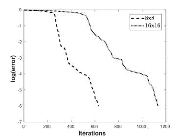
(a) Taylor-Hood

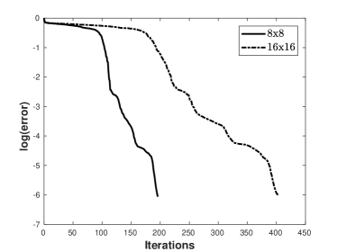
(b) hdG

Figure 1: Increase of the size of the plateau region for increasing number of subdomains.

The remedy for this is the use of a second level in the preconditioner or a coarse space correction that adds the necessary global information. Two-level algorithms have been analysed for several classes of problems in [TW05]. The key point of these kind of methods is to choose the appropriate coarse space. The classical coarse space introduced by Nicolaides in [Nic87] is defined by vectors that support is in each subdomain. Hence the coarse space has the size equal to a number of subdomains. A coarse space construction, named spectral coarse space, was motivated by the complexity of the problems that classical coarse space performance was not satisfying. This construction allows to enrich a bigger size of the coarse space, but can be also reduced to the classical one. This idea was introduced for the first time in [BHMV99] in the case of multigrid methods. It relies on solving local generalised eigenvalue problems allowing to choose suitable vectors for the coarse space.

For overlapping domain decomposition preconditioners, a similar idea was introduced in the case of Darcy equations in [GE10a, GE10b]. The authors of [NXD10] consider also the heterogeneous Darcy equation and presented a different generalised eigenvalue problem based on local Dirichlet-to-Neumann maps. The method has been analysed in [DNSS12] and proved to be very robust in the case of small overlaps. The same idea was extended numerically to the heterogeneous Helmholtz problem in [CDKN14]. The authors of [LNS15] apply the coarse space associated with low-frequency eigenfunctions of the subdomain Dirichlet-to-Neumann maps for the generalisation of the optimised Schwarz methods, named 2-Lagrange multiplier methods.

The first attempt to extend this spectral approach to general symmetric positive definite problems was made in [EGLW12] as an extension of [GE10a, GE10b]. Since some of the assumptions of the previous framework are hard to fulfil, authors of [SDH⁺14] proposed slightly different approach for symmetric positive definite problems. Their idea of constructing partition of unity operator associated with degrees of freedom allows to work with various finite element spaces. An overview of different kinds of two-level methods can be found in [DJN15, Chapters 5 and 7].

Despite the fact that all these approaches provide satisfying results, there is no universal treatment to build efficient coarse spaces in the case of non definite problems such as Stokes equations. The spectral coarse spaces that we use in this work are inspired by those proposed in [HJN15]. The authors introduced and tested numerically symmetrised two-level preconditioners for overlapping algorithms which use Robin interface conditions between the subdomains (see (5.27) for details). They have applied these preconditioners to solve saddle point problems such as nearly incompressible elasticity and Stokes discretised by Taylor-Hood finite elements. In our case, we use non standard interface conditions. Therefore the use of spectral coarse spaces could lead to an important gain.

In this work, we test this improvement in case of nearly incompressible elasticity and Stokes equations that are discussed in Section 2. As the discretisations we use the Taylor-Hood [GR86, Chapter II, Section 4.2] and hybrid discontinuous Galerkin method [CGL09, CG09] presented in Section 3. In Section 4 we introduce the two-level domain decomposition preconditioners. Sections 5 and 6 present the two and three dimensional numerical experiments, respectively. Finally, a summary is outlined in Section 7.

2 The differential equations

Let $\Omega$ be an open polygon in $\mathbb{R}^{2}$ or an open Lipschitz polyhedron in $\mathbb{R}^{3}$, with Lipschitz boundary $\Gamma:=\partial\Omega$. We use $d=2,3$ to denote the dimension of the space. We use bold for tensor or vector variables. In addition we denote normal and tangential components as follows ${u_{n}}:=\boldsymbol{u}\cdot\boldsymbol{n}$, and $u_{t}:=\boldsymbol{u}-u_{n}\boldsymbol{n}$, where $\boldsymbol{n}$ is the outward unit normal vector to the boundary $\Gamma$ .

For $D\subset\Omega$, we use the standard $L^{2}(D)$ space and $C^{0}(\bar{D})$ denotes the set of all continuous functions on the closure of a set $D$. Let us define following Sobolev spaces

$$H^{m}(D) :=\left\{v\in L^{2}(D):\ \forall\ |\boldsymbol{\alpha}|\leq m\ \partial^{\boldsymbol{\alpha}}{v}\in L^{2}(D)\right\}\mbox{ for }m\in\mathbb{N},$$

$$H^{\frac{1}{2}}(\partial D) :=\left\{\tilde{v}\in L^{2}(\partial D):\ \exists v\in H^{1}(D)\quad\tilde{v}=\mbox{tr}(v)\right\},$$

$$H\left(div,D\right) :=\left\{\boldsymbol{v}\in[L^{2}(D)]^{d}:\ \nabla\cdot\boldsymbol{v}\in L^{2}(D)\right\},$$

where, for $\boldsymbol{\alpha}=(\alpha_{1},...,\alpha_{d})\in\mathbb{N}^{d}$ and $|\boldsymbol{\alpha}|=\sum_{i=1}^{d}\alpha_{i}$ we denote $\partial^{\boldsymbol{\alpha}}=\frac{\partial^{|\boldsymbol{\alpha}|}}{\partial x_{1}^{\alpha_{1}}...\partial x_{d}^{\alpha_{d}}}$, and $\mbox{tr}:H^{1}(\Omega)\rightarrow H^{\frac{1}{2}}(\partial\Omega)$ is the trace operator. In addition, we use the following notation of the space including boundary and average conditions

$$L^{2}_{0}(D) :=\left\{v\in L^{2}(D):\ \int_{D}v\ d\boldsymbol{x}=0\right\},$$

$$H^{1}_{\tilde{\Gamma}}(D) :=\left\{v\in H^{1}(D):\ v=0\mbox{ on }\tilde{\Gamma}\right\},$$

where $\tilde{\Gamma}\subset\partial D$. If $\tilde{\Gamma}=\partial D$, then $H^{1}_{\tilde{\Gamma}}(D)$ is denoted $H^{1}_{0}(D)$.

Now we present the two differential problems considered in this work.

2.1 Stokes equation

Let us start with $d$-dimensional, $d=2,3$, Stokes problem

(2.1) $$\left\{\begin{array}[]{rclclr}-\nu\Delta\boldsymbol{u}&\ +&\nabla p&=&\boldsymbol{f}&\mbox{in }\Omega\\ &&\nabla\cdot\boldsymbol{u}&=&0&\mbox{in }\Omega\end{array}\right.,$$

where $\boldsymbol{u}:\bar{\Omega}\rightarrow\mathbb{R}^{d}$ is the velocity field, $p:\bar{\Omega}\rightarrow\mathbb{R}$ the pressure, $\nu>0$ the viscosity which is considered to be constant and $\boldsymbol{f}\in[L^{2}(\Omega)]^{d}$ is a given function. We define the stress tensor $\boldsymbol{\sigma}:=\nu\nabla\boldsymbol{u}-p\boldsymbol{I}$ and the flux as $\boldsymbol{\sigma_{n}}:=\boldsymbol{\sigma}\ \boldsymbol{n}$. For $\boldsymbol{u_{D}}\in[H^{\frac{1}{2}}(\Gamma)]^{d}$ and ${g}\in L^{2}(\Gamma)$ we consider three types of boundary conditions:

• Dirichlet (non-slip)

  (2.2) $$\boldsymbol{u}=\boldsymbol{u_{D}}\mbox{ on }\Gamma;$$

• tangential-velocity and normal-flux (TVNF)

  (2.3) $$\left\{\begin{array}[]{rcll}u_{t}&=&0&\mbox{ on }\Gamma\\ {\sigma_{nn}}&=&{g}&\mbox{ on }\Gamma\end{array}\right.;$$

• normal-velocity and tangential-flux (NVTF)

  (2.4) $$\left\{\begin{array}[]{rcll}{u_{n}}&=&0&\mbox{ on }\Gamma\\ {\sigma_{nt}}&=&{g}&\mbox{ on }\Gamma\end{array}\right..$$

The third type of boundary condition has already been considered for the Stokes problem in [AdDBM⁺14].

2.2 Nearly incompressible elasticity equation

From a mathematical point of view, the nearly incompressible elasticity problem is very similar to the Stokes equations. The difference is that instead of considering the gradient $\nabla\boldsymbol{v}$, the symmetric gradient $\boldsymbol{\varepsilon}(\boldsymbol{v}):=\frac{1}{2}\left(\nabla\boldsymbol{v}+\nabla^{T}\boldsymbol{v}\right)$ is used. We want to solve the following $d$-dimensional, $d=2,3$, problem

(2.5) $$\left\{\begin{array}[]{rclclr}-2\mu\nabla\cdot\boldsymbol{\varepsilon}(\boldsymbol{u})&+&\nabla p&=&\boldsymbol{f}&\mbox{in }\Omega\\ &-&\nabla\cdot\boldsymbol{u}&=&\frac{1}{\lambda}p&\mbox{in }\Omega\end{array}\right.$$

where $\boldsymbol{u}:\bar{\Omega}\rightarrow\mathbb{R}^{d}$ is the displacement field, $p:\Omega\rightarrow\mathbb{R}$ the pressure, $\boldsymbol{f}\in[L^{2}(\Omega)]^{d}$ is a given function, $\lambda$ and $\mu$ are the Lamé coefficients defined by

$$\lambda=\frac{E\nu}{(1+\nu)(1-2\nu)}, \mu=\frac{E}{2(1+\nu)},$$

where $E$ is the Young modulus and $\nu$ the Poisson ratio. We define the stress tensor as $\boldsymbol{\sigma}^{sym}:=2\mu\boldsymbol{\varepsilon}(\boldsymbol{u})-p\boldsymbol{I}$ and its normal component as $\boldsymbol{\sigma}^{sym}_{\boldsymbol{n}}:=\boldsymbol{\sigma}^{sym}\boldsymbol{n}$. For ${g}\in L^{2}(\Gamma)$ we consider three types of boundary conditions:

• mixed such that $\Gamma=\Gamma_{D}\cup\Gamma_{N}$ and $\Gamma_{D}\cap\Gamma_{N}=\emptyset$

  (2.6) $$\left\{\begin{array}[]{rcll}\boldsymbol{u}&=&0&\mbox{ on }\Gamma_{D}\\ \boldsymbol{\sigma_{n}^{sym}}&=&0&\mbox{ on }\Gamma_{N}\end{array}\right.;$$

• tangential-displacement and normal-normal-stress (TDNNS)

  (2.7) $$\left\{\begin{array}[]{rcll}u_{t}&=&0&\mbox{ on }\Gamma\\ {\sigma_{nn}^{sym}}&=&{g}&\mbox{ on }\Gamma\end{array}\right.;$$

• normal-displacement and tangential-normal-stress (NDTNS)

  (2.8) $$\left\{\begin{array}[]{rcll}{u_{n}}&=&0&\mbox{ on }\Gamma\\ {\sigma_{nt}^{sym}}&=&{g}&\mbox{ on }\Gamma\end{array}\right..$$

The second type of boundary condition has already been considered for linear elasticity equation in [PS11].

3 The numerical methods

Let $\left\{\mathcal{T}_{h}\right\}_{h>0}$ be a regular family of triangulations of $\bar{\Omega}$ made of simplices. For each triangulation $\mathcal{T}_{h}$, $\mathcal{E}_{h}$ denotes the set of its facets (edges for $d=2$, faces for $d=3$). In addition, for each element $K\in\mathcal{T}_{h}$, $h_{K}:=\mbox{diam}(K)$, and we denote $h:=\max_{K\in\mathcal{T}_{h}}h_{K}$. We define the following broken Sobolev spaces on the set of all edges in $\mathcal{E}_{h}$ (for $d=2$)

$$L^{2}(\mathcal{E}_{h}) :=\left\{v:\ v|_{E}\in L^{2}(E)\ \forall\ E\in\mathcal{E}_{h}\right\}.$$

Moreover, for $D\subset\Omega$, $\mathbb{P}_{k}(D)$ denotes the space of polynomials of total degree smaller than, or equal to, $k$ on the set $D$.

We now present the two discretisations to be used in the numerical experiments.

3.1 Taylor-Hood discretisation

We first consider the Taylor-Hood discretisation using the following approximation spaces

$$\boldsymbol{TH^{k}_{h}} :=\left\{\boldsymbol{v_{h}}\in[H^{1}(\Omega)]^{d}:\quad\boldsymbol{v_{h}}|_{K}\in[\mathbb{P}_{k}(K)]^{d}\quad\forall\ K\in\mathcal{T}_{h}\right\},$$

$$R^{k-1}_{h} :=\left\{q_{h}\in C^{0}(\bar{\Omega}):\quad q_{h}|_{K}\in\mathbb{P}_{k-1}(K)\quad\forall\ K\in\mathcal{T}_{h}\right\}$$

where $k\geq 2$ (see [GR86, Chapter II, Section 4.2]).

If (2.1) is supplied with the homogeneous boundary conditions (2.2), then the discrete problem reads:

Find $\left(\boldsymbol{u_{h}},p_{h}\right)\in\left(\left(\boldsymbol{TH^{k}_{h}}\cap[H_{0}^{1}(\Omega)]^{d}\right)\right)\times\left(R^{k-1}_{h}\cap L_{0}^{2}(\Omega)\right)$
s.t. for all $\left(\boldsymbol{v_{h}},q_{h}\right)\in\left(\left(\boldsymbol{TH^{k}_{h}}\cap[H_{0}^{1}(\Omega)]^{d}\right)\right)\times\left(R^{k-1}_{h}\cap L_{0}^{2}(\Omega)\right)$

(3.9) $$\left\{\begin{array}[]{rclcl}\displaystyle\int_{\Omega}\nu\nabla\boldsymbol{u_{h}}:\nabla\boldsymbol{v_{h}}\ d\boldsymbol{x}&-&\displaystyle\int_{\Omega}p_{h}\nabla\cdot\boldsymbol{v_{h}}\ d\boldsymbol{x}&=&\displaystyle\int_{\Omega}\boldsymbol{f}\boldsymbol{v_{h}}\ d\boldsymbol{x}\\ &-&\displaystyle\int_{\Omega}\nabla\cdot\boldsymbol{u_{h}}q_{h}\ d\boldsymbol{x}&=&0.\end{array}\right.$$

In case of TVNF boundary conditions (2.3), we define $\boldsymbol{V_{t}}:=\left\{\boldsymbol{v}\in[H^{1}(\Omega)]^{d}:\ v_{t}=0\mbox{ on }\Gamma\right\}$, and the discrete problem reads:

Find $\left(\boldsymbol{u_{h}},p_{h}\right)\in\left(\boldsymbol{TH^{k}_{h}}\cap\boldsymbol{V_{t}}\right)\times R^{k-1}_{h}$
s.t. for all $\left(\boldsymbol{v_{h}},q_{h}\right)\in\left(\boldsymbol{TH^{k}_{h}}\cap\boldsymbol{V_{t}}\right)\times R^{k-1}_{h}$

(3.10) $$\left\{\begin{array}[]{rclcl}\displaystyle\int_{\Omega}\nu\nabla\boldsymbol{u_{h}}:\nabla\boldsymbol{v_{h}}\ d\boldsymbol{x}&-&\displaystyle\int_{\Omega}p_{h}\nabla\cdot\boldsymbol{v_{h}}\ d\boldsymbol{x}&=&\displaystyle\int_{\Omega}\boldsymbol{f}\boldsymbol{v_{h}}\ d\boldsymbol{x}+\displaystyle\int_{\Gamma}g\left(\boldsymbol{v_{h}}\right)_{t}\ ds\\ &-&\displaystyle\int_{\Omega}\nabla\cdot\boldsymbol{u_{h}}q_{h}\ d\boldsymbol{x}&=&0.\end{array}\right.$$

If NVTF boundary conditions (2.4) are used, then we define the following space
$\boldsymbol{V_{n}}:=\left\{\boldsymbol{v}\in[H^{1}(\Omega)]^{d}:\ v_{n}=0\mbox{ on }\Gamma\right\}$, and the discrete problem reads:

Find $\left(\boldsymbol{u_{h}},p_{h}\right)\in\left(\boldsymbol{TH^{k}_{h}}\cap\boldsymbol{V_{n}}\right)\times\left(R^{k-1}_{h}\cap L_{0}^{2}(\Omega)\right)$
s.t. for all $\left(\boldsymbol{v_{h}},q_{h}\right)\in\left(\boldsymbol{TH^{k}_{h}}\cap\boldsymbol{V_{n}}\right)\times\left(R^{k-1}_{h}\cap L_{0}^{2}(\Omega)\right)$

(3.11) $$\left\{\begin{array}[]{rclcl}\displaystyle\int_{\Omega}\nu\nabla\boldsymbol{u_{h}}:\nabla\boldsymbol{v_{h}}\ d\boldsymbol{x}&-&\displaystyle\int_{\Omega}p_{h}\nabla\cdot\boldsymbol{v_{h}}\ d\boldsymbol{x}&=&\displaystyle\int_{\Omega}\boldsymbol{f}\boldsymbol{v_{h}}\ d\boldsymbol{x}+\displaystyle\int_{\Gamma}g\left(\boldsymbol{v_{h}}\right)_{n}\ ds\\ &-&\displaystyle\int_{\Omega}\nabla\cdot\boldsymbol{u_{h}}q_{h}\ d\boldsymbol{x}&=&0.\end{array}\right.$$

In similar way, if the problem (2.5) is supplied with the boundary conditions (2.6), then the discrete problem reads

Find $\left(\boldsymbol{u_{h}},p_{h}\right)\in\left(\boldsymbol{TH^{k}_{h}}\cap[H_{\Gamma_{D}}^{1}(\Omega)]^{d}\right)\times R^{k-1}_{h}$
s.t. for all $\left(\boldsymbol{v_{h}},q_{h}\right)\in\left(\boldsymbol{TH^{k}_{h}}\cap[H_{\Gamma_{D}}^{1}(\Omega)]^{d}\right)\times R^{k-1}_{h}$

(3.12) $$\left\{\begin{array}[]{rclcl}\displaystyle\int_{\Omega}2\mu\boldsymbol{\varepsilon}\left(\boldsymbol{u_{h}}\right):\boldsymbol{\varepsilon}\left(\boldsymbol{v_{h}}\right)\ d\boldsymbol{x}&-&\displaystyle\int_{\Omega}p_{h}\nabla\cdot\boldsymbol{v_{h}}\ d\boldsymbol{x}&=&\displaystyle\int_{\Omega}\boldsymbol{f}\boldsymbol{v_{h}}\ d\boldsymbol{x}\\ -\displaystyle\int_{\Omega}\nabla\cdot\boldsymbol{u_{h}}q_{h}\ d\boldsymbol{x}&-&\frac{1}{\lambda}\displaystyle\int_{\Omega}p_{h}q_{h}\ d\boldsymbol{x}&=&0.\end{array}\right.$$

The rest of the discrete problems associated with (2.5) that is supplied with TDNNS boundary conditions (2.7) or NDTNS boundary conditions (2.8) are similar to (3.10) or (3.11), respectively.

3.2 Hybrid discontinuous Galerkin discretisation

We restrict the discussion of this to two dimensional case $d=2$. This method has been presented and analysed in [BBD⁺16]. The velocity is approximated using the Brezzi-Douglas-Marini spaces (see [BBF13, Section 2.3.1]) of degree $k$ given by

$$\boldsymbol{BDM_{h}^{k}} :=\left\{\boldsymbol{v_{h}}\in H\left(div,\Omega\right):\ \boldsymbol{v_{h}}|_{K}\in\left[\mathbb{P}_{k}\left(K\right)\right]^{2}\ \forall\ {K\in\mathcal{T}_{h}}\right\},$$

$$\boldsymbol{BDM_{h,\tilde{\Gamma}}^{k}} :=\left\{\boldsymbol{v_{h}}\in H\left(div,\Omega\right):\ \boldsymbol{v_{h}}|_{K}\in\left[\mathbb{P}_{k}\left(K\right)\right]^{2}\ \forall\ {K\in\mathcal{T}_{h}}\land\ {\left(\boldsymbol{v_{h}}\right)_{n}}=0\mbox{ on }\tilde{\Gamma}\right\},$$

where $\tilde{\Gamma}\subset\partial\Omega$. If $\tilde{\Gamma}=\partial\Omega$, then $\boldsymbol{BDM_{h,\tilde{\Gamma}}^{k}}$ is denoted $\boldsymbol{BDM_{h,0}^{k}}$.

The pressure is approximated in the space

$$Q_{h}^{k-1} :=\left\{q_{h}\in L^{2}\left(\Omega\right):\ q_{h}|_{K}\in\mathbb{P}_{k-1}\left(K\right)\ \forall\ {K\in\mathcal{T}_{h}}\right\}.$$

Finally, a Lagrange multiplier, aimed at approximating the tangential component of the velocity is introduced. The space swhere this multipliers is sought are given by

$$M_{h}^{k-1} :=\left\{\tilde{v}_{h}\in L^{2}\left(\mathcal{E}_{h}\right):\ \tilde{v}_{h}|_{E}\in\mathbb{P}_{k-1}\left(E\right)\ \forall\ {E\in\mathcal{E}_{h}}\right\},$$

$$M_{h,\tilde{\Gamma}}^{k-1} :=\left\{\tilde{v}_{h}\in M_{h}^{k-1}:\tilde{v}_{h}=0\mbox{ on }\tilde{\Gamma}\right\},$$

where $\tilde{\Gamma}\subset\partial\Omega$. If $\tilde{\Gamma}=\partial\Omega$, then $M_{h,\tilde{\Gamma}}^{k-1}$ is denoted $M_{h,0}^{k-1}$. Furthermore, we introduce for all $E\in\mathcal{E}_{h}$ the $L^{2}(E)$-projection $\Phi^{k-1}_{E}:L^{2}\left(E\right)\rightarrow\mathbb{P}_{k-1}\left(E\right)$ defined by

(3.13) $$\int_{E}\Phi^{k-1}_{E}(\tilde{w}){\tilde{v}_{h}}\ ds=\int_{E}\tilde{w}{\tilde{v}_{h}}\ ds\quad\forall\ {\tilde{v}_{h}}\in\mathbb{P}_{k-1}\left(E\right),$$

and we denote $\Phi^{k-1}:L^{2}\left(\mathcal{E}_{h}\right)\rightarrow M_{h}^{k-1}$ defined as $\Phi^{k-1}|_{E}:=\Phi^{k-1}_{E}$ for all $E\in\mathcal{E}_{h}$.

If (2.1) is supplied with the homogeneous boundary conditions (2.2), then the discrete problem reads:

Find $\left(\boldsymbol{u_{h}},\tilde{u}_{h},p_{h}\right)\in\boldsymbol{BDM_{h,0}^{k}}\times M_{h,0}^{k-1}\times\left(Q^{k-1}_{h}\cap L_{0}^{2}(\Omega)\right)$
s.t. for all $\left(\boldsymbol{v_{h}},\tilde{v}_{h},q_{h}\right)\in\boldsymbol{BDM_{h,0}^{k}}\times M_{h,0}^{k-1}\times\left(Q^{k-1}_{h}\cap L_{0}^{2}(\Omega)\right)$,

(3.14) $$\left\{\begin{array}[]{rclcl}a\left(\left(\boldsymbol{u_{h}},\tilde{u}_{h}\right),\left(\boldsymbol{v_{h}},\tilde{v}_{h}\right)\right)&+&b\left(\left(\boldsymbol{v_{h}},\tilde{v}_{h}\right),p_{h}\right)&=&\displaystyle\int_{\Omega}\boldsymbol{f}\boldsymbol{v_{h}}\ d\boldsymbol{x}\\ &&b\left(\left(\boldsymbol{u_{h}},\tilde{u}_{h}\right),q_{h}\right)&=&0\end{array}\right.,$$

where

$$a\left(\left(\boldsymbol{w_{h}},{\tilde{w}_{h}}\right),\left(\boldsymbol{v_{h}},\tilde{v}_{h}\right)\right):= \sum_{K\in\mathcal{T}_{h}}\left(\int_{K}\nu\nabla\boldsymbol{w_{h}}:\nabla\boldsymbol{v_{h}}\ d\boldsymbol{x}\right.$$

$$-\int_{\partial K}\nu\left(\boldsymbol{\partial_{n}{w_{h}}}\right)_{t}\big{(}\left(\boldsymbol{v_{h}}\right)_{t}-\tilde{v}_{h}\big{)}\ ds$$

(3.15) $$-\int_{\partial K}\nu\big{(}\left(\boldsymbol{w_{h}}\right)_{t}-\tilde{w}_{h}\big{)}\left(\boldsymbol{\partial_{n}{v_{h}}}\right)_{t}\ ds$$

$$\left.+\nu\frac{\tau}{h_{K}}\int_{\partial K}\Phi^{k-1}\big{(}\left(\boldsymbol{w_{h}}\right)_{t}-\tilde{w}_{h}\big{)}\Phi^{k-1}\big{(}\left(\boldsymbol{v_{h}}\right)_{t}-\tilde{v}_{h}\big{)}\ ds\right),$$

and $\tau>0$ is a stabilisation parameter, and

(3.16) $$b\left(\left(\boldsymbol{v_{h}},\tilde{v}_{h}\right),q_{h}\right):=-\sum_{K\in\mathcal{T}_{h}}\int_{K}q_{h}\nabla\cdot\boldsymbol{v_{h}}\ d\boldsymbol{x}.$$

If TVNF boundary conditions (2.3) are used, then the discrete problem reads:

Find $\left(\boldsymbol{u_{h}},\tilde{u}_{h},p_{h}\right)\in\boldsymbol{BDM_{h}^{k}}\times M_{h,0}^{k-1}\times Q^{k-1}_{h}$
s.t. for all $\left(\boldsymbol{v_{h}},\tilde{v}_{h},q_{h}\right)\in\boldsymbol{BDM_{h}^{k}}\times M_{h,0}^{k-1}\times Q^{k-1}_{h}$,

(3.17) $$\left\{\begin{array}[]{rclcl}a\left(\left(\boldsymbol{u_{h}},\tilde{u}_{h}\right),\left(\boldsymbol{v_{h}},\tilde{v}_{h}\right)\right)&+&b\left(\left(\boldsymbol{v_{h}},\tilde{v}_{h}\right),p_{h}\right)&=&\displaystyle\int_{\Omega}\boldsymbol{f}\boldsymbol{v_{h}}\ d\boldsymbol{x}+\int_{\Gamma}g\left(\boldsymbol{v_{h}}\right)_{n}\ ds\\ &&b\left(\left(\boldsymbol{u_{h}},\tilde{u}_{h}\right),q_{h}\right)&=&0\end{array}\right..$$

In case of NVTF boundary conditions (2.4), the discrete problem reads:

Find $\left(\boldsymbol{u_{h}},\tilde{u}_{h},p_{h}\right)\in\boldsymbol{BDM_{h,0}^{k}}\times M_{h}^{k-1}\times\left(Q^{k-1}_{h}\cap L_{0}^{2}(\Omega)\right)$
s.t. for all $\left(\boldsymbol{v_{h}},\tilde{v}_{h},q_{h}\right)\in\boldsymbol{BDM_{h,0}^{k}}\times M_{h}^{k-1}\times\left(Q^{k-1}_{h}\cap L_{0}^{2}(\Omega)\right)$,

(3.18) $$\left\{\begin{array}[]{rclcl}a\left(\left(\boldsymbol{u_{h}},\tilde{u}_{h}\right),\left(\boldsymbol{v_{h}},\tilde{v}_{h}\right)\right)&+&b\left(\left(\boldsymbol{v_{h}},\tilde{v}_{h}\right),p_{h}\right)&=&\displaystyle\int_{\Omega}\boldsymbol{f}\boldsymbol{v_{h}}\ d\boldsymbol{x}+\int_{\Gamma}g\tilde{v}_{h}\ ds\\ &&b\left(\left(\boldsymbol{u_{h}},\tilde{u}_{h}\right),q_{h}\right)&=&0\end{array}\right..$$

In similar way, if the problem (2.5) is supplied with the mixed boundary conditions (2.6), then the discrete problem reads:

Find $\left(\boldsymbol{u_{h}},\tilde{u}_{h},p_{h}\right)\in\boldsymbol{BDM_{h,\Gamma_{D}}^{k}}\times M_{h,\Gamma_{D}}^{k-1}\times Q^{k-1}_{h}$
s.t. for all $\left(\boldsymbol{v_{h}},\tilde{v}_{h},q_{h}\right)\in\boldsymbol{BDM_{h,\Gamma_{D}}^{k}}\times M_{h,\Gamma_{D}}^{k-1}\times Q^{k-1}_{h}$

(3.19) $$\left\{\begin{array}[]{rclcl}a_{s}\left(\left(\boldsymbol{u_{h}},\tilde{u}_{h}\right),\left(\boldsymbol{v_{h}},\tilde{v}_{h}\right)\right)&+&b\left(\left(\boldsymbol{v_{h}},\tilde{v}_{h}\right),p_{h}\right)&=&\displaystyle\int_{\Omega}\boldsymbol{f}\boldsymbol{v_{h}}\ d\boldsymbol{x}\\ b\left(\left(\boldsymbol{u_{h}},\tilde{u}_{h}\right),q_{h}\right)&+&c(p_{h},q_{h})&=&0,\end{array}\right.$$

where

$$a_{s}\left(\left(\boldsymbol{w_{h}},{\tilde{w}_{h}}\right),\left(\boldsymbol{v_{h}},\tilde{v}_{h}\right)\right):= \sum_{K\in\mathcal{T}_{h}}\left(\int_{K}2\mu\boldsymbol{\varepsilon}(\boldsymbol{w_{h}}):\boldsymbol{\varepsilon}(\boldsymbol{v_{h}})\ d\boldsymbol{x}\right.$$

$$-\int_{\partial K}2\mu\left(\boldsymbol{\varepsilon_{n}}(\boldsymbol{w_{h}})\right)_{t}\big{(}\left(\boldsymbol{v_{h}}\right)_{t}-\tilde{v}_{h}\big{)}\ ds$$

(3.20) $$-\int_{\partial K}2\mu\big{(}\left(\boldsymbol{w_{h}}\right)_{t}-\tilde{w}_{h}\big{)}\left(\boldsymbol{\varepsilon_{n}}(\boldsymbol{v_{h}})\right)_{t}\ ds$$

$$\ \left.+2\mu\frac{\tau}{h_{K}}\int_{\partial K}\Phi^{k-1}\big{(}\left(\boldsymbol{w_{h}}\right)_{t}-\tilde{w}_{h}\big{)}\Phi^{k-1}\big{(}\left(\boldsymbol{v_{h}}\right)_{t}-\tilde{v}_{h}\big{)}\ ds\right),$$

$b$ is defined by (3.16), and

$$c(r_{h},q_{h}):=-\frac{1}{\lambda}\int_{\Omega}r_{h}q_{h}\ ds.$$

The rest of the discrete problems associated with (2.5) that is supplied with TDNNS boundary conditions (2.7) or NDTNS boundary conditions (2.8) are similar to (3.17) or (3.18), respectively.

4 The domain decomposition preconditioners

Let us assume that we have to solve the following linear system $\mathbf{A}\boldsymbol{U}=\boldsymbol{F}$ where $\mathbf{A}$ is the matrix arising from discretisation of the Stokes or linear elasticity equation on the domain $\Omega$, $\boldsymbol{U}$ is the vector of unknowns, and $\boldsymbol{F}$ is the right hand side. To accelerate the performance of an iterative Krylov method [DJN15, Chapter 3] applied to this system we will consider domain decomposition preconditioners which are naturally parallel. They are based on an overlapping decomposition of the computational domain.

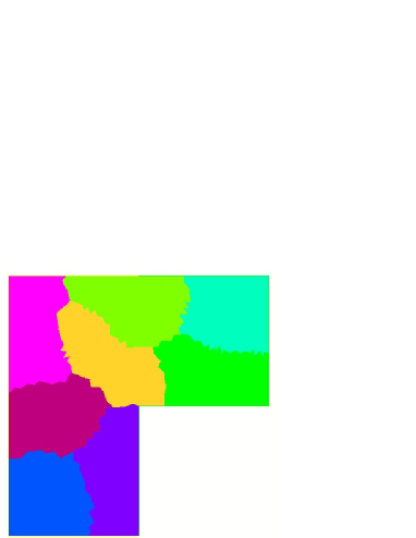
(a) L-shaped domain

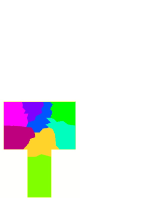
(b) T-shaped domain

Figure 2: Partition of the domain for 8 subdomains by METIS.

Let $\{\mathcal{T}_{h,i}\}_{i=1}^{N}$ be a partition of the triangulation $\mathcal{T}_{h}$ (see examples in Figure 2). For an integer value $l\geq 0$, we define an overlapping decomposition $\{\mathcal{T}_{h,i}^{l}\}_{i=1}^{N}$ such that $\mathcal{T}_{h,i}^{l}$ is a set of all triangles from $\mathcal{T}_{h,i}^{l-1}$ and all triangles from $\mathcal{T}_{h}\setminus\mathcal{T}_{h,i}^{l-1}$ that have non-empty intersection with $\mathcal{T}_{h,i}^{l-1}$, and $\mathcal{T}_{h,i}^{0}=\mathcal{T}_{h,i}$. With this definition the width of the overlap will be of $2l$. Furthermore, if $W_{h}$ stands for the finite element space associated to $\mathcal{T}_{h}$, $W_{h,i}^{l}$ is the local finite element spaces on $\mathcal{T}_{h,i}^{l}$, which is a triangulation of $\Omega_{i}$.

Let $\mathcal{N}$ be the set of indices of degrees of freedom of $W_{h}$ and $\mathcal{N}_{i}^{l}$ the set of indices of degrees of freedom of $W_{h,i}^{l}$ for $l\geq 0$. Moreover, we define the restriction operator $\mathbf{R}_{i}:W_{h}\rightarrow W_{h,i}^{l}$ as a rectangular matrix $|\mathcal{N}_{i}^{l}|\times|\mathcal{N}|$ such that if $\boldsymbol{V}$ is the vector of degrees of freedom of $v_{h}\in W_{h}$, then $\mathbf{R}_{i}\boldsymbol{V}$ is the vector of degrees of freedom of $W_{h,i}^{l}$ in $\Omega_{i}$. The extension operator from $W_{h,i}^{l}$ to $W_{h}$ and its associated matrix are both given by $\mathbf{R}_{i}^{T}$. In addition we introduce a partition of unity $\mathbf{D}_{i}$ as a diagonal matrix $|\mathcal{N}_{i}^{l}|\times|\mathcal{N}_{i}^{l}|$ such that

(4.21) $$\mathbf{Id}=\sum_{i=1}^{N}\mathbf{R}_{i}^{T}\mathbf{D}_{i}\mathbf{R}_{i},$$

where $\mathbf{Id}\in\mathbb{R}^{|\mathcal{N}|\times|\mathcal{N}|}$ is the identity matrix.

We first recall the Modified Restricted Additive Schwarz (MRAS) preconditioner introduced in [BBD⁺16] for the Stokes equation. This preconditioner is given by

(4.22) $$\mathbf{M}^{-1}_{MRAS}=\sum_{i=1}^{N}\mathbf{R}_{i}^{T}\mathbf{D}_{i}\mathbf{B}_{i}^{-1}\mathbf{R}_{i},$$

where $\mathbf{B}_{i}$ is the matrix associated to a discretisation of Stokes equation (2.1) in $\Omega_{i}$ where we impose either TVNF (2.3) or NVTF (2.4) boundary conditions in $\Omega_{i}$. In case of a discretisation of elasticity equation (2.5) in $\Omega_{i}$, we impose either TDNNS (2.7) or NDTNS (2.8) boundary conditions in $\Omega_{i}$.

We new introduce a symmetrised variant of (4.22) called Symmetrised Modified Restricted Additive Schwarz (SMRAS), given by

(4.23) $$\mathbf{M}^{-1}_{SMRAS}=\sum_{i=1}^{N}\mathbf{R}_{i}^{T}\mathbf{D}_{i}\mathbf{B}_{i}^{-1}\mathbf{D}_{i}\mathbf{R}_{i}.$$

4.1 Two-level methods

A two-level version of the SMRAS and MRAS preconditioners will be based on a spectral coarse space obtained by solving the following local generalised eigenvalue problems

Find $\left(\boldsymbol{V}_{jk},\lambda_{jk}\right)\in\mathbb{R}^{|\mathcal{N}_{j}|}\setminus\{0\}\times\mathbb{R}$ s.t.

(4.24) $$\mathbf{\tilde{A}}_{j}\boldsymbol{V}_{jk}=\lambda_{jk}\mathbf{B}_{j}\boldsymbol{V}_{jk},$$

where $\mathbf{\tilde{A}}_{j}$ are local matrices associated to a discretisation of local Neumann boundary value problem in $\Omega_{j}$. Let $\theta>0$ be a user-defined threshold. We define $Z_{GenEO}\subset\mathbb{R}^{|\mathcal{N}|}$ as the vector space spanned by the family of vectors $\left(\mathbf{R}_{j}^{T}\mathbf{D}_{j}\boldsymbol{V}_{jk}\right)_{\lambda_{jk}<\theta}$, $1\leq j\leq N$, corresponding to eigenvalues smaller than $\theta$. The value of $\theta$ is chosen such that for a given problem and preconditioner, the behaviour of the method should be robust in the sense that, its convergence should not depend, or depends very weakly, on the number of subdomains.

We are now ready to introduce the two-level method with coarse space $Z_{GenEO}$. Let $\mathbf{P}_{0}$ be the $\mathbf{A}$-orthogonal projection onto the coarse space $Z_{GenEO}$. The two-level SMRAS preconditioner is defined as

(4.25) $$\mathbf{M}^{-1}_{SMRAS,2}=\mathbf{P}_{0}\mathbf{A}^{-1}+(\mathbf{Id}-\mathbf{P}_{0})\mathbf{M}^{-1}_{SMRAS}(\mathbf{Id}-\mathbf{P}_{0}^{T}).$$

Furthermore, if $\mathbf{R}_{0}$ is a matrix whose rows are a basis of the coarse space $Z_{GenEO}$, then

$$\mathbf{P}_{0}\mathbf{A}^{-1}=\mathbf{R}_{0}^{T}\left(\mathbf{R}_{0}\mathbf{AR}_{0}^{T}\right)^{-1}\mathbf{R}_{0}.$$

In similar way, we can introduce the two-level MRAS preconditioner

(4.26) $$\mathbf{M}^{-1}_{MRAS,2}=\mathbf{P}_{0}\mathbf{A}^{-1}+(\mathbf{Id}-\mathbf{P}_{0})\mathbf{M}^{-1}_{MRAS}(\mathbf{Id}-\mathbf{P}_{0}^{T}).$$

5 Numerical results for two dimensional problems

In this section we assess the performance of the preconditioners defined in Section 4.1. We will compare the newly introduced ones with that of ORAS and SORAS introduced in [HJN15]. These kind of preconditioners are associated with the Robin interface conditions and require an optimised parameter as it can be seen in (5.27) below. The big advantage of SMRAS and MRAS preconditioners from the previous section is that they are parameter-free. We consider the partial differential equation model for nearly incompressible elasticity and Stokes flow as problems of similar mixed formulation. Each of these problems is discretised by using the Taylor-Hood methods from Section 3.1 and the hdG discretisation from Section 3.2.

Our experiments will be based on the classical weak scaling test. This test is built as follows. A domain $\bar{\Omega}$ is split into a triangulation $\mathcal{T}_{h}$. For each of element $K\in\mathcal{T}_{h}$, $h_{K}=\mbox{diam}(K)$, and we denote the mesh size by $h:=\max_{K\in\mathcal{T}_{h}}h_{K}$. Then, this triangulation is split into overlapping subdomains of size H, in such a way $\frac{H}{h}$ remains constant. In the absence of a second level in the preconditioner, if the number of subdomains grows, then the convergence gets slower. A coarse space provides a global information and leads to a more robust behaviour.

The simplest way to build a coarse space is to consider the zero energy modes. More precisely they are the eigenvectors associated with the zero eigenvalues of (4.24) on a floating subdomains. Hence, by a floating subdomain we mean a subdomain without Dirichlet boundary condition on any part of the boundary. Then the matrix on the left hand side of (4.24) is singular and there are zero eigenvalues. These zero energy modes are the rigid body motions (three in two dimensions, six in three dimensions) for the elasticity problem, and the constants (two in two dimensions, three in three dimensions) for the Stokes equations. Unfortunately for some cases, this choice is not sufficient, so we have collected the smallest $M$ eigenvalues for each subdomain and build a coarse space by including the eigenvectors associated to them. The different values of $M$ are presented in the table in brackets.

All experiments have been made by using FreeFem++ [Hec12], which is a free software specialised in variational discretisations of partial differential equations. We use GMRES [SS86] as an iterative solver. Generalized eigenvalue problems to generate the coarse space are solved using ARPACK [LSY98]. The overlapping decomposition into subdomains can be uniform (Unif) or generated by METIS (MTS) [KK98]. In each of the examples in this section we consider decomposition with two layers of mesh size $h$ in the overlap. Tables show the number of iterations needed to achieve a relative $l^{2}$ norm of the error smaller than $10^{-6}$, $\frac{\|\boldsymbol{U}-\boldsymbol{U}_{n}\|_{l^{2}}}{\|\boldsymbol{U}-\boldsymbol{U}_{0}\|_{l^{2}}}<10^{-6}$, where $\boldsymbol{U}$ is the solution of global problem given by direct solver and $\boldsymbol{U}_{m}$ denotes $m$-th iteration of the iterative solver. In addition, $DOF$ stands for number of degrees of freedom and $N$ for the number of subdomains in all tables.

5.1 Taylor-Hood discretisation

In this section we consider the Taylor-Hood discretisation from Section 3.1 with different values of $k\geq 2$ for nearly incompressible elasticity and Stokes equations.

5.1.1 Nearly incompressible elasticity

Since we consider the preconditioners with various interface conditions we need to comment the way of imposing them. ORAS and SORAS preconditioners follow [HJN15] and use Robin interface conditions. This means, the weak formulation of the linear elasticity problem contains the following term

(5.27) $$\int_{\partial\Omega_{i}\setminus\Gamma}\boldsymbol{\sigma}^{sym}_{\boldsymbol{n}}\left(\boldsymbol{v_{h}}\right)_{n}\ ds+\int_{\partial\Omega_{i}\setminus\Gamma}2\alpha\frac{\mu(2\mu+\lambda)}{\lambda+3\mu}\boldsymbol{u_{h}}\boldsymbol{v_{h}}\ ds$$

where again, following [HJN15] we choose $\alpha=10$. Fortunately, the MRAS and SMRAS preconditioners are parameter-free. For all numerical experiments associated in this section we use zero as an initial guess for the GMRES iterative solver. Moreover, the overlapping decomposition into subdomains is generated by METIS.

(a) Domain and boundary

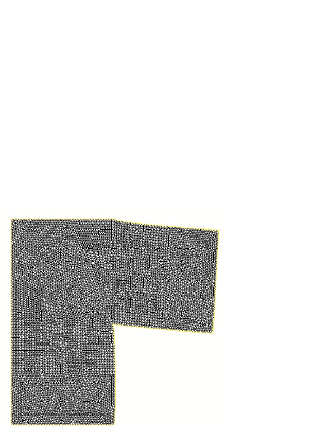
(b) Discrete solution

Figure 3: L-shaped domain problem.

Test case 1 (The L-shaped domain problem).

We consider the L-shaped domain $\Omega=(-1,1)^{2}\setminus\left\{(0,1)\times(-1,0)\right\}$ clamped on the left side and partly from a top and bottom as it is depicted in Figure 3a. This example is similar to the one in [CS15]. The associated boundary value problem is

(5.28) $$\left\{\begin{array}[]{rclclr}-2\mu\nabla\cdot\boldsymbol{\varepsilon}(\boldsymbol{u})&+&\nabla p&=&(0,-1)^{T}&\mbox{in }\Omega\\ &-&\nabla\cdot\boldsymbol{u}&=&\frac{1}{\lambda}p&\mbox{in }\Omega\\ &&\boldsymbol{u}(x,y)&=&(0,0)^{T}&\mbox{on }\Gamma_{D}\\ &&\boldsymbol{\sigma}^{sym}_{\boldsymbol{n}}(x,y)&=&(0,0)^{T}&\mbox{on }\Gamma_{N}\end{array}\right..$$

The physical parameters are $E=10^{5}$ and $\nu=0.4999$ (nearly incompressible). In Figure 3b we plot the mesh of the bent domain.

We choose $k=3$ for the Taylor-Hood discretisation. In Figure 4 we plot the eigenvalues of one floating subdomain. The clustering of small eigenvalues of the generalised eigenvalue problem defined in (4.24) suggests the number of eigenvectors to be added to the coarse space. The three zero eigenvalues correspond to the zero energy modes.

Table 1: Comparison of preconditioners for Taylor-Hood discretisation ($\boldsymbol{TH^{3}_{h}},R^{2}_{h}$) - the L-shaped domain problem.

One-level DOF N ORAS SORAS NDTNS-MRAS NDTNS-SMRAS TDNNS-MRAS TDNNS-SMRAS 124 109 4 26 60 26 60 30 59 478 027 16 57 131 69 143 65 140 933 087 32 84 180 109 221 104 211 1 899 125 64 130 293 181 362 161 312 3 750 823 128 209 412 302 568 251 510 Two-level (3 eigenvectors) DOF N ORAS SORAS NDTNS-MRAS NDTNS-SMRAS TDNNS-MRAS TDNNS-SMRAS 124 109 4 18 40 19 36 24 41 478 027 16 37 52 40 57 46 56 933 087 32 49 57 56 67 53 66 1 899 125 64 65 64 70 75 61 74 3 750 823 128 83 64 74 77 75 72 Two-level (5 eigenvectors) DOF N ORAS SORAS NDTNS-MRAS NDTNS-SMRAS TDNNS-MRAS TDNNS-SMRAS 124 109 4 15 32 17 35 24 37 478 027 16 31 41 31 47 42 47 933 087 32 40 48 38 52 53 51 1 899 125 64 49 51 45 53 64 56 3 750 823 128 69 54 49 54 70 53 Two-level (7 eigenvectors) DOF N ORAS SORAS NDTNS-MRAS NDTNS-SMRAS TDNNS-MRAS TDNNS-SMRAS 124 109 4 14 33 16 30 24 35 478 027 16 26 41 25 38 42 44 933 087 32 31 43 25 42 49 46 1 899 125 64 39 47 30 39 59 50 3 750 823 128 58 49 30 43 61 50

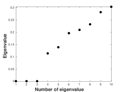
(a) Robin interface conditions

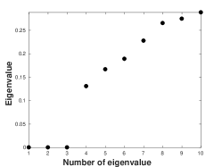
(b) NDTNS interface conditions

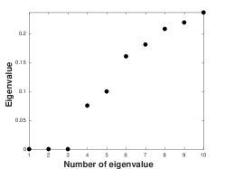
(c) TDNNS interface conditions

Figure 4: Eigenvalues on one of the floating subdomains in case of uniform decomposition and Taylor-Hood discretisation ($\boldsymbol{TH^{3}_{h}},R^{2}_{h}$) - the L-shaped domain problem.

The results of Table 1 show a clear improvement in the scalability of the two-level preconditioners over the one-level ones. In fact, using five eigenvectors per subdomain, the number of iterations is virtually unaffected by the number of subdomains. All two-level preconditioners show a comparable performance. For this case, increasing the dimension of the coarse space beyond $5\times N$ eigenvectors does not seem to improve the results dramatically.

Test case 2 (The heterogeneous beam problem).

We consider a heterogeneous beam with ten layers of steel and rubber. Five layers are made from steel with the physical parameters $E=210\cdot 10^{9}$ and $\nu=0.3$, and other five are made from rubber with the physical parameters $E=10^{8}$ and $\nu=0.4999$ as it is depicted in Figure 5a. A similar example was considered in [HJN15].

(a) Steel and rubber layers

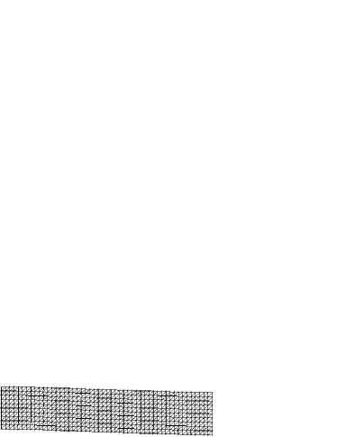
(b) Discrete solution

Figure 5: Heterogeneous beam.

The computational domain is the rectangle $\Omega=(0,5)\times(0,1)$. The beam is clamped on its left side, hence we consider the following problem

(5.29) $$\left\{\begin{array}[]{rclclr}-2\mu\nabla\cdot\boldsymbol{\varepsilon}(\boldsymbol{u})&+&\nabla p&=&(0,-1)^{T}&\mbox{in }\Omega\\ &-&\nabla\cdot\boldsymbol{u}&=&\frac{1}{\lambda}p&\mbox{in }\Omega\\ &&\boldsymbol{u}(x,y)&=&(0,0)^{T}&\mbox{on }\partial\Omega\cap\{x=0\}\\ &&\boldsymbol{\sigma}^{sym}_{\boldsymbol{n}}(x,y)&=&(0,0)^{T}&\mbox{on }\partial\Omega\setminus\{x=0\}\end{array}\right..$$

In Figure 5b we plot the mesh of the bent beam. Because of the heterogeneity of the problem, we do not notice a clear clustering of the eigenvalues (see Figure 6). In such case it is well known that coarse space including only three zero energy modes is not sufficient [DNSS12]. That is why we consider a coarse space built using 5 or 7 eigenvectors per subdomain.

Table 2: Comparison of preconditioners for Taylor-Hood discretisation ($\boldsymbol{TH^{3}_{h}},R^{2}_{h}$) - the heterogeneous beam.

One-level DOF N ORAS SORAS NDTNS-MRAS NDTNS-SMRAS TDNNS-MRAS TDNNS-SMRAS 44 963 8 168 301 160 267 177 264 87 587 16 226 490 245 462 229 424 177 923 32 373 711 447 684 440 672 347 651 64 615 $>$1000 728 $>$1000 746 $>$1000 707 843 128 973 $>$1000 $>$1000 $>$1000 $>$1000 $>$1000 1 385 219 256 $>$1000 $>$1000 $>$1000 $>$1000 $>$1000 $>$1000 Two-level (5 eigenvectors) DOF N ORAS SORAS NDTNS-MRAS NDTNS-SMRAS TDNNS-MRAS TDNNS-SMRAS 44 963 8 109 160 136 147 148 136 87 587 16 136 204 192 200 181 184 177 923 32 193 291 296 275 326 276 347 651 64 260 304 363 282 491 299 707 843 128 412 356 420 369 601 346 1 385 219 256 379 414 448 400 711 317 Two-level (7 eigenvectors) DOF N ORAS SORAS NDTNS-MRAS NDTNS-SMRAS TDNNS-MRAS TDNNS-SMRAS 44 963 8 76 118 124 115 133 103 87 587 16 106 146 166 138 159 123 177 923 32 157 202 203 185 302 214 347 651 64 178 191 225 170 326 182 707 843 128 140 114 153 112 266 122 1 385 219 256 119 86 118 77 259 94

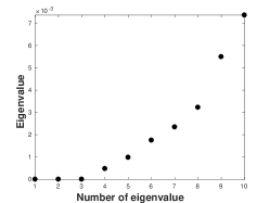
(a) Robin interface conditions

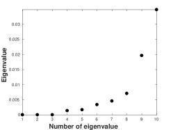
(b) NDTNS interface conditions

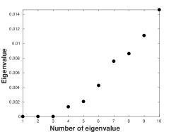
(c) TDNNS interface conditions

Figure 6: Eigenvalues on one of the floating subdomains in case of METIS decomposition and Taylor-Hood discretisation ($\boldsymbol{TH^{3}_{h}},R^{2}_{h}$) - the heterogeneous beam.

As in the previous example, the introduction of a coarse space provides a significant improvement in the number of iterations needed for convergence. Due to the high heterogeneity of this problem, more eigenvectors per subdomain are needed to obtain scalable results. We notice an important improvement of the convergence when using two-level methods (see Table 2). Although we get a stable number of iterations only when considering a coarse space which is sufficiently big.

5.1.2 Stokes equation

We now turn to the Stokes discrete problem given in Sections 3.1. Once again in case of ORAS and SORAS we choose $\alpha=10$ as in [HJN15] for the Robin interface conditions (5.27). In the first case we consider a random initial guess for the GMRES iterative solver. Later with the second example we use zero as an initial guess.

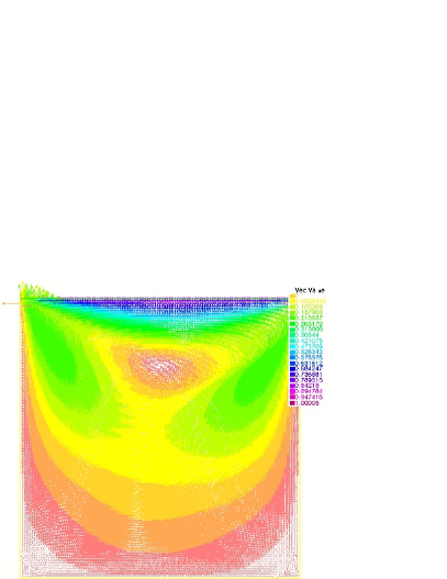
(a) Velocity field

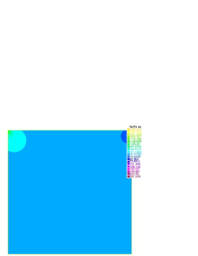
(b) Pressure

Figure 7: Numerical solution of the driven cavity problem - the driven cavity problem.

Test case 3 (The driven cavity problem).

The test case is the driven cavity. We consider the following problem on the unit square $\Omega=(0,1)^{2}$

(5.30) $$\left\{\begin{array}[]{rclclr}-\Delta\boldsymbol{u}&+&\nabla p&=&\boldsymbol{f}&\mbox{in }\Omega\\ &-&\nabla\cdot\boldsymbol{u}&=&0&\mbox{in }\Omega\\ &&\boldsymbol{u}(x,y)&=&(1,0)^{T}&\mbox{on }\partial\Omega\cap\{y=1\}\\ &&\boldsymbol{u}(x,y)&=&(0,0)^{T}&\mbox{on }\partial\Omega\setminus\{y=1\}\end{array}\right..$$

In Figure 7 we plot the vector field and pressure, after solving numerically the problem.

We start with the two energy modes only (see Figure 8). This already provides some improvement. Then, we add more eigenvectors to see if they bring improvement.

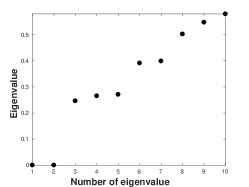
(a) Robin interface conditions

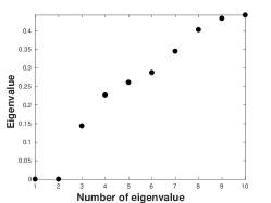
(b) NVTF interface conditions

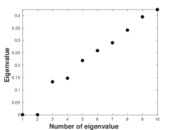
(c) TVNF interface conditions

Figure 8: Eigenvalues on one of the floating subdomains in case of uniform decomposition and Taylor-Hood discretisation ($\boldsymbol{TH^{2}_{h}},R^{1}_{h}$) - the driven cavity problem.

Table 3: Comparison of preconditioners for Taylor-Hood discretisation ($\boldsymbol{TH^{2}_{h}},R^{1}_{h}$) - the driven cavity problem.

One-level DOF N ORAS SORAS NVTF-MRAS NVTF-SMRAS TVNF-MRAS TVNF-SMRAS Unif MTS Unif MTS Unif MTS Unif MTS Unif MTS Unif MTS 91 003 4 12 17 24 34 22 22 34 40 22 25 30 40 362 003 16 28 35 56 67 52 53 90 106 54 53 70 84 813 003 36 39 75 92 103 85 91 165 185 91 88 118 136 1 444 003 64 53 91 120 144 120 135 254 283 132 132 169 206 2 728 003 121 80 278 180 212 182 280 412 580 199 213 251 439 5 768 003 256 $>$1000 $>$1000 271 317 303 452 917 955 322 319 397 695 Two-level (2 eigenvectors) DOF N ORAS SORAS NVTF-MRAS NVTF-SMRAS TVNF-MRAS TVNF-SMRAS Unif MTS Unif MTS Unif MTS Unif MTS Unif MTS Unif MTS 91 003 4 10 14 18 22 19 17 26 30 27 20 21 26 362 003 16 20 25 32 37 33 34 50 62 60 40 42 51 813 003 36 27 33 36 44 47 49 62 86 79 53 59 63 1 444 003 64 31 42 38 53 104 66 85 114 85 52 62 79 2 728 003 121 39 103 39 51 74 81 85 133 92 86 62 93 5 768 003 256 300 849 46 54 109 108 146 132 91 78 63 90 Two-level (5 eigenvectors) DOF N ORAS SORAS NVTF-MRAS NVTF-SMRAS TVNF-MRAS TVNF-SMRAS Unif MTS Unif MTS Unif MTS Unif MTS Unif MTS Unif MTS 91 003 4 9 12 13 16 16 15 18 20 25 20 16 18 362 003 16 16 20 21 24 27 22 28 37 56 37 26 35 813 003 36 23 27 25 26 33 30 39 40 65 41 28 37 1 444 003 64 26 36 27 29 40 34 35 45 77 45 28 42 2 728 003 121 35 41 29 32 43 38 34 48 84 72 29 47 5 768 003 256 66 60 32 33 56 41 60 49 88 61 29 44

The conclusions remain the same as for the L-shaped domain problem for the nearly incompressible elasticity equation discretised by Taylor-Hood method ($\boldsymbol{TH^{3}_{h}},R^{2}_{h}$) since Tables 3 and 1 show similar results.

Test case 4 (The T-shaped domain problem).

Finally, we consider a T-shaped domain $\Omega=(0,1.5)\times(0,1)\cup(0.5,1)\times(-1,1)$, and we impose mixed boundary conditions given by

(5.31) $$\boldsymbol{u}(x,y)=\left\{\begin{array}[]{c l}(4y(1-y),0)^{T}&\mbox{if }x=0\mbox{ or }x=1.5\\ (0,0)^{T}&\mbox{otherwise}.\end{array}\right.$$

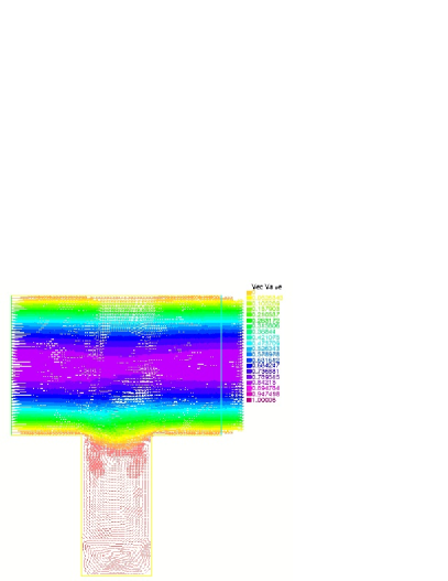
(a) Velocity field $\boldsymbol{u}$

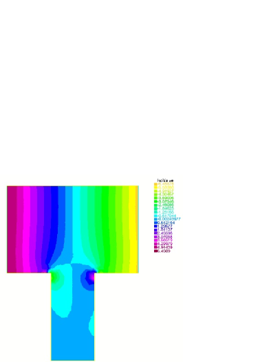
(b) Pressure $p$

Figure 9: Numerical solution - the T-shaped problem.

The numerical solution of this problem is depicted in Figure 9. The overlapping decomposition into subdomains is generated by METIS.

Once again a clustering of small eigenvalues of generalised eigenvalue problem defined in (4.24) is a motivation of the size of the coarse space (see Figure 10).

Table 4: Comparison of preconditioners for Taylor-Hood discretisation ($\boldsymbol{TH^{3}_{h}},R^{2}_{h}$) - the T-shaped problem.

One-level DOF N ORAS SORAS NVTF-MRAS NVTF-SMRAS TVNF-MRAS TVNF-SMRAS 33 269 4 13 20 12 19 13 19 138 316 16 36 51 33 52 31 45 269 567 32 59 85 52 85 49 75 553 103 64 92 132 83 136 78 115 1 134 314 128 146 208 132 223 117 188 2 201 908 256 232 328 209 357 189 293 Two-level (2 eigenvectors) DOF N ORAS SORAS NVTF-MRAS NVTF-SMRAS TVNF-MRAS TVNF-SMRAS 33 269 4 10 14 9 15 12 15 138 316 16 21 27 19 24 22 24 269 567 32 29 35 30 38 25 30 553 103 64 35 45 34 43 33 35 1 134 314 128 42 52 47 58 34 41 2 201 908 256 47 56 69 76 38 45 Two-level (5 eigenvectors) DOF N ORAS SORAS NVTF-MRAS NVTF-SMRAS TVNF-MRAS TVNF-SMRAS 33 269 4 8 13 8 13 12 14 138 316 16 15 16 14 16 20 18 269 567 32 14 19 20 22 24 19 553 103 64 16 20 18 19 29 20 1 134 314 128 17 22 23 24 30 22 2 201 908 256 16 21 34 37 35 24

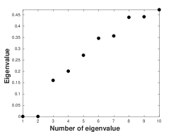
(a) Robin interface conditions

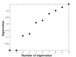
(b) NVTF interface conditions

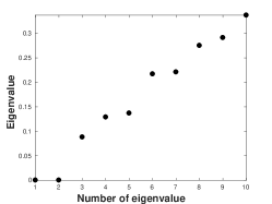
(c) TVNF interface conditions

Figure 10: Eigenvalues on one of the floating subdomains in case of METIS decomposition and Taylor-Hood discretisation ($\boldsymbol{TH^{3}_{h}},R^{2}_{h}$) - the T-shaped problem.

The same as in all examples for Taylor-Hood discretisation we notice an important improvement of the convergence when using two-level methods. Although from Table 4 we can see that the coarse spaces containing five eigenvectors seem to be sufficient.

5.2 hdG discretisation

In this section we discretise nearly incompressible elasticity equation and the Stokes flow by using the lowest order hdG discretisation introduced in Section 3.2.

5.2.1 Nearly incompressible elasticity

In case of ORAS and SORAS we consider the Robin interface conditions as in [HJN15] with $\alpha=10$. For all numerical experiments in this section we use zero as an initial guess for the GMRES iterative solver. Moreover, the overlapping decomposition into subdomains is generated by METIS.

Test case 5 (The L-shaped domain problem).

We consider the L-shaped domain discrete problem (5.28).

Table 5: Comparison of preconditioners for hdG discretisation - the L-shaped domain problem.

One-level DOF N ORAS SORAS NDTNS-MRAS NDTNS-SMRAS TDNNS-MRAS TDNNS-SMRAS 238 692 8 61 158 64 174 77 177 466 094 16 123 232 101 259 109 306 948 921 32 267 331 160 415 179 473 1 874 514 64 622 477 243 685 254 657 3 856 425 128 $>$1000 752 479 $>$1000 523 $>$1000 Two-level (3 eigenvectors) DOF N ORAS SORAS NDTNS-MRAS NDTNS-SMRAS TDNNS-MRAS TDNNS-SMRAS 238 692 8 48 98 52 98 61 116 466 094 16 89 99 71 123 75 148 948 921 32 250 130 110 158 118 173 1 874 514 64 535 135 135 155 129 159 3 856 425 128 $>$1000 152 172 176 181 192 Two-level (5 eigenvectors) DOF N ORAS SORAS NDTNS-MRAS NDTNS-SMRAS TDNNS-MRAS TDNNS-SMRAS 238 692 8 43 81 44 74 61 94 466 094 16 77 82 51 92 63 103 948 921 32 197 100 79 119 96 121 1 874 514 64 429 103 102 122 110 138 3 856 425 128 $>$1000 118 122 129 141 167 Two-level (7 eigenvectors) DOF N ORAS SORAS NDTNS-MRAS NDTNS-SMRAS TDNNS-MRAS TDNNS-SMRAS 238 692 8 35 67 38 71 44 82 466 094 16 61 79 47 80 51 95 948 921 32 153 90 58 95 74 115 1 874 514 64 423 95 71 93 72 111 3 856 425 128 934 110 79 104 108 133

Table 5 shows an important improvement of the convergence that is brought by the two-level methods. We cannot conclude that SMRAS preconditioners are much better than SORAS. Although we can note that coarse space improvement is visible for MRAS preconditioners and not for ORAS. For symmetric preconditioners (SMRAS and SORAS) five eigenvectors seem to lead already to satisfying results. While for the non-symmetric ones a bigger coarse space is required. On the other hand, we state the fact that the new preconditioners are parameter-free, which makes them easier to use as no parameter is required.

Test case 6 (The heterogeneous beam problem).

We consider the heterogeneous beam with ten layers of steel and rubber that is defined as a problem (5.29).

Table 6: Comparison of preconditioners for hdG discretisation - the heterogeneous beam.

One-level DOF N ORAS SORAS NDTNS-MRAS NDTNS-SMRAS TDNNS-MRAS TDNNS-SMRAS 46 777 8 196 440 189 402 186 463 88 720 16 317 602 330 582 326 666 179 721 32 537 $>$1000 574 $>$1000 587 $>$1000 353 440 64 899 $>$1000 847 $>$1000 846 $>$1000 704 329 128 $>$1000 $>$1000 $>$1000 $>$1000 $>$1000 $>$1000 1 410 880 256 $>$1000 $>$1000 $>$1000 $>$1000 $>$1000 $>$1000 Two-level (5 eigenvectors) DOF N ORAS SORAS NDTNS-MRAS NDTNS-SMRAS TDNNS-MRAS TDNNS-SMRAS 46 777 8 168 255 162 230 161 275 88 720 16 244 313 273 299 262 346 179 721 32 385 525 442 458 469 587 353 440 64 514 444 551 526 590 558 704 329 128 835 557 782 684 765 832 1 410 880 256 $>$1000 567 $>$1000 694 844 821 Two-level (7 eigenvectors) DOF N ORAS SORAS NDTNS-MRAS NDTNS-SMRAS TDNNS-MRAS TDNNS-SMRAS 46 777 8 148 197 149 192 158 231 88 720 16 205 201 286 187 283 273 179 721 32 318 337 385 301 433 419 353 440 64 403 262 397 247 460 389 704 329 128 490 168 447 182 558 443 1 410 880 256 $>$1000 116 387 138 473 298

We notice an improvement only when using a coarse space which is sufficiently big (see Table 6). Furthermore, we get a stable number of iterations only for the symmetric preconditioners (SMRAS and SORAS), and the coarse space improvement in case of ORAS preconditioner is much less visible than in case of MRAS preconditioners. This may be due to the fact we have not chosen an optimized parameter in the Robin interface conditions (5.27).

5.2.2 Stokes equation

We now turn to the Stokes discrete problem given in 3.2. Once again in case of ORAS and SORAS we choose $\alpha=10$ as in [HJN15] for the Robin interface conditions (5.27). In the first case we consider a random initial guess for the GMRES iterative solver. Later with the second example we use zero as an initial guess.

Test case 7 (The driven cavity problem).

We consider the driven cavity defined as a problem (5.30).

Table 7: Comparison of preconditioners for hdG discretisation - the driven cavity problem.

One-level DOF N ORAS SORAS NVTF-MRAS NVTF-SMRAS TVNF-MRAS TVNF-SMRAS Unif MTS Unif MTS Unif MTS Unif MTS Unif MTS Unif MTS 93 656 4 17 18 37 38 24 22 44 44 32 25 48 50 373 520 16 76 122 75 84 52 54 107 111 68 67 122 126 839 592 36 152 327 120 133 91 96 194 200 112 115 206 210 1 491 872 64 261 587 162 176 130 143 294 303 159 158 292 286 2 819 432 121 364 $>$1000 229 256 199 213 504 649 238 251 628 643 5 963 072 256 592 $>$1000 367 398 326 477 $>$1000 $>$1000 392 404 995 740 Two-level (2 eigenvectors) DOF N ORAS SORAS NVTF-MRAS NVTF-SMRAS TVNF-MRAS TVNF-SMRAS Unif MTS Unif MTS Unif MTS Unif MTS Unif MTS Unif MTS 93 656 4 12 14 30 28 18 18 33 32 40 23 38 37 373 520 16 81 80 47 57 36 40 61 73 100 49 85 82 839 592 36 236 228 61 60 57 65 97 104 132 66 112 107 1 491 872 64 395 463 67 71 79 85 139 129 142 70 128 122 2 819 432 121 840 $>$1000 73 86 113 127 188 178 157 86 127 139 5 963 072 256 $>$1000 $>$1000 80 87 171 179 283 287 167 108 132 148 Two-level (5 eigenvectors) DOF N ORAS SORAS NVTF-MRAS NVTF-SMRAS TVNF-MRAS TVNF-SMRAS Unif MTS Unif MTS Unif MTS Unif MTS Unif MTS Unif MTS 93 656 4 10 12 25 24 14 16 23 22 52 22 29 26 373 520 16 27 35 38 37 27 29 38 41 117 39 53 53 839 592 36 135 84 45 41 35 37 51 50 145 49 64 61 1 491 872 64 278 212 49 45 44 42 58 55 157 59 64 64 2 819 432 121 607 584 56 49 46 56 58 62 162 81 65 75 5 963 072 256 $>$1000 $>$1000 62 55 52 64 57 69 166 75 65 75

The conclusions remain the same as in the case of nearly incompressible elasticity equation for the L-shaped domain. Although Table 7 shows that coarse spaces containing five eigenvectors seem to decrease the number of iteration even in the case of MRAS preconditioners that are not fully scalable.

Test case 8 (The T-shaped domain problem).

Finally, we consider a T-shaped domain $\Omega=(0,1.5)\times(0,1)\cup(0.5,1)\times(-1,1)$, and we impose mixed boundary conditions (5.31). The numerical solution of this problem is depicted in Figure 9.

Table 8: Comparison of preconditioners for hdG discretisation - the T-shaped problem.

One-level DOF N ORAS SORAS NVTF-MRAS NVTF-SMRAS TVNF-MRAS TVNF-SMRAS 38 803 4 22 45 36 49 22 51 154 606 16 111 98 83 172 83 182 311 369 32 265 144 133 262 130 266 616 772 64 568 238 212 410 195 412 1 246 136 128 $>$1000 494 333 665 313 602 2 451 365 256 $>$1000 712 464 $>$1000 477 889 Two-level (2 eigenvectors) DOF N ORAS SORAS NVTF-MRAS NVTF-SMRAS TVNF-MRAS TVNF-SMRAS 38 803 4 16 35 31 37 21 38 154 606 16 113 69 73 75 38 75 311 369 32 254 99 103 176 93 162 616 772 64 510 153 171 273 121 140 1 246 136 128 $>$1000 221 242 252 155 138 2 451 365 256 $>$1000 286 343 515 189 231 Two-level (5 eigenvectors) DOF N ORAS SORAS NVTF-MRAS NVTF-SMRAS TVNF-MRAS TVNF-SMRAS 38 803 4 14 30 27 27 28 30 154 606 16 155 54 54 45 25 44 311 369 32 159 55 72 59 29 52 616 772 64 426 88 106 83 37 76 1 246 136 128 955 113 115 99 43 72 2 451 365 256 $>$1000 182 138 101 54 73

In this case scalable results can be only observed for the preconditioners associated with the non standard interface conditions (MRAS and SMRAS), and when using a coarse space which is sufficiently big (see Table 8). In the case of ORAS or SORAS, one possibility is to choose a different parameter $\alpha$, but the proof of this, and even the question of whether this would have a positive impact, are open problems.

6 Numerical results for three dimensional problems

In this section we again assess the performance of the preconditioners as in Section 5, but this time in case of three dimensional problems. We consider the partial differential equation model for nearly incompressible elasticity and Stokes flow as three dimensional problems of similar mixed formulation. Each of these problems is discretised by using the Taylor-Hood methods from Section 3.1. In addition, we use the same tools as in Section 5. For both test cases we use zero as an initial guess.

6.1 Taylor-Hood discretisation

In this section we consider the Taylor-Hood discretisation from Section 3.1 with $k=2$ for nearly incompressible elasticity and Stokes equations.

6.1.1 Nearly incompressible elasticity

In three dimensional space, ORAS and SORAS preconditioners also require an optimized parameter. We follow [HJN15] and use Robin interface conditions (5.27) with $\alpha=10$.

Test case 9 (The homogeneous beam problem).

We consider a homogeneous beam with the physical parameters $E=10^{8}$ and $\nu=0.4999$. The computational domain is the rectangle $\Omega=(0,5)\times(0,1)\times(0,1)$. The beam is clamped on one side, hence we consider the following problem

(6.32) $$\left\{\begin{array}[]{rclclr}-2\mu\nabla\cdot\boldsymbol{\varepsilon}(\boldsymbol{u})&+&\nabla p&=&(0,0,-1)^{T}&\mbox{in }\Omega\\ &-&\nabla\cdot\boldsymbol{u}&=&\frac{1}{\lambda}p&\mbox{in }\Omega\\ &&\boldsymbol{u}(x,y)&=&(0,0,0)^{T}&\mbox{on }\partial\Omega\cap\{x=0\}\\ &&\boldsymbol{\sigma}^{sym}_{\boldsymbol{n}}(x,y)&=&(0,0,0)^{T}&\mbox{on }\partial\Omega\setminus\{x=0\}\end{array}\right..$$

Table 9: Comparison of preconditioners for Taylor-Hood discretisation ($\boldsymbol{TH^{2}_{h}},R^{1}_{h}$) - the homogeneous beam.

One-level DOF N ORAS SORAS NDTNS-MRAS NDTNS-SMRAS TDNNS-MRAS TDNNS-SMRAS 32 446 8 21 45 29 36 27 37 73 548 16 31 70 38 64 26 67 139 794 32 43 99 74 94 66 91 299 433 64 55 143 161 140 149 139 549 396 128 78 192 314 192 229 199 Two-level (6 eigenvectors) DOF N ORAS SORAS NDTNS-MRAS NDTNS-SMRAS TDNNS-MRAS TDNNS-SMRAS 32 446 8 10 17 13 18 12 17 73 548 16 11 22 16 25 16 22 139 794 32 13 26 25 28 17 26 299 433 64 15 27 19 27 24 28 549 396 128 17 28 20 25 21 26 Two-level (8 eigenvectors) DOF N ORAS SORAS NDTNS-MRAS NDTNS-SMRAS TDNNS-MRAS TDNNS-SMRAS 32 446 8 9 16 12 17 12 16 73 548 16 10 19 15 24 14 20 139 794 32 11 21 17 23 17 21 299 433 64 14 24 17 24 21 23 549 396 128 16 27 18 23 20 22

The results of Table 9 show a clear improvement in the scalability of the two-level preconditioners over the one-level ones. In fact, using only zero energy modes, the number of iterations is virtually unaffected by the number of subdomains. All two-level preconditioners show a comparable performance. For this case, increasing the dimension of the coarse space beyond $6\times N$ eigenvectors does not seem to improve the results dramatically.

6.1.2 Stokes equation

We now turn to the Stokes discrete problem given in 3.1. Once again in case of ORAS and SORAS we choose $\alpha=10$ as in [HJN15] for the Robin interface conditions (5.27).

Test case 10 (The driven cavity problem).

The test case is the three-dimensional version of the driven cavity problem. We consider the following problem on the unit cube $\Omega=(0,1)^{3}$

(6.33) $$\left\{\begin{array}[]{rclclr}-\Delta\boldsymbol{u}&+&\nabla p&=&\boldsymbol{f}&\mbox{in }\Omega\\ &-&\nabla\cdot\boldsymbol{u}&=&0&\mbox{in }\Omega\\ &&\boldsymbol{u}(x,y)&=&(1,0,0)^{T}&\mbox{on }\partial\Omega\cap\{y=1\}\\ &&\boldsymbol{u}(x,y)&=&(0,0,0)^{T}&\mbox{on }\partial\Omega\setminus\{y=1\}\end{array}\right..$$

Table 10: Comparison of preconditioners for Taylor-Hood discretisation ($\boldsymbol{TH^{2}_{h}},R^{1}_{h}$) - the driven cavity problem.

One-level DOF N ORAS SORAS NVTF-MRAS NVTF-SMRAS TVNF-MRAS TVNF-SMRAS 38 229 8 12 24 12 22 11 23 76 542 16 18 34 18 31 15 31 158 818 32 23 45 20 45 19 45 325 293 64 28 60 36 64 25 60 643 137 128 37 79 64 91 33 88 Two-level (3 eigenvectors) DOF N ORAS SORAS NVTF-MRAS NVTF-SMRAS TVNF-MRAS TVNF-SMRAS 38 229 8 10 17 10 18 11 18 76 542 16 11 20 11 19 14 19 158 818 32 13 24 13 24 16 23 325 293 64 15 27 15 27 19 26 643 137 128 18 31 17 32 22 31 Two-level (7 eigenvectors) DOF N ORAS SORAS NVTF-MRAS NVTF-SMRAS TVNF-MRAS TVNF-SMRAS 38 229 8 9 16 9 16 12 17 76 542 16 10 17 10 18 15 17 158 818 32 11 19 11 20 17 20 325 293 64 13 19 13 21 20 20 643 137 128 15 21 16 22 22 22

The conclusions remain the same as for the homogeneous beam example for the nearly incompressible elasticity equation discretised by Taylor-Hood method ($\boldsymbol{TH^{3}_{h}},R^{2}_{h}$) since Tables 10 and 9 show similar results.

7 Conclusion

We tested numerically two-level preconditioners with spectral coarse spaces for nearly incompressible elasticity and Stokes equations. We considered two finite element methods, namely, Taylor-Hood (Section 3.1) and the hdG (Section 3.2) discretisations.

In the case of the homogeneous nearly incompressible elasticity the two-level methods coupled with SORAS preconditioner defined in [HJN15] and SMRAS preconditioner defined by (4.23) allowed us to achieve good scalability results for both discretisations. Furthermore, for these symmetric preconditioners coarse spaces containing only zero energy modes seem to be enough for two and three dimensional problems. For the heterogeneous problem we also achieved scalability for two-level SORAS and SMRAS preconditioners, but, as expected, only in the case when the size of the coarse space is sufficiently big.

The improvement of the convergence in the case of the Stokes flow is visible only when the coarse space contains more eigenvectors than only constants. For the Taylor-Hood discretisation, taking sufficient big coarse space we were able to achieve good scalability for all preconditioners. It is remarkable that these good results occur even when using the hdG discretisation, despite the fact the optimized parameter to be used in SORAS and ORAS is not available.

We can conclude that the two-level preconditioners associated with non standard interface conditions are at least as good as the two-level ones in conjunction with Robin interface conditions using optimised parameters. It shows an important advantage of newly introduced preconditioners as they are parameter-free.

Numerical tests have shown that the coarse spaces bring an important improvement in the convergence, but the size of the coarse space depends on the problem. Building as small as possible coarse spaces is important from computational point of view. Thus, it is necessary to investigate what could be an optimal criterion for choosing the eigenvectors for a coarse space.

As we mentioned before, the theoretical foundation of the two-level preconditioners has not been extended to saddle point problems. Hence, future research will be devoted to this topic.

References

- [AdDBM+14] B. Ayuso de Dios, F. Brezzi, L. D. Marini, J. Xu, and L. Zikatanov. A simple preconditioner for a discontinuous Galerkin method for the Stokes problem. Journal of Scientific Computing, 58(3):517–547, 2014.
- [BBD+16] G. R Barrenechea, M. Bosy, V. Dolean, F. Nataf, and P.-H. Tournier. Hybrid discontinuous Galerkin discretisation and preconditioning of the Stokes problem with non standard boundary conditions. preprint, https://arxiv.org/abs/1610.09207, October 2016.
- [BBF13] D. Boffi, F. Brezzi, and M. Fortin. Mixed finite element methods and applications, volume 44 of Springer Series in Computational Mathematics. Springer, Heidelberg, 2013.
- [BHMV99] M. Brezina, C. I Heberton, J. Mandel, and P. Vanek. An iterative method with convergence rate chosen a priori, ucd/ccm report 140. Technical report, Center for Computational Mathematics, University of Colorado at Denver, 1999.
- [CDKN14] L. Conen, V. Dolean, R. Krause, and F. Nataf. A coarse space for heterogeneous Helmholtz problems based on the Dirichlet-to-Neumann operator. J. Comput. Appl. Math., 271:83–99, 2014.
- [CG09] B. Cockburn and J. Gopalakrishnan. The derivation of hybridizable discontinuous Galerkin methods for Stokes flow. SIAM J. Numer. Anal., 47(2):1092–1125, 2009.
- [CGL09] B. Cockburn, J. Gopalakrishnan, and R. Lazarov. Unified hybridization of discontinuous Galerkin, mixed, and continuous Galerkin methods for second order elliptic problems. SIAM J. Numer. Anal., 47(2):1319–1365, 2009.
- [CS15] C. Carstensen and M. Schedensack. Medius analysis and comparison results for first-order finite element methods in linear elasticity. IMA J. Numer. Anal., 35(4):1591–1621, 2015.
- [DJN15] V. Dolean, P. Jolivet, and F. Nataf. An introduction to domain decomposition methods. Society for Industrial and Applied Mathematics (SIAM), Philadelphia, PA, 2015. Algorithms, theory, and parallel implementation.
- [DNSS12] V. Dolean, F. Nataf, R. Scheichl, and N. Spillane. Analysis of a two-level Schwarz method with coarse spaces based on local Dirichlet-to-Neumann maps. Comput. Methods Appl. Math., 12(4):391–414, 2012.
- [EGLW12] Y. Efendiev, J. Galvis, R. Lazarov, and J. Willems. Robust domain decomposition preconditioners for abstract symmetric positive definite bilinear forms. ESAIM Math. Model. Numer. Anal., 46(5):1175–1199, 2012.
- [GE10a] J. Galvis and Y. Efendiev. Domain decomposition preconditioners for multiscale flows in high-contrast media. Multiscale Model. Simul., 8(4):1461–1483, 2010.
- [GE10b] J. Galvis and Y. Efendiev. Domain decomposition preconditioners for multiscale flows in high contrast media: reduced dimension coarse spaces. Multiscale Model. Simul., 8(5):1621–1644, 2010.
- [GR86] V. Girault and P. A. Raviart. Finite element methods for Navier-Stokes equations, volume 5 of Springer Series in Computational Mathematics. Springer-Verlag, Berlin, 1986. Theory and algorithms.
- [Hec12] F. Hecht. New development in FreeFem++. J. Numer. Math., 20(3-4):251–265, 2012.
- [HJN15] R. Haferssas, P. Jolivet, and F. Nataf. An additive Schwarz method type theory for Lions’ algorithm and Optimized Schwarz Methods. preprint, https://hal.archives-ouvertes.fr/hal-01278347, December 2015.
- [KK98] G. Karypis and V. Kumar. A software package for partitioning unstructured graphs, partitioning meshes, and computing fill-reducing orderings of sparse matrices. Technical report, University of Minnesota, Department of Computer Science and Engineering, Army HPC Research Center, Minneapolis, MN, 1998.
- [LNS15] Sébastien Loisel, Hieu Nguyen, and Robert Scheichl. Optimized Schwarz and 2-Lagrange multiplier methods for multiscale elliptic PDEs. SIAM J. Sci. Comput., 37(6):A2896–A2923, 2015.
- [LSY98] R. B. Lehoucq, D. C. Sorensen, and C. Yang. ARPACK users’ guide, volume 6 of Software, Environments, and Tools. Society for Industrial and Applied Mathematics (SIAM), Philadelphia, PA, 1998. Solution of large-scale eigenvalue problems with implicitly restarted Arnoldi methods.
- [Nic87] R. A. Nicolaides. Deflation of conjugate gradients with applications to boundary value problems. SIAM J. Numer. Anal., 24(2):355–365, 1987.
- [NXD10] F. Nataf, H. Xiang, and V. Dolean. A two level domain decomposition preconditioner based on local Dirichlet-to-Neumann maps. C. R. Math. Acad. Sci. Paris, 348(21-22):1163–1167, 2010.
- [PS11] A. Pechstein and J. Schöberl. Tangential-displacement and normal-normal-stress continuous mixed finite elements for elasticity. Math. Models Methods Appl. Sci., 21(8):1761–1782, 2011.
- [SDH+14] N. Spillane, V. Dolean, P. Hauret, F. Nataf, C. Pechstein, and R. Scheichl. Abstract robust coarse spaces for systems of PDEs via generalized eigenproblems in the overlaps. Numer. Math., 126(4):741–770, 2014.
- [SS86] Y. Saad and M. H. Schultz. GMRES: a Generalized Minimal Residual algorithm for solving nonsymmetric linear systems. SIAM J. Sci. Statist. Comput., 7(3):856–869, 1986.
- [TW05] A. Toselli and O. Widlund. Domain Decomposition Methods - Algorithms and Theory, volume 34 of Springer Series in Computational Mathematics. Springer, 2005.