Oscillation phenomena and experimental determination of exact mathematical Stability Zones for magneto-conductivity in metals having complicated Fermi surfaces.

Abstract

We consider the problem of exact experimental determination of the boundaries of Stability Zones for magneto-conductivity in normal metals in the space of directions of $\,{\bf B}\,$. As can be shown, this problem turns out to be nontrivial since the exact boundaries of Stability Zones are in fact unobservable in direct measurements of conductivity. However, this problem can be effectively solved with the aid of the study of oscillation phenomena (cyclotron resonance, quantum oscillations) in normal metals, which reveal a singular behavior on the mathematical boundary of a Stability Zone.

I Introduction.

In this paper we consider galvano-magnetic phenomena in normal metals, having complicated Fermi surfaces, in the limit of the strong magnetic fields $\,{\bf B}\,\,$ ($\omega_{B}\tau\,\gg\,1$). In the standard approach we assume that the electron states are described by a single-particle partition function $\,f({\bf p})\,$ defined on the space of the quasimomenta $\,{\bf p}\,\in\,\mathbb{T}^{3}\,$ for a given type of the crystal lattice of a metal. In the equilibrium state we assume as usually that all the electron states with energy $\,\epsilon({\bf p})\,$ less than the Fermi energy are occupied ($f({\bf p})=1$) and all the states with energy higher than the Fermi energy are empty ($f({\bf p})=0$). Let us say also that we will omit here the spin variables which will not play an essential role in our consideration.

The space of the quasimomenta $\,{\bf p}\,$ for a given conduction band represents a three-dimensional torus $\,\mathbb{T}^{3}\,$ given by the factorization of the space $\,\mathbb{R}^{3}\,$ over the reciprocal lattice vectors

$$\mathbb{T}^{3}\,\,\,\,=\,\,\,\,\left.\mathbb{R}^{3}\,\right/\,\left\{n_{1}{\bf a}_{1}\,+\,n_{2}{\bf a}_{2}\,+\,n_{3}\,{\bf a}_{3}\right\}\quad,\\ n_{1}\,,\,\,n_{2}\,,\,\,n_{3}\,\,\,\in\,\,\,\mathbb{Z}$$

The vectors $\,({\bf a}_{1},\,{\bf a}_{2},\,{\bf a}_{3})\,$ represent a basis for the reciprocal lattice and are connected with the basis vectors $\,({\bf l}_{1},\,{\bf l}_{2},\,{\bf l}_{3})\,$ of the direct lattice by standard relations

$${\bf a}_{1}\,\,\,=\,\,\,2\pi\hbar\,\,{{\bf l}_{2}\,\times\,{\bf l}_{3}\over({\bf l}_{1},\,{\bf l}_{2},\,{\bf l}_{3})}\,\,\,,\quad\quad{\bf a}_{2}\,\,\,=\,\,\,2\pi\hbar\,\,{{\bf l}_{3}\,\times\,{\bf l}_{1}\over({\bf l}_{1},\,{\bf l}_{2},\,{\bf l}_{3})}\,\,\,,$$

$${\bf a}_{3}\,\,\,=\,\,\,2\pi\hbar\,\,{{\bf l}_{1}\,\times\,{\bf l}_{2}\over({\bf l}_{1},\,{\bf l}_{2},\,{\bf l}_{3})}$$

In this approach the Fermi surface $\,S_{F}\,$:

$$S_{F}\quad:\quad\epsilon({\bf p})\,=\,\epsilon_{F}$$

represents a compact smooth surface embedded into three-dimensional torus $\,\mathbb{T}^{3}\,$.

Equivalently, we can consider the whole space of the quasimomenta ($\mathbb{R}^{3}$) and assume that any two values of $\,{\bf p}\,$ which differ by a reciprocal lattice vector represent the same physical state for a given conduction band. In this approach the dispersion relation $\,\epsilon({\bf p})\,$ should be considered as a three-periodic function in $\,\mathbb{R}^{3}\,$ with the periods $\,{\bf a}_{1}\,$, $\,{\bf a}_{2}\,$, and $\,{\bf a}_{3}\,$. The Fermi surface represents in this case a three-periodic surface in $\,\mathbb{R}^{3}\,$ which can have in general a rather complicated form (see e.g. Fig. 1).

Figure 1: A complicated Fermi surface as a 3-periodic surface in the ${\bf p}$ - space.

In the quasiclassical approximation the evolution of the electron states in metal in the presence of electric and magnetic fields can be described by the adiabatic system

$${\dot{\bf p}}\,\,\,\,=\,\,\,\,{e\over c}\,\,\left[{\bf v}_{\rm gr}({\bf p})\,\times\,{\bf B}\right]\,\,\,+\,\,\,e\,{\bf E}$$

In the limit of the strong magnetic fields the behavior of conductivity is actually defined by the geometry of the dynamical system

$${\dot{\bf p}}\,\,\,\,=\,\,\,\,{e\over c}\,\,\left[{\bf v}_{\rm gr}({\bf p})\,\times\,{\bf B}\right]\,\,\,\,=\,\,\,\,{e\over c}\,\,\left[\nabla\epsilon({\bf p})\,\times\,{\bf B}\right]$$ (I.1)

which will play the basic role in our considerations here.

System (I.1) is integrable from analytical point of view and its trajectories are given by the intersections of the constant energy levels $\,\epsilon({\bf p})\,=\,{\rm const}\,$ with the planes, orthogonal to $\,{\bf B}$. At the same time, the global geometry of the trajectories of (I.1) can still be rather nontrivial in the ${\bf p}$ - space, which can be seen if we consider an intersection of a complicated Fermi surface by an arbitrary plane (Fig. 2).

Figure 2: An intersection of a complicated Fermi surface by a plane of general direction in the ${\bf p}$ - space.

An important role of the geometry of open trajectories of system (I.1) for the behavior of conductivity in strong magnetic fields was first revealed by the school of I.M. Lifshitz (I.M. Lifshitz, M.Ya. Azbel, M.I. Kaganov, V.G. Peschasky) in 1950’s (see lifazkag ; lifpes1 ; lifpes2 ; lifkag1 ; lifkag2 ; lifkag3 ; etm ; KaganovPeschansky ). Thus, in the paper lifazkag the crucial difference between the contribution of the closed and open periodic trajectories (Fig. 3) of (I.1) to the conductivity tensor in the limit $\,\omega_{B}\tau\,\rightarrow\,\infty\,$ was first described.

Figure 3: Closed (a) and open periodic (b) electron trajectories on the Fermi surfaces of different forms.

In papers lifpes1 ; lifpes2 more general types of open trajectories, which are not periodic in ${\bf p}$ - space and are locally stable with respect to small rotations of $\,{\bf B}\,$ were considered. Both the open periodic trajectories of (I.1) and more general trajectories, considered in lifpes1 ; lifpes2 , have a mean direction in the ${\bf p}$ - space which results in strong anisotropy of their contribution to the conductivity in the plane orthogonal to $\,{\bf B}\,$. Thus, if we chose the $z$ - axis along the direction of $\,{\bf B}\,$ and the $x$ - axis along the mean direction of the open trajectories in ${\bf p}$ - space we can write for the limiting values of the conductivity tensor $\,\sigma^{kl}(B)\,$:

$$\sigma^{kl}_{\infty}\,\,\,\,=\,\,\,\,{ne^{2}\tau\over m^{*}}\,\,\left(\begin{array}[]{ccc}0&0&0\cr 0&*&*\cr 0&*&*\end{array}\right)$$ (I.2)

In formula (I.2) the value $\,n\,$ denotes the mean concentration of the conductivity electrons in metal and $\,m^{*}\,$ has a meaning of the effective electron mass in the crystal. The value $\,\tau\,$ has a meaning of the mean free electron motion time, and $\,*\,$ denote just some dimensionless constants of order of unity. Let us note that the projection of a quasiclassical electron trajectory in ${\bf x}$ - space on the plane orthogonal to $\,{\bf B}\,$ coincides with the corresponding trajectory in ${\bf p}$ - space, rotated by $90^{\circ}$, which explains the form of the tensor (I.2). It’s not difficult to see that the measurement of the conductivity in the plane orthogonal to $\,{\bf B}\,$ gives a possibility to find the mean direction of the open trajectories in ${\bf p}$ - space, which coincides with the direction of the lowest conductivity in the limit $\,\omega_{B}\tau\,\rightarrow\,\infty\,$.

For comparison, the contribution of the closed trajectories of system (I.1) to the conductivity tensor is almost isotropic in the plane orthogonal to $\,{\bf B}\,$ in the limit $\,\omega_{B}\tau\,\rightarrow\,\infty\,$ and we can write for its limiting values

$$\sigma^{kl}_{\infty}\,\,\,\,=\,\,\,\,{ne^{2}\tau\over m^{*}}\,\,\left(\begin{array}[]{ccc}0&0&0\cr 0&0&0\cr 0&0&*\end{array}\right)\quad,$$

where $\,\,{\hat{z}}\,=\,{\bf B}/B$.

The general problem of classification of different trajectories of system (I.1) with arbitrary periodic dispersion relation $\,\epsilon({\bf p})\,$ was set by S.P. Novikov (MultValAnMorseTheory ) and was intensively studied in his topological school (S.P. Novikov, A.V. Zorich, S.P. Tsarev, I.A. Dynnikov). Let us say here, that this problem turned out to be highly non-trivial in its general form and required a set of rather deep topological results for its complete investigation (see zorich1 ; dynn1992 ; Tsarev ; dynn1 ; dynn2 ). The most important achievements in the study of this problem were made in the papers zorich1 ; dynn1 where deep topological theorems about the behavior of trajectories of system (I.1) were proved. In particular, the results obtained in zorich1 and dynn1 give a basis for description of the stable (regular) non-closed trajectories of system (I.1) with arbitrary $\,\epsilon({\bf p})\,$ which will be also considered in the present paper. Let us formulate here the properties of the stable (with respect to small rotations of $\,{\bf B}\,$ or small variations of the Fermi energy $\,\epsilon_{F}$) open trajectories of system (I.1), which play, from our point of view, the most important role in the magneto-transport phenomena in normal metals:

1) Every stable open trajectory of system (I.1) lies in a straight strip of a finite width in the plane orthogonal to $\,{\bf B}\,$ and passes through it from $\,-\infty\,$ to $\,+\infty\,$ (Fig. 4);

2) All the stable open trajectories at a given direction of $\,{\bf B}\,$ have the same mean direction in ${\bf p}$ - space, which is given by the intersection of the plane, orthogonal to $\,{\bf B}\,$, and some locally stable integral plane in the ${\bf p}$ - space.

Figure 4: The form of a stable open trajectory of system (I.1) in the plane orthogonal to $\,{\bf B}\,$.

The properties formulated above were used in PismaZhETF for the introduction of important topological characteristics of electron spectra in metals observable in the transport phenomena in strong magnetic fields. These characteristics were called in PismaZhETF the topological quantum numbers observable in the conductivity of normal metals and can be described in the following way:

First, according to property (1) we should observe a strong anisotropy of conductivity in the plane orthogonal to $\,{\bf B}\,$ in the limit $\,\omega_{B}\tau\,\rightarrow\,\infty\,$ in the case of presence of stable open trajectories on the Fermi surface. The limiting values of the conductivity tensor $\,\sigma^{kl}(B)\,$ are given by the formula (I.2) and we can define the mean direction of the open trajectories of (I.1) as the direction of the lowest conductivity in the plane orthogonal to $\,{\bf B}\,$ for $\,\omega_{B}\tau\gg 1$. Due to the stability properties of the open trajectories we can define also these directions for close directions of $\,{\bf B}\,$ and define an integral plane $\,\Gamma\,$, which is swept by the directions of the lowest conductivity in a given “Stability Zone” in the space of directions of $\,{\bf B}\,$.

Let us mention here that integral character of the plane $\,\Gamma\,$ in the ${\bf p}$ - space means that it is generated by some two reciprocal lattice vectors $\,{\bf q}_{1}$, $\,{\bf q}_{2}$:

$$\begin{array}[]{c}\Gamma\,\,\,=\,\,\,\{\lambda\,{\bf q}_{1}\,\,+\,\,\mu\,{\bf q}_{2}\,,\quad\lambda,\mu\,\in\,\mathbb{R}\}\,\,\,,\\ \\ {\bf q}_{1}\,\,=\,\,n_{1}{\bf a}_{1}\,+\,n_{2}{\bf a}_{2}\,+\,n_{3}{\bf a}_{3}\,\,\,,\\ \\ {\bf q}_{2}\,\,=\,\,m_{1}{\bf a}_{1}\,+\,m_{2}{\bf a}_{2}\,+\,m_{3}{\bf a}_{3}\,\,\,,\\ \\ (n_{1},n_{2},n_{3},m_{1},m_{2},m_{3}\,\in\,\mathbb{Z})\end{array}$$

In the ${\bf x}$ - space the plane $\,\Gamma\,$ can be given by an indivisible triple of integers $\,(M_{1},M_{2},M_{3})\,$ from the equation

$$M_{1}\,\left({\bf x},{\bf l}_{1}\right)\,\,+\,\,M_{2}\,\left({\bf x},{\bf l}_{2}\right)\,\,+\,\,M_{3}\,\left({\bf x},{\bf l}_{3}\right)\,\,\,=\,\,\,0$$

where $\,({\bf l}_{1},{\bf l}_{2},{\bf l}_{3})\,$ represent the basis of the direct lattice. The numbers $\,(M_{1},M_{2},M_{3})\,$ were called in PismaZhETF the topological quantum numbers observable in conductivity of normal metals and represent the homology classes of two-dimensional “carriers of open trajectories” in the torus $\,\mathbb{T}^{3}\,$. Let us say that the triples $\,(M_{1},M_{2},M_{3})\,$ can be rather nontrivial for complicated Fermi surfaces and represent (together with the geometry of the “Stability Zones”) an important characteristic of the electron spectrum in a metal.

Another important property of the stable open trajectories of system (I.1) is that they never appear together with more complicated (unstable) chaotic open trajectories (chaotic trajectories of Tsarev or Dynnikov type) at the same direction of $\,{\bf B}\,$ (dynn3 ). As a result, the contribution of the trajectories shown at Fig. 4 to the conductivity represents the only nontrivial part of the tensor $\,\sigma^{kl}({\bf B})\,$ in the “Stability Zone” and is easily observable in experiments. Let us say here also, that the consideration of “chaotic” trajectories of system (I.1) will not be a subject of the present paper.

The most detailed mathematical survey on the geometry of trajectories of system (I.1) is represented in the paper dynn3 . The detailed description of the physical phenomena based on topological investigations of the system (I.1) can be found in the papers UFN ; BullBrazMathSoc ; JournStatPhys . Let us give also a reference to the paper DeLeoPhysB where a convenient mathematical method of numerical investigation of the structure of Stability Zones, suggested by I.A. Dynnikov, was used by R. De Leo for investigation of Stability Zones for a set of analytical dispersion relations, used as approximations to dispersion relations in real crystals. We can give here also a reference to the papers dynn2 ; zorich2 ; ZhETF1997 ; DeLeo1 ; DeLeo2 ; DeLeo3 ; DeLeoDynnikov1 ; DeLeoDynnikov2 ; Skripchenko1 ; Skripchenko2 ; DynnSkrip devoted to investigation of different aspects of chaotic trajectories of system (I.1), which can arise on rather complicated Fermi surfaces.

The present paper will be devoted to the methods of experimental determination of the boundaries of exact mathematical “Stability Zones”, which represents in fact a nontrivial problem from experimental point of view. Let us say at once that we define the exact mathematical Stability Zone $\,\Omega_{\alpha}\,$ as a region on the angle diagram (unit sphere $\,\mathbb{S}^{2}\,$) corresponding to the presence of the stable open trajectories with the same topological quantum numbers $\,(M^{\alpha}_{1},M^{\alpha}_{2},M^{\alpha}_{3})\,$ on the Fermi surface. According to this definition, the open trajectories of system (I.1) exist for any $\,{\bf B}/B\,\in\,\Omega_{\alpha}\,$, are stable with respect to small rotations of $\,{\bf B}\,$ and define the same integral plane $\,\Gamma_{\alpha}\,$ in the ${\bf p}$ - space. The Stability Zone $\,\Omega_{\alpha}\,$, defined in this way, represents a finite region on the unit sphere $\,\mathbb{S}^{2}\,$ with a piecewise smooth boundary (Fig. 5).

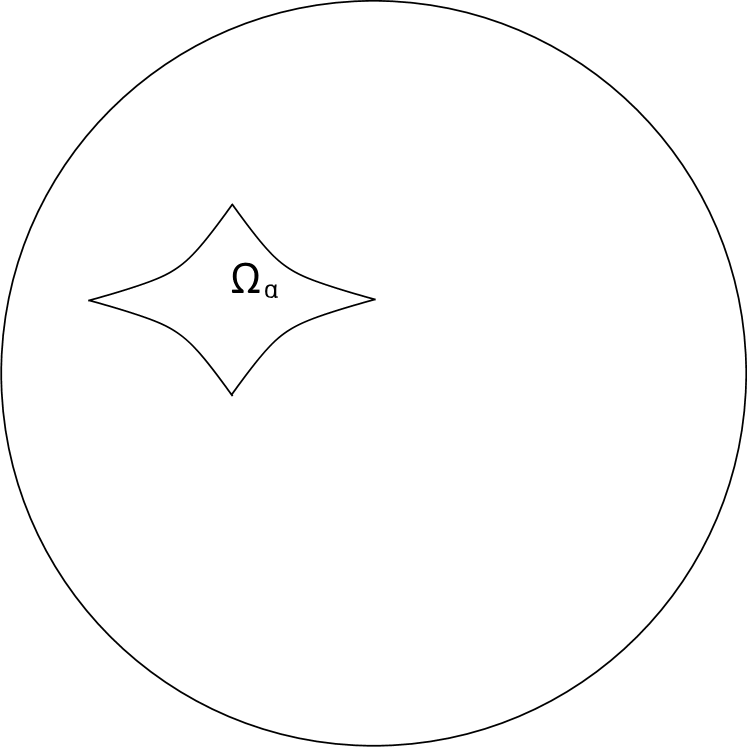
Figure 5: An exact mathematical Stability Zone $\,\Omega_{\alpha}\,$ on the unit sphere $\,\mathbb{S}^{2}\,$, corresponding to a fixed triple $\,(M^{\alpha}_{1},M^{\alpha}_{2},M^{\alpha}_{3})\,$.

Let us say, however, that the full set of directions of $\,{\bf B}\,$, corresponding to the presence of the open trajectories on the Fermi surface, has in general more complicated structure. Thus, it was first pointed out in GurzhyKop that the boundaries of the regions on the angle diagram, corresponding to appearance of the open trajectories, should have in fact a singular structure, which is caused by the difference between periodic and non-periodic trajectories arising on the Fermi surface. Using general topological description of the stable open trajectories of system (I.1) it can be shown that a general Stability Zone $\,\Omega_{\alpha}\,$ on $\,\mathbb{S}^{2}\,$ has necessarily an everywhere dense “net” of directions $\,{\bf B}\,\in\,\Omega_{\alpha}\,$, where the stable open trajectories of system (I.1) are actually periodic (JETP2017 ). Moreover, this net should be in fact extended outside the Zone $\,\Omega_{\alpha}\,$, since the periodic open trajectories still exist on its segments near the boundary of $\,\Omega_{\alpha}\,$. Let us note here, that according to our definition we don’t include the corresponding segments into the Zone $\,\Omega_{\alpha}\,$ since the corresponding trajectories are not stable anymore with respect to small rotations of $\,{\bf B}\,$. Besides that, the closed electron trajectories near the boundary of $\,\Omega_{\alpha}\,$ have in fact very specific form which makes them hardly distinguishable from the open trajectories from experimental point of view. As a result, the “experimentally observable Stability Zone” $\,{\hat{\Omega}}_{\alpha}\,$ is actually different from the exact mathematical Stability Zone (Fig. 6).

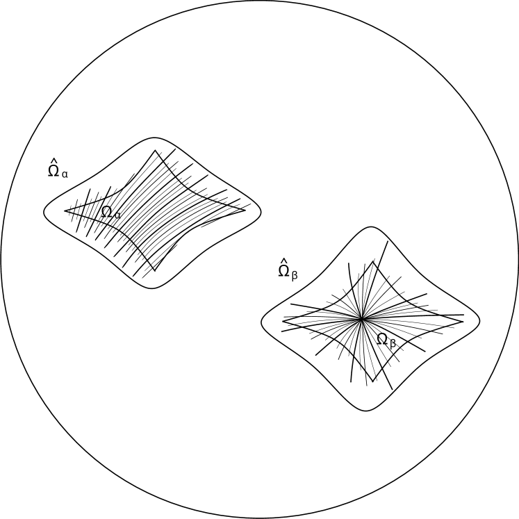
Figure 6: The “experimentally observable Stability Zones” with nets of special directions of $\,{\bf B}\,$ on the angle diagram.

Let us say also that due to the difference between the periodic and non-periodic trajectories the analytic dependence of the values $\,\sigma^{kl}({\bf B})\,$ both on the value and the direction of $\,{\bf B}\,$ is actually rather complicated both in the Zone $\,\Omega_{\alpha}\,$ and $\,{\hat{\Omega}}_{\alpha}\,$ (see JETP2017 ). As a result, the exact boundary of a mathematical Stability Zone $\,\Omega_{\alpha}\,$ is in fact unobservable in direct measurements of the values $\,\sigma^{kl}({\bf B})\,$ even for rather big values of $\,B\,$.

On the other hand, the exact form of the mathematical Stability Zones $\,\Omega_{\alpha}\,$ represents an important characteristic of the dispersion relation $\,\epsilon({\bf p})\,$ and can play rather important role in the reconstruction of the form of the Fermi surface from experimental data. In the present paper we will show that the oscillation phenomena in normal metals give in fact a convenient way to determine the boundary of the Zones $\,\Omega_{\alpha}\,$, which is based on the general topological structure of the “carriers of open trajectories” on the Fermi surface. In the next chapter we will give a description of the topological structure of a (complicated) Fermi surface in the presence of the stable open trajectories of system (I.1) and discuss special features of the oscillation phenomena on the surfaces of this kind.

II Special topological representation of a Fermi surface containing stable open trajectories and the oscillation phenomena in normal metals.

To describe the special topological representation of a complicated Fermi surface in presence of the stable open trajectories of system (I.1) let us introduce first a model Fermi surface, having the following form:

Consider a periodic set of parallel integral planes in ${\bf p}$ - space, connected by cylinders of finite heights (Fig. 7).

Figure 7: A model Fermi surface of genus 3 in ${\bf p}$ - space with stable open trajectories of system (I.1).

Let us divide all the planes into two different classes (I and II) - the odd-numbered planes and the even-numbered planes. Let us assume now that the planes of each class can be obtained from each other by a shift on some reciprocal lattice vector and represent the same object after the factorization over the reciprocal lattice.

In the same way, we assume that the cylinders are also divided into two classes which represent just two non-equivalent objects after the factorization.

We can say then that the periodic surface described above gives an example of a Fermi surface, which is represented as a pair of two parallel two-dimensional tori $\,\mathbb{T}^{2}\,\subset\,\mathbb{T}^{3}\,$ embedded in $\,\mathbb{T}^{3}\,$ and two cylinders of finite heights, connecting the tori $\,\mathbb{T}^{2}\,$.

Let us assume now that the axes of the cylinders are almost parallel in ${\bf p}$ - space and consider a magnetic field having a direction close to the direction of the axes of the cylinders. It is not difficult to see that if the direction of $\,{\bf B}\,$ is almost parallel to the cylinders then the cylinders consist mostly of closed trajectories of system (I.1), which cut our Fermi surface into separate parallel (deformed) planes. It can be also noted that the closed trajectories arising on the cylinders of different types also belong to different (the electron-type or the hole-type) types. The open trajectories of system (I.1) are given by the intersections of the planes, orthogonal to $\,{\bf B}\,$, with the periodically deformed integral planes in ${\bf p}$ - space and have the regular form shown at Fig. 4. The parts of the Fermi surface, consisting of closed trajectories, represent cylinders, restricted by singular trajectories, with heights, depending on the direction of $\,{\bf B}\,$. Thus, we have a Stability Zone around our initial direction of $\,{\bf B}\,$ with topological quantum numbers, defined by the homology class of the integral planes introduced above.

The boundary of the Stability Zone is defined by the condition that the height of the cylinders of one type becomes zero, such that the corresponding closed trajectories disappear on the Fermi surface (Fig. 8). As a result, the remaining closed trajectories can not cut the Fermi surface anymore into separate planes and we do not have stable open trajectories after the crossing the boundary of a Stability Zone. Thus, a Stability Zone represents in general a region with a piecewise smooth boundary in the space of directions of $\,{\bf B}\,$.

Figure 8: A very short cylinder of closed trajectories of one type for a direction of $\,{\bf B}\,$, close to the boundary of a Stability Zone.

Let us note, that we don’t claim here that the open trajectories of system (I.1) completely disappear outside the Stability Zone $\,\Omega\,$. Indeed, we can see that the remaining cylinders of closed trajectories now cut the Fermi surface into connected pairs of integral planes and the trajectories of system (I.1) still admit an effective description near the boundary of the Zone $\,\Omega\,$. It is not difficult to see, that the trajectories can now “jump” between two planes which gives a reconstruction of the open trajectories after the crossing of the boundary of the Zone $\,\Omega\,$. It can be seen also that all the open trajectories will transform into long closed trajectories if the intersection of the plane, orthogonal to $\,{\bf B}\,$, with the integral planes has an irrational direction in the ${\bf p}$ - space. At the same time, if the intersection of the plane, orthogonal to $\,{\bf B}\,$, and the integral planes has a rational direction, then we will have both the long closed trajectories and the open periodic trajectories near the boundary of the Zone $\,\Omega\,$. The open periodic trajectories, however, are not stable outside the Zone $\,\Omega\,$, so we should not include the corresponding set of directions of $\,{\bf B}\,$ in the mathematical Stability Zone. At the same time, this set belongs to the “experimentally observable Stability Zone”, which includes the mathematical Stability Zone as a subset. The analytical properties of the conductivity in the experimentally observable Stability Zone are in fact rather complicated (see JETP2017 ), which makes the experimental determination of the boundary of a mathematical Stability Zone a non-trivial problem.

The picture described above represents a Fermi surface of genus 3, embedded in the three-dimensional torus $\,\mathbb{T}^{3}\,$, and gives an example of complicated enough Fermi surface from topological point of view. In general, the topological representation of real complicated Fermi surface, carrying stable open trajectories of system (I.1), can differ from that described above in the following details:

1) The number of non-equivalent cylinders of closed trajectories can be bigger (or less) than 2;

2) There can be additional cylinders of closed trajectories on the integral planes, having a point as a base;

3) The number of non-equivalent parallel integral planes can be bigger than 2, being any even number (Fig. 9).

Let us say here that in the most general case we can also assume that parts of the Fermi surface consisting of closed trajectories and connecting carriers of open trajectories can have a composite structure and consist of several cylinders of closed trajectories inside some Stabilty Zone $\,\Omega_{\alpha}$. This possibility does not change the essence of our further considerations, and is extremely unlikely for real Fermi surfaces, so we will not dwell on it here. Thus, we can consider the described structure of the Fermi surface as the most common near the boundary of Stability Zones.

Figure 9: Topological representation of a Fermi surface of a very high genus carrying stable open trajectories of system (I.1).

The general statement formulated above represents a corollary of rather deep topological theorems, proved in the papers zorich1 ; dynn1 ; dynn3 . Let us say that the situation (3) can be observed actually only for surfaces of very high genus, so, for many real metals it actually does not arise. Let us note also, that the situation (3) can be considered also as an “overlapping” of two (or more) Stability Zones with the same topological quantum numbers. As was pointed out in JETP2017 , the analytical properties of conductivity are the most complicated in this situation, in particular, we should observe here more than one boundary of a Stability Zone (Fig. 10).

Figure 10: A complicated Stability Zone, representing an overlapping of two Zones with the same topological numbers.

In any situation the boundary of an exact mathematical Stability Zone is defined by vanishing of one of the cylinders of closed trajectories, so, as we will see below, the study of the oscillation phenomena gives in fact a convenient instrument to detect the boundary of a Stability Zone in experiment.

Let us say also here, that the picture described above represents a purely topological representation of a Fermi surface, carrying stable open trajectories (or, better to say, a topological representation of system (I.1) on the Fermi surface), and can be visually much more complicated due to possible complicated geometry of the objects, introduced above.

Below we will consider the oscillation phenomena in the picture described above and describe their special features near the boundary of a Stability Zone. Certainly, we will not give here a detailed theoretical exposition of the phenomena we are going to consider and give just a reference on their standard description (see e.g. etm ; Kittel ; Abrikosov ; Ziman ).

Let us start with the (classical) cyclotron resonance phenomenon, which can be described with the aid of the purely kinetic approach for the electron gas in normal metals. As it is well known, the cyclotron resonance phenomenon is connected with the oscillating dependence of the surface conductivity on the frequency of the alternating field in presence of a strong magnetic field $\,{\bf B}\,$. In the most common setting, the direction of $\,{\bf B}\,$ is assumed to be parallel to the metal surface and the alternating electric field can have different directions in the same plane. The oscillating behavior of the surface conductivity (in the situation of anomalous skin effect) is caused by the coincidence of the frequency $\,\Omega\,$ of the incident wave with the values $\,n\,\omega_{B}\,$, $\,n\in\mathbb{N}\,$, where $\,\omega_{B}\,=\,\omega_{B}(p_{z})\,$ is the cyclotron frequency, defined for every closed trajectory of system (I.1). In general, $\,\omega_{B}(p_{z})\,$ represents a complicated function of $\,p_{z}\,$ and the oscillating behavior of conductivity is determined in fact by the extremal values of $\,\omega_{B}(p_{z})\,$, satisfying the condition $\,d\omega_{B}/dp_{z}\,=\,0$.

In the geometric picture described above the closed trajectories are combined into cylinders connecting integral planes and we have the relation $\,\omega_{B}(p_{z})\,=\,0$ on the bases of the cylinders. As a result, the positive function $\,\omega_{B}(p_{z})\,$ should have at least one maximum at every cylinder, i.e. every cylinder of closed trajectories contains at least one extremal trajectory in the sense pointed above. Let us say, that theoretically we can have several maxima and minima of the function $\,\omega_{B}(p_{z})\,$ on a cylinder of closed trajectories, however, the situation of several critical points of $\,\omega_{B}(p_{z})\,$ on the same cylinder requires in fact rather complicated geometry of the dispersion relation. For simplicity, we will assume here that all the cylinders of closed trajectories contain just one extremal (maximal) value of $\,\omega_{B}(p_{z})\,$. As we will see, more complicated cases do not contain any fundamental differences from the simple case under consideration.

Let us make also another remark. For Fermi surfaces of not very high genus the boundary of a Stability Zone is defined by disappearance of just one cylinder of closed trajectories of system (I.1), which is invariant under the transformation $\,{\bf p}\rightarrow-{\bf p}\,$. In this case the extremal value of $\,\omega_{B}\,$ corresponds to the central cross-section of the cylinder by the plane orthogonal to $\,{\bf B}\,$ (Fig. 11). For more complicated Fermi surfaces (of a high genus) we can also have the situation when two non-equivalent cylinders, which transform into each other under the transformation $\,{\bf p}\rightarrow-{\bf p}\,$, disappear simultaneously on the boundary of a Stability Zone. Let us say, however, that this situation requires in fact a really complicated Fermi surface, so, in most of experiments we can actually assume the first case. Let us note also here, that the first situation has also the additional property

$$\langle v^{z}_{gr}\rangle_{tr}\,\,\,=\,\,\,0$$

on the extremal trajectories, which permits in fact not to impose too strict condition that $\,{\bf B}\,$ is parallel to the metal surface.

Figure 11: The extremal trajectory on a cylinder of closed trajectories of system (I.1).

Coming back to the cyclotron resonance phenomenon, we can see then that for the structure of the Fermi surface described above the oscillating conductivity behavior in high frequency electric fields should reveal a finite number of the main terms, representing the contribution of the extremal trajectories on the cylinders of closed trajectories and also of the endpoints of the special (degenerate) cylinders at Fig. 9. Let us also note here that the last contribution actually does not arise if the direction of $\,{\bf E}\,$ in the incident wave is orthogonal to our fixed direction of $\,{\bf B}\,$. Every main term is characterized by a periodic dependence on the frequency $\,\Omega\,$ (or on $\,1/B\,$) with its own period $\,T_{i}\,$. For directions of $\,{\bf B}\,$ lying inside a Stability Zone $\,\Omega_{\alpha}\,$ the periods $\,T_{i}({\bf B}/B)\,$ represent smooth functions of the direction of $\,{\bf B}\,$ and one of the periods $\,T_{i_{0}}\,$ becomes infinite at the boundary of the Stability Zone (Fig. 12). After crossing the boundary of a mathematical Stability Zone $\,\Omega_{\alpha}\,$ the corresponding contribution disappears completely, while all the other main contributions do not notably change (Fig. 13).

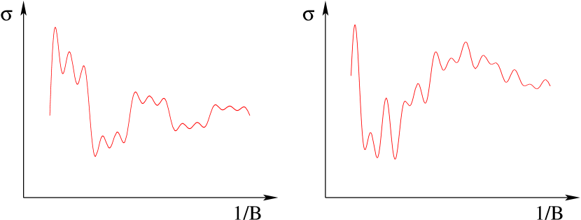
Figure 12: The increasing of the period of one of the main oscillating terms in the surface conductivity (real or imaginary part) near the boundary in a Stability Zone.

Figure 13: The disappearance of one of the main oscillating contributions in the surface conductivity after crossing the boundary of a Stability Zone.

Let us specially note here that both the vanishing of one of the main oscillating terms in the conductivity and increasing of its period $\,T_{i_{0}}\,$ have very sharp character near the boundary of a Stability Zone. Indeed, the main oscillating terms in conductivity are given by the contributions of very narrow “bands” of closed trajectories near the extremal trajectories, which do not change noticeably up to the boundary of the Zone $\,\Omega_{\alpha}\,$. In the same way, a noticeable increasing of the period $\,T_{i_{0}}\,$ is caused by a close approach of the singular trajectories to the extremal trajectory on a cylinder of closed trajectories (Fig. 8). It can be also shown, that this effect starts to manifest itself in a pretty narrow region near the boundary of $\,\Omega_{\alpha}\,$. As a result, the intermediate picture represented at Fig. 12 and Fig. 13 can in fact be practically unobservable in the experimental study of the cyclotron resonance phenomenon, such that we will most probably observe actually a more sharp transition (Fig. 14) after crossing the boundary of a Stability Zone.

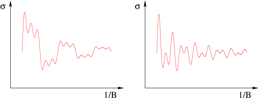
Figure 14: The schematic sharp change of the experimental picture of oscillations of the surface conductivity after crossing the boundary of a Stability Zone. It can be seen that the change in the oscillatory behavior is represented by the disappearance of one of the main oscillation terms from a finite sum of such terms.

We can see then that, despite the fact that the long closed trajectories arising outside a Stability Zone are hardly distinguishable from the open trajectories from experimental point of view, the cyclotron resonance phenomenon provides us a good tool for exact experimental determination of the boundary of a mathematical Stability Zone. Let us note also that the long closed trajectories arising near the boundary of a mathematical Stability Zone correspond to very large periods of electron motion along the orbit which can exceed the free electron motion time, so, they do not give in this case any visible contribution in the cyclotron resonance picture in experiment.

Let us discuss now briefly quantum oscillations phenomena in normal metals among which the oscillations of the magnetic susceptibility (De Haas - Van Alphen effect) and of the conductivity (Shubnikov - De Haas effect) with the value of $\,1/B\,$ are the most often mentioned.

The common reason for the quantum oscillation phenomena in normal metals is the quantization of the electron motion along the closed trajectories of system (I.1) in the plane orthogonal to $\,{\bf B}\,$. In the quasiclassical approximation we should put now that the closed trajectories of system (I.1) should be selected in accordance with the quantization rule

$$S(\epsilon,p_{z})\,\,\,=\,\,\,{2\pi e\hbar B\over c}\,\left(n+{1\over 2}\right)\,\,\,,\quad n\gg 1\,\,\,,$$

where $\,S(\epsilon,p_{z})\,$ is the area bounded by a closed trajectory of system (I.1) in the plane orthogonal to $\,{\bf B}\,$ in the ${\bf p}$ - space.

The quantum oscillations of physical quantities measured in metals are connected then with the crossing of the Fermi level by the corresponding quantized energy levels which defines us the period of the corresponding oscillations, brought by a fixed closed trajectory on the Fermi surface

$$\Delta\,{1\over B}\,\,\,=\,\,\,{2\pi e\hbar\over c\,S(\epsilon_{F},p_{z})}$$

Like in the case of the cyclotron resonance the main terms in the oscillating behavior are brought by the extremal closed trajectories, which are defined now by the condition $\,dS/dp_{z}\,=\,0\,$. As in the previous situation, we can expect here the presence of a finite number of trajectories of this kind on every cylinder, connecting integral planes, if $\,{\bf B}/B\,\in\,\Omega_{\alpha}\,$. Thus, the oscillating behavior of the physical quantities should be mainly represented here by several main oscillating terms, having different periods

$$\left(\Delta\,{1\over B}\right)_{i}\,\,\,=\,\,\,{2\pi e\hbar\over c\,S^{i}_{extr}}$$

in the variable $\,1/B\,$.

For not extremely complicated Fermi surfaces we can expect again that every cylinder of closed trajectories of system (I.1) contains just one trajectory corresponding to an extremal area in the ${\bf p}$ - space. Besides that, for the Fermi surfaces of not very high genus we can expect that every cylinder of closed trajectories is invariant under the transformation $\,{\bf p}\rightarrow-{\bf p}\,$, so, every extremal trajectory on this cylinder represents in fact its central cross-section by the plane orthogonal to $\,{\bf B}\,$. Let us say, however, that for very complicated Fermi surfaces the assumptions above are not necessarily fulfilled. In particular, in the situation when we have pairs of cylinders, transforming into each other under the transformation $\,{\bf p}\rightarrow-{\bf p}\,$, the extremal trajectories on them can be located near the bases of the cylinders. In general, the details pointed above do not change noticeably the scheme of using quantum oscillations phenomena for the determination of the exact boundary of Stability Zones for magneto-conductivity in normal metals.

Like in the case of the cyclotron resonance, we should observe here a “quick change” in the picture of oscillations of physical quantities after crossing the boundary of a Stability Zone, which is caused by the disappearance of one (or more) of the cylinders of closed trajectories of system (I.1). Also in this case the changes are sharply expressed at the boundary of $\,\Omega_{\alpha}\,$ since the corresponding main term in the oscillation picture is brought by an extremal trajectory, which remains almost the same up to the boundary of $\,\Omega_{\alpha}\,$ and disappears abruptly after crossing the boundary. The changes in the oscillation picture have the form, similar to that observed in the cyclotron resonance, showing the disappearance of one of the main oscillation terms (Fig. 14). Let us just note, that in this case we should not see at all an increasing of the corresponding period of oscillations near the boundary of $\,\Omega_{\alpha}\,$, since it is defined now by the area restricted by an extremal trajectory (and not cyclotron frequency), which does not change much near the boundary of a Stability Zone.

At last, let us make one more additional remark. As we saw above, the description of the quantum oscillations in normal metals is connected with the area bounded by an extremal trajectory in the plane orthogonal to $\,{\bf B}\,$. The extremal trajectories in the theory of the cyclotron resonance are defined by the extremal values of the cyclotron frequency, which is actually connected with the value $\,\partial S(\epsilon,p_{z})/\partial\epsilon\,$ according to the formulae

$$\omega_{B}\,\,\,=\,\,\,{eB\over m^{*}c}\quad,\quad\quad m^{*}\,\,\,=\,\,\,{1\over 2\pi}\,{\partial S(\epsilon,p_{z})\over\partial\epsilon}$$

At the same time, the value $\,\partial S(\epsilon,p_{z})/\partial\epsilon\,$ can be measured also in the experimental study of the quantum oscillations, using the investigation of their temperature dependence (etm ; Kittel ; Abrikosov ; Ziman ). We would like to point out here, that the values of $\,\partial S(\epsilon,p_{z})/\partial\epsilon\,$, measured by these two different ways should coincide in fact for $\,{\bf B}/B\,\in\,\Omega_{\alpha}\,$ for most of the real metals having not extremely complicated Fermi surfaces. The reason of this coincidence is given here by the fact, that both the cyclotron resonance phenomenon and the quantum oscillations phenomena are connected with the same extremal trajectories, given by the central cross-sections of the cylinders of closed trajectories in the topological representation of the Fermi surface according to Fig. 9. At the same time, for metals with extremely complicated Fermi surfaces, this circumstance may not take place in general, so, the values of $\,\partial S(\epsilon,p_{z})/\partial\epsilon\,$, measured in these two different ways, can be different, since they are connected now with different extremal trajectories of system (I.1). It’s not difficult to see, that our last remark has no direct relationship to the determination of the boundaries of the Stability Zones in metals, however, it can play a role in more detailed investigation of the oscillation phenomena for $\,{\bf B}/B\,\in\,\Omega_{\alpha}\,$.

III Conclusions.

We consider the problem of the exact determination of the boundary of a Stability Zone for magneto-conductivity of normal metals in the space of directions of $\,{\bf B}\,$. As can be shown, this problem is actually rather nontrivial from experimental point of view due to a substantial difference between the exact mathematical Stability Zones and the “experimentally observable Stability Zones” in the direct conductivity measurements. It can be shown, however, that the experimental detection of the exact boundary of a Stability Zone can be effectively implemented with the aid of the well-known oscillation phenomena such as the cyclotron resonance or quantum oscillations in normal metals. Thus, the experimental study of oscillation phenomena in sufficiently strong magnetic fields reveals a sharp change in the picture of the oscillatory behavior of physical quantities after crossing the boundary of the mathematical Stability Zone as functions of the value of $B$ for a given direction of the magnetic field. This abrupt change in the oscillatory behavior can be described in the general case as the disappearance of one of the principal terms from the total contribution, represented by a final sum of such terms (Fig. 14). So, a detailed study of the oscillatory behavior of physical quantities at different directions of ${\bf B}$ allows us actually to determine the precise boundaries of the mathematical Stability Zones for the magneto-conductivity of metals. The results of the paper are based on the topological description of the structure of the Fermi surface in the case of presence of stable open quasiclassical electron trajectories on it.

References

- (1) I.M.Lifshitz, M.Ya.Azbel, M.I.Kaganov. The Theory of Galvanomagnetic Effects in Metals., Sov. Phys. JETP 4:1 (1957), 41.
- (2) I.M. Lifshitz, V.G. Peschansky., Galvanomagnetic characteristics of metals with open Fermi surfaces., Sov. Phys. JETP 8:5 (1959), 875.
- (3) I.M. Lifshitz, V.G. Peschansky., Galvanomagnetic characteristics of metals with open Fermi surfaces. II., Sov. Phys. JETP 11:1 (1960), 137.
- (4) I.M. Lifshitz, M.I. Kaganov., Some problems of the electron theory of metals I. Classical and quantum mechanics of electrons in metals., Sov. Phys. Usp. 2:6 (1960), 831-835.
- (5) I.M. Lifshitz, M.I. Kaganov., Some problems of the electron theory of metals II. Statistical mechanics and thermodynamics of electrons in metals., Sov. Phys. Usp. 5:6 (1963), 878-907.
- (6) I.M. Lifshitz, M.I. Kaganov., Some problems of the electron theory of metals III. Kinetic properties of electrons in metals., Sov. Phys. Usp. 8:6 (1966), 805-851.
- (7) I.M. Lifshitz, M.Ya. Azbel, M.I. Kaganov., Electron Theory of Metals. Moscow, Nauka, 1971. Translated: New York: Consultants Bureau, 1973.
- (8) M.I. Kaganov, V.G. Peschansky., Galvano-magnetic phenomena today and forty years ago., Physics Reports 372 (2002), 445-487.
- (9) S.P. Novikov., The Hamiltonian formalism and a many-valued analogue of Morse theory., Russian Math. Surveys 37 (5) (1982), 1-56.
- (10) A.V. Zorich., A problem of Novikov on the semiclassical motion of an electron in a uniform almost rational magnetic field., Russian Math. Surveys 39 (5) (1984), 287-288.
- (11) I.A. Dynnikov., Proof of S.P. Novikov’s conjecture for the case of small perturbations of rational magnetic fields., Russian Math. Surveys 47 (3) (1992), 172-173.
- (12) S.P. Tsarev. Private communication. (1992-93).
- (13) I.A. Dynnikov., Proof S.P. Novikov’s conjecture on the semiclassical motion of an electron., Math. Notes 53:5 (1993), 495-501.
- (14) I.A. Dynnikov., Semiclassical motion of the electron. A proof of the Novikov conjecture in general position and counterexamples., Solitons, geometry, and topology: on the crossroad, Amer. Math. Soc. Transl. Ser. 2, 179, Amer. Math. Soc., Providence, RI, 1997, 45-73.
- (15) S.P. Novikov, A.Y. Maltsev., Topological quantum characteristics observed in the investigation of the conductivity in normal metals., JETP Letters 63 (10) (1996), 855-860.
- (16) I.A. Dynnikov., The geometry of stability regions in Novikov’s problem on the semiclassical motion of an electron., Russian Math. Surveys 54:1 (1999), 21-59.
- (17) S.P. Novikov, A.Y. Maltsev., Topological phenomena in normal metals., Physics-Uspekhi 41:3 (1998), 231-239.
- (18) A.Ya. Maltsev, S.P. Novikov., Quasiperiodic functions and Dynamical Systems in Quantum Solid State Physics., Bulletin of Braz. Math. Society, New Series 34:1 (2003), 171-210.
- (19) A.Ya. Maltsev, S.P. Novikov., Dynamical Systems, Topology and Conductivity in Normal Metals in strong magnetic fields., Journal of Statistical Physics 115:(1-2) (2004), 31-46.
- (20) R. De Leo., First-principles generation of stereographic maps for high-field magnetoresistance in normal metals: An application to Au and Ag., Physica B: Condensed Matter 362 (1–4) (2005), 62–75.
- (21) A.V. Zorich., Proc. “Geometric Study of Foliations”., (Tokyo, November 1993) / ed. T.Mizutani et al. Singapore: World Scientific, 479-498 (1994).
- (22) A.Y. Maltsev., Anomalous behavior of the electrical conductivity tensor in strong magnetic fields., JETP 85 (5) (1997), 934-942.
- (23) R. De Leo., Existence and measure of ergodic leaves in Novikov’s problem on the semiclassical motion of an electron., Russian Math. Surveys 55:1 (2000), 166-168.
- (24) R. De Leo., Characterization of the set of “ergodic directions” in Novikov’s problem of quasi-electron orbits in normal metals., Russian Math. Surveys 58:5 (2003), 1042-1043.
- (25) R. De Leo., Topology of plane sections of periodic polyhedra with an application to the Truncated Octahedron., Experimental Mathematics 15:1 (2006), 109-124.
- (26) R. De Leo, I.A. Dynnikov., An example of a fractal set of plane directions having chaotic intersections with a fixed 3-periodic surface., Russian Math. Surveys 62:5 (2007), 990–992.
- (27) R. De Leo, I.A. Dynnikov., Geometry of plane sections of the infinite regular skew polyhedron ., Geom. Dedicata 138:1 (2009), 51-67.
- (28) A. Skripchenko., Symmetric interval identification systems of order three., Discrete Contin. Dyn. Sys. 32:2 (2012), 643-656.
- (29) A. Skripchenko., On connectedness of chaotic sections of some 3-periodic surfaces., Ann. Glob. Anal. Geom. 43 (2013), 253-271.
- (30) I. Dynnikov, A. Skripchenko., On typical leaves of a measured foliated 2-complex of thin type., Topology, Geometry, Integrable Systems, and Mathematical Physics: Novikov’s Seminar 2012-2014, Advances in the Mathematical Sciences., Amer. Math. Soc. Transl. Ser. 2, 234, eds. V.M. Buchstaber, B.A. Dubrovin, I.M. Krichever, Amer. Math. Soc., Providence, RI, 2014, 173-200, arXiv: 1309.4884
- (31) R.N. Gurzhy, A.I Kopeliovich., Low-temperature electric conductivity of pure metals., In the book: Conductivity electrons., Red. M.I. Kaganov, V.S. Edelman., Moscow, Nauka, 1985 (in Russian).
- (32) A.Ya. Maltsev., On the Analytical Properties of the Magneto-Conductivity in the Case of Presence of Stable Open Electron Trajectories on a Complex Fermi Surface., Journal of Experimental and Theoretical Physics 124 (5) (2017), 805-831.
- (33) C. Kittel., Quantum Theory of Solids., Wiley, 1963.
- (34) A.A. Abrikosov., Fundamentals of the Theory of Metals., Elsevier Science & Technology, Oxford, United Kingdom, 1988.
- (35) J.M. Ziman., Principles of the Theory of Solids., Cambridge University Press 1972.