Exact diagonalization of cubic lattice models in commensurate Abelian magnetic fluxes and translational invariant non-Abelian potentials

Abstract

We present a general analytical formalism to determine the energy spectrum of a quantum particle in a cubic lattice subject to translationally invariant commensurate magnetic fluxes and in the presence of a general space-independent non-Abelian gauge potential. We first review and analyze the case of purely Abelian potentials, showing also that the so-called Hasegawa gauge yields a decomposition of the Hamiltonian into sub-matrices having minimal dimension. Explicit expressions for such matrices are derived, also for general anisotropic fluxes. Later on, we show that the introduction of a translational invariant non-Abelian coupling for multi-component spinors does not affect the dimension of the minimal Hamiltonian blocks, nor the dimension of the magnetic Brillouin zone. General formulas are presented for the $U(2)$ case and explicit examples are investigated involving $\pi$ and $2\pi/3$ magnetic fluxes. Finally, we numerically study the effect of random flux perturbations.

1 Introduction

The study of the effects of a magnetic field on a quantum particle and on its energy spectrum is a subject of research as old as quantum mechanics, with a plethora of applications ranging from the Aharonov-Bohm effect [1] to spintronics [2] and the quantum Hall effect [3]. A special role in this field is certainly played by the study of properties of particles subject to the combined effect of a periodic potential and a magnetic field, starting from the classic papers on the energy spectrum of Bloch electrons in rational and irrational magnetic fields [4, 5]. The durable interest for the study of the interplay between the discreteness introduced by the lattice potential and the effects of the magnetic fields is motivated both by the physical relevance and by the mathematical beauty of these systems and their variants, including the relation with the one-dimensional Harper model [6, 7], incommensurability effects [5, 8] and topological invariants [9].

The possibility of controlling the intensity and the properties of the applied magnetic fields play a crucial role and provides an essential tool to explore a rich variety of phenomena, occurring already at the single particle level, as clear for the Hofstadter problem [5]. Since gauge potentials can be exploited to modify and control the particle dynamics, they also provide an instrument to break or create new symmetries and to engineer non-trivial band structures, as exemplified by the integer quantum Hall effect, obtained just from the application of the simplest gauge potential, a constant magnetic field. When the dynamics of the electrons or atoms is coupled to some inner degree of freedom, as in the case of the spin-orbit coupling, then the minimal coupling can be done with non-Abelian gauge potentials. The non-trivial combination of pseudospin degrees of freedom and a non-Abelian lattice dynamics is indeed crucial for the implementation of many important models discussed in the last decade, including topological insulators and superconductors [10, 11, 12].

Beside the successes in realizing such models in solid state devices, the recent experimental developments in the field of ultracold atomic gases [13, 14, 15] opened new scenarios to realize Abelian and non-Abelian gauge potentials in optical lattices, for instance imposing laser-assisted tunneling amplitudes to trapped atoms [15, 16] (see as well the recent review [17] in the book [18]). The possibility of implementing tunable gauge potentials became a paradigmatic example of the tools that can be exploited in the experimental design of novel quantum phases of matter and is providing a remarkable arena of challenging mathematical developments.

Such tools prompted a huge variety of theoretical investigations, aimed to propose new realizations of non-trivial phenomena and models, including the study of the physics of the Hofstadter butterfly [5, 19, 20], Weyl, Dirac and Majorana fermions [21, 22, 23, 24, 25], extra dimensions [26, 27, 28] and the implementation of states with non-Abelian excitations [29]. As an example of application of synthetic gauge potentials, relevant for the purposes of this paper, we observe that in two dimensions one can obtain Dirac cones in square lattices with a magnetic $\pi$-flux (half of the elementary flux) threading each plaquette [30, 31, 32, 33]. Similar properties may also be obtained in three dimensions: cubic lattices with synthetic $\pi$ fluxes in each plaquette still allow to obtain Weyl fermions [22, 34, 35, 36]. Moreover, artificial non-Abelian potentials may enable the possibility to explore ranges of Hamiltonian parameters, for instance for the spin-orbit couplings, that would be difficult to achieve in corresponding solid state devices. Further advantages offered by these setups are the possibility to control the contact interactions through Feshbach resonances and to tune independently the synthetic magnetic field and the Zeeman terms.

The goal of this work is to provide a unified formalism to determine the energy spectrum of a quantum particle on a cubic lattice subject to translational invariant commensurate magnetic fluxes and in the presence of a general non-Abelian gauge potential, also position-independent. The reasons for such a study are twofold: i) in most of the proposals and the experimental realizations listed above, the gauge potentials are translational invariant and, despite several interesting instances have been considered, we think that it is still useful a systematic study of non-Abelian gauge configurations in the simultaneous presence of an Abelian magnetic field. ii) the interplay of Abelian and non-Abelian gauge potentials poses in general fascinating mathematical questions. For instance, we show that the magnetic Brillouin zone defined in absence of the non-Abelian terms remains unaltered when a translational invariant one is added. We also show that for a commensurate Abelian potential the optimal gauge choice decomposing the Hamiltonian into matrices with minimal dimension is the so-called Hasegawa gauge [34].

After the general discussion about non-Abelian gauge potentials, we examine the case of $U(2)$ gauge potentials, which is relevant for most of the realizations/studies mentioned above. We observe in Section 4 that, while for an Abelian gauge configuration translational invariance is explicit and amounts to have a homogeneous magnetic field, in the presence of non-Abelian potentials a different gauge invariant definition of translational invariance is required. Even though the non-Abelian configurations we focus on transform under $U(2)$, from the discussions in the text it will be clear that most of our results are still valid also for translationally invariant gauge configurations related to larger non-Abelian groups.

The plan of the paper is the following. We recall in Section 2 the case of Abelian translational invariant configurations with commensurate flux $\Phi$, focusing on the definition and on the structure of the magnetic Brillouin zone (MBZ). For the sake to maintain the paper self-consistent, we discuss in detail the purely Abelian case, showing that the so-called Hasegawa gauge yields, for any commensurate magnetic flux, the minimal dimension of the Hamiltonian blocks in which the lattice Hamiltonian can be decomposed. For completeness, we also consider generally anisotropic hoppings in the three directions and anisotropic magnetic fluxes. In Section 3 we introduce generic $U(2)$ configurations, also anisotropic, and derive the corresponding lattice Hamiltonian. We also deal with the definition of the MBZ for non-Abelian configurations. We find, in particular, that spatially-independent non-Abelian gauge potentials do not affect the structure of the MBZ, which turns out to depend only on the Abelian potential. The Hamiltonian in the Hasegawa gauge is explicitly written. As expected, the $SU(2)$ non-Abelian potential modifies the energy spectrum, leading in general to a splitting of the Abelian bands. In Section 4 we investigate more formally the non-Abelian nature and the translational invariance of a given gauge potential, using the general properties of the Wilson loop. In Section 5 we perform a discussion of the single particle spectrum in the presence of both Abelian and non-Abelian isotropic potentials, the latter one mimicking a spin-orbit coupling, relevant in various proposals and experimental settings. In particular, we focus on the Abelian magnetic fluxes $\Phi=\pi,2\pi/3$, when the strength of the non-Abelian gauge coupling is continuously varied. Finally, in Section 6 we analyze the effects of small flux perturbations on the single particle spectrum. A mapping of these perturbed models to generalized Aubry-André models is also described. We conclude the paper with an outlook on possible future developments and applications of the present work.

2 Commensurate Abelian fluxes

The analysis of the physics of a particle in a three-dimensional lattice subject to magnetic fluxes has been a recurrent problem in the literature for many decades. Many authors addressed this problem adopting different approaches and focusing on several properties of this system, see, for example [33, 34, 35, 36, 37, 38, 39, 40]. In this Section we describe a suitable formalism for the analysis of such systems; we complete and extend the analysis in [34, 37] to pose the basis for the study of the non-Abelian gauge potentials in the following sections.

We consider, in particular, a tight-binding model on a cubic lattice with $N=L^{3}$ sites and lattice spacing $a$, the particles on the lattice being subject to an Abelian uniform and static magnetic field. In order to have on each plaquette (with area ${a}^{2}$) of the lattice a magnetic flux $\Phi={B}{a}^{2}$, isotropic in the three directions, we consider a magnetic field $\vec{B}=\Phi\,(1,1,1)$. In the next Subsection 2.1 we deal with the case of anisotropic fluxes. The presence of such fluxes is connected to a phase $e^{i\Phi}$ for the hopping around a single plaquette. In presence of many species we can extend the subsequent treatment and results, given the fact that the Abelian gauge potential does not mix the different species.

We write the commensurate magnetic flux as

$$\Phi=2\pi\frac{m}{n}\,,$$ (1)

with $m$ and $n$ red co-prime integers. The commensurability, reflected in the condition (1), allows the analytical solution of the single particle spectrum (when the periodic boundary conditions are imposed) under the condition that the lattice encloses overall an integer number of fluxes in each direction, i.e. $L$ should be an integer multiple of $n$. In contrast, in the incommensurate case the spectrum can be reliably studied by rather heavy numerical computations on the real space tight-binding matrix [41].

The magnetic field $\vec{B}$ can be put in connection with the gauge potentials $A_{\mu}$, with $\mu=0,1,2,3$. Choosing the Weyl gauge $A_{0}(\vec{x})=0$, and following the usual formulation of a lattice theory in the presence of gauge potentials or fields (see for instance Ref. [42]), the real-space tight-binding Hamiltonian reads:

$$H=-\sum_{\vec{r}\,,\,\hat{j}}\,t_{\hat{j}}\,c^{\dagger}_{\vec{r}+\hat{j}}\,e^{i\phi_{\vec{r}+\hat{j},\vec{r}}}\,c_{\vec{r}}\,+\ \mathrm{H.c.}\,,$$ (2)

where the $t_{\hat{j}}$’s are the hopping amplitudes along the elementary displacements of the lattice, $\hat{j}=\hat{x},\hat{y},\hat{z}$. Periodic boundary conditions are assumed. This Hamiltonian constitutes a 3D extension of the Hofstadter model and its phases $\phi_{\vec{r}+\hat{j},\vec{r}}$ are given by

$$\phi_{\vec{r}+\hat{j},\vec{r}}=\int_{\vec{r}}^{\vec{r}+\hat{j}}\vec{A}_{\text{AB}}(\vec{x})\cdot\mathrm{d}\vec{x}\,,$$ (3)

where $\vec{r}=(x,y,z)$ denotes the position of lattice sites. The subscript in $\vec{A}_{\text{A}B}$ indicates that we are considering an Abelian gauge potential, and from Section 3 onward a non-Abelian gauge potential will be added to it. Here and in the following, we fix the lattice spacing $a=1$ for the sake of simplicity, even though when useful we will restore it. As anticipated above, the action of the magnetic field is to make a particle on the lattice acquire a phase at every hopping process, the sum of these phases along a closed loop amounting precisely to the magnetic flux threading the surface bounded by the loop, in agreement with Stokes theorem.

To study the effect of magnetic fluxes it is useful to recall the interplay between translational and gauge invariance in a system with a uniform magnetic field. We begin assuming a Hamiltonian in continuous space. Under this assumption, since the gauge potential is not constant like the related magnetic field, translational invariance implies that a translation of the coordinates by a vector $\vec{w}$ transforms the Hamiltonian as

$$\mathcal{T}^{\dagger}_{\vec{w}}(\vec{r})\,H(\vec{r}+\vec{w})\,\mathcal{T}_{\vec{w}}(\vec{r})=H(\vec{r})\,,$$ (4)

with $\mathcal{T}_{\vec{w}}(\vec{r})\in U(1)$ being a suitably chosen local gauge transformation which depends also on $\vec{w}$. This transformation acts on the Hamiltonian $H(\vec{r})$, linking the gauge potential at the point $\vec{r}$, $\vec{A}_{\text{A}B}(\vec{r})$, with the one at the translated point $\vec{r}+\vec{w}$, $\vec{A}_{\text{A}B}(\vec{r}+\vec{w})$:

$$\vec{A}_{\text{A}B}(\vec{r})\to\vec{A}_{\text{A}B}(\vec{r}+\vec{\omega})=\vec{A}_{\text{A}B}(\vec{r})-\,\vec{\nabla}\,\theta_{\vec{\omega}}(\vec{r})\,,$$ (5)

with $\theta_{\vec{\omega}}(\vec{r})$ a scalar function (see for instance Ref. [43]). To determine the phases $\theta_{\vec{w}}(\vec{r})$, we consider that the vector potential, in the case of a uniform magnetic field, is linear in the space coordinates. Therefore we can write it as a function of a $3\times 3$ matrix $Q$:

$$A_{{\text{A}B};j}(\vec{r})=Q_{ji}r_{i}\,,$$

where $A_{{\text{A}B};j}$ is the $j$-th component of $\vec{A}_{\text{A}B}$ ($j=x,y,z$). Under this assumption, the translation by $\vec{w}$ maps the vector potential into:

$$A_{{\text{A}B};j}(\vec{r})=Q_{ji}r_{i}\rightarrow A_{{\text{A}B};j}(\vec{r}+\vec{w})=Q_{ji}r_{i}+Q_{ji}w_{i}\,.$$ (6)

Therefore, to erase the contribution $Q_{ji}w_{i}$, based on Eq. (5), we must impose $\theta_{\vec{w}}(\vec{r})=r_{j}Q_{ji}w_{i}$. In this way, following the textbook approach [37], we can define a magnetic translation operator $T_{\vec{w}}$ as the composition of the space translation $\vec{\omega}$ with the gauge transformation $\mathcal{T}_{\vec{w}}(\vec{r})$, characterized by $\theta_{\vec{w}}(\vec{r})$:

$$T_{\vec{w}}\,\psi(\vec{r})=\mathcal{T}_{\vec{w}}(\vec{r})\,\psi(\vec{r}+\vec{w})=e^{-i\theta_{\vec{w}}(\vec{r})}\,\psi(\vec{r}+\vec{w})=\psi(\vec{r}).$$ (7)

The gauge redefinition of the wavefunction in Eq. (7) is an example of Berry phase.

Coming back to the tight-binding model for a translationally invariant system on a cubic lattice, the latter transformation translates into:

$$H=-\sum_{\vec{r}\,,\,\hat{j}}\,t_{\hat{j}}\,c^{\dagger}_{\vec{r}+\hat{j}}\,e^{i\theta_{\hat{j}}(\vec{r})}\,c_{\vec{r}}\,+\ \mathrm{H.c.}\,.$$ (8)

The related magnetic translation operators, $T_{\hat{x}},T_{\hat{y}}$, and $T_{\hat{z}}$, do not commute with each other in general. But, in the case of commensurate fluxes, it is possible to find multiples of the unit vectors such that:

$$\left[T_{a\hat{x}},T_{b\hat{y}}\right]=\left[T_{a\hat{x}},T_{c\hat{z}}\right]=\left[T_{b\hat{y}},T_{c\hat{z}}\right]=0\,.$$ (9)

A minimal triplet of integers $(a,b,c)$ of this kind defines a magnetic unit cell of volume $V_{uc}=abc$, playing a fundamental role in the definition of the MBZ. Indeed, the MBZ is defined by the reciprocal vectors (in quasi-momentum space) of three translations on the real lattice fulfilling the conditions in Eq. (9).

We point out that in a general gauge the phases $e^{i\theta_{\hat{j}}(\vec{r})}$ can be different from the ones defined in Eqs. (2) and (3), but the two sets are related by a gauge transformation as in Eq. (5). Moreover, Eq. (3) does not require translational invariance in general. Clearly, all the gauge-invariant quantities for the Hamiltonians in Eqs. (2) and (8) coincide, including the energies and the products of the phases around a chosen closed path (the Wilson loop). Finally, the two sets of phases exactly coincide in the specific gauge $\vec{A}(\vec{r})=\frac{1}{2}\,\vec{B}\times\vec{r}$ [37]. The concept of MBZ, just relying on translational invariance, can be defined for every gauge choice, starting from the phases defined as in Eqs. (2) and (3).

Due to the presence of the magnetic phases in Eq. (3), the sites of the lattice, which are equivalent for $\vec{B}=0$, are no longer equivalent. The lattice is then divided in a certain number of sublattices, and this division is gauge-dependent. This freedom may be exploited to individuate a gauge (or a set of gauges) giving rise to the smallest number of sublattices for the considered commensurate magnetic flux $\Phi=2\pi\frac{m}{n}$. It is clear that using the smallest number introduces a significant simplification in the computations.

This set of gauges can be identified as follows. When considering a magnetic field $\vec{B}$ which is constant in space, then each component of the vector potential $A_{i}(\vec{r})$ must be at most linear in the space coordinates $\{x,y,z\}$. In this way, concerning the definition of the hopping phases, the point $\{x,y,z\}$ is equivalent to the point $\{x+\mathsf{a}n,y+\mathsf{b}n,z+\mathsf{c}n\}$, $\mathsf{a,b,c}$ being integers, meaning that the two points belong to the same sublattice. Moreover, either a hopping phase is constant along a direction $\hat{i}$, or at least $n$ values for it are required.

Considering for a moment a two-dimensional square lattice, we conclude that the smallest number of its sublattices is $n$. This number is obtained, for instance, by setting to a constant ($0$ with no lack of generality) the magnetic phases along one direction and $\phi_{l}=2\pi\frac{m}{n}l$ ($l=0,\dots,n-1$) in the other one. A famous (and not unique) choice fulfilling these requirements is the Landau gauge $\vec{A}_{\mathrm{L}}=\Phi(0,x)$ [44], with $l=x\,\mathrm{mod}(n)$.

Let us focus now on a three-dimensional (3D) cubic lattice. In this case a single direction where the hopping phases are nonzero is clearly not sufficient, since the plaquette orthogonal to this direction would have $\Phi=0$. Then, the best one can do is to keep $\phi_{l}=2\pi\frac{m}{n}l$ along only a direction and set $\tilde{\phi}_{l}=f_{l}(\phi_{l})$ along another (with $f_{l}$ functions to be defined). In this way the number of sublattices still remains $n$. Finally, the linear dependence of $A_{i}(\vec{r})$ on $\{x,y,z\}$ and the requirement of constant flux on all the plaquettes implies $\tilde{\phi}_{l}=\phi_{(n-l)}\,\mathrm{mod}(2\pi)$. We conclude that the minimal number of sublattices is again $n$.

A gauge fulfilling the previous requirements and giving $n$ as dimension of the minimal Hamiltonian blocks is

$$\vec{A}_{\text{AB}}(\vec{r})=\frac{2\pi m}{n}\,(0,x-y,y-x)\,$$ (10)

(${x,y,z}$ can of course be permuted). The gauge (10), introduced by Hasegawa [34], can be seen as a three-dimensional extension of the Landau gauge in two dimensions, and it reduces (up to a gauge redefinition) to the Landau gauge itself for $t_{\hat{z}}\to 0$. In particular, this gauge is known to simplify the three-dimensional model by reducing it to an effective one-dimensional problem in momentum space [38]; this can be understood by observing that the explicit dependence on the position is a function of $x-y$ only, therefore there are two directions along which the momentum is conserved.

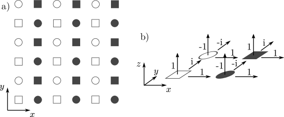
Figure 1: a) Division of the lattice in sub-sublattices for the case $\frac{m}{n}=\frac{1}{2}$ in the plane $(\hat{x},\hat{y})$. The $n=2$ different sublattices characterized by the sets of hopping phases in Eqs. (12,13) are denoted by circles and squares. For each sublattice it is convenient to define $n=2$ sub-sublattices which are represented as filled or empty symbols, respectively. b) The tunneling phases for $\frac{m}{n}=\frac{1}{2}$ are depicted.

Using the choice (10), the Hamiltonian (2) is rewritten in the form

$$H=-\sum_{\vec{r}}\left[t_{\hat{x}}\,c^{\dagger}_{\vec{r}+\hat{x}}\,c_{\vec{r}}+t_{\hat{y}}\,U_{\hat{y}}(x,y)\,c^{\dagger}_{\vec{r}+\hat{y}}c_{\vec{r}}+t_{\hat{z}}\,U_{\hat{z}}(x,y)\,c^{\dagger}_{\vec{r}+\hat{z}}c_{\vec{r}}\right]+\,\mathrm{h.c.}\,,$$ (11)

where $U_{\hat{j}}(x,y)=e^{i\phi_{\vec{r}+\hat{j},\vec{r}}}$. One finds $U_{\hat{x}}=1$ and the following expressions for $U_{\hat{y}}$, $U_{\hat{z}}$:

$$U_{\hat{y}}(x,y)=\exp\left[{i\,2\pi\,\Big{(}x-y-\frac{1}{2}\Big{)}\,\frac{m}{n}}\right]\,,$$ (12)

$$U_{\hat{z}}(x,y)=\exp\left[{-i\,2\pi\,\Big{(}x-y\Big{)}\,\frac{m}{n}}\right]\,.$$ (13)

Notice that in our discussion we may set $\frac{m}{n}<1$, since the spectrum is invariant for $\frac{m}{n}\to M-\frac{m}{n}$, with $M$ integer. We also observe that the $z$ coordinate is not present in Eq. (10), so that the eigenfunctions can be written as $\psi(x,y,z)=e^{ik_{z}z}\,u(x,y)$, with a dimensional reduction similar to the one occurring in two dimensions and giving rise to the Harper equation [5].

The Hamiltonian (11) satisfies Eq. (4) and is translationally invariant. We stress that the property in Eq. (4) is a physical property of the system which is reflected in all the gauge-invariant observables, as for example, in the Wilson loops evaluated on closed paths along the lattice. Furthermore, the Hamiltonian (11) is also periodic (with period $n$) along the $\hat{x}$ and $\hat{y}$ directions, so that the wavefunctions $u(x,y)$ have the same periodicity.

Therefore it is possible to build a magnetic unit cell, defined by the elementary translations leading from a site to equivalent ones in the three lattice directions, such that it is enlarged $n$ times along both these directions, thus including $n^{2}$ sites.

Consequently, the magnetic Brillouin zone (MBZ) is defined in momentum space as

$$[-\frac{\pi}{n},\frac{\pi}{n})\times[-\frac{\pi}{n},\frac{\pi}{n})\times[-\pi,\pi]\,.$$ (14)

It is clear, however, that other permutations of the factors $\frac{1}{n}$ between space directions amount to a gauge redefinition of $\vec{A}(\vec{r})$, leaving the energy spectrum unaltered. For periodic boundary condition and with the choice (14) there are ${N}/{n^{2}}$ allowed momenta $\vec{k}$. Setting $\vec{k}=(k_{x},k_{y},k_{z})$ with $k_{x},k_{y}\in[-\frac{\pi}{n},\frac{\pi}{n})$, and $k_{z}\in[-\pi,\pi)$, the components of $\vec{k}$ can be written as $k_{x}=\frac{2\pi}{L}\,{\cal N}_{x}$, $k_{y}=\frac{2\pi}{L}\,{\cal N}_{y}$ and $k_{z}=\frac{2\pi}{L}\,{\cal N}_{z}$, with ${\cal N}_{x,y}=0,\dots,\frac{L}{n}-1$ and ${\cal N}_{z}=0,\dots,L-1$, (similar expressions can be written if $N=L_{x}L_{y}L_{z}$ with $L_{j}$ the number of sites in the $\hat{j}$-direction).

To find the $N$ eigenvalues of the Hamiltonian  (11) on the considered cubic lattice with $N$ sites, one may exploit the division in sublattices just discussed. In particular we follow the approach in [37] to show that in the previously define MBZ, each eigenstate is $n-$fold degenerate. This is consistent with having $n$ bands, one for each sublattice, which are $n-$fold degenerate and include $N/n^{2}$ momenta.

Using the Hasegawa gauge (10), the cubic lattice can be divided in $n$ sublattices, which we label by $s=(x-y)\,\mathrm{mod}(n)$. One then gets

$$H=-\sum_{\hat{j}}t_{\hat{j}}\sum_{s}e^{i\phi_{s,\hat{j}}}\sum_{\vec{r}_{s}}\,c^{\dagger}_{\vec{r}_{s}+\hat{j}}\,c_{\vec{r}_{s}}\,+\mathrm{H.c.}\,,$$ (15)

where $s$ labels the different sublattices and $\vec{r}_{s}$ labels the sites of the $s$-th sublattice.

As a consequence, we expect $n$ sets of $\frac{N}{n}$ inequivalent energy eigenstates [37], forming in general $n$ subbands in the MBZ. Any sublattice, however, is further divided in $n$ sub-sublattices differing by a translation $\pm(\hat{x}+\hat{y})$, which leaves invariant the potential (10). Therefore, any set of eigenstates is again partitioned in $n$ equivalent and degenerate sub-sets, and each one of these has $\frac{N}{n^{2}}$ elements. These elements are labelled by the $\frac{N}{n^{2}}$ MBZ momenta according the previous description, with the second partition leading to an $n$-fold degeneracy of each subband.

In other words, with $\vec{k}$ belonging to the MBZ (14) one has $N/n^{2}$ possible values of $\vec{k}$, while the tight-binding Hamiltonian (2) has $N$ eigenvalues. For each of the $N/n^{2}$ values of $\vec{k}$ one has to diagonalize a $n\times n$ matrix, obtaining $N/n$ eigenvalues. Since each of them has a degeneracy $n$, we get the desired $N$ values for the eigenvalues of the Hamiltonian (2). In Fig. 1 we pictorially represent the division in sublattices and sub-sublattices for the case $\frac{m}{n}=\frac{1}{2}$.

We define

$$c_{\vec{r}_{s}}=\frac{1}{\sqrt{N/n^{2}}}\,\sum_{\vec{k}}\,c_{s}(\vec{k})\,e^{i\vec{k}\cdot\vec{r}_{s}}$$

with $\vec{r}_{s}$ indexing the $\frac{N}{n^{2}}$ sites of the sub-sublattice of the sublattice $s$. The Hamiltonian (15) is then written as

$$H=-\sum_{\vec{k}}\sum_{\hat{j}}t_{\hat{j}}\sum_{s}e^{iA_{s,\hat{j}}}\,e^{-i\vec{k}\cdot\hat{j}}\,c^{\dagger}_{s^{\prime}}(\vec{k})\,c_{s}(\vec{k})\,+\mathrm{H.c.}\,.$$ (16)

In Eq. (16) we used $s^{\prime}\equiv s+\hat{j}$ to label the sublattice in which the particle moves into after the hopping; in particular $s$ and $s^{\prime}$ coincide for the motion along $\hat{z}$ whereas they do not for the tunneling along $\hat{x}$ and $\hat{y}$, due to the potential (10).

The Hamiltonian (16) can be written in matrix notation as

$$H=-\sum_{\vec{k}}\sum_{\hat{j}}t_{\hat{j}}\sum_{s}\,c^{\dagger}_{s^{\prime}}(\vec{k})\Big{(}T_{\hat{j}}^{\mathrm{AB}}\Big{)}_{s^{\prime},s}\,e^{-i\vec{k}\cdot\hat{j}}\,c_{s}(\vec{k})\,+\,\mathrm{H.c.}\,.$$ (17)

The $T_{\hat{j}}^{\mathrm{AB}}$ are $n\times n$ matrices in the sublattice basis. Using the notation of Ref. [17], they read:

$$T_{\hat{x}}^{\mathrm{AB}} =\begin{pmatrix}0&1&0&0\\ 0&0&\ddots&0\\ 0&\ldots&0&1\\ 1&0&\ldots&0\end{pmatrix}\,,$$

$$T_{\hat{y}}^{\mathrm{AB}} =e^{-i\pi\frac{m}{n}}\,\begin{pmatrix}0&\ldots&0&\varphi_{0}\\ \varphi_{1}&0&\ldots&0\\ 0&\ddots&0&0\\ 0&0&\varphi_{n-1}&0\end{pmatrix}\,,$$

$$T_{\hat{z}}^{\mathrm{AB}} =\begin{pmatrix}\varphi_{0}&0&\ldots&0\\ 0&\varphi_{n-1}&0&0\\ 0&0&\ddots&0\\ 0&\ldots&0&\varphi_{1}\end{pmatrix}\,,$$ (18)

where we introduced the notation $\varphi_{l}\equiv e^{i2\pi\frac{m}{n}l}\,,\,l=0,\dots,n-1$. We observe that the $n^{\rm th}$ power of the matrices $T_{\hat{x},\hat{y},\hat{z}}^{\mathrm{AB}}$ gives the identity matrix. It is important to observe that when $\frac{m}{n}\neq\frac{1}{2}$, the matrices $T_{\hat{x},\hat{y},\hat{z}}^{\mathrm{AB}}$ are not invariant by the conjugate operation, expressing the fact that there is breaking of time-reversal symmetry. Finally, we observe that the previous results also apply in the presence of $p$ species (labeled by the index $\alpha=1,\dots,p$) subject to the Abelian gauge potential in Eq. (10). The Hamiltonian can be again written as $H=\sum_{\vec{k}}H(\vec{k})$ with

$$H({\vec{k}})=-\sum_{\hat{j}}t_{\hat{j}}\sum_{s}\,c^{\dagger}_{s^{\prime}=s+\hat{j},\alpha^{\prime}}(\vec{k})\left(T_{\hat{j}}^{\mathrm{AB}}\otimes{\bf 1}_{p\times p}\right)_{s^{\prime},\alpha^{\prime},s,\alpha}\,e^{-i\vec{k}\cdot\vec{j}}\,c_{s,\alpha}(\vec{k})\,+\,\mathrm{H.c.}\,.$$ (19)

In conclusion, the diagonalization of a $N\times N$ matrix is reduced for a single degree of freedom to the diagonalization of a $n\times n$ one. Moreover, the spectrum is predicted to divide in $n$ subbands generally having different energies. This fact provides a decomposition of the original Hamiltonian into matrices having the minimal dimension. In the particular case $\Phi=\pi$, two sub-bands are obtained, touching at Weyl cones as discussed in Refs. [22, 45, 46], providing the direct three-dimensional generalization of the square lattice model with $\pi$-fluxes discussed.

2.1 Anisotropic Abelian lattice fluxes

In the previous analysis we considered generally different hoppings $t_{\hat{j}}$ in the different space directions, but the same flux for the three orientations of the plaquettes. The latter condition can be relaxed to the case of anisotropic Abelian lattice fluxes. For the general magnetic field

$$\vec{B}=2\,\pi\,\Big{(}\frac{m_{x}}{n_{x}},\frac{m_{y}}{n_{y}},\frac{m_{z}}{n_{z}}\Big{)}\,,$$ (20)

it is convenient to choose the gauge potential

$$\vec{A}_{\text{AB}}(\vec{r})=2\pi\,\Bigg{(}\Big{(}\frac{m_{y}}{n_{y}}-\frac{m_{x}}{n_{x}}\Big{)}\,(z-x),\frac{m_{z}}{n_{z}}\,(x-y),\frac{m_{x}}{n_{x}}\,(y-x)\Bigg{)}\,.$$ (21)

One has then for the magnetic phases

$$\phi_{\vec{r}+\hat{j},\vec{r}}=2\pi\,\Bigg{(}\Big{(}\frac{m_{y}}{n_{y}}-\frac{m_{x}}{n_{x}}\Big{)}\,\Big{(}z-x-\frac{1}{2}\Big{)},\frac{m_{z}}{n_{z}}\,\Big{(}x-y-\frac{1}{2}\Big{)},\frac{m_{x}}{n_{x}}\,(y-x)\Bigg{)}\,.$$ (22)

The important comment we would like to stress is that the gauge (21) again guarantees that there is the minimum number of (gauge-dependent) sublattices. In particular, we obtain $n_{s}$ inequivalent sublattices, with

$$n_{s}=\mathrm{l.c.m.}(n_{x},n_{y},n_{z})\,.$$ (23)

Also in the considered case of anisotropic Abelian gauge potentials, each sublattice can be further divided in equivalent sub-sublattices following the same procedure detailed in the previous Section (se also [18]). Each inequivalent sublattice divides in $n_{d}$ equivalent sub-sublattices, with

$$n_{d}=\mathrm{min}\Big{(}\mathrm{l.c.m.}(n_{x},n_{y})\,,\,\mathrm{l.c.m.}(n_{x},n_{z})\Big{)}\,.$$ (24)

There are $\frac{N}{n_{s}\,n_{d}}$ quasi-momenta defining each subband, with $k_{x}=\frac{2\pi}{L}\,{\cal N}_{x}$, $k_{y}=\frac{2\pi}{L}\,{\cal N}_{y}$, and $k_{z}=\frac{2\pi}{L}\,{\cal N}_{z}$, with ${\cal N}_{x}=0,\dots,\frac{L}{n_{s}}-1$, ${\cal N}_{y}=0,\dots,\frac{L}{n_{d}}-1$, and ${\cal N}_{z}=0,\dots,L-1$. The Hamiltonian (2) is then finally rewritten in the above defined MBZ and in the basis of the $n_{s}$ sublattices as in Eq. (17), and three $n_{s}\times n_{s}$ matrices are derived similarly to what has beed done in the previous Section for the three matrices $T_{\hat{j}}^{\mathrm{AB}}$ in Eq. (18). Similar results can be obtained using a different optimal gauge choice through the mapping onto a one-dimensional model in momentum space [38].

3 Translationally invariant non-Abelian gauge potentials

We generalize here the Abelian models described in the previous Section, considering two species of particles hopping on the cubic lattice. For convenience, we label the effective spin degrees of freedom as ${\uparrow}$ and ${\downarrow}$. In current ultracold atoms experiments, the two species can be obtained, for instance, by populating selectively two different hyperfine levels of a certain atom [14]. In addition to the commensurate magnetic field $\vec{B}$ with plaquette flux $\Phi=2\pi\frac{m}{n}$, we impose that these particles are subject to the effect of a non-Abelian, time-independent, translationally invariant $SU(2)$ gauge potential. Such a potential plays the role of a generalized spin-orbit coupling and it links in non-trivial ways the dynamics of the atoms with their spin, mixing the spin species. From the point of view of the gauge group of the system, the models analyzed possess a gauge symmetry $U(2)\equiv\frac{SU(2)\times U(1)}{Z_{2}}$, which includes also the Abelian $U(1)$ symmetry group related with the conservation of the total number of particles $N_{\rm tot}=N_{\uparrow}+N_{\downarrow}$ [47].

The generating algebra of $U(2)$ is $u(2)=su(2)\oplus u(1)$. In the basis $({\uparrow},{\downarrow})$ the corresponding matrix representation can be taken as $\{{\vec{\sigma},{\bf 1}}\}$, $\vec{\sigma}$ being the Pauli matrices. We define a generic $U(2)$ vector potential which is composed by the isotropic configuration of Abelian fluxes that we considered in the previous Section, combined with a translationally invariant non-Abelian $SU(2)$ contribution:

$$\vec{A}(\vec{r})=\vec{A}_{\text{AB}}(\vec{r})+\vec{A}_{\text{NAB}}\,.$$ (25)

The Abelian gauge potential is written as in the previous Section in the Hasegawa gauge:

$$\vec{A}_{\text{AB}}(\vec{r})=2\pi\,\frac{m}{n}(0,x-y,y-x){\bf 1}\,,$$ (26)

where ${\bf 1}$ is the $2\times 2$ identity matrix. The non-Abelian gauge potential we consider reads

$$\vec{A}_{\text{NAB}}(\vec{r})=(\vec{f}_{x}\cdot\vec{\sigma},\vec{f}_{y}\cdot\vec{\sigma},\vec{f}_{z}\cdot\vec{\sigma})\,,$$ (27)

where the vectors $\vec{f}_{x},\vec{f}_{y},\vec{f}_{z}$ do not depend explicitly on position. An additional term $(d_{x},d_{y},d_{z})\,{\bf 1}$ in Eq. (27) can be erased by a gauge transformation.

The resulting tight-binding Hamiltonian, generalizing Eq. (15), reads

$$H=-\sum_{\vec{r},\alpha,\alpha^{\prime}}\left[t_{\hat{x}}\,U_{x,\alpha\alpha^{\prime}}(\vec{r})\,c^{\dagger}_{\vec{r}+\hat{x},\alpha^{\prime}}\,c_{\vec{r},\alpha}+t_{\hat{y}}\,U_{y,\alpha\alpha^{\prime}}(\vec{r})\,c^{\dagger}_{\vec{r}+\hat{y},\alpha^{\prime}}c_{\vec{r},\alpha}+\right.\\ \left.+t_{\hat{z}}\,U_{z,\alpha\alpha^{\prime}}(\vec{r})\,c^{\dagger}_{\vec{r}+\hat{z},\alpha^{\prime}}c_{\vec{r},\alpha}\right]+\,\mathrm{H.c.}\,,$$ (28)

where $\alpha$ and $\alpha^{\prime}$ label the spin indices. In the considered case $U_{\hat{x}}\,,\,U_{\hat{y}}\,,U_{\hat{z}}$ are now matrices. $U_{\hat{x}}$ does not depend on the position, unlike $U_{\hat{y}}\,,U_{\hat{z}}$: we find

$$U_{\hat{x}}=\exp\left({i\int_{x,y,z}^{x+1,y,z}A_{x}}\,\mathrm{d}x\right)=\exp\left({i\,\vec{f}_{x}\cdot\vec{\sigma}}\right)\,,$$ (29)

$$U_{\hat{y}}(x,y)=\exp\left({i\int_{x,y,z}^{x,y+1,z}A_{y}}\,\mathrm{d}y\right)=\exp\left[{i\,2\pi\,\Big{(}x-y-\frac{1}{2}\Big{)}\,\frac{m}{n}+i\,\vec{f}_{y}\cdot\vec{\sigma}}\right]\,,$$ (30)

$$U_{\hat{z}}(x,y)=\exp\left({i\int_{x,y,z}^{x,y,z+1}A_{z}}\,\mathrm{d}z\right)=\exp\left[{-i\,2\pi\,\Big{(}x-y\Big{)}\,\frac{m}{n}+i\,\vec{f}_{z}\cdot\vec{\sigma}}\right]\,$$ (31)

(remember that $a\equiv 1$). The Hamiltonian in Eq. (28) with the gauge potential in Eq. (27) is again translationally invariant because it fulfills Eq. (4). One can easily see that, since the non-Abelian term is position-independent, the translational invariance of the model is defined exactly as in the Abelian case and it is a gauge-invariant feature. In the same way, the potential in Eq. (27) is genuinely non-Abelian, since it is not gauge equivalent to any other Abelian gauge potential. These general properties of the potential $\vec{A}$ will be discussed in more detail in the next section.

The gauge transformations of the system in Eq. (28), with gauge potential given by Eqs. (25)–(27), are defined by the following unitary operators $\mathcal{U}$:

$$c_{\vec{r},\alpha}\to\mathcal{U}(\vec{r})_{\alpha,\alpha^{\prime}}c_{\vec{r},\alpha^{\prime}}\,,\quad\vec{A}(\vec{r})_{\alpha,\beta}\to\mathcal{U}(\vec{r})_{\alpha,\alpha^{\prime}}\vec{A}(\vec{r})_{\alpha^{\prime},\beta^{\prime}}\mathcal{U}^{\dagger}(\vec{r})_{\beta^{\prime},\beta}+i\,\mathcal{U}^{\dagger}(\vec{r})_{\alpha,\gamma}\left(\vec{\nabla}\mathcal{U}(\vec{r})\right)_{\gamma,\beta}\,,$$ (32)

where we sum over repeated indices. The previous transformations imply that the tunneling operators undergo the following transformation:

$$U_{\hat{j}}(\vec{r})\to\mathcal{U}(\vec{r}+\hat{j})U_{\hat{j}}(\vec{r})\mathcal{U}^{\dagger}(\vec{r})\,.$$ (33)

Any local gauge transformation $\mathcal{U}$ leaves the Hamiltonian in Eq. (28) invariant.

The wavefunctions of the same Hamiltonian can be again written as

$$\psi(x,y,z)=e^{ik_{z}z}\,u(x,y)\,,$$ (34)

where $u(x,y)$ is a periodic function with period $n$. For the same reason, the cubic lattice still divides in $n$ sublattices. The momentum-space Hamiltonian now takes the form

$$H=\sum_{\vec{k}}H(\vec{k})$$ (35)

with

$$H(\vec{k})=-\sum_{\hat{j}}t_{\hat{j}}\sum_{s,\alpha,\alpha^{\prime}}\,c^{\dagger}_{s^{\prime}\equiv s+\hat{j},\alpha^{\prime}}(\vec{k})\left(T_{\hat{j}}^{\mathrm{AB}}\otimes e^{i\,\vec{f}_{j}\cdot\vec{\sigma}}\right)_{{s^{\prime}},\alpha^{\prime},s,\alpha}\,e^{-i\vec{k}\cdot\vec{j}}\,c_{s,\alpha}(\vec{k})+\,\mathrm{H.c.}\,,$$ (36)

where we used the same notation as in Eq. (19). For generic values of $\vec{f}_{x},\vec{f}_{y},\vec{f}_{z}$, the Hamiltonian in Eq. (36) has the same symmetries of the one in Eq. (17). As a consequence, its spectrum divides in $2n$ generally non-degenerate subbands. We finally notice that non-Abelian gauge potentials with $SU(2)$ group symmetry are the most general ones fully implementable on a cubic lattice, since $SU(2)$ has only three independent generators. Gauge potentials with larger symmetry groups require non-cubic, more involved three-dimensional lattices.

The counting of eigenvalues goes as follows: the tight-binding Hamiltonian (28), defined for $N$ sites and $S=2$ inner degrees of freedom, has $SN$ eigenvalues. The possible values of ${\vec{k}}$ in the MBZ (14) (unaltered by the presence of the non-Abelian terms) are $N/n^{2}$. For each of them one has to diagonalize a $Sn\times Sn$ matrix, for a total of $SN/n$ eigenvalues. Each of such eigenvalues has degeneracy $n$, giving the desired $SN$ eigenvalues. The same goes on for a Hamiltonian defined for general $S$ degrees of freedom (or components).

Eqs. (35) and (36) are the main result of the paper, since they show that in the presence of a commensurate Abelian gauge potential with flux $\Phi=2\pi\frac{m}{n}$ (with $m$ and $n$ integers) and of a general translational invariant non-Abelian gauge potential acting on a particle with two inner degrees of freedom, the diagonalization of the Hamiltonian can be reduced to the diagonalization of a $2n\times 2n$ matrix in the MBZ, with the MBZ unaltered by the non-Abelian terms. It is clear that if the particle has $S$ degrees of freedom, then the matrix to be diagonalized is $Sn\times Sn$. We finally observe that the previous treatment can be used for $t_{\hat{z}}\to 0$ to study the two-dimensional limit of the Hamiltonian in Eq. (36) with general non-Abelian gauge potentials.

In the following we give a couple of physically relevant applications of Eq. (36) in Sections 5 and 6, but before we present in Section 4 a general, more formal discussion of the properties of a non-Abelian gauge potential.

4 General properties of a non-Abelian gauge potential

In this section we review the rigorous definition of non-Abelianity of the gauge potential and we adopt it to study the effects of translational invariance in these systems. In particular, we show that the Brillouin zone of the 3D Hofstadter model is not affected by the introduction of a potential of the form $\vec{A}_{\rm NAB}$ in Eq. (27).

The non-Abelian nature of this $U(2)$ potential seems evident from the fact that $\vec{A}_{\mathrm{NAB}}$ presents, in general, non-commuting components in the three directions. This implies that also the tunneling operators $U_{\hat{j}}\left(\vec{r}\right)$ in the site $\vec{r}$ do not commute with each other. Neither $\vec{A}_{\mathrm{NAB}}$ nor the operators $U_{\hat{j}}$, though, are gauge-invariant objects, and, as a result, also the commutators $\left[{A}_{\rm{NAB},\hat{j}},{A}_{\rm{NAB},\hat{k}}\right]$ and $\left[U_{\hat{j}},U_{\hat{k}}\right]$ depend on the gauge choice. This means that, in principle, there are seemingly non-Abelian gauge configurations that can be mapped into a fully Abelian case with $\left[{A}_{\rm{NAB},\hat{j}},{A}_{\rm{NAB},\hat{k}}\right]=\left[U_{\hat{j}},U_{\hat{k}}\right]=0$ with a suitable position-dependent gauge transformation in $U(2)$. The underlying model would thus be Abelian despite the conditions $\left[{A}_{\rm{NAB},\hat{j}},{A}_{\rm{NAB},\hat{k}}\right]\neq 0$ and $\left[U_{\hat{j}},U_{\hat{k}}\right]\neq 0$ in the initial gauge choice. Therefore one needs a criterion to define a genuinely non-Abelian potential which cannot be mapped into an Abelian model with any gauge transformation.

For this purpose, it is useful to consider first the Wilson operator around a closed and oriented path $\mathcal{C}$:

$$W(\mathcal{C},\vec{r})=\mathbb{P}\,e^{i\oint_{\mathcal{C},\vec{r}}\vec{A}(\vec{r^{\prime}})\cdot d\vec{r^{\prime}}}\,,$$ (37)

where $\mathbb{P}$ denotes path ordering, required since the gauge potential matrices calculated at different points do not commute in general in the non-Abelian case, and $\vec{r}$ is the position of the initial and final site of $\mathcal{C}$, arbitrarily chosen. While for an Abelian gauge configuration the operator $W(\mathcal{C})$ is gauge-invariant, related by the Stokes theorem to the magnetic flux on $\mathcal{C}$, and it is independent on $\vec{r}$, this is not so for a non-Abelian gauge configurations. Indeed in the latter case $W(\mathcal{C},\vec{r})$ transforms under the gauge group as [48]

$$W(\mathcal{C},\vec{r})\to\mathcal{U}^{\dagger}(\vec{r})\,W(\mathcal{C},\vec{r})\,\mathcal{U}(\vec{r})\,,$$ (38)

Despite this gauge dependence, though, Wilson loops provide a sufficient criterion to define the genuine non-Abelian nature of the potential [16]. We may refer to a gauge potential as genuinely non-Abelian if there exist at least two closed paths $\mathcal{C}_{1}$ and $\mathcal{C}_{2}$ on the lattice, originating from the same site $\vec{r}$, such that the operators $W(\mathcal{C}_{1},\vec{r})$ and $W(\mathcal{C}_{2},\vec{r})$ do not commute with each other:

$$\left[W(\mathcal{C}_{1},\vec{r}),W(\mathcal{C}_{2},\vec{r})\right]\neq 0\,.$$ (39)

Indeed, if (39) hold, then $W(\mathcal{C}_{1},\vec{r})$ and $W(\mathcal{C}_{2},\vec{r})$ cannot be put both in a diagonal form by the same gauge transformation $\mathcal{U}(\vec{r})$; therefore there exists no gauge choice in which the gauge potential can be written in a purely Abelian form. We stress however that the latter criterium, although satisfactory from a mathematical point of view, results practically useless operatively, since exploiting it for a general gauge configuration leads to an exponentially (with the lattice size) hard problem. Instead, a different criterium overpassing this limit is still missing in our knowledge.

In an explicitly translational invariant system, condition (39) can be simply verified for a single site, by looking at the minimal Wilson operators that describe the transport of an atom around a single lattice plaquette $\Box$; we define them as $W_{\hat{j}}(\Box)$, $\hat{j}$ labelling the orientation of the plaquette. The described situation holds for the potential in Eq. (27). It is not possible to simultaneously diagonalize the three the plaquette operators $W_{\hat{j}}(\Box)$ through a gauge transformation: even though one can always find a gauge in which one of then is diagonal (writable as a combination of the identity matrix and $\sigma_{z}$), In this case at least two closed lattice paths $\mathcal{C}_{1}$ and $\mathcal{C}_{2}$ exist, originating from the same site $\vec{r}$, such that (39) is fulfilled, showing the intrinsic non-Abelian character of the potential (27).

In the case of the potential (27), its translational invariance is obvious due to its independence on the space coordinates. In general, though, the definition of translation invariance in the non-Abelian case requires more care. Indeed the qualitative difference between the Abelian and non-Abelian case lies again in the gauge-dependent behavior of the Wilson loops in the second case, as outlined by Eq. (38).

For the Abelian potentials, a sufficient condition for translation invariance is that $W_{\hat{j}}(\Box)$ shall not depend on the initial and final site $\vec{r}$ of $\Box$, but only on the orientation of the plaquette, $\hat{j}$. In this case, by the Stokes theorem we have $W_{\hat{j}}(\Box)=e^{i\Phi_{\hat{j}}}$, where $\Phi_{\hat{j}}$ is a constant magnetic flux piercing each of the $\hat{j}$-oriented plaquettes.

For a non-Abelian gauge potential, instead, an explicit dependence of $W_{\hat{j}}(\Box)$ on the location $\vec{r}$ of $\Box$ does not necessarily imply the absence of translational invariance. A sufficient condition for translational invariance is indeed the existence of a gauge choice such that all the Wilson loops $W_{\hat{j}}(\Box)$ do not depend on $\vec{r}$. However, since the Wilson loops $W_{\hat{j}}(\Box)$ are not gauge invariant, but transform as in Eq. (38), even if they are position independent in a specific gauge, they can acquire a non-trivial space dependence after a generic local gauge transformation $\mathcal{U}(\vec{r})$.

In general, a Stokes theorem can be still formulated for $\mathrm{W}_{\hat{j}}(\Box)$ in the non-Abelian case [49], but the effective fluxes defined by it are not gauge invariant quantities. The physical origin of this fact is that, due to the non-linear nature of the non-Abelian gauge freedom (see for example [48]), the magnetic flux lines are themselves sources of flux.

Because of the transformation in Eq. (38), we are then led to conclude that the Wilson loop itself cannot be used any longer to probe translational invariance in the non-Abelian case. When we consider $U(\mathcal{N})$ gauge potentials, though, each Wilson loop $W_{\hat{j}}(\Box)$ can be used to build $\mathcal{N}+2$ independent gauge invariant quantities: these are the trace, the determinant (equal to $1$ for the $SU(\mathcal{N})$ case, or equal to $e^{i\mathcal{N}\Phi}$ if an Abelian potential with flux $\Phi$ is also present), and the $\mathcal{N}$ minors of the $\mathcal{N}\times\mathcal{N}$ matrix describing $W_{\hat{j}}(\Box)$ [50]. A necessary condition for translational invariance along the axis $\hat{j}$ is the translational invariance of these $\mathcal{N}+2$ of these gauge-independent quantities for every plaquette $\Box$ oriented along $\hat{j}$.

The above condition is also sufficient: if a cubic lattice fulfills the previous condition, a space dependent gauge transformation can always be constructed such that all the Wilson loops $W_{\hat{j}}(\Box)$ become constant on every plaquette, thus making translational invariance explicit.

For the gauge potential (25)–(27), one has by an explicit computation $W_{\hat{x}}(\Box)=e^{i\Phi}e^{i\vec{f}_{y}\cdot\vec{\sigma}}e^{i\vec{f}_{z}\cdot\vec{\sigma}}e^{-i\vec{f}_{y}\cdot\vec{\sigma}}e^{-i\vec{f}_{z}\cdot\vec{\sigma}}$, $W_{\hat{y}}(\Box)=e^{i\Phi}e^{i\vec{f}_{x}\cdot\vec{\sigma}}e^{i\vec{f}_{z}\cdot\vec{\sigma}}e^{-i\vec{f}_{x}\cdot\vec{\sigma}}e^{-i\vec{f}_{z}\cdot\vec{\sigma}}$ and $W_{\hat{z}}(\Box)=e^{i\Phi}e^{i\vec{f}_{x}\cdot\vec{\sigma}}e^{i\vec{f}_{y}\cdot\vec{\sigma}}e^{-i\vec{f}_{x}\cdot\vec{\sigma}}e^{-i\vec{f}_{y}\cdot\vec{\sigma}}$. Therefore, we see that $W_{\hat{j}}(\Box)$ does not depend on the position in this particular case, and the condition that the $2+2$ invariants for $W_{\hat{j}}(\Box)$ are the same for every plaquette $\Box$ oriented along $\hat{j}$ is verified, showing the translational invariance.

Finally, we observe that the definition of the magnetic unit cell presented in Section 2 can instead be directly extended to the case of the non-Abelian gauge symmetries.

Analogously to (7), we can define a magnetic translation operator $T_{\vec{w}}$ which is composed by the canonical translation operator $e^{i\vec{p}\cdot\vec{w}}$, where $\vec{p}$ is the momentum operator, and a gauge transformation $\mathcal{T}_{\vec{w}}\in G=G_{\rm AB}\times G_{\rm NAB}$ where we distinguish the Abelian and non-Abelian part of the gauge group (in the case under consideration $G=U(2)$). A gauge potential is translational invariant when it is possible to define magnetic translation operators such that:

$$T_{\vec{w}}HT^{\dagger}_{\vec{w}}=H\,,\quad{\rm with}\quad T_{\vec{w}}\psi(\vec{r})=\mathcal{T}_{\vec{w}}\psi(\vec{r}+\vec{w})$$ (40)

and $\mathcal{T}=\mathcal{T}_{\rm AB}\otimes\mathcal{T}_{\rm NAB}$.

Eq. (40) implies that a position independent non-Abelian gauge potential $\vec{A}_{NAB}$ as (27) does not influence the definition of the magnetic unit cell and Brillouin zone, that remains given by Eq. (14) as for the purely Abelian case in Section 2. This peculiar result can be understood by observing that the non-Abelian contribution to the transformation $\mathcal{T}$ is not required: $\mathcal{T}_{\vec{w}}=\mathcal{T}_{\vec{w}}^{\mathrm{(AB)}}\otimes{\bf 1}$, therefore only the Abelian term must be considered to define the commuting translation operators $T$ in (9), and consequently the magnetic unit cell.

An explicit dependence of the MBZ on the non-Abelian gauge potential could occur instead if the non-Abelian potential (assumed here not having other Abelian contributions) had a suitable spatial dependence, for instance of the form

$$\vec{A}_{\mathrm{NAB}}=2\pi{\frac{v}{w}}\left(x\,\hat{f}_{x}\cdot\vec{\sigma},\;y\,\hat{f}_{y}\cdot\vec{\sigma},\;z\,\hat{f}_{z}\cdot\vec{\sigma}\right)\,,$$ (41)

with $\hat{f}_{i}$ unitary vectors and $v,w$ integers. In this case the tunneling operators $U_{\hat{j}}$ are periodic with a period $w$ along the three directions, thus the Hamiltonian is explicitly invariant for translations of length $w$, therefore the magnetic translation operators $T_{w\hat{j}}$ become trivial.

5 Isotropic non-Abelian gauge configurations

In this Section we discuss specific examples of gauge configurations of the form Eq. (27). To be specific, we consider a non-Abelian term of the form $(f_{i})_{j}=q\delta_{ij}$ (with $i,j=x,y,z$) so that

$$\vec{A}=\vec{A}_{\text{AB}}+\vec{A}_{\text{NAB}}=2\pi\,\frac{m}{n}\,(0,x-y,y-x)\,{\bf 1}+q\,(\sigma_{x},\sigma_{y},\sigma_{z})\,,$$ (42)

where the coupling $q$ takes continuous real values in the interval $[0,2\pi)$ (notice that there is invariance for $q\to q+2\pi$). The gauge potential (42) describes the interplay between a constant Abelian magnetic field with magnetic flux $\Phi$ and a general $SU(2)$ spin-orbit coupling, extending the two-dimensional cases of the Rashba and Dresselhaus kind [51, 52, 53]. An experimental proposal for its realization can be found in Ref. [54]. One can, of course, consider many other choices for $\vec{f}_{x}$, $\vec{f}_{y}$, $\vec{f}_{z}$. For instance, Ref. [55] uses $\vec{f}_{x}=q\,(1,0,0)$, $\vec{f}_{y}=q\,(0,1,0)$, and $\vec{f}_{z}=0$, leading to $\vec{A}_{\text{NAB}}=q\,(\sigma_{x},\sigma_{y},0)$. The goal of the present Section is to illustrate specific examples of the rich structure deriving from the potential (42), in which a very symmetric – isotropic and diagonal – choice for the non-Abelian gauge potential is made.

It is easy to check that $|\mathrm{Tr}\,W_{\hat{j}}(\Box)|=2\,(1-2\,\sin^{2}q)$, such that the necessary condition $|\mathrm{Tr}\,W(\Box)|=2$ found in Ref. [56] for the Abelian nature of a gauge configuration with constant $W(\Box)$ is fulfilled only in the two (gauge-equivalent) cases $q=0,\pi$.

The tunneling matrices $U_{\hat{x}}\,,\,U_{\hat{y}}\,,U_{\hat{z}}$ in Eq. (28) are now given by:

$$U_{\hat{x}}=\exp\left({i\int_{x,y,z}^{x+1,y,z}A_{x}\,\mathrm{d}x}\right)=\exp\left({iq\,\sigma_{x}}\right)\,,$$ (43)

$$U_{\hat{y}}(x,y)=\exp\left({i\int_{x,y,z}^{x,y+1,z}A_{y}\,\mathrm{d}y}\right)=\exp\left[{i\,2\pi\,\Big{(}x-y-\frac{1}{2}\Big{)}\,\frac{m}{n}+iq\,\sigma_{y}}\right]\,,$$ (44)

$$U_{\hat{z}}(x,y)=\exp\left({i\int_{x,y,z}^{x,y,z+1}A_{z}\,\mathrm{d}z}\right)=\exp\left[{-i\,2\pi\,\Big{(}x-y\Big{)}\,\frac{m}{n}+iq\,\sigma_{z}}\right]\,.$$ (45)

Similarly to the pure Abelian case in Eq. (17), the spectrum of the related Hamiltonian (36) is invariant under $q\to-q$.

With the same notation of Eq. (36), in the basis of the $n$ sublattices and in momentum space the Hamiltonian (28) with the potential (42) reads

$$H=-\sum_{\vec{k},\hat{j},s,\alpha,\alpha^{\prime}}t_{\hat{j}}\,c^{\dagger}_{s^{\prime}=s+\hat{j},\alpha^{\prime}}(\vec{k})\left(T_{\hat{j}}^{\mathrm{AB}}\otimes({\bf 1}\cos q+i\sigma_{\hat{j}}\sin q)\right)_{s^{\prime},\alpha^{\prime},s,\alpha}e^{-i\vec{k}\cdot\vec{j}}c_{s,\alpha}(\vec{k})+\mathrm{\rm H.c.}\,,$$ (46)

where we used the relation $e^{iq\sigma_{\hat{j}}}={\bf 1}\,\cos q+i\,\sigma_{\hat{j}}\,\sin q$. We observe that in the two-dimensional limit $t_{\hat{z}}\to 0$, one recovers the family of topological insulators studied in Ref. [57].

In the following we analyze the spectrum of the Hamiltonian for a few values of $n$ ($n=2,3,5$), considering for simplicity equal hopping amplitudes in all directions and denoting them by $t_{\hat{x}}=t_{\hat{y}}=t_{\hat{z}}\equiv t$.

5.1 Abelian magnetic flux $\pi$

In this Subsection we analyze the case of Abelian magnetic flux $\pi$ (corresponding to $m=1$, $n=2$). The potential in Eq. (42) reads

$$\vec{A}=\vec{A}_{\text{AB}}+\vec{A}_{\text{NAB}}=\pi\,(0,x-y,y-x)+q\,(\sigma_{x},\sigma_{y},\sigma_{z})\,.$$ (47)

The unit cell of the system is composed of two subsets of sites (sublattice), corresponding to even and odd $x-y$. Therefore, we can define an effective pseudospin-$1/2$ degree of freedom and a new set of Pauli matrices $\tau_{i}$ referring to it, with $i=x,y,x$. The tight-binding Hamiltonian (17) then reads

$$H=\sum_{\vec{k},s,s^{\prime},\alpha,\alpha^{\prime}}c_{s^{\prime},\alpha^{\prime}}^{\dagger}(\vec{k})\,H_{s^{\prime}\alpha^{\prime},s\alpha}(\vec{k})\,\,c_{s,\alpha}(\vec{k})\,,$$ (48)

where $a,a^{\prime}$ label the eigenvalues of $\tau_{z}$. The matrix $H_{a^{\prime}\alpha^{\prime},a\alpha}(\vec{k})$ is a $4\times 4$ matrix involving direct products of Pauli matrices and it can be compactly written as

$$-\frac{{H}(\vec{k})}{2t}=\cos q\cdot{\cal H}_{0}+\sin q\cdot{\cal H}_{1}\,,$$ (49)

where we introduced the matrices

$${\cal H}_{0}=\cos{k_{x}}\cdot\tau_{x}\otimes\sigma_{0}+\cos{k_{y}}\cdot\tau_{y}\otimes\sigma_{0}+\cos{k_{z}}\cdot\tau_{z}\otimes\sigma_{0}=\sum_{\hat{j}}\cos{k_{j}}\left(\tau_{j}\otimes\sigma_{0}\right)\,,$$ (50)

where to make uniform the notation we denoted by $\sigma_{0}$ the $2\times 2$ identity matrix, and

$${\cal H}_{1}=\sin k_{x}\cdot\tau_{x}\otimes\sigma_{x}+\sin k_{y}\cdot\tau_{y}\otimes\sigma_{y}+\sin k_{z}\cdot\tau_{z}\otimes\sigma_{z}\,=\sum_{\hat{j}}\sin{k_{j}}\left(\tau_{j}\otimes\sigma_{j}\right)\,.$$ (51)

The explicit form for ${\cal H}_{0}$ and ${\cal H}_{1}$ are respectively

$${\cal H}_{0}=\begin{pmatrix}\cos{k_{z}}&0&\cos{k_{x}}-i\cos{k_{y}}&0\\ 0&\cos{k_{z}}&0&\cos{k_{x}}-i\cos{k_{y}}\\ \cos{k_{x}}+i\cos{k_{y}}&0&-\cos{k_{z}}&0\\ 0&\cos{k_{x}}+i\cos{k_{y}}&0&\cos{k_{z}}\end{pmatrix}$$ (52)

and

$${\cal H}_{1}=\begin{pmatrix}\sin{k_{z}}&0&0&\sin{k_{x}}-\sin{k_{y}}\\ 0&-\sin{k_{z}}&\sin{k_{x}}+\sin{k_{y}}&0\\ 0&\sin{k_{x}}+\sin{k_{y}}&-\sin{k_{z}}&0\\ \sin{k_{x}}-\sin{k_{y}}&0&0&\sin{k_{z}}\end{pmatrix}\,.$$ (53)

The Hamiltonian in Eq. (49) shows a discrete antiunitary particle-hole symmetry, defined by the matrix

$$\mathcal{C}=\tau_{y}\otimes\sigma_{y}\,,$$ (54)

so that

$$H(\vec{k})=-\,\mathcal{C}\,H^{*}(-\vec{k})\,\mathcal{C}^{-1}\,.$$ (55)

It is possible to show that the occurrence of the particle-hole symmetry is specific of the Abelian magnetic flux $\Phi=\pi$. Thus in general we can include this Hamiltonian in the class D (topologically trivial in three dimensions) of the classification of topological insulators and superconductors [12]. This class is usually associated to Bogoliubov-de Gennes Hamiltonians describing superconductors, whereas in our case the particle-hole symmetry stems in a number conserving system from the $\pi$-fluxes in the lattice. Given our gauge choice, this particle-hole symmetry appears explicitly in the canonical level in the Hamiltonian Eq. (49), whereas for other gauge choices one would need the addition of suitable gauge transformations to build a physical particle-hole symmetry. In a similar way, the system is also invariant under time-reversal symmetry, although its definition on the physical level requires a suitable space-dependent transformation [55].

Additional unitary $U(1)^{3}$ symmetries generated by the set $\{\tau_{i}\otimes\sigma_{i}\}$ appear if $\frac{q}{\pi}=(2o+1)/2$, with $o$ an arbitrary integer (thus for $\cos q=0$). In this case $H(\vec{k})$ is real and has the further property $H(\vec{k})=-H(-\vec{k})$. Finally, if $\sin(q)=0$ is integer or half-integer the particle-hole like symmetry reduces to $\tau_{y}$, and the degree of freedom related with the two species of the hopping particles decouples from the Hamiltonian, leading to a further $SU(2)$ symmetry.

Since the Hamiltonian in Eq. (49) is a four by four matrix, its spectrum admits an involved closed-form analytic expression, whose explicit form we do not show. The spectrum divides into four sub-bands which, in general, overlap and touch, thus defining a metallic or semimetallic behavior of the system. The density of states as a function of $q$ is plotted in Fig. 2, while the single particle ground state energy is reported in Fig. 3.

For $q=0$ the eigenvalues $E(\vec{k})$ of the Hamiltonian (49) are given (with degeneracy $2$) by [34]

$$\frac{E(\vec{k})}{2t}=\pm\sqrt{\cos^{2}{k_{x}}+\cos^{2}{k_{y}}+\cos^{2}{k_{z}}}\,,$$ (56)

so that the single particle ground state $E_{0}$ is $E_{0}=-2t\sqrt{3}$.

For $q=\pi/2$, instead, one has to diagonalize the matrix ${\cal H}_{1}$ given in Eq. (53), obtaining the eigenvalues

$$-\frac{E(\vec{k})}{2t}=\left\{-\sin{k_{x}}\pm\left(\sin{k_{y}}+\sin{k_{z}}\right),\,\,\sin{k_{x}}\pm\left(\sin{k_{y}}-\sin{k_{z}}\right)\right\}\,,$$

with single particle ground state $E_{0}=-6t$. For general $q$, simple expressions are found when $|k_{x}|=|k_{y}|=|k_{z}|$. For $k_{x}=k_{y}=k_{z}\equiv{\cal K}$ the four eigenvalues of $H(\vec{k})$ are given by $-E(\vec{k})/2t=\pm\sqrt{3}\cos{q}\cos{{\cal K}}+\sin{q}\sin{{\cal K}},\,-\sin{q}\sin{{\cal K}}\pm\sqrt{3\cos^{2}{q}\cos^{2}{{\cal K}}+4\sin^{2}{q}\sin^{2}{{\cal K}}}$, while for $-k_{x}=k_{y}=k_{z}\equiv\tilde{{\cal K}}$ they are $-E(\vec{k})/2t=\pm\sqrt{3}\cos{q}\cos{\tilde{\cal K}}+\sin{q}\sin{\tilde{\cal K}},\,\sin{q}\sin{\tilde{\cal K}}\pm\sqrt{3\cos^{2}{q}\cos^{2}{\tilde{\cal K}}+4\sin^{2}{q}\sin^{2}{\tilde{\cal K}}}$. It is clear that for each quasimomentum $k_{x}=k_{y}=k_{z}={\cal K}$ there is a quasimomentum $-k_{x}=k_{y}=k_{z}=\tilde{\cal K}$ with the same four energy eigenvalues. We refer to the former set of quasimomenta $\vec{k}=({\cal K},{\cal K},{\cal K})$ with ${\cal K}\in[-\pi/2,\pi/2)$ and we choose $q$ by symmetry between $0$ and $\pi/2$. The states with minimum energy have

$${\cal K}=-\frac{\pi}{2}$$

as long as $q$ is larger than a value $q_{c}$ given by

$$q_{c}=\frac{1}{2}\arccos{\left(\frac{1}{3}\right)}$$

($q_{c}=0.6154797\cdots$) and smaller than $\pi/2$. As $q$ increases from $0$ to $q_{c}$, then ${\cal K}$ decreases from $0$ to $-\pi/2$. Namely for $q\in[0,q_{c}]$ the states with minimum energy in the set $\vec{k}=({\cal K},{\cal K},{\cal K})$ have

$${\cal K}=-\arcsin{\sqrt{\frac{4\cos^{2}{q}\sin^{2}{q}}{7-2\cos{2q}+7\cos{4q}}}}\,,$$

and ${\cal K}=-\pi/2$ for $q\in[q_{c},\pi/2]$. The energy of these states is

$$E_{0}({\cal K})=-2t\left(\frac{1}{2}\sqrt{6+7\cos{2q}-\frac{1}{\cos{2q}}}+\sin{q}\,\sqrt{\frac{\cos^{2}{q}\sin^{2}{q}}{3\cos^{2}{q}+4\sin^{2}{q}-14\cos^{2}{q}\sin^{2}{q}}}\right)$$ (57)

for $q\in[0,q_{c}]$ and

$$E_{0}({\cal K})=-6t\sin{q}$$ (58)

for $q\in[q_{c},\pi/2]$. Eqs. (57) and (58) are plotted in Fig. 3, from which one can see that the states $\vec{k}=({\cal K},{\cal K},{\cal K})$ (and their permutations as discussed) are indeed the single particle ground states of the Hamiltonian. One also has that for $q=q_{c}$ the ground state energy is $E_{0}=-2t\sqrt{3}$, which is – interestingly – the same value as for $q=0$. The energy $E_{0}$ is non-monotonous with respect to $q$, showing a maximum at $q_{max}\approx 0.496$ [with $E_{0}(q_{max})\approx-3.281t$] and then decreasing for $q$ larger than $q_{c}$.

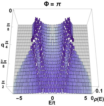
Figure 2: Three-dimensional plot of the density of states $\rho(E)$ (with the energy in units of $t$) as a function of the non-Abelian strength parameter $q$.

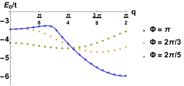
Figure 3: Single particle ground state energy $E_{0}$ (in units of $t$) as a function of $q$ for $m=1$ and $n=2,3,5$. The solid line is the exact analytical solution for $n=2$. The dots are obtained by evaluating the spectrum in a discretization of the BZ into $25^{3}$ points.

For $m=1$ and $n=2$ we limited ourself to the case $\vec{A}_{\text{NAB}}=q\,(\sigma_{x},\sigma_{y},\sigma_{z})$, but the previous results can be easily extended to non-Abelian anisotropic potentials of the form $\vec{A}_{\text{NAB}}=(q_{x}\,\sigma_{x},q_{y}\,\sigma_{y},q_{z}\,\sigma_{z})$. An interesting case is obtained when $q_{x}=q_{y}\equiv q$ and $q_{z}=0$, which has been studied in relation to the formation of a double-Weyl semimetal phase [55].

5.2 Abelian magnetic flux $\frac{2\pi}{3}$

We focus in this Subsection on the cases with isotropic magnetic flux $\Phi=\frac{2\pi}{3}$, breaking explicitly the physical time-reversal symmetry. We consider the same non-Abelian gauge potential entering (42), so that the full potential reads

$$\vec{A}=\vec{A}_{\text{AB}}+\vec{A}_{\text{NAB}}=\frac{2\pi}{3}\,(0,x-y,y-x)\otimes{\bf 1}+q\,(\sigma_{x},\sigma_{y},\sigma_{z})\,.$$ (59)

With $\Phi=\frac{2\pi}{3}$ the unit cell is composed of three sites, so it is useful to introduce a new pseudospin-$1$ degree of freedom with a diagonal operator labeled by $T_{z}^{\mathrm{AB}}$, whose diagonal entries characterize the $x$ coordinates of the lattices modulo $3$, as discussed in Section 3. Correspondingly, the MBZ is defined by the quasi-momenta $k_{x}\in\left[-\pi,\pi\right)$ and $k_{y},k_{z}\in\left[-\pi/3,\pi/3\right)$. By introducing the matrices

$$T_{\hat{x}}^{\mathrm{AB}}=\begin{pmatrix}0&0&1\\ 1&0&0\\ 0&1&0\end{pmatrix}\,,\quad T_{\hat{y}}^{\mathrm{AB}}=\begin{pmatrix}0&0&e^{-i\pi/3}\\ e^{i\pi/3}&0&0\\ 0&-1&0\end{pmatrix}\,\quad T_{\hat{z}}^{\mathrm{AB}}=\begin{pmatrix}1&0&0\\ 0&e^{i\frac{4\pi}{3}}&0\\ 0&0&e^{i\frac{2\pi}{3}}\end{pmatrix}\,,$$ (60)

the $6\times 6$ Hamiltonian in Eq. (17) reads in momentum space:

$$-\frac{H(\vec{k})}{t}=\cos q\cdot\sum_{\hat{j}}e^{-ik_{j}}T_{j}^{\mathrm{AB}}\otimes\sigma_{0}+i\sin q\cdot\sum_{\hat{j}}e^{-ik_{j}}T_{j}^{\mathrm{AB}}\otimes\sigma_{j}+{\rm H.c.}\,,$$ (61)

where $\hat{j}=\hat{x},\hat{y},\hat{z}$. To recast Eq. (61) in a form closer to Eq. (49), we write the matrices $T_{\hat{j}}^{\mathrm{AB}}$ as $T_{\hat{j}}^{\mathrm{AB}}=R_{\hat{j}}^{\mathrm{AB}}+S_{\hat{j}}^{\mathrm{AB}}$, where $R_{\hat{j}}^{\mathrm{AB}}$ is Hermitian and $S_{\hat{j}}^{\mathrm{AB}}$ is anti-Hermitian so that $R_{\hat{j}}^{\mathrm{AB}}=(T_{\hat{j}}^{\mathrm{AB}}+T_{\hat{j}}^{\mathrm{AB}{\dagger}})/2$ and $S_{\hat{j}}^{\mathrm{AB}}=(T_{\hat{j}}^{\mathrm{AB}}-T_{\hat{j}}^{\mathrm{AB}{\dagger}})/2$. In this way we can write Eq. (61) as

$$-\frac{H(\vec{k})}{2t}=\cos q\cdot{\cal H}_{0}+\sin q\cdot{\cal H}_{1}\,,$$ (62)

where

$${\cal H}_{0}=\sum_{\hat{j}}\left\{\cos{k_{j}}\left(R_{\hat{j}}^{\mathrm{AB}}\otimes\sigma_{0}\right)+\,\sin{k_{j}}\left(I_{\hat{j}}^{\mathrm{AB}}\otimes\sigma_{0}\right)\,\right\},$$ (63)

and

$${\cal H}_{1}=\sum_{\hat{j}}\left\{\sin{k_{j}}\left(R_{\hat{j}}^{\mathrm{AB}}\otimes\sigma_{j}\right)-\,\cos{k_{j}}\left(I_{\hat{j}}^{\mathrm{AB}}\otimes\sigma_{j}\right)\,\right\}\,,$$ (64)

where we introduced the Hermitian matrices $I_{\hat{j}}^{\mathrm{AB}}\equiv-iS_{\hat{j}}^{\mathrm{AB}}$. We expect the structure defined in Eqs. (62)–(64) to be valid for general values of $m$ and $n$. Moreover, the comparison between Eqs. (62)–(64) and Eqs. (49)–(51) show the peculiarity of the $\pi$-flux case, where the matrices $T_{\hat{j}}^{\mathrm{AB}}$ are Hermitian, so that $I_{\hat{j}}^{\mathrm{AB}}=0$ [indeed the matrices $T_{\hat{j}}^{\mathrm{AB}}$ are just the Pauli matrices for $m=1$ and $n=2$].

An interesting point to be noticed is that for $\Phi=\pi$ and $q=0$, the single particle ground state is obtained for $k_{x}=k_{y}=k_{z}=0$, giving $E_{0}=-2\sqrt{3}t$. For flux $2\pi/3$, choosing $q=0$ and setting $k_{x}=k_{y}=k_{z}=0$ one gets six energies, and the smallest is given by $-\frac{1}{2}\left(1+\sqrt{33}\right)t\approx-3.37t$, which appears to be above the single particle ground state energy $E_{0}$ found by diagonalizing Eq. (62) on all the MBZ without the restriction $|k_{x}|=|k_{y}|=|k_{z}|$. The position of the minimum in momentum space is a non-trivial problem and it is obviously related to the gauge choice. We observe indeed that by multiplying any of the $T_{\hat{j}}^{\mathrm{AB}}$ matrices by a phase, the spectrum is translated accordingly in momentum space, even though of course the values of the eigenenergies do not change. It would certainly be interesting to determine a choice of the gauge simplifying – or fixing, if such choice does exist – the determination of the position of the minimum.

Qualitatively, for $q=0$ the spectrum of the Hamiltonian (61) is composed of three doubly-degenerate bands, due to the absence of any spin term. These bands touch in points with a linear dispersion, possibly realizing a Weyl semimetal phase at fillings $2/3$ and $4/3$. This is reflected in the quadratic behavior of the density of states depicted in Fig. 4 around the two minima, at zero density for $q=0$, which separate the three degenerate bands. For $q>0$ the spectrum divides into six bands which are still connected, in general, by band-touching points but, otherwise, they do not intersect. For small values of $q$, the six bands do not overlap in energy, thus determining, in general, metallic phases, separated by semimetal phases at commensurate filling $n/3$. Above a critical value, though, the bands start to overlap and the system is in a metallic phase for any filling. Finally, for $q$ approaching $\pi/2$, the density of states becomes again suppressed in small energy ranges separating the bands. Also in this case, these regions do not correspond to gaps between the bands but to semimetallic phases with band touching points between them. We observe that the energy bands display no particular symmetries, as expected from the Hamiltonian in Eq. (61).

A similar picture emerges for larger $n$: e.g., for $m=1$ and $n=5$, corresponding to $\Phi=\frac{2\pi}{5}$. For $q=0$ five twofold-degenerate bands occur, that split in ten single bands at $q\neq 0$. The density of states $\rho(E)$ vanishes at isolated points along the lines $q=0$ and $q=\frac{\pi}{2}$. At the corresponding energies, we observe a linear band touching between neighboring bands.

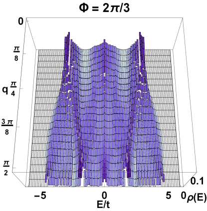
Figure 4: Density of states of the Hamiltonian in Eq. (61) as a function of the energy and the parameter $q$. For $q=0$ two regions with the DOS vanishing quadratically are particularly evident: they correspond to linearly dispersing band touching points.

6 The effect of flux perturbations

The definitions of the magnetic unit cell and Brillouin zone discussed in the previous Sections can be used to shed light on the behavior of systems with artificial gauge potentials in finite size systems, also when the Abelian fluxes are slightly perturbed around some key values, and, in particular, around a configuration where the Abelian potential defines $\pi$ fluxes for all the three orientations of the plaquettes of the cubic lattice.

In Refs. [22, 46] it was shown that the cubic lattice model with $\pi$ fluxes hosts a Weyl semimetal phase and in Ref. [45] we discussed the effect of small random perturbations around this value of the fluxes. Interestingly, the results for small system sizes are analogous to those obtained by the introduction of onsite disorder in solid-state realizations of Weyl semimetals [58, 59, 60, 61, 62, 63]. For small flux perturbations, the density of states of the system at low energy shows a deviation from the linear behavior typical of the Weyl semimetals, which is compatible with the introduction of rare localized states.

To address a specific and physically relevant example in the formalism introduced in the present paper, we can consider, in the thermodynamic limit, the system with random fluxes of the form $\pi(1\pm 1/p)$, with $p$ integer and $1/p$ a small perturbation around $\pi$. The system then display a fractal spectrum (see for example Refs. [38, 39, 40]), and the Weyl physics disappears. This leads to instabilities even for infinitesimal fluctuations of the Abelian flux, in a context that it is similar to its two-dimensional counterpart, described by the Hofstadter butterfly [5].

The introduction of the parameters $p_{i}$ in the three directions, however, causes the appearance of a volume scale given by the size of the magnetic unit cell, which grows with the least common multiple of the $p_{i}$ parameters, as dictated by Eq. (23). Therefore, the thermodynamic behavior describes only systems larger than this unit cell. For smaller sizes we will show in the following that the system is analogous to a collection of disordered two-dimensional models, which explains the physics of finite sizes and small perturbations.

To describe these systems in more detail, we consider the case of a gauge potential displaying $\pi$ magnetic fluxes along the three directions and a non-Abelian component which is gauge-equivalent to the common two-dimensional spin-orbit couplings (Rashba or Dresselhaus). We emphasize that such a non-Abelian term is analogous to the one recently experimentally realized with ${}^{40}K$ gases in continuum space [64], and a recent proposal paves the way for its realization in optical lattices [65]. The gauge potential reads

$$\vec{A}=\vec{A}_{\text{AB}}+\vec{A}_{\text{NAB}}=\pi\,(0,x-y,y-x)\,{\bf 1}+(q_{x}\sigma_{x},q_{y}\sigma_{y},0)\,,$$ (65)

with

$$U_{\hat{x}}=\exp\left({iq_{x}\,\sigma_{x}}\right)\,,$$ (66)

$$U_{\hat{y}}(x,y)=\exp\left[{i\,\pi\,\Big{(}x-y-\frac{1}{2}\Big{)}+iq_{y}\,\sigma_{y}}\right]\,,$$ (67)

$$U_{\hat{z}}(x,y)=\exp\left[{-i\,\pi\,\Big{(}x-y\Big{)}}\right]\,.$$ (68)

In the limit $q_{x},q_{y}\to 0$, the system describes a PT-invariant Weyl semimetal [45]. In the symmetric case $q_{x}=q_{y}$, in Ref. [55] it was shown that it corresponds to a double-Weyl semimetal, namely a gapless system in which the central bands touch in points whose dispersion is quadratic along $\hat{x}$ and $\hat{y}$ and linear along $\hat{z}$. Such band touching points are topological objects characterized by a double monopole of the Berry curvature and they are protected by the $C_{4}$ rotational symmetry of the system [66]. By introducing an anisotropy with $q_{x}\neq q_{y}$, the double-Weyl points split into pairs of Weyl cones with the same charge.

To understand the role of the Abelian flux perturbations in the cubic lattice model it is convenient to use the following gauge choice for the Abelian component of the vector potential:

$$\vec{A}_{AB}=\left(0,\gamma x-\pi y,\alpha y-\beta x\right)\,.$$ (69)

This Abelian component corresponds to a generalization of the Abelian contribution in Eq. (27) such that the magnetic fluxes are $(\alpha,\beta,\gamma)$, corresponding to a generic choice of the $U(1)$ fluxes in all the plaquettes of the cube. The potential in Eq. (69) does not depend on the $z$ coordinate due to this gauge choice. This allows us to consider the tight-binding Hamiltonian obtained from this perturbation of the fluxes and the Rashba-like spin-orbit coupling in Eq. (65) as a function of the real space coordinates $x,y$ and the momentum $k_{z}$, which may be thought of as a parameter labeling different two-dimensional systems in the $xy$ plane.

Therefore, we can rewrite the Hamiltonian as:

$$H=-\sum_{k_{z}}\sum_{x,y}\left\{\left[t_{\hat{x}}U_{\hat{x}}(x,y)c^{\dagger}_{x+\hat{x},y,k_{z}}c_{x,y,k_{z}}+t_{\hat{y}}U_{\hat{y}}(x,y)c^{\dagger}_{x,y+\hat{y},k_{z}}c_{x,y,k_{z}}+{\rm H.c.}\right]+\right.\\ +\left.2t_{\hat{z}}\cos\left(k_{z}+\alpha y-\beta x\right)c^{\dagger}_{x,y,k_{z}}c_{x,y,k_{z}}\right\}\,,$$ (70)

where the unitary operators $U_{\hat{x}}$ and $U_{\hat{y}}$ include both the action of the Abelian flux $\gamma$ piercing the plaquettes of the two-dimensional $x-y$ system and the non-Abelian hopping operators along the $x,y$ directions:

$$U_{\hat{x}}=e^{iq_{x}\sigma_{z}}\,,\quad U_{\hat{y}}=e^{i\left(\gamma x-\pi y-\frac{\pi}{2}\right)+iq_{y}\sigma_{y}}\,.$$ (71)

These operators describe the kinetic contribution of the two-dimensional Hamiltonian. The last term in Eq. (70) can be considered as an onsite potential in the plane $x-y$ oscillating in space and depending on the values of $\alpha$ and $\beta$, with $k_{z}$ being just a phase for this periodic potential. This oscillating potential characterizes as well the so-called Aubry-André model [8]. When $\alpha$ and $\beta$ are incommensurate with the optical lattice spacing, the Hamiltonian (70) describes a two-dimensional system of particles subject to $\pi$ fluxes and spin-orbit coupling and moving in a quasi-periodic system. In this incommensurate regime, the previous potential can drive a transition from extended to localized states.

In finite systems, commensurate potentials may show the same behavior as incommensurate ones, when their spatial period is large compared to the system size. We consider here what happens if $\alpha$ and $\beta$ are weakly perturbed around the original value $\pi$. We assume their value is of the kind $\alpha,\beta=\pi(1\pm 1/p_{\alpha/\beta})$ with odd integers $p_{\alpha},p_{\beta}\gg 1$. The spatial period of the onsite potential in the plane becomes $p_{\alpha}$ in the $\hat{y}$ direction and $p_{\beta}$ along $\hat{x}$. Therefore, if the system has a size $L_{x,y}\ll p_{\beta,\alpha}$, the system cannot be truly considered in the thermodynamic limit because its size is considerably smaller that the period of the onsite potential, and its phenomenology reproduces the one of an incommensurate potential. This effect has been experimentally investigated with Bose-Einstein condensates [67], where it was shown that the introduction of a quasi-periodic potential on a finite system can indeed cause a crossover to a regime with localized states.

Therefore, for small perturbations of the Abelian fluxes on a finite system, the Hamiltonian in Eq. (70) can be considered, for each value of $k_{z}$, as a two-dimensional Hofstadter model with flux $\gamma$ and spin orbit terms dictated by $U_{\hat{x}}$ and $U_{\hat{y}}$ [57] with the addition of an effective on-site disorder, characterized by the phase $k_{z}$. This qualitatively explains the appearance of a diffusive phase in the perturbed Abelian system [45], behaving analogously to a disordered Weyl semimetal and characterized by the appearance of rare quasi-localized states [58]. We observe that this mapping from a three-dimensional cubic lattice model with fluxes to a two-dimensional square lattice model with a quasi-periodic potential follows the usual mapping from the two-dimensional Harper model to the one-dimensional Aubry-André model. In the following we study the stability of the energy spectrum in presence of gauge fluctuations.

6.1 Stability of the energy spectrum against gauge fluctuations

As shown in the previous Sections, a translationally invariant non-Abelian potential does not change the size of the MBZ. This fact has important consequences on the stability of the Weyl semimetal phase to non-Abelian gauge fluctuations, such as variations of $q_{x,y}$ in Eq. (65).

In the presence of a purely non-Abelian coupling, obtained by imposing $m=0$ in Eq. (27), all the operators $U$ loose their space-dependence and the MBZ coincides with the usual BZ induced by the geometric shape of the lattice. Therefore, no qualitative deviation from the spectrum at $L\to\infty$ is expected in the presence of small perturbations of the coefficients $q_{i}$. Moreover, the spectrum changes continuously with the strength of the non-Abelian component and no fractal structure is found. For this reason we expect a substantial stability of the spectrum against small fluctuations $\delta q_{x,y}$ of the non-Abelian gauge potential.

Instead, when both an Abelian and a uniform non-Abelian couplings are involved, the MBZ size is the same as in the purely Abelian case, so that a fractal instability in the limit $L\to\infty$ occurs from the Abelian contribution only. This expectation can be directly probed directly for the system described by Eq. (70), where a double-Weyl semimetal phase appears. These semimetals are protected by a $C_{4}$ symmetry [66] and characterized by isolated band touching points between two bands. In the same points the dispersion is quadratic along two momentum directions and linear along the third one, so that they are characterized by a linearly vanishing density of states.

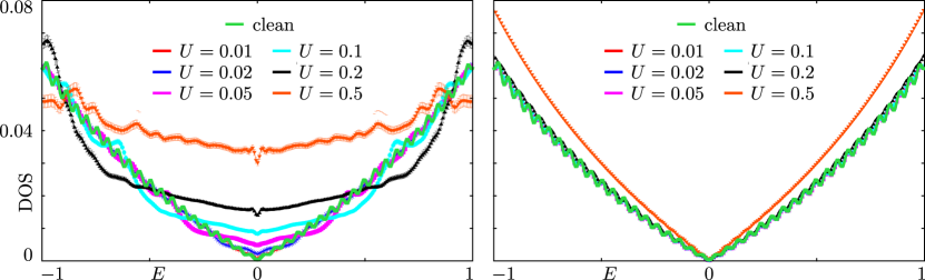
Figure 5: Average density of states $\rho$ as a function of energy (in units of $t$) around the double-Weyl points for random fluctuations of the flux $\Phi$ around $\pi$ (left panel) or $q_{x,y}$ around $\pi/4$ (right panel). Different colors denote the strength of the fluctuations, $U$. For $U=0$, $\rho$ is linear around the double-Weyl point energy ($E=0$) in both cases. In the left panel, a flat region of nonzero density of states develops even for small values of $U$, signaling the destruction of the semimetal phase. In the right panel, $\rho$ remains linear also for large values of $U$, such that the double-Weyl semimetal is robust to fluctuations in the non-Abelian potential only.

In Fig. 5 the stability of the band-touching points against fluctuations of the Abelian flux $\delta\Phi$ and of the non-Abelian strengths $\delta q_{x,y}$ is investigated (left and right panel, respectively), for a cubic system of linear size $L=120$. The fluctuations are randomly and independently drawn from the uniform distribution $[-U,U]$ around the values $\Phi=\pi$ and $q_{x}=q_{x}=\pi/4$. We show the density of states at energies around the band touching points, calculated by averaging over $200$ independent random potential configurations at fixed disorder strength $U$, using a kernel polynomial approximation with $N=1024$ polynomials, and a stochastic evaluation of the trace with $R=10$ random vectors (for details on the method, see Ref. [45]). In the absence of fluctuations, the density of states shows the expected linear profile around the band touching points.

At fixed $q_{x}=q_{y}=\pi/4$ and adding fluctuations in $\Phi$, we find that the density of states at the energy of the double Weyl points rapidly develops a plateau as $U$ increases, signaling the breakdown of the double-Weyl semimetal. The situation in very similar a to the one described in Ref. [55] for the purely Abelian $\pi$ flux cubic lattice model. At variance, at fixed $\Phi=\pi$ and for fluctuating $q_{x,y}$ the density of states remains linear also for larger values of $U$. These results support our expectation on the stability of the spectra against fluctuation of the gauge potentials, based on the discussion on the properties of the MBZ presented above.

7 Conclusions

In this work we presented the general analytic formalism to solve tight-binding models describing particles in a cubic lattice subject to translational invariant Abelian and non-Abelian gauge potentials. We considered the general case of commensurate magnetic fluxes, possibly different along the three directions.

We then discussed several examples related to $U(2)$ potentials, as systems with a Rashba-like coupling, also relevant for the realization of particular topological semimetals [55]. There we also investigated the effects of perturbing the magnetic fluxes.

Our study illustrates the interexchange between the formal techniques developed to describe lattice particles in magnetic fields and the advancements coming from the simulation of tunable gauge potentials in ultracold atom experiments. These adavancements motivate the exploration of the mathematical structure of the single particle energy spectrum in new situations, such as in the presence of non-Abelian gauge potentials.

We showed in particular that the Hasegawa gauge, in the presence of a commensurate Abelian flux $\Phi=2\pi\frac{m}{n}$, reduces the problem in the momentum space to the diagonalization of a $n\times n$ matrix for the purely Abelian case, and of a $pn\times pn$ matrix if the particle has $p$ degrees of freedom (more generally of the system has $p$ components). Exploiting this formalism, one can study the case of vanishing flux $\Phi\to 0$ (i.e., $n\to\infty$) or the dependence of the energy spectrum on the parameters of the translational invariant non-Abelian gauge potential, such as $q$ for the potential $\vec{A}_{\text{NAB}}=q\,(\sigma_{x},\sigma_{y},\sigma_{z})$, that we considered in Section 5.

Our study also offers useful tools for the design and analysis of ultracold atom and photonic platforms for the realization of exotic topological phases of matter, often relying on artificial gauge potentials, and it provides interesting alternative routes for the implementation of novel quantum phenomena. On the technical level, the approach described here can be generalized also to the case of magnetic fluxes which vary periodically across the lattice and it can be also extended to the simulations of the so-called extra dimensions [26], a topic recently at the center of many discussions in the quantum simulation community, for instance concerning the experimental realization of 4D quantum Hall systems [68, 69].

References

References

- [1] Y. Aharonov and D. Bohm, Phys. Rev. 115, 485 (1959).
- [2] I. Z̆utić, J. Fabian and S. Das Sarma, Rev. Mod. Phys. 76, 323 (2004).
- [3] D. Yoshioka, The quantum Hall effect (Berlin, Springer-Verlag, 2002).
- [4] M. Ya. Azbel, Sov. Phys. JETP 19, 634 (1964).
- [5] D. R. Hofstadter, Phys. Rev. B 14, 2239 (1976).
- [6] P. G. Harper, Proc. Phys. Soc. A 68, 874 (1955).
- [7] D. J. Thouless, The Quantum Hall Effect and the Schrödinger Equation with Competing Periods, pp. 170-176 in [70].
- [8] S. Aubry and G. André, Ann. Israel Phys. Soc. 3, 133 (1980).
- [9] D. J. Thouless, M. Kohmoto, M. P. Nightingale, and M. den Nijs, Phys. Rev. Lett. 49, 405 (1982).
- [10] X.-L. Qi and S.-C. Zhang, Rev. Mod. Phys. 83, 1057 (2011).
- [11] M. Z. Hasan and C. L. Kane, Rev. Mod. Phys. 82, 3045 (2010).
- [12] A. P. Schnyder, S. Ryu, A. Furusaki and A. W. W. Ludwig, Phys. Rev. B 78, 195125 (2008).
- [13] I. Bloch, J. Dalibard and W. Zwerger, Rev. Mod. Phys. 80, 885 (2008).
- [14] M. Lewenstein, A. Sanpera and V. Ahufinger, Ultracold atoms in optical lattices: simulating quantum many-body systems (Oxford, Oxford University Press, 2012).
- [15] J. Dalibard, F. Gerbier, G. Juzeliūnas and P. Öhberg, Rev. Mod. Phys. 83, 1523 (2011).
- [16] N. Goldman, G. Juzeliūnas, P. Öhberg and I. B. Spielman, Rep. Prog. Phys. 77, 126401 (2014).
- [17] M. Burrello, L. Lepori, S. Paganelli and A. Trombettoni, Abelian gauge potentials on cubic lattices, to appear in [18].
- [18] Advances in Quantum Mechanics: Contemporary Trends and Open Problems, G. Dell’Antonio and A. Michelangeli eds. (Springer-INdAM series, 2017).
- [19] D. Jaksch and P. Zoller, New. J. Phys. 5, 56 (2003).
- [20] M. Aidelsburger, M. Atala, M. Lohse, J. T. Barreiro, B. Paredes and I. Bloch, Phys. Rev. Lett. 111, 185301 (2013).
- [21] A. Bermudez, L. Mazza, M. Rizzi, N. Goldman, M. Lewenstein and M. A. Martin-Delgado, Phys. Rev. Lett. 105, 190404 (2010).
- [22] L. Lepori, G. Mussardo and A. Trombettoni, Europhys. Lett. 92, 50003 (2010).
- [23] Z. Lan, N. Goldman, A. Bermudez, W. Lu and P. Öhberg, Phys. Rev. B 84, 165115 (2011).
- [24] L. Tarruell, D. Greif, T. Uehlinger, G. Jotzu and T. Esslinger, Nature 483, 302 (2012).
- [25] L. Lepori, A. Celi, A. Trombettoni and M. Mannarelli, arXiv:1708.00281.
- [26] O. Boada, A. Celi, J. I. Latorre and M. Lewenstein, Phys. Rev. Lett. 108, 133001 (2012).
- [27] M. Mancini, G. Pagano, G. Cappellini, L. Livi, M. Rider, J. Catani, C. Sias, P. Zoller, M. Inguscio, M. Dalmonte and L. Fallani, Science 349, 6255 (2015).
- [28] B. K. Stuhl, H.-I. Lu, L. M. Aycock, D. Genkina and I. B. Spielman, Science 349, 1514 (2015).
- [29] M. Burrello and A. Trombettoni, Phys. Rev. Lett. 105, 125304 (2010); Phys. Rev. A 84, 043625 (2011).
- [30] G. Juzeliūnas, J. Ruseckas, M. Lindberg, L. Santos and P. Öhberg, Phys. Rev. A 77, 011802(R) (2008).
- [31] L.-K. Lim, C. M. Smith, and A. Hemmerich, Phys. Rev. Lett. 100, 130402 (2008).
- [32] J.-M. Hou, W.-X. Yang and X.-J. Liu, Phys. Rev. A 79, 043621 (2009).
- [33] I. Affleck and J. B. Marston, Phys. Rev. B 37, 3774 (1988).
- [34] Y. Hasegawa, J. Phys. Soc. Jap. 59 4384 (1990); Physica C 185-189, 1541 (1991).
- [35] R. B. Laughlin and Z. Zou, Phys. Rev. B 41, 664 (1990).
- [36] G. Mazzucchi, L. Lepori and A. Trombettoni, J. Phys. B: At. Mol. Opt. Phys. 46 134014 (2013).
- [37] E. M. Lifschitz and L. P. Pitaevskii, Statistical Physics, Part 2 (Pergamon Press, 1980).
- [38] Z. Kunszt and A. Zee, Phys. Rev. B 44, 6842 (1991).
- [39] M. Koshino, H. Aoki, K. Kuroki, S. Kagoshima and T. Osada, Phys. Rev. Lett. 86, 1062 (2001).
- [40] M. Koshino and H. Aoki, Phys. Rev. B 67, 195336 (2003).
- [41] Y.-L. Lin and F. Nori, Phys. Rev. B 53, 13374 (1996).
- [42] H. J. Rothe, Lattice gauge fields: an introduction (Singapore, World Scientific, 2005).
- [43] M. E. Peskin and D. V. Schroeder, An Introduction To Quantum Field Theory (Reading, Addison-Wesley, 1995).
- [44] L. D. Landau and E. M. Lifschitz, Quantum Mechanics (Pergamon Press, 1965).
- [45] L. Lepori, I. C. Fulga, A. Trombettoni and M. Burrello, Phys. Rev. B. 94, 085107 (2016).
- [46] T. Dubcek, C. J. Kennedy, L. Lu, W. Ketterle, M. Soljacic and H. Buljan, Phys. Rev. Lett. 114, 225301 (2015).
- [47] H. Georgi, Lie Algebras in Particle Physics ( Reading, Perseus Books, 1999).
- [48] S. Weinberg, The quantum theory of fields, Vol. 2 (Cambridge, Cambridge University Press, 1996).
- [49] P. M. Fishbane, S. Gasiorowicz and P. Kaus, Phys. Rev. D 24, 2324 (1981).
- [50] S. Lang, Linear Algebra (Springer, 1987).
- [51] J. P. Vyasanakere, S. Zhang and V. B. Shenoy, Phys. Rev. B 84, 014512 (2011).
- [52] C.-K. Chiu, J. C.Y. Teo, A. P. Schnyder and S. Ryu, Rev. Mod. Phys. 88, 035005 (2016).
- [53] J. Armaitis, J. Ruseckas and G. Juzeliūnas, Phys. Rev. A 95, 033635 (2017).
- [54] B. M. Anderson, G. Juzeliūnas, V. M. Galitski and I. B. Spielman, Phys. Rev. Lett. 108, 235301 (2012).
- [55] L. Lepori, I. C. Fulga, A. Trombettoni and M. Burrello, Phys. Rev. A 94 053633 (2016).
- [56] N. Goldman, A. Kubasiak, P. Gaspard and M. Lewenstein, Phys. Rev. A 79, 023624 (2009).
- [57] M. Burrello, I. C. Fulga, E. Alba, L. Lepori and A. Trombettoni, Phys. Rev. A 88, 053619 (2013).
- [58] J. H. Pixley, D. A. Huse and S. Das Sarma, Phys. Rev. X 6, 021042 (2016).
- [59] B. Sbierski, G. Pohl, E. J. Bergholtz, and P. W. Brouwer, Phys. Rev. Lett. 113, 026602 (2014).
- [60] B. Sbierski, M. Trescher, E. J. Bergholtz, and P. W. Brouwer, Phys. Rev. B 95, 115104 (2017).
- [61] M. Trescher, B. Sbierski, P. W. Brouwer, and E. J. Bergholtz, Phys. Rev. B 95, 045139 (2017).
- [62] S. Bera, J. D. Sau, and B. Roy, Phys. Rev. B 93, 201302 (2016).
-
[63]
B. Roy, R.-J. Slager, and V. Juricic,
arXiv:1610.08973 - [64] L. Huang, Z. Meng, P. Wang, P. Peng, S.-L. Zhang, L. Chen, D. Li, Q. Zhou and J. Zhang, Nature Phys. 12, 540 (2016).
- [65] F. Grusdt, T. Li, I. Bloch and E. Demler, Phys. Rev. A 95, 063617 (2017).
- [66] C. Fang, M. J. Gilbert, X. Dai and B. A. Bernevig, Phys. Rev. Lett. 108, 266802 (2012).
- [67] G. Roati et al., Nature 453, 895 (2008).
- [68] H. M. Price, O. Zilberberg, T. Ozawa, I. Carusotto and N. Goldman, Phys. Rev. Lett. 115, 195303 (2015).
-
[69]
M. Lohse, C. Schweizer, H. M. Price, O. Zilberberg and I. Bloch,
arXiv:1705.08371 - [70] Number Theory and Physics, Springer Proceedings in Physics, Vol. 47, J. M. Luck, P. Moussa and M. Waldschmidt eds. (Berlin, Springer-Verlag, 1990).