Probing homogeneity with standard candles

Abstract

We show that standard candles can provide some valuable information about the density contrast, which could be particularly important at redshifts where other observations are not available. We use an inversion method to reconstruct the local radial density profile from luminosity distance observations assuming background cosmological parameters obtained from large scale observations. Using type Ia Supernovae, Cepheids and the cosmological parameters from the Planck mission we reconstruct the radial density profiles along two different directions of the sky. We compare these profiles to other density maps obtained from luminosity density, in particular Keenan et al. 2013 and the 2M++ galaxy catalogue. The method independently confirms the existence of inhomogeneities, could be particularly useful to correctly normalize density maps from galaxy surveys with respect to the average density of the Universe, and could clarify the apparent discrepancy between local and large scale estimations of the Hubble constant. When better observational supernovae data will be available, the accuracy of the reconstructed density profiles will improve and will allow to further investigate the existence of structures whose size is beyond the reach of galaxy surveys.

1 Introduction

The standard cosmological model has reached a high level of accuracy and self-consistency, accommodating in one unified theoretical framework different types of observations such as the cosmic microwave background (CMB), type Ia supernovae (SNe) and baryon acoustic oscillations (BAO). The population of SNe, historical probe of the cosmological constant $\Lambda$, is now comprising a large number of objects with 740 spectroscopically confirmed ones at redshifts $0.05<z<1.0$ (c.f. [1]). Thanks to many progresses, the precision on cosmological parameters is now approaching the percent level. Nevertheless, one parameter seems to create controversy in this consistent picture by showing a 2-3$\sigma$ tension between the different probes, and this is today’s Hubble parameter $H_{0}$. Recently in Riess et al. ([2], abbreviated as $\mathcal{R}$16) $H_{0}$ was re-evaluated with the best Cepheid calibration so far (details in [3, 4]), and it was found $H_{0}=73.24\pm 1.74$ ${\rm km\,s^{-1}\,{\rm Mpc}^{-1}}$, hence raising the tension to $3.4\sigma$ against the $66.93\pm 0.62$ ${\rm km\,s^{-1}\,{\rm Mpc}^{-1}}$ value derived from the CMB observation of Planck [5], denoted in the rest of the paper as $\rm Planck$. It is thus important to explain this discrepancy.

Several ideas have been tested against data in order to resolve this problem. One possibility is to modify our early-time picture of the Universe by changing our interpretation of CMB measurements [6]. It has also been proposed that the tension itself needs to be reinterpreted (c.f. [7]).

A more conservative idea is to consider that different probes do not measure the same $H_{0}$. In this spirit, inhomogeneous geometries have been tested with SNe data from the very start [8, 9], with perturbative [10, 11] and non-perturbative models like the Lemaître-Tolman-Bondi (LTB) model [12, 13, 14, 15, 16, 17] or the swiss-cheese model [18, 19]. However, viable models must explain not only the magnitudes of SNe, but also pass constraints from other cosmological probes [20, 21, 22, 23, 15].

It has been shown that [24] in the linear pertubative regime local inhomogeneities could resolve the apparent tension as the distance to the last scattering surface in negligibly affected by local structures, while at low redshift the local estimation of $H_{0}$ can be strongly affected. In the non perturbative regime the distance to the last scattering can be significantly affected by a local inhomogeneity, and in this case both the effects on local and large scale observations should be taken into account in order to determine if the tension can be partially resolved. In order to differentiate between the two measurements, from now on we denote the local value of the Hubble parameter as $H_{0}^{\rm loc}$, and the large scale value as $H_{0}^{\rm LS}$.

The statistical estimation of how much the $H_{0}^{\rm loc}$ value could vary among different regions of the Universe due to inhomogeneities was studied in [25] and more recently in [11, 26], where it was shown that there could be an uncertainty on $H_{0}^{\rm loc}$ of the same order of its current experimental errors. Nevertheless it should be noted that all these “cosmic variance” analyses involve an angular average which may underestimate the effects of anisotropy of local structure. Anisotropic effects could in fact play an important role [24, 27, 28] because of the anisotropic distribution of SNe, even if the angular average of the effects on $H_{0}^{\rm loc}$ is not large enough to explain the tension.

This directional effect is mainly due to the assumption made in $\mathcal{R}$16 that the effect of inhomogeneities has been fully removed by the redshift correction based on 2M++ density map. This is not necessarily the case as the density maps used to perform the correction are limited by the observational depth. Notice that an isotropic inhomogeneity extending in all directions beyond the depth of 2M++ density map is unlikely according to the $\Lambda$CDM structure formation predictions. However, an anisotropic inhomogeneity extending only in some directions where most of SNe are located is a different case, and the probability estimation for the existence of such anisotropic inhomogeneities requires further investigations.

Local inhomogeneities explaining the tension between $H_{0}^{\rm loc}$ and $H_{0}^{\rm LS}$ could be tested independently using local density measurements and may also be related to the tensions in the estimation of the density parameter $\Omega_{m0}$ and the amplitude of the linear power spectrum $\sigma_{8}$ (c.f. [29, 30]). Considerable progress has been achieved in studying the bulk flow (e.g. [31, 32, 33, 34]), with most studies converging on a velocity of several hundreds of ${\rm km\,s^{-1}}$ in a direction close to the CMB dipole of [35]: $384\pm 78\,{\rm(stat)}\pm 115\,{\rm(syst)}$ ${\rm km\,s^{-1}}$ pointing to the direction $(l,b)=(264^{\circ},48^{\circ})$ in galactic coordinates.

Analyses are in general consistent with the $\Lambda$CDM model[36, 37] and it is well established observationally the existence of inhomogeneities extending in some directions up to a few hundred megaparsecs [38, 20, 39]. In particular, Keenan et al. ([39], abbreviated as $\mathcal{K}$13) reports an under-density in some direction of the sky that extends up to $z\sim 0.07$ and suggests that a rescaling of the density map derived from the 2M++ catalogue [40] is necessary. Direct measurements of $H(z)$ will probably help constraining $H_{0}$ in the future as well (c.f. [41, 42, 43]).

In this paper we improve and apply the inversion method derived in [24] and [44] to obtain the local density map from standard candles luminosity distance observations. The inversion method requires as input a smooth function for the luminosity distance $D_{L}(z)$ which we obtain with a model independent fit of a combination of Cepheids-hosting galaxies from $\mathcal{R}$16 and low redshift ($z<0.4$) SNe from the Union 2.1 catalogue of [45]. The fit is based on radial basis functions (RBFs) and MCMC sampling. Because we are interested in a possible angular dependence of data and we want to establish a comparison with galaxy surveys, we consider 3 fields of view (F1,F2,F3) from $\mathcal{K}$13, to which we compare our results. All SNe in a given field give rise to a radial profile averaging over the corresponding window. Assuming that lensing effects can be neglected relative to peculiar velocities [46], which is expected to be a valid approximation at small redshift [47], we reconstruct the radial density profile for each field based on the inversion method described in [44], with some modifications necessary to take into account the corrections to the growth rate due to the cosmological constant.

As the analyzed SNe are at small redshift, we also account for their galaxy plane motion by adding a constant 250 ${\rm km\,s^{-1}}$ velocity dispersion on SNe, and by comparing our results with $\mathcal{K}$13 and 2M++. We also consider the velocity dispersion of Cepheids-hosting galaxies and show that its effect is negligible, and that the fit quality is acceptable even without it, contrary to the assumption made in $\mathcal{R}$16.

Our work reveals that in one field of view (F1) there is an under-density whose effect can partially account for the $H_{0}$ estimation discrepancy, due to the large number of low redshift SNe located along that direction. The reconstructed density profile is in agreement with 2M++ rescaled according to $\mathcal{K}$13. The reconstructed density profile along F3 also shows the presence of a large under-density in agreement with rescaled 2M++.

Our results show that SNe data can be a unique tool to probe structures whose size is larger than the depth of other observations such as the galaxy catalogues. Any deviation of cosmological parameters from their large scale estimation can consequently be interpreted as the evidence of structures whose size is beyond the reach of presently available astronomical data from which peculiar velocities and associated redshift corrections are derived. Once more SNe data will become available, they could be a valuable source of information about large scale structures and especially for the correct estimation of background density, complementary to the density maps from galaxy surveys.

The paper is organized as follows. In section 2 we present the data employed in this study. This includes supernovae from the Union 2.1 catalogue, the latest Cepheids from $\mathcal{R}$16, and the 2M++ catalogue. In section 3 we explain the theoretical framework in which we interpret the data and describe the methods adopted in our statistical and numerical analysis. Section 4, 5 and 6 are devoted to the presentation of our results, the physical interpretations and the comparison with the analyses of $\mathcal{K}$13, $\mathcal{R}$16 and 2M++. In section 7 we present some further discussions about the results, their limitations and possible improvements. In section 8 we summarize our conclusions. Complementary results and our dataset are presented in appendices A, B, C and D.

2 Data

We are interested in the effects of inhomogeneities on the luminosity distance of low-redshift SNe and Cepheids-hosting galaxies, referred together as standard candles. At low redshift peculiar velocity can be important and produce an important contamination of the Hubble flow, and we will indeed devote a lot of attention to the problem of distinguishing appropriately between them. Two different sources of the peculiar velocity are investigated. First for the velocity dispersion within the bounded structures, unlike the 250 ${\rm km\,s^{-1}}$ dispersion universal to all standard candles in $\mathcal{R}$16, we differentiate between SNe and Cepheids-hosting galaxies. Second, for the bulk flow due to large scale inhomogeneities we reconstruct the density map from the luminosity distance of standard candles, and compare it with the map obtained from galaxy catalogues to test their consistency.

2.1 Supernovae Ia and Cepheids-hosting galaxies

The supernovae dataset is extracted from the full Union 2.1 catalogue of [45] (Supernova Cosmology Project) with a redshift cut $z<z_{\rm max}$, where $z_{\rm max}$ is either 0.2 or 0.4 (for reasons explained in section 2.2), and the exclusion of “bad” data points corresponding to types ‘p’, ‘f’ and ‘d’ respectively: bad light curve fittings, long first phases after B-band maximum and SNe observed only less than 5 times (c.f. [48], table 13 therein). For other types among the remaining SNe, we give a more detailed account in appendix D. We additionally remove 3 SNe with unconventional names, for which we cannot find the sky positions (see after), and rename two others . Concerning the redshift $z$, distance modulus $\mu$ and its error $\Delta\mu$, we prefer the values from the short Union 2.1 list (more precise), otherwise we take them from the full catalogue (less precise). To this dataset consisting of 288 ($z_{\rm max}=0.2$) or 372 ($z_{\rm max}=0.4$) SNe, we add 20 Cepheids-hosting galaxies from table 5 of $\mathcal{R}$16. Except the masers-hosting anchor NGC 4258, each of Cepheids-hosting galaxies also hosts a type Ia supernova, among which 7 SNe can be found in Union 2.1 (though only 3 in the fields we considered, see after). We use the redshift of the host galaxies given from the Ned database.

We are interested in the possible angular dependence of SNe due to local inhomogeneities. To study this dependence we consider 3 fields of view employed by $\mathcal{K}$13, to which we will compare our results. These fields are defined in table 1, shown in figure 1, and their total area of 6172 ${\rm deg}^{2}$ contains about half of the SNe. We extract the sky positions of all the Union 2.1 SNe and $\mathcal{R}$16 Cepheids-hosting galaxies automatically from the Simbad database of [50]. These positions are right ascension (R.A.) and declination (Dec.) expressed in the International Celestial Reference System (ICRS), written in decimal (degrees). We find more precisely for $z_{\rm max}=0.2$ ($z_{\rm max}=0.4$) that only 123 (203) SNe out of the 288 (372) Union 2.1 SNe are present in Fields 1, 2, and 3, as shown in table 1 and illustrated in figure 1. As we can see only Fields 1 and 3 (abbreviated as “F1” and “F3”) have enough data to be exploited, hence Field 2 (“F2”) is excluded from our analysis. Among all these SNe, 1 in F2 and 2 in F3 belong to the Cepheids-hosting galaxies of $\mathcal{R}$16 (denoted as “+1” and ”+2”). These 3 SNe will be considered as independent data points from the host in the statistical analysis, for the reasons discussed at the end of this subsection and at the beginning of section 2.2. Cepheids-hosting galaxies associated to these 3 SNe are denoted through their type by ‘$\ast$’ in appendix D. There are five other Cepheids-hosting galaxies in the fields we are interested in (1 in F1, 4 in F3) whose associated SNe are not included in Union 2.1, and they are denoted by ‘$\dagger$’ in appendix D.

Field	ICRS coordinates ($\rm deg$)		Number of SNe		Cepheids-hosting
N∘	R.A.	Dec.	$z_{\rm max}=0.2$	$z_{\rm max}=0.4$	galaxies of $\mathcal{R}$16
1	$[300,360]\cup[0,80]$	$[-3,4]$	69	144	1
2	$[130,250]$	$[-3,2]$	4+1	4+1	1
3	$[110,255]$	$[2,36]$	47+2	52+2	6
/	Whole Sky		288	372	20

Table 1: Fields of $\mathcal{K}$13 and number of standard candles they contain from our dataset. $[A,B]$ stands for the angular range between A and B (including the boundaries).

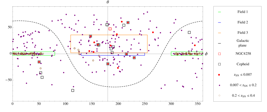
Figure 1: Sky map in ICRS coordinates of all SNe and Cepheids-hosting galaxies in our dataset. Three fields are specified according to $\mathcal{K}$13 as the regions with luminosity density data. Our targets of interest are F1 and F3 which contain enough data points to fit the luminosity distance curve. For the sake of clarity we use (here and later on) the same colors as $\mathcal{K}$13, i.e. green for F1 and orange for F3.

The Union 2.1 data contains no information about the absolute SNIa magnitudes. For this reason we convert the relative Union 2.1 magnitudes into absolute magnitudes by calibrating with the 7 SNe common to the $\mathcal{R}$16 and Union 2.1 datasets. It should be noted that the light curves fits of Union 2.1 are obtained assuming a homogeneous model, and a full model independent analysis would require to also include the effects of inhomogeneities in the light curves fits or to consider different types of fitters [51, 52, 53], but this would go beyond the scope of this paper. At low redshift the distance-modulus is given by

$$\mu\equiv m-M=25-5\log_{10}H_{0}^{\rm loc}+5\log_{10}\left(H_{0}^{\rm loc}D_{L}\right)\approx 25-5\log_{10}H_{0}^{\rm loc}+5\log_{10}cz\quad,$$ (2.1)

where $H_{0}^{\rm loc}$ is the local Hubble parameter fitted with low-redshift standard candles. Keeping the redshift fixed, we expect

$$\mu(\text{$\mathcal{R}${16}})=\mu(\text{{Union 2.1}})-5\log_{10}\left(\frac{73.24}{70}\right)\;\,.$$ (2.2)

This is what we obtain by fitting $\mu(\text{{Union 2.1}})-\mu(\text{$\mathcal{R}${16}})$ with a difference of $5\log_{10}\left(73.24/H_{0}^{\rm U2.1}\right)$ (where $H_{0}^{\rm U2.1}$ is the only parameter of the fit), based on the 7 SNe common to $\mathcal{R}$16 and Union 2.1, and weighted by $\Delta\mu^{2}(\text{{Union 2.1}})+\Delta\mu^{2}(\text{$\mathcal{R}${16}})$, as shown in figure 2. More precisely, we find $H_{0}^{\rm U2.1}=70.05\pm 2.20\,\rm{km\,s^{-1}\,{\rm Mpc}^{-1}}$, very close to the value 70 $\rm{km\,s^{-1}\,{\rm Mpc}^{-1}}$ assumed by Union 2.1 (and the value we keep). The uncertainty of the calibration is propagated to the covariance matrix $\tilde{V}$ of the shifted distance modulus of Union 2.1 SNe with components given by

$$\tilde{V}_{ij}=\Delta\mu_{i}^{2}(\text{{Union 2.1}})\,\delta_{ij}+\text{Variance}\left(\mu(\text{{Union 2.1}})-\mu(\text{$\mathcal{R}${16}})\right)\,.$$ (2.3)

In the remaining of this paper we will denote as $\mu$ the combination of shifted Union 2.1 SNe and $\mathcal{R}$16 Cepheids-hosting galaxies data, as $V^{-1}$ the inverse covariance matrix of the combined data, and as $\Delta\mu^{-2}$ the diagonal part of $V^{-1}$..

Figure 2: $\mu(\mbox{$\mathcal{R}${16}})$ - $\mu(\rm{Union~{}2.1})$ plot with 7 host galaxies common to $\mathcal{R}$16 Cepheids and Union 2.1 SNe. The black line represents the shift of $5\log_{10}\left(73.24/H_{0}^{\rm U2.1}\right)$ according to eq. (2.2).

Despite that the $\mathcal{R}$16 measurements of the distance modulus are almost the same as the corrected Union 2.1 moduli in eq. (2.2) (difference always $<0.3$ mag among the 7 SNe), the values of the error in $\mu$ are quite different due to precise luminosity distance measurements of Cepheids-hosting galaxies. Hence we choose to treat these sources as different. In practice though, the large uncertainty on the Union 2.1 values makes them less relevant to the fit that will be described in section 3. On the other hand, we do not have $z$ for Cepheids-hosting galaxies, so we take $z$ from Ned and combine it with $(\mu,\Delta\mu)$ from $\mathcal{R}$16. More details about our SNe dataset are presented in appendix D.

2.2 Velocity dispersion, galaxy surveys and density maps

SNe and Cepheids-hosting galaxies are not isolated objects as they are located within bounded structures, and consequently inherit rotational motions that should not be attributed to large scale inhomogeneities. These additional sources of noise are described as velocity dispersions that affect the distance modulus through

$$\Delta\mu_{\rm v.d.}\approx\frac{5}{\log 10}\frac{\Delta v}{cz}\,,$$ (2.4)

where $\Delta\mu_{\rm v.d.}$ is the additional dispersion in the distance modulus, $\Delta v$ is the velocity dispersion, and $cz$ is the recession velocity at small redshifts. Following $\mathcal{R}$16 we will add a velocity dispersion of $250$ ${\rm km\,s^{-1}}$ to SNe in order to account for their galactic plane motion, shown in the $\Delta\mu^{250}$ column of tables in appendix D. In addition, since Cepheids-hosting galaxies are included in our dataset, we will discuss about a $\sim 40$ ${\rm km\,s^{-1}}$ intra-filament velocity dispersion observed in [54] and [55], and its effect in section 5.1.

We compare the results of our density field reconstruction to the luminous density data of the 2M++ galaxy redshift catalog [56, 40]. This catalogue extends the Two-Micron All-Sky Redshift Survey (2MRS), presenting photometry from 2MASS-XSC and redshifts of 2MRS, SDSS-DR7, and 6dFGRS (see references in these two papers). It covers almost the whole sky except for the zone of avoidance near the Milky-Way’s galactic plane. Notice that in 2M++ data measured in redshift space are re-expressed in comoving coordinates and the (normalized) density contrast of observed galaxies $\delta_{g}^{\ast}(\vec{r})$ is transformed into matter density contrast $\delta(\vec{r})$ by $\delta_{g}^{\ast}(\vec{r})=b^{\ast}\delta(\vec{r})$, with $b^{\ast}$ the linear bias factor. $\delta(\vec{r})$ is smoothed with a Gaussian filter of $4\,h^{-1}{\rm Mpc}$. To visualize the distribution of the standard candles within the large scale inhomogeneities, the density maps of 2M++ averaged along the declination are shown for F1 and F3 in figure 3.

Peculiar velocities are obtained from the galaxy density through an equation of the form

$$v(\vec{r})=\frac{\beta^{\ast}}{4\pi}\int_{0}^{R_{\rm max}}{\rm d}^{3}\vec{r}^{\prime}\,\delta_{g}^{\ast}(\vec{r}^{\prime})\frac{\vec{r}^{\prime}}{r^{\prime 3}}\quad,$$ (2.5)

where $\beta^{\ast}=0.43$ is a best fit value and the upper limit of integration is the depth of the survey $R_{\rm max}=200\,h^{-1}{\rm Mpc}$, i.e. $z=0.067$. Therefore 2M++ does not take into account the possibility of an inhomogeneity extending on scales larger than its depth, except for a dipole accounting for an external bulk flow. We remove this bulk flow so that peculiar velocity corrections are expressed in the CMB frame. The lack of observations outside the depth of 2M++ could lead to a wrong estimation of the background density, the associated density contrast and consequently the peculiar velocity. It is therefore important to consider $\mathcal{K}$13 as well since it is probing the density field on scales larger than 2M++.

(a) Field 1

(b) Field 3

Figure 3: Density map from 2M++ in Fields 1 and 3 of $\mathcal{K}$13, averaged along declination direction in ICRS coordinates. Gray squares correspond to Cepheids-hosting galaxies and black dots to SNe, using peculiar-velocity-corrected redshifts (see section 3.4). White arcs correspond to $z=0.01,0.02,\ldots,0.06$ respectively, gray contours indicate iso-density lines of $\delta_{C}=-0.5,0,2,4$.

We compare our reconstructed density profiles to $\mathcal{K}$13 analysis results (c.f. figure 11 of [39]), which are based on galaxies from the UKIDSS Large Area Survey and their spectroscopy taken from SDSS, 2DFGRS, and GAMA (c.f. references in [39]). For a better comparison with this study, we choose to do our fits up to a maximum redshift $z\leq z_{\rm max}=0.2$. A second value of $z_{\rm max}=0.4$ is considered to see how the fit stabilizes when considering the farthest farther SNe, while remaining close enough for not having to consider weak lensing dispersion (cf. [57]). The under-density profiles presented in figure 11 of $\mathcal{K}$13 extend up to $z\sim 0.07$ ($\sim 300\,h_{70}^{-1}{\rm Mpc}$), with an over-dense shell surrounding at least F2 and to a lesser extent F3. Since according to $\mathcal{K}$13 there are evidences of inhomogeneities extending beyond the depth of 2M++, we will not apply the 2M++ peculiar velocity correction to the data in section 6, contrary to what was done in $\mathcal{R}$16. We will discuss more about the difference between $\mathcal{K}$13 and 2M++ and especially the choice of the average density in section 7.2.

3 Methodology

This section is devoted to the description of our statistical method employed to fit the distance modulus, and the description of the inversion method used to reconstruct the density profile along different directions. We also discuss the role of peculiar velocities in our study.

3.1 Model independent distance modulus fitting

We follow a systematic procedure to obtain model independent fits of the distance modulus data $(z_{i},\mu_{i},V^{-1}_{ij})$ by minimizing the $\chi^{2}$ for the deviation from a homogeneous model prediction $\delta\mu_{i}=\mu_{i}-\mu^{\rm Planck}\left(z_{i}\right)$

$$\chi^{2}=\sum_{ij}\Big{(}f\left(z_{i}\right)-\delta\mu_{i}\Big{)}V^{-1}_{ij}\Big{(}f\left(z_{j}\right)-\delta\mu_{j}\Big{)}\,,$$ (3.1)

where $f$ is the fitting function that will be defined in eq. 3.2, and $\mu^{\rm Planck}(z)$ is the $\Lambda$CDM theoretical value of distance modulus at $z$ computed using $\rm Planck$ cosmological parameters.

By model independent fit we mean that we do not make any a-priori assumption about the geometry of space-time and consequently about the functional form of the distance modulus. For example since we do not assume homogeneity, we consider fits more complicated than what was considered in $\mathcal{R}$16, i.e. a simple shift. In this way the existence and the shape of inhomogeneities can be tested by comparing different fitting functions that we have no prior bias except for the degrees of freedom analysis presented at the end of this subsection.

Our model independent approach is based on decomposing the fitting function $f(z)$ with respect to a set of radial basis functions (RBFs) according to

$$f(z)=w_{0}+w_{-1}\,z+\sum_{m=1}^{N_{\rm NL}}w_{m}\,\Phi\left(\left|z-p_{m}\right|\right)\,,$$ (3.2)

where $\Phi$ is a very simple monotonic template function known as the radial basis function (RBF), here chosen to be $\Phi(r)=r^{3}$, $p_{m}$ are the non-linear parameters or “centers” of the RBFs, $w_{m}$ the linear parameters, and $N_{\rm NL}$ the number of RBFs. A fitting model is thus classified by a set of parameters $(N_{0},N_{-1},N_{\rm NL})$, where

• $N_{0}=1$ when the intercept parameter $w_{0}\neq 0$, and $N_{0}=0$ otherwise

• $N_{-1}=1$ when the slope parameter $w_{-1}\neq 0$, and $N_{-1}=0$ otherwise

• $N_{\rm NL}$ is the number of RBFs  .

The total number of parameters for a $(N_{0},N_{-1},N_{\rm NL})$ model is thus $N_{0}+N_{-1}+2N_{\rm NL}$. In our analysis we will fit the function $f(z)=\left(\mu^{\rm obs}-\mu^{\rm Planck}\right)(z)$ as defined in eq. (3.1), where $\mu^{\rm obs}$ is the observed distance modulus. In the multi-dimensional case one could replace the redshift with the position vector, the centers $p_{m}$ with vectors $\vec{p}_{m}$, and $w_{-1}$ with a vector identifying a plane. The “model parameters” determining the fitting function, e.g. $\Phi(r)$ and $N_{\rm NL}$, are fixed for a given fitting model. But as explained later, we test and compare different models, with different numbers of RBFs, with/without the inclusion of $w_{0}$ (intercept) and/or $w_{-1}$ (slope) parameters.

To find the best fit and the confidence band of a given model, we utilize Monte Carlo (MC), local optimization (LO) and linear regression (LR) for different types of parameters. For linear parameters $\mathbf{w}\equiv\left(w_{-1}\,,\ldots\,,w_{N_{\rm NL}}\right)$ we use the simple Moore-Penrose pseudo-inverse method, and for non-linear parameters $\mathbf{p}\equiv\left(p_{1}\,,\ldots\,,p_{N_{\rm NL}}\right)$ we use a MC random sampling method and a LO algorithm, specifically Newton algorithm. In order to speed up the MC process and make sure that the confidence band is fully exploited, we use a Monte Carlo Markov Chain (MCMC) algorithm to explore the non-linear parameter space. The different steps of the MCMC algorithm are illustrated in figure 4 and described in details in the following paragraphs.

3.1.1 Details of the Monte Carlo Markov Chain method

These are the steps of the MCMC method we employ for data fitting.

Step 0 — Initialization:

Due to the monotonic nature of RBFs, the initial distribution of the centers for the following MCMC analysis can be determined according to the positions of data points in $z$ space. We take redshifts of our SNe data points, using a Gaussian smoothing function specified in the next step to generate an identical distribution for each RBF center $p_{m}$. To generate an identical distribution for each RBF center $p_{m}$, we construct an initial input set $\left\{\mathbf{p}_{a}\right\}_{0}$ for the Gaussian smoothing function by considering all possible combinations of redshifts from the data points

$$\left\{\mathbf{p}_{a}\right\}_{0} \equiv\left\{z_{i}\right\}_{\mathcal{D}}^{\otimes N_{\rm NL}}\;,$$ (3.3)

where $\left\{\;\right\}_{\mathcal{D}}$ is the data set, $z_{i}$ is the redshift of the $i$-th data points, $\left\{z_{i}\right\}_{\mathcal{D}}$ is the set of redshifts of all the data points, $N_{\rm NL}$ is the number of RBFs, $A^{\otimes n}$ is the tensor product of $A$ by $n$ times, and $\mathbf{p}_{a}$ in $\left\{\mathbf{p}_{a}\right\}_{0}$ is the $a$-th combinatorial vector inside $\left\{z_{i}\right\}_{\mathcal{D}}^{\otimes N_{\rm NL}}$, e.g. $\left(z_{3}\,,z_{5}\,,z_{3}\,,\ldots\right)$. $\left\{\mathbf{p}_{a}\right\}_{0}$ is sent to the next step for distribution creation.

Step 1 — Distribution creation:

We create the distribution for MC by applying a Gaussian smoothing function acting on the input set $\{\mathbf{p}_{a}\}$ with a bandwidth specified by the Silverman’s rule. The Gaussian function is of the form

$$\mathcal{P}\left(\mathbf{p}\right) =\frac{1}{\mathcal{N}}\sum_{\{\mathbf{p}_{a}\}}e^{-\frac{1}{2}\left|\left(\mathbf{p}-\mathbf{p}_{a}\right)/\mathcal{B}\right|^{2}}\;,$$ (3.4)

where $\mathcal{P}$ is the probability in $\mathbf{p}$ space, $\mathcal{N}$ is the normalization factor, $\mathcal{B}$ is the bandwidth, and $\{\mathbf{p}_{a}\}$ is a set of points in $\mathbf{p}$ space, being either $\{\mathbf{p}_{a}\}_{0}$ (from Step 0) or $\{\mathbf{p}_{a}\}_{j}$ (from Step 5).

Step 2 — MC sampling and local optimization:

(A) We use the distribution to generate random sampling points in $\mathbf{p}$ space, and (B) select only the best few percent according to the associated $\chi^{2}$ computed using linear parameters $\mathbf{w}$ given by Moore-Penrose pseudo-inverse. Then these selected sampling points are further refined slightly by the local optimization program using a multiple-step Newton algorithm.

Step 3 — Samples combining and selection:

(A) The sampling points produced in Step 2B and the set of sampling points $\{\mathbf{p}_{a}\}_{n-1}$ from the last ($(n-1)$-th) loop are combined together to form a new set $\{\mathbf{p}_{a}\}_{n}$. Notice that the initial set $\{\mathbf{p}_{a}\}_{0}$ should not be included in $\{\mathbf{p}_{a}\}_{1}$. (B) We then keep sampling points with $\chi^{2}$ (computed like in Step 2B) lower than the threshold defined as $\chi^{2}_{\rm thres}=t_{98\%}\min\limits_{\{\mathbf{p}_{a}\}_{n}}(\chi^{2})$, where $t_{98\%}$ is the 98th percentile of the student-t distribution with degrees of freedom of the system.

Step 4 — Output or storing in the stack:

(A) If the program takes too much time or the set of sampling points is large enough, the program terminates and the set $\{\mathbf{p}_{a}\}_{n}$ will be the output of the whole MCMC program. (B) If this is not the case, the set is stored in a stack consisting of all the previous sets, plus the initial one generated in Step 0. For the newly stored list, we will assign a weight of 1 to it if the lowest $\chi^{2}$ in Step 3B comes from the newly added samples, or 0 otherwise. The initial set $\{\mathbf{p}_{a}\}_{0}$ has higher weight (3).

Step 5 — Selection of samples for distribution generation:

One of the sets in the stack ($\{\mathbf{p}_{a}\}_{j}$) is selected as the input for Step 1, with probability proportional to the weights set in Step 4B, and we go back to Step 1 and start it all over again.

Figure 4: Illustration of the different steps employed in our MCMC fitting method for non-linear parameters (centers) $\mathbf{p}$. Each dot in the figure corresponds to a specific $\mathbf{p}_{a}$, plus the associated $\mathbf{w}_{a}$ and $\chi^{2}$ given by Moore-Penrose pseudo-inverse. Red dots are points in $\mathbf{p}$ space, randomly sampled according to the probability density $\mathcal{P}$ from eq. (3.4), green dots are those selected for local optimization (LO), blue dots are points refined by LO algorithm, yellow dots are those from the previous loop, and orange dots are the points discarded according to the $\chi^{2}$ threshold. Green circles correspond to the threshold for local optimization. Orange and blue circles correspond to the selection threshold for the previous loop and the current one respectively. Numbers from 1 to n are labeling the sets $\{\mathbf{p}_{a}\}_{j}$ inside the stack in the chronological order. Circled numbers illustrate the weights assigned to each of these sets. Although the number of sampling points is growing in the case represented in the diagram above, it can also decrease (in which case the time constraint plays an important role, as described in Step 4A).

3.1.2 Meta-fitting, F-test and the PRESS statistics

To determine the model parameters in eq. (3.2) we utilize the F-test

$$\left(1-\textit{Threshold}\right)^{~{}\ell_{1}-\ell_{2}} \leq\mathcal{P}_{\mathcal{F}}\left(\ell_{1}-\ell_{2}~{},~{}\ell_{2}~{},~{}\frac{\chi^{2}_{1}-\chi^{2}_{2}}{\ell_{1}-\ell_{2}}/\frac{\chi^{2}_{2}}{\ell_{2}}\right)\,,$$ (3.5)

$$\mathcal{P}_{\mathcal{F}} \equiv 1-\textit{CDF}\left(\mathcal{F}\left(\ell_{1}-\ell_{2}~{},~{}\ell_{2}\right)~{},~{}\frac{\chi^{2}_{1}-\chi^{2}_{2}}{\ell_{1}-\ell_{2}}/\frac{\chi^{2}_{2}}{\ell_{2}}\right)\,,$$ (3.6)

where $\ell_{A}$ is the number of degrees of freedom corresponding to model $A$, Threshold is the likelihood of model $2$ having improvement over model $1$ (set to $\sim 95\%$ in our case), $\mathcal{F}\left(n_{1},n_{2}\right)$ is the F-Ratio distribution of $\{n_{1},n_{2}\}$ parameters, $\textit{CDF}\left(\mathcal{D},x\right)$ is the cumulative probability of the distribution $\mathcal{D}$ at $x$, and CDF stands for the cumulative distribution function. We perform a step-wise regression by gradually increasing the number of fitting parameters and stop when the F-test fails.

We also consider the predicted residual error sum of squares (PRESS) statistics in conjunction with the F-test to make our model selection even more robust. The PRESS is defined as

$$\text{PRESS}=\sum_{ij}\Big{(}f_{i}\left(z_{i}\right)-\delta\mu_{i}\Big{)}V^{-1}_{ij}\Big{(}f_{j}\left(z_{j}\right)-\delta\mu_{j}\Big{)}\,,$$ (3.7)

where $f_{i}\left(z_{i}\right)$ is the best fit function fitted using the data without the $i$-th entry, evaluated at that data point. The PRESS is a measure of the predictability of a model. Lower PRESS value indicates high predictive power and vice versa. In addition to different model parameters, we consider the effect of “method parameters” such as number of steps in local optimization, by taking results from different methods and combining them together (bagging). The bagging process stabilizes the outcome by further reducing the likelihood of falling into local minima.

3.2 Inhomogeneity model and inverted density profile

We will reconstruct the radial density profiles in different directions using an inversion method which was developed in [44] for an observer at the center of an isotropic and inhomogeneous pure dust universe, modeled by a LTB metric. This is justified by the fact that at low redshift the dominant linear order perturbative effect on the luminosity distance is the Doppler effect due to the component of the peculiar velocity along the line of sight, as shown for example in [24, 58]. If we choose a spherical coordinates system centered at our position, the along the line of sight component of the peculiar velocity is simply the radial component, which at linear order is mainly affected by the radial distribution of matter. In appendix B we show that up to the first order in the gravitational potential the luminosity distance can be approximately expressed in terms of the density along the line of sight, if lensing contribution are negligible, as supported by observations[59, 60, 61, 62, 63, 64], and that the relation between the density contrast along the line of sight and the gravitational potential in a generic space is the same as for a central observer in a symmetric space. This justifies mathematically the use of a central observer in a LTB metric, which should be a good approximation as long as the non linear effects of lensing contributions are negligible.

We do not assume in any way that the local structure is spherically symmetric respect with our position, and in fact we reconstruct different density profiles along different directions. In other words we are not assuming to be located at the center of spherical symmetry, since no center of symmetry is assumed, but at the center of a spherical coordinates system. The central position of the observer in a LTB metric is just a convenient choice of coordinates to compute the effects along the line of sight. Using an off-center observer would not give the same result because it would also add an unwanted peculiar velocity for the observer, which has already been removed by considering observational data in the CMB frame.

The spherical symmetry and the central position of the observer are not posing any relevant restriction since the radial profile in any given direction is indeed a one dimensional quantity, and different profiles are taken along different directions. There is no fine tuning of the position of the observer, since at low redshift inhomogeneities along the transverse direction are expected to have negligible effects on the observed luminosity distance and there is no assumption about a global spherical symmetry. In other words the local structure can be anisotropic and there is no assumption about the existence of center of spherical symmetry. The local structure is modeled as a set of different radial density profiles along different directions as functions of the radial coordinate with respect to the same point, i.e. the point from which we observe the Universe, which is just at the center of our spherical coordinate system but not a center of symmetry. Analyzing different data in different regions of the sky thus allows to probe the radial density profile in different directions, reconstructing the local structure and its anisotropy.

However, the presence of the cosmological constant enforces to modify the aforementioned dust model. Since we are interested in the low redshift SNe and Cepheids, the modification can be treated perturbatively. According to [24], the cosmological constant at zeroth order only affects the background density, and therefore the growth rate $f$ of the inhomogeneity. This introduces a rescaling of the density contrast $\delta_{C}\propto f^{-1}=\Omega_{m0}^{-0.55}$. At first order, one needs to consider two dominant effects. The first one comes from the modification of the deceleration parameter $q_{0}=-1+3\,\Omega_{m0}/2$ that changes the expansion history, resulting in a slight modification on growth rate of the inhomogeneity. The second one comes from the modification of the luminosity distance itself, directly affecting the density profile. Once these 3 effects are taken into account, a pure CDM model suffices to explain the observational data at small redshifts, as further detailed in appendix A.

The LTB metric and the associated Einstein field equations (EFEs) can be written as

$${\rm d}s^{2} ={\rm d}t^{2}-a^{2}\left[\left(1+\frac{a,_{r}r}{a}\right)^{2}\frac{{\rm d}r^{2}}{1-k(r)r^{2}}+r^{2}{\rm d}\Omega_{2}^{2}\right]\,,$$ (3.8)

$$\left(\frac{\dot{a}}{a}\right)^{2} =-\frac{k(r)}{a^{2}}+\frac{\rho_{0}(r)}{3a^{3}}\quad,\quad\rho(t,r)=\frac{(\rho_{0}r^{3})_{,r}}{3a^{2}r^{2}(ar)_{,r}}\,,$$ (3.9)

where $a\equiv a(t,r)$ plays the role of a scale factor (and will be called this way in the following), $ar$ is the angular diameter distance, $k(r)$ can be interpreted as the spatial curvature, and the dot refers to the differentiation with respect to $t$. We adopt, without loss of generality, a system of coordinates in which $\rho_{0}$ is constant. The solution of the EFEs in eq. (3.9) can be expressed in terms of the conformal time $\eta=\int^{t}dt^{\prime}/a\left(t^{\prime},r\right)$ as

$$a\left(\eta,r\right) =\frac{\rho_{0}}{6k(r)}\left[1-\cos\left(\sqrt{k(r)}\eta\right)\right]\,,$$ (3.10)

$$t\left(\eta,r\right) =\frac{\rho_{0}}{6k(r)}\left[\eta-\frac{1}{\sqrt{k(r)}}\sin\left(\sqrt{k(r)}\eta\right)\right]+t_{b}(r)\,,$$ (3.11)

where $t_{b}(r)$ is called bang function, defining the time of big bang at different locations. In terms of cosmological perturbation theory the bang functions is related to decaying modes and, since these are tightly constrained by early Universe observations such as the cosmic microwave background radiation, we will assume $t_{b}=0$.

The luminosity distance $D_{L}$ for a central observer in a LTB spacetime is

$$D_{L}(z) =\left(1+z\right)^{2}r(z)\,a\left(\eta\left(z\right),r\left(z\right)\right)\,,$$ (3.12)

where $\eta\left(z\right)$ and $r\left(z\right)$ are the solutions of the radial ingoing null geodesic equations, and the redshift z is defined by

$$\frac{f_{s}}{f_{o}}=\frac{1+z_{s}}{1+z_{o}}=\exp\left(\partial_{t_{s}}\int_{s}^{o}\frac{{\rm d}t}{{\rm d}r}\right)\,,$$ (3.13)

where $f$ is the frequency, the subscripts $s$ and $o$ stand for the source and the observer positions respectively, and $t_{s}$ is the time at the source. To obtain $r\left(z\right)$, $\eta\left(z\right)$ and $k\left(z\right)$, the relation in eq. (3.12) needs to be inverted and solved together with the radial null geodesic equations, i.e. we need to solve an inversion problem.

In order to fix the initial conditions of the the differential equations of the inversion problem we need to use physically observable quantities and relate them to the functions parametrizing the LTB metric. For this purpose it is convenient to use the low red-shift Taylor expansion of the luminosity distance for a central observer in a LTB metric [15] and match it to that of a FRW metric, which in our case we will assume to correspond to the Planck background cosmological parameters. The matching of the two Taylor expansions is in fact an approximate solution of the inversion problem at the center, and for this reason provides the correct initial conditions for the numerical solution of the inversion problem. The matching of the first and second order terms of the red-shift expansions leads to the conditions

$$H_{0}^{FRW}\equiv\left(\frac{dD_{L}}{dz}\right)^{-1}\Big{|}_{z=0} =a^{-1}\partial_{t}a\Big{|}_{z=0}\equiv H_{0}^{LTB}\,,$$ (3.14)

$$q_{0}^{FRW}\equiv 1-H_{0}^{FRW}\frac{d^{2}D_{L}}{dz^{2}}\Big{|}_{z=0} \approx-a\left(\partial_{t}a\right)^{-2}\partial_{t}\partial_{t}a\Big{|}_{z=0}\equiv q_{0}^{LTB}\,,$$ (3.15)

where in the second equation we have assumed that $k^{\prime}(0)\ll 1$, a condition which is consistent with observational data and with the reconstructed density profiles, since a large value of $k^{\prime}(0)$ would lead to an unrealistic central spike of the density contrast. This approximation is indeed quite accurate as shown in figure 12. Note that, as discussed in [15], $H_{0}^{\rm LTB}$ and $q_{0}^{\rm LTB}$ are just convenient mathematical quantities introduced to parametrize the LTB metric and to compute the luminosity distance, but do not have a direct physical meaning.

The inversion problem [44] can then be reduced to the solution of this system of three 1st-order ODEs:

$$\frac{{\rm d}k}{{\rm d}z}=\frac{\sqrt{1-S^{2}}}{3(1+z)S}\frac{2k\tan(\tau/2)\mathcal{A}}{3-\tau\csc(\tau)(2+\cos(\tau))}\,,$$ (3.16)

$$\frac{{\rm d}\eta}{{\rm d}z}=\frac{1}{(1+z)\sqrt{k}}\left(\csc(\tau)\mathcal{B}-\frac{\sqrt{1-S^{2}}}{3S}\mathcal{A}\right)\,,$$ (3.17)

$$\frac{{\rm d}r}{{\rm d}z}=\frac{\sqrt{1-S^{2}}}{(1+z)\sqrt{k}}\left(\frac{\cos(\tau)+3\tau\csc(\tau)-4}{3-\tau\csc(\tau)(2+\cos(\tau))}\frac{\csc(\tau)\mathcal{A}}{3}+\tan(\tau/2)\right)\,,$$ (3.18)

where we have defined

$$\tau\equiv\sqrt{k}\eta\quad,\quad S\equiv\sqrt{k}r\quad,\quad\mathcal{A}=1-\cos(\tau)+\mathcal{B}\,,$$ (3.19)

$$\mathcal{B}=\frac{2}{S}\frac{\left(a_{0}H_{0}\right)^{-3}(1+z)k^{3/2}}{1-\tan(\tau/2)\sqrt{1-S^{2}}/S}\left(1-\frac{1+2q_{0}}{4\left(1+q_{0}\right)^{2}}\right)^{-1}\,\frac{{\rm d}}{{\rm d}z}\left(\frac{H_{0}D_{L}\left(z\right)}{\left(1+z\right)^{2}}\right)\,.$$ (3.20)

and for simplicity we are denoting $H_{0}^{\rm LTB},q_{0}^{\rm LTB}$ as $H_{0},q_{0}$. A detailed derivation of these equations is given in [44]. Notice that $\rho_{0}$ and the initial conditions $k(z=0)$, $\eta(z=0)$ are fixed from the values of to $a_{0}$, $H_{0}$ and $q_{0}$. From the solution of this ODEs system, the density in eq. (3.9) can be expressed as

$$\rho(z)=\rho\left(t\left(z\right),r\left(z\right)\right)=\frac{a^{-3}\rho_{0}}{1+r\left.\partial_{r}\ln a\right|_{t}}=\frac{a^{-3}\rho_{0}}{1+r\left(\left.\partial_{r}\ln a\right|_{\eta}-\left.\frac{\partial t}{a\partial r}\partial_{\eta}\ln a\right|_{r}\right)}\,,$$ (3.21)

where $\rho_{0}=3H_{0}^{2}\left[1-\frac{1+2q_{0}}{4}\left(1+q_{0}\right)^{-2}\right]$ is the background density at the current time.

In appendix A it is shown that the density contrast $\delta_{C}$ w.r.t. the background homogeneous Universe can be approximated as

$$\delta_{C}=f^{-1}\left(\frac{\rho_{\rm inv}\left(D_{L},z\right)}{\rho_{\rm inv}\left(D_{L}^{\rm Planck},z\right)}-1\right)\,.$$ (3.22)

in which we denote with $D_{L}$ the observed luminosity distance, with $D_{L}^{\rm Planck}$ the theoretical $\Lambda$CDM luminosity distance corresponding to $\rm Planck$ parameters, and with $f$ the growth rate of the density contrast

$$f=\frac{d\ln\delta_{C}\left(a,\vec{x}\right)}{d\ln a}\equiv\frac{d\ln\left[D\left(a\right)\delta_{C}^{\text{now}}\left(\vec{x}\right)\right]}{d\ln a}=\frac{d\ln D\left(a\right)}{d\ln a}\,,$$ (3.23)

where $\vec{x}$ is the comoving coordinate, $\delta_{C}\left(a,\vec{x}\right)\equiv D\left(a\right)\delta_{C}^{\text{now}}\left(\vec{x}\right)$, and $\delta_{C}^{\text{now}}\left(\vec{x}\right)$ is the density contrast at present time. The density contrast defined here accounts for the cosmological constant through the three corrections proposed at the beginning of this subsection, namely the rescaling of the growth rate $f$, the matching of the deceleration parameter $q_{0}$ and the normalization w.r.t. the background $\rho_{\rm inv}\left(D_{L}^{\rm Planck},z\right)$. More details about the derivation and the validity of eq. (3.22) are presented in appendix A.

Notice that while the inversion is mathematically always possible as long as the equations admit a solution, in some cases the density contrast can be smaller than -1. These cases should be interpreted as the indication that no physically viable inhomogeneity could explain the deviation between the observed $D_{L}$ and $D_{L}^{\rm Planck}$, and consequently unphysical reconstructed density profiles are excluded from the analysis.

3.3 Confidence bands and invertible bands

The confidence band of the distance modulus, and the corresponding confidence band of the inverted density contrast are obtained according the the scheme described below.

Step 1

Sample the parameters space for the distance modulus model using the MCMC algorithm described in section 3.1, keeping the samples with $\chi^{2}$ lower than the threshold defined by the student-t distribution, and obtain the confidence bands.

Step 2

Reconstruct the density contrast from the distance modulus fitting functions obtained in Step 1. If a fitting function corresponds to an inverted density contrast smaller than -1, then the function is discarded as non-physical, otherwise is accepted and is called invertible. The set of all invertible fitting functions is shown in the plots as the invertible band. The set of inverted density contrasts of all invertible fitting functions is shown in the plots as the confidence band of the inverted density contrast.

Since some of the samples may be discarded during Step 2, the invertible bands are thus narrower than their corresponding confidence bands obtained in Step 1. In later plots we show both the 68% and 95% confidence bands and their associated invertible bands.

3.4 Peculiar velocity correction

The effect of perturbations on the luminosity distance can be computed using different gauges or methods (c.f. [65, 66, 46, 57, 67]). The dominant effect at low redshift is due to the peculiar velocity of sources (c.f. [46, 57, 24]), which can be computed by appropriately correcting the background cosmological redshift. The typical whole-sky averaged variance of the distance modulus due to this peculiar velocity is $\gtrsim 0.02$ mag for $z\lesssim 0.2$, $\gtrsim 0.1$ mag for $z\lesssim 0.05$, and even larger when averaging over certain sky windows. At low redshifts, one can remove the effects of the peculiar velocities by correcting the observed redshift according to $\bar{z}=z_{\rm obs}-\textbf{v}_{s}\cdot\textbf{n}$, where $\textbf{v}_{s}$ is the peculiar velocity of the SNe and n is a unit vector in the direction of propagation from the emitter to the observer. The observed redshift $z_{\rm obs}$ is the Union 2.1 value (simply called $z$) and $\bar{z}$ is the adjusted value that corresponds to the background redshift. At small redshift the luminosity distance is approximately given by

$$D_{L}=\frac{z_{\rm obs}}{H_{0}}\left(1-\frac{\textbf{v}_{s}\cdot\textbf{n}}{z_{\rm obs}}\right)+\mathcal{O}(z_{\rm obs}^{2})=\frac{\bar{z}}{H_{0}}+\mathcal{O}(\bar{z}^{2})~{}.$$ (3.24)

The supernovae redshifts of Union 2.1 are expressed in the CMB frame, thus our observer peculiar velocity $\textbf{v}_{o}$ is already taken into account (and as such does not appear in the above equation).

If interested in background cosmological parameters, one could thus correct the luminosity distance for the peculiar velocities effects according to the procedure explained above. Relying on the 2M++ catalogue, which is limited in depth, we could define the total peculiar velocity of standard candles as $\textbf{v}_{s}^{\rm pec}=\textbf{v}_{s}^{\rm 2M++}(z<0.067)+\textbf{v}_{\rm s}^{>}(z>0.067)$, where the first term corresponds to the velocity field which can be inferred from 2M++ and the second one corresponds to velocities associated to inhomogeneities larger than the depth of 2M++. Finding the redshift correction of an object, hence deducing its real position, requires an iterative process for which we evaluate the velocity at each intermediary position (see appendix B of [40]). The corrected data can then bring a different value of $H_{0}^{\rm loc}$ with respect to CMB.

It was shown in [24] that in the linear perturbative regime the distance to the last scattering surface is not significantly affected by t local structure because the effect is proportional to the volume average of the density contrast over a sphere of radius equal to the comoving distance, which is asymptotically negligible. The same effect can on the contrary be important for objects located inside the inhomogeneity, since it modifies their luminosity distance with respect to a homogeneous Universe, introducing a local modification of the Hubble flow velocity. If the peculiar velocity with respect to the Hubble flow was perfectly known then its non-relativistic effects on the luminosity distance at low redshift could be removed by applying the redshift corrections. On the other hand, if the peculiar velocity field is obtained from density maps extending to scales smaller than the size of the inhomogeneity, like it is the case here with 2M++, then the corresponding contribution to the peculiar velocity cannot be determined and the redshift corrections will not remove the effects of this large scale inhomogeneity.

As a consequence $H_{0}$ could be miss-estimated, since it would include a contribution from local structure, which on sufficiently larger scales is negligible as explained above, leading to an apparent tension between local and large scale estimations. We will thus use uncorrected redshifts and directly compare our density profiles with the ones obtained from the independent observations of 2M++ and $\mathcal{K}$13. We will also apply the 2M++ redshift correction to test if it is enough to remove the effects of inhomogeneities, for example when checking the consistency with other previous analyses such as $\mathcal{R}$16. In that study the redshift correction was in fact applied under the assumption that no other structure was present, and that the corrected data were completely free from the effects of local inhomogeneities, and could thus be used to estimate background parameters such as $H_{0}$. Our analysis shows that 2M++ redshift correction does not completely remove the effects of inhomogeneities, hinting to the existence of inhomogeneities extending on scales larger than its depth.

4 Setup

Before proceeding to our reconstruction of radial density profiles from luminosity distance observations, we need to build the input functions by fitting distance modulus observations according to the methodology explained in section 3. A $\Lambda$CDM model with $\rm Planck$ parameters is chosen as our background and we fit the difference between the observed distance modulus $\mu^{\rm obs}$ and the background distance modulus $\mu^{\rm Planck}$ accordingly. Notice that the choice of a different background would directly affect the resulting density contrast. Since the results presented in section 5 and 6 are always assuming a background with $\rm Planck$ parameters, we may arrive at different density contrast and different conclusion from $\mathcal{R}$16 even with a similar dataset. The effect of choosing different backgrounds is discussed in detail in section 7.2.

The distance modulus dataset we use contains both $\mathcal{R}$16 Cepheids-hosting galaxies and SNe from Union 2.1 with $250$ ${\rm km\,s^{-1}}$ velocity dispersion added to SNe, cut at $z_{\rm max}=0.2$ for most cases, as explained in section 2.1. The only exception for the redshift cut is the directional analysis along subregion F3, where $z_{\rm max}=0.4$ is also considered. Another exception is that in section 5.1 we also add varying amounts of velocity dispersion to Cepheids-hosting galaxies.

We perform two separate analyses of the data: one applying peculiar velocity correction of 2M++, in section 5 and one without correction in section 6. The motivation for performing both analyses is that the 2M++ density maps may not be correctly normalized with respect to the average density of the Universe, while the inversion method is by construction correctly normalized, so that the comparison of inverted density profiles obtained from uncorrected data can clarify the issue of normalization with respect to 2M++ and $\mathcal{K}$13. The corrected distance modulus is denoted as $\mu^{\rm cor}$, different from the uncorrected $\mu^{\rm obs}$.

We recall that a fitting model is given by the set of parameters $(N_{0},N_{-1},N_{\rm NL})$, as explained in Sec. 3.1, which we use to identify our models. Notice that a $(1,0,0)$ model, i.e. $f(z)=\mu^{\rm obs}(z)-\mu^{\rm Planck}(z)=w_{0}$ , corresponds to a locally homogeneous model with an apparent value of the Hubble parameter given by

$$H_{0}^{\rm loc}\equiv H_{0}^{\rm Planck}{10}^{-f(z=0)/5}=H_{0}^{\rm Planck}{10}^{-w_{0}/5}={10}^{-w_{0}/5}(\,66.93~{}\text{${\rm km\,s^{-1}\,{\rm Mpc}^{-1}}$})\,.$$ (4.1)

In the rest of the paper we will call these models locally homogeneous, but it is important to note that these are local inhomogeneities with respect to the background density of the Universe corresponding to the larges scale $\rm Planck$ cosmological parameters. They are homogeneous in the sense that their radial density profile is constant within the inhomogeneity, which in the case of spherical symmetry are also called Hubble Bubble.

However for models more complicated than a $(1,0,0)$ model, the local Hubble parameter defined in eq. (4.1) represents the observed Hubble parameter at $z=0$, and is therefore different from the one in $\mathcal{R}$16 where SNe with $0.0233<z<0.15$ are considered.

In section 6 a selection of outliers is necessary in order to find sufficiently smooth distance modulus fits to be inverted into density profile. We do this selection considering the list of potential outliers $\mathcal{L}=\{$NGC 4536, NGC 4424, NGC 3447, NGC 3370, NGC 3021, 1999cl, 2007bz, 2006x, 2005ag, 2004gu, 2001v, 2008bf​ $\}$ and select the best model according to a F-test Threshold around $95\%$. Additionally, since we are trying to obtain the confidence band of the inverted density contrast, the invertibility of the best fit is also considered as a physical requirement.

5 Fitting of the distance modulus with 2M++ peculiar velocity corrections

In this section we demonstrate that even after considering the 2M++ peculiar velocity corrections (PVC), some evidence of additional anisotropy and inhomogeneity of the local Universe still persist, especially along the subregion F3. This is a hint that 2M++ density maps cannot fully explain the observed luminosity distance, contrary to the assumption of $\mathcal{R}$16. Notice that the evidence of this inhomogeneity not captured by 2M++ relies on the Cepheids data of $\mathcal{R}$16, and their superior precision compared to SNe.

5.1 Full sky analysis

As a preliminary consistency test of our method, we fit the data of the 20 Cepheid-hosting galaxies from $\mathcal{R}$16 together with Union 2.1 dataset with $z_{\rm max}=0.2$ after the calibration given in eq. (2.2), and the 2M++ peculiar velocity correction.

5.1.1 Locally Homogeneous fits

Assuming local homogeneity, i.e. as previously explained a $(1,0,0)$ model for the distance modulus fit, and adding the effect of the $250$ ${\rm km\,s^{-1}}$ velocity dispersion to both SNe and Cepheid-hosting galaxies, we obtain $H_{0}^{\rm loc}=75.17\pm 2.12\,\text{(stat.)}$ ${\rm km\,s^{-1}\,{\rm Mpc}^{-1}}$, as shown in figure 5(b), in good agreement with the $73.24\pm 1.61\,\text{(stat.)}\pm 0.66\,\text{(sys.)}$ ${\rm km\,s^{-1}\,{\rm Mpc}^{-1}}$ value of $\mathcal{R}$16. This can be considered a consistency check of our data analysis method but it is not an evidence of homogeneity, since other inhomogeneous models fit better the data as we will show later, depending on the value of the velocity dispersion of the Cepheids-hosting galaxies $v_{c}$.

Considering that every Cepheids-hosting galaxy of $\mathcal{R}$16 contains hundreds of Cepheids scattered over the whole galaxy plane, the same 250 ${\rm km\,s^{-1}}$ velocity dispersion should not be applied to both Cepheids-hosting galaxies and SNe. In fact, as explained in section 2.2, a $v_{c}=$ 40 ${\rm km\,s^{-1}}$ dispersion is estimated from the intra-filament motion (local sheet in [54] and Leo Spur in [55]). We therefore consider it in our analysis, in addition with the case of $v_{c}=$ 0 ${\rm km\,s^{-1}}$ as a reference.

As shown on the left column of figure 5, when gradually reducing $v_{c}$ the lower redshift data points become more and more dominant, leading to an increasing $\chi^{2}_{R}$ from 1.48 ($v_{c}=$ 250 ${\rm km\,s^{-1}}$), to 4.12 ($v_{c}=$ 40 ${\rm km\,s^{-1}}$) and to 12.1 ($v_{c}=$ 0 ${\rm km\,s^{-1}}$) for the $(1,0,0)$ model.

5.1.2 Inhomogeneous fits

(a) Dataset with $v_{c}=250$ ${\rm km\,s^{-1}}$

(b) Best fit of 5(a) with $(1,0,0)$ model

(c) Dataset with $v_{c}=40$ ${\rm km\,s^{-1}}$

(d) Best fit of 5(c) with $(0,1,3)$ model

(e) Dataset with $v_{c}=0$ ${\rm km\,s^{-1}}$

(f) Best fit of 5(e) with $(1,1,3)$ model

Figure 5: The effects of different Cepheids-hosting galaxies velocity dispersions $v_{c}$ are shown in different cases. Left: Full sky datasets up to $z_{\rm max}=0.2$, with peculiar velocity corrections, a $250$ ${\rm km\,s^{-1}}$ velocity dispersion added to SNe, and a varying amount of $v_{c}$. More opaque/transparent points correspond to standard candles with lower/higher $\Delta\mu$ (according to the legends shown on the top right corner of the figures), while different colors represent the sky position: subregions F1 (green), F2 (blue), F3(orange), and none of the above (gray). Right: Best models with respect to the corresponding datasets on the left, according to the F-test. The best fit (black), 68% (gray) and 95% (light gray) confidence bands are shown. The dashed red line is plotted as a reference and corresponds to $\mu^{\rm Riess}-\mu^{\rm Planck}=-5\log_{10}\left(73.24/66.93\right)$.

When no a-priori assumption about the model is made and inhomogeneous models are included in the analysis, the F-test always gives preference to inhomogeneous models for $v_{c}<$ 250 ${\rm km\,s^{-1}}$. Examples are given in figures 5(d) and 5(f). It is difficult to identify a best fit model because adding new parameters keeps increasing their F-test likelihood. This kind of behavior hints to two important conclusions:

• the homogeneous model is clearly not the best model even after applying redshift correction, which implies that some other structure which 2M++ cannot detect is affecting luminosity distance observations,

• the monopole component of local structure is not sufficient to model the observed data, and for this reason the best fit of the spherically symmetric model is difficult to identify.

These are good motivations to proceed further with directional analysis.

5.2 Directional analysis

To investigate the anisotropy of the local structure we consider 3 particular subsets of SNe + Cepheids-hosting galaxies defined in section 2.1: F1 up to $z_{\rm max}=0.2$, F3 up to $z_{\rm max}=0.2$ and $z_{\rm max}=0.4$. The choice of these regions is made in order to compare with the previous luminosity density analysis of $\mathcal{K}$13 along the same directions, pointing to the existence of inhomogeneities with sizes larger than the scales probed by 2M++. As a consequence these structures could affect the luminosity distance even after 2M++ redshift corrections. Making use of Cepheids-hosting galaxies precision and the evidence from last section for $v_{c}<250$ ${\rm km\,s^{-1}}$, we chose $v_{c}=0$ ${\rm km\,s^{-1}}$ rather than $40$ ${\rm km\,s^{-1}}$ in order to appreciate their full contribution. We in fact find evidence of these residual effects of the local structure, since the inhomogeneous models fit better the data.

For F1, the best fit we get is from a simple $(1,0,0)$ model with $H_{0}^{\rm loc}=74.06~{}\pm~{}1.81$ ${\rm km\,s^{-1}\,{\rm Mpc}^{-1}}$ and $\chi_{R}^{2}$ = 1.00, presented in figure 6(a). The next best one (F-test Threshold $<40\%$) is given by a $(1,1,10)$ model with $\chi_{R}^{2}=0.72$.

(a) F1 $(1,0,0)$

(b) F3 with $z_{\rm max}=0.2$ and NGC4536 removed $(0,1,3)$

Figure 6: F1/F3 standard candles distance modulus data (up to $z_{\rm max}=0.2$, with peculiar velocity corrections, and with 250 ${\rm km\,s^{-1}}$ velocity dispersion for SNe) are plotted with their best fit (black), 68% (gray) and 95% (light gray) confidence bands according to the method of section 3. The dashed red line is plotted as a reference and corresponds to $\mu^{\rm Riess}-\mu^{\rm Planck}=-5\log_{10}\left(73.24/66.93\right)$. The field, removed data points (if any), and the model parameters are shown in the sub-captions. Right: The removed outlier is shown as a darker data point. NGC 4424 is outside of the top left corner of the plot.

For F3, as shown in table 2, the best model is a $(0,1,6)$ model regardless of taking $z_{\rm max}=0.2$ or $z_{\rm max}=0.4$, with an associated $\chi_{R}^{2}$ = 2.88 in $z_{\rm max}=0.2$ case and a $\chi_{R}^{2}$ = 6.02 in $z_{\rm max}=0.4$ case. For $z_{\rm max}=0.4$ case a $(1,0,0)$ model is also suggested when the F-test Threshold is above 85%, with $\chi_{R}^{2}=17.6$ and $H_{0}^{\rm loc}=78.73\pm 3.56$. The staggeringly high $\chi_{R}^{2}$ of the homogeneous model and the suggestion of complicated models are mainly due to NGC 4536. After removing it the resulting best case is a $(0,1,3)$ model for both $z_{\rm max}=0.2$ and $z_{\rm max}=0.4$ cases, as shown in figure 6(b). A close inspection reveals that NGC 4424 is the main cause of the preference for this inhomogeneous model. Since after peculiar velocity correction its redshift is extremely close to zero, we naturally consider removing it as well. Unsurprisingly, after removing these 2 outliers the best model is finally a $(1,0,0)$ model with $H_{0}^{\rm loc}=69.14\pm 1.16$ ${\rm km\,s^{-1}\,{\rm Mpc}^{-1}}$ and an associated $\chi_{R}^{2}$ = 1.92 for $z_{\rm max}=0.2$ case, and $H_{0}^{\rm loc}=69.15\pm 1.14$ ${\rm km\,s^{-1}\,{\rm Mpc}^{-1}}$ with $\chi_{R}^{2}$ = 1.87 for $z_{\rm max}=0.4$.

The fact that two fields lead to two $H_{0}^{\rm loc}$ with $\sim 3\sigma$ difference suggests that the luminosity distance is affected by some additional structure which has size larger than the scale probed by 2M++, which is in fact evident even after peculiar velocity correction. To test the claim we first compute $\chi_{R}^{2}$ of the combined dataset of F1 and F3 using a $(1,0,0)$ model, and compare it to the combined $\chi_{R}^{2}$ of a $(1,0,0)$ model for F1 and a $(0,1,6)$ model for F3. The resulting $\chi_{R}^{2}$ is $8.88$ for the simple $(1,0,0)$ model and $1.71$ for the combined model, suggesting that indeed there is a directional inhomogeneity. In total, there are 4 evidences suggesting that 2M++ velocity correction is not enough to remove completely the effects of local structure:

• The directional fit is much better than a full sky fit.

• There is a $\sim 3\sigma$ difference between F1 and F3 in terms of $H_{0}^{\rm loc}$ of the $(1,0,0)$ model.

• For F3 the $(0,0,0)$ model leads to extremely high $\chi^{2}_{R}$ and inhomogeneous models are clearly preferred by the F-test Threshold.

• Though not evident in this section, by comparing same models in tables 2 (with peculiar velocity correction) and 3 (without), the peculiar velocity correction does not decrease $\chi^{2}_{R}$.

According to the four arguments above , in next section we will reconstruct the density profile directly from the distance modulus, without applying any peculiar velocity correction.

$z_{\rm max}$	$\chi_{R}^{2}$	Threshold	PRESS	Param.	Removal
0.2	19.1	Not Preferred	1456	$78.72\pm 3.72$
	2.88	$20\sim 100\%$	1518	$(0,1,6)$
	5.31	$94.2\sim 100\%$	292.3	$(0,0,0)$	NGC 4536
	2.04	$23\sim 94.1\%$	308.7	$(0,1,3)$
	2.02	$94.3\sim 100\%$	107.1	$(0,0,0)$	+ NGC 4424
	1.92	$66\sim 94.2\%$	113.5	$69.14\pm 1.16$
0.4	17.6	$86\sim 100\%$	1462	$78.73\pm 3.56$
	6.02	$16\sim 85\%$	3979	$(0,1,6)$
	4.98	$95.0\sim 100\%$	293.7	$(0,0,0)$	NGC 4536
	2.00	$22\sim 94.9\%$	298.2	$(0,1,3)$
	1.96	$94.8\sim 100\%$	113.8	$(0,0,0)$	+ NGC 4424
	1.87	$63\sim 94.9\%$	120.1	$69.15\pm 1.14$

Table 2: Distance modulus best fit model parameters with progressive removal of the outliers for F3, with peculiar velocity corrections from 2M++. The Threshold column shows the F-test threshold of the model. In the Param. column, if the model is homogeneous, i.e. a $(1,0,0)$ model, we give the value of $H_{0}^{\rm loc}$ as defined in eq. (4.1) and its standard deviation.

6 Reconstruction of density profiles using standard candles distance moduli

As discussed in the previous sections the large improvement of $\chi^{2}_{R}$ from homogeneous to inhomogeneous models shows that applying peculiar velocity corrections from 2M++ cannot remove completely the effects of inhomogeneities on the distance modulus. We have also noted in section 3.4 that peculiar velocity corrections based on 2M++ cannot account for the effects of structures as the one detected in $\mathcal{K}$13.

We now employ the fitting method on data uncorrected from peculiar velocities, and compare our inverted radial density profile with 2M++ and $\mathcal{K}$13. In order to compare with 2M++ we perform an angular average of the 2M++ density fields within the regions of interest (F1 or F3). However as shown in figure 3, there are substructures within each of the 2 fields which would affect the luminosity distance, and the angular-averaged density does not take that into account. Thus one should not expect the inverted density to reproduce every feature of $\mathcal{K}$13 and 2M++ density profiles.. The angular averages of the density maps from galaxy catalogs are rather serving as a useful quality and consistency test of the SNe/Cepheids data and inversion algorithm. We include in the analysis the effects of a velocity dispersion of $250$ ${\rm km\,s^{-1}}$ to account for SNe host rotation, and no dispersion for Cepheids-hosting galaxies, i.e. $v_{c}=0$. It can also be interesting to estimate how the results change if $v_{c}=40$, and we report this in appendix C.

6.1 Subregion F1

For F1, the best fitting model we get without removing any outlier and with $z_{\rm max}=0.2$, is a locally homogeneous $(1,0,0)$ model with $H_{0}^{\rm loc}=74.35\pm 1.83$ ${\rm km\,s^{-1}\,{\rm Mpc}^{-1}}$ with F-test Threshold $>37\%$, shown in figure 7, while the second best model is an inhomogeneous $(1,1,6)$ model. The $\chi_{R}^{2}\sim 0.75$ of the inhomogeneous model is not so much lower than that of the homogeneous model, which has $\chi_{R}^{2}\sim 1.02$. As we can observe, the constant density profile that we obtain is below the 2M++ average along the F1 direction. This can be partially understood from the top plot of figure 3 in which we see that SNe and Cepheids are located far from the highest density regions and that the angular average of the 2M++ density field has a large variance.

Figure 7: The (1,0,0) best fit model is plotted for F1 and $z_{\rm max}=0.2$, with no peculiar velocity corrections, and a $250$ ${\rm km\,s^{-1}}$ velocity dispersion for SNe. Left: Standard candles distance modulus data are plotted with their best fit (black), 68% (gray) and 95% (light gray) confidence bands according to the method of section 3. The invertible bands are shown as the shaded region (68%-gray shade, 95%-light gray shade). The dashed red line is plotted as a reference and corresponds to $\mu^{\rm Riess}-\mu^{\rm Planck}$. Right: The confidence bands of the inverted density contrast corresponding to the invertible bands of the distance modulus are shown (68%-gray, 95%-light gray). The data points of $\mathcal{K}$13 are plotted in green, the 2M++ density contrast averaged over F1 as a solid black curve, and the dashed red line is for density contrast that would lead to a local Hubble parameter $H_{0}^{\rm loc}=H_{0}^{\rm Riess}$ assuming a large scale $H_{0}^{LS}=H_{0}^{\rm Planck}$.

It should be noted that we are correctly normalizing our reconstructed density profile with respect to the background since we are assuming cosmological background parameters obtained from large scale observations such as the Planck mission, which are insensitive to local structure as shown for the luminosity distance in [24]. On the contrary 2M++ is not normalized with respect to the average density of the Universe but with respect to the average within its depth, and consequently its normalization can be wrong if 2M++ is embedded in a larger structure.

The same normalization problem can arise for $\mathcal{K}$13 analysis as well since the background is again assumed to be the averaged luminosity density over the data set, not over the all Universe. This shows that our method can be very useful to establish the correct normalization with respect to the average density of the Universe, which could otherwise be incorrectly fixed.

We discuss the normalization factor which should be applied to 2M++ and $\mathcal{K}$13 in order to match our reconstructed density profile in section 7.2, with some good qualitative agreement of the profiles.

6.2 Subregion F3

For subregion F3, we present the results for two different redshift intervals, $z_{\rm max}=0.2$ and $z_{\rm max}=0.4$. In both cases the range of the plots is $z\in[0,0.2]$ to allow an easier comparison between the two. The best models we obtain, regardless of $z_{\rm max}$, are $(0,0,5)$ models, shown in figure 8. The homogeneous model is not preferred with a F-test Threshold$>0.9999$, suggesting that it is necessary to have some inhomogeneity. Unfortunately some very low $z$ data points cannot be explained as the effects of inhomogeneities, because they would lead to unphysical negative energy densities, and are probably due to large intrinsic peculiar velocities not related to the local structure.

Hence, we progressively remove different outlier candidates as shown in table 3. The most relevant outlier we find is NGC 4536, and the different fits are displayed in figures 9 and 10. We can see that once NGC 4536 is removed, the suggested models become invertible in both $z_{\rm max}=0.2$ and $z_{\rm max}=0.4$ cases.

The model suggested for $z_{\rm max}=0.2$ is a $(0,0,1)$ model with F-test Threshold between 69 and 96.6%. $(1,0,0)$ and $(1,0,1)$ models have similar performance in terms of PRESS and $\chi_{R}^{2}$, and thus all of them are shown in table 3 and figure 9. In the following discussion we mainly focus on the $(1,0,1)$ model as it matches with the $\mathcal{K}$13 result quite well. The next outlier selected according to F-test, SN 1999cl, does not have much effect on either model selection or the bands themselves, and thus should not be removed.

Changing $z_{\rm max}$ from 0.2 to 0.4 however makes the $(1,0,0)$ model more preferable. We believe it is due to the fact that at larger scales the universe should appear homogeneous. Figure 10 supports the argument as all the locally inhomogeneous models approach homogeneity at higher redshift.

We show the inverted density profiles of the different fits in figures 9(d) and 10(d). All the inverted profiles point to the presence of an over-density around $z=0.02$ in F3, which seems to be connected to the peak in 2M++, i.e. the Virgo cluster. In addition, there seems to be a large scale under-density for the $(1,0,1)$ model with $z_{\rm max}=0.2$, as discussed in more details in section 7.2.

$z_{\rm max}$	Fig.	$\chi_{R}^{2}$	Threshold (%)	PRESS	Param.	Removal
0.2	N/A	19.4	Not Preferred	1621	$72.94\pm 3.48$
	8	1.41	$27\sim 100$	248.6	$(0,0,5)$
	9(a)	2.19	$96.6\sim 100$	131.0	$62.05\pm 1.10$	NGC 4536
	9(b)	2.04	$69\sim 96.6$	126.5	$(0,0,1)$
	9(c)	2.26	Not Preferred	131.5	$(1,0,1)$
	N/A	1.67	$99.6\sim 100$	101.1	$62.00\pm 0.96$	+ 1999cl
	N/A	1.45	$69\sim 99.5$	92.8	$(0,0,1)$
0.4	N/A	17.9	Not Preferred	1627	$72.95\pm 3.33$
	8	2.53	$13\sim 100$	934.2	$(0,0,5)$
	10(a)	2.12	$78\sim 100$	138.1	$62.07\pm 1.09$	NGC 4536
	10(b)	2.04	$49\sim 77$	141.9	$(0,0,1)$
	10(c)	2.14	Not Preferred	145.5	$(1,0,1)$
	N/A	1.65	$93\sim 100$	108.4	$62.02\pm 0.96$	+ 1999cl
	N/A	1.59	$62\sim 92$	110.3	$(0,0,1)$

Table 3: Distance modulus best fit model parameters with progressive removal of the outliers for F3, without peculiar velocity correction and with 250 ${\rm km\,s^{-1}}$ velocity dispersion for SNe. The Threshold column shows the F-test threshold of the model.

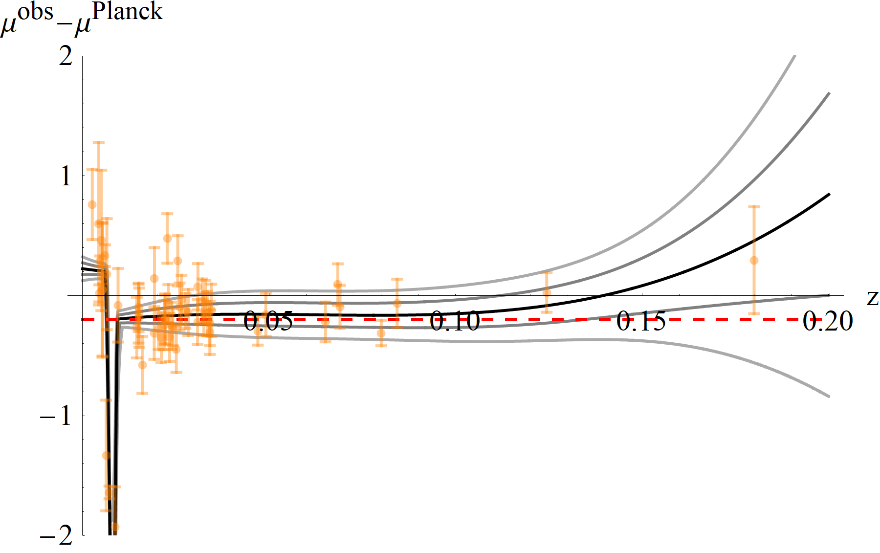
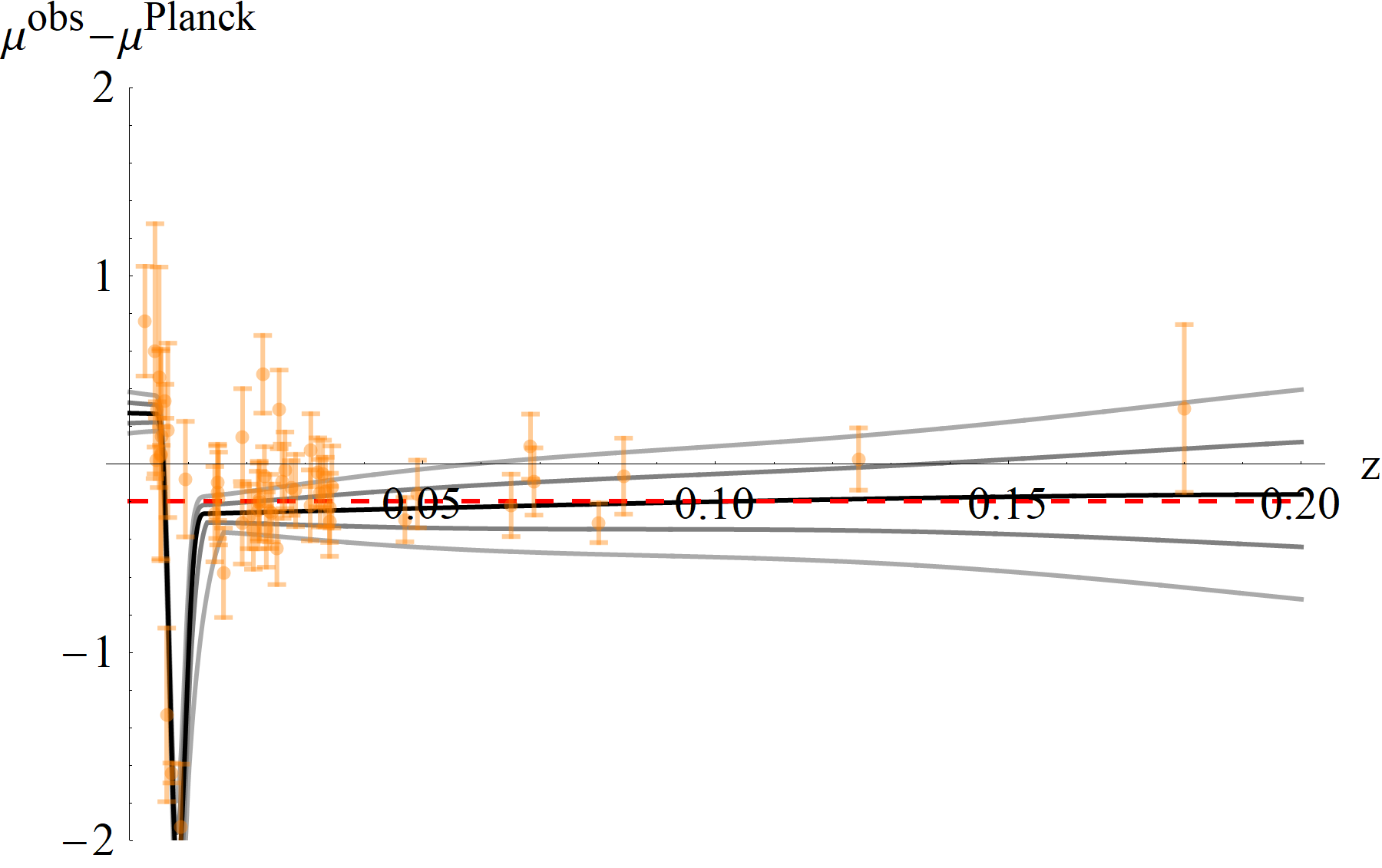
Figure 8: F3 standard candles distance modulus data (without peculiar velocity correction, with 250 ${\rm km\,s^{-1}}$ velocity dispersion for SNe, and without outlier removal) are plotted with their best fit (black), 68% (gray) and 95% (light gray) confidence bands according to the method of section 3, with $z_{\rm max}=0.2$ and a $(0,0,5)$ model on the left, $z_{\rm max}=0.4$ and a $(0,1,5)$ model on the right. The dashed red line is plotted as a reference and corresponds to $\mu^{\rm Riess}-\mu^{\rm Planck}$. In both cases the fits are not invertible.

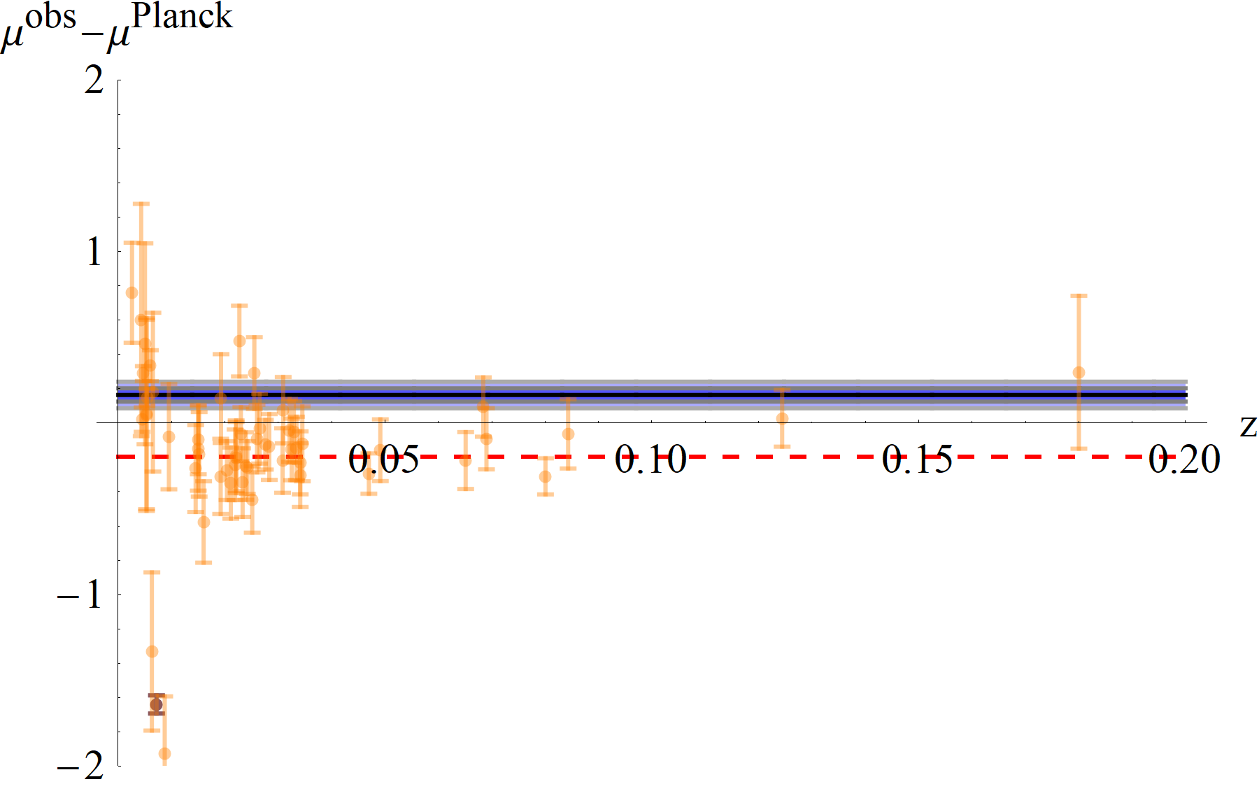
(a) NGC 4536 removed $(1,0,0)$

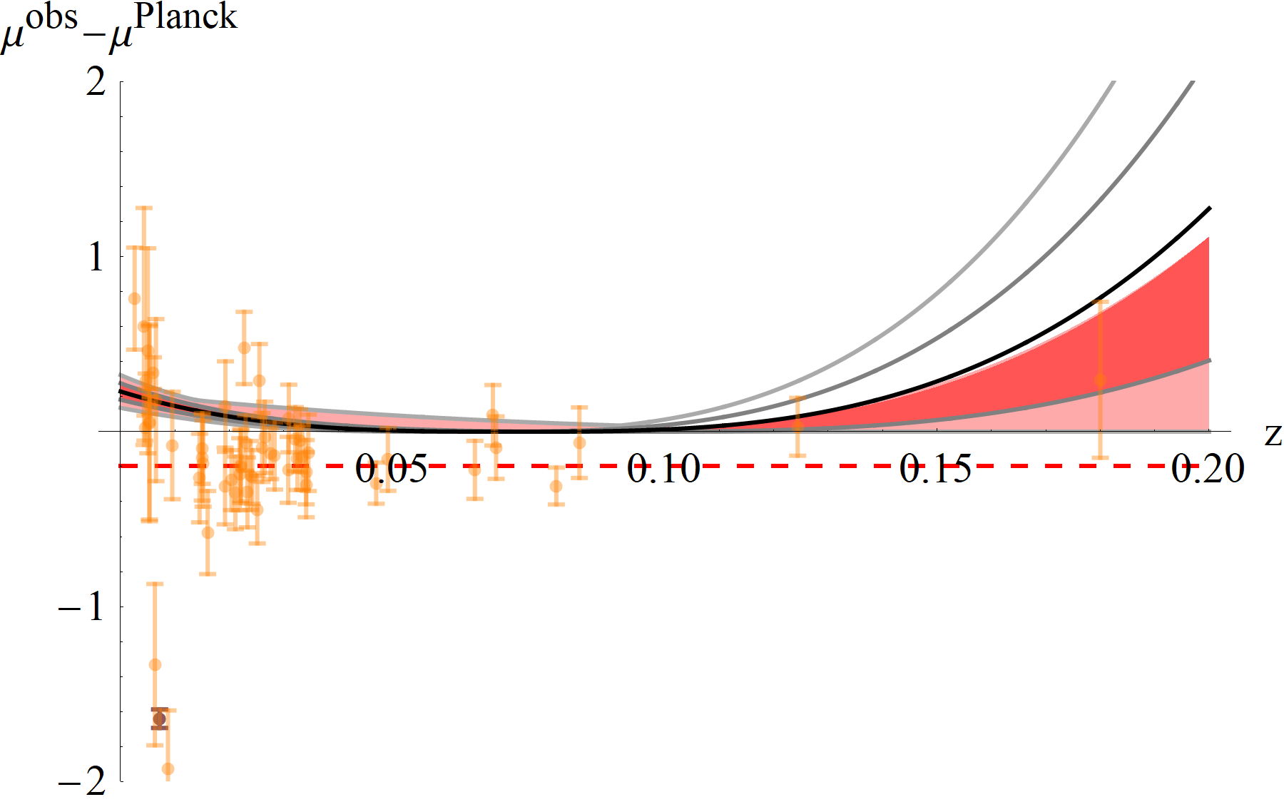
(b) NGC 4536 removed $(0,0,1)$

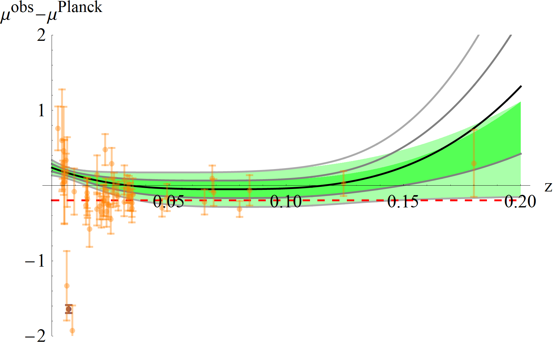
(c) NGC 4536 removed $\mathbf{(1,0,1)}$

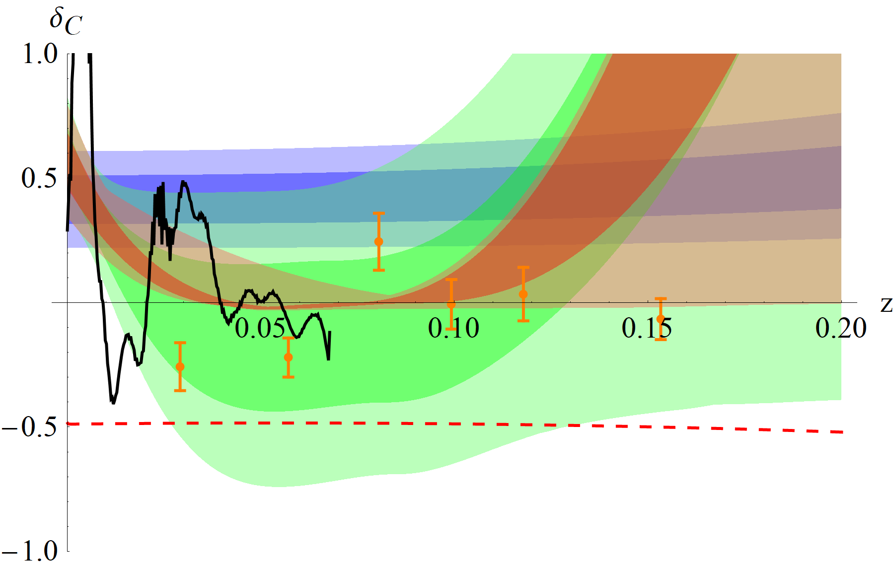
(d) Inverted density

Figure 9: Distance modulus best fit models are plotted for F3 with $z_{\rm max}=0.2$, without peculiar velocity corrections and with a 250 ${\rm km\,s^{-1}}$ velocity dispersion for SNe. The model parameters and the removed data points are shown in the sub-captions. (a, b, c): Standard candles distance modulus data are plotted with their best fit (black), 68% (gray) and 95% (light gray) confidence bands according to the method of section 3. The invertible bands are shown as the shaded region (68%-darker color, 95%-lighter color), while the removed outliers are shown as darker data points. The dashed red line is plotted as a reference and corresponds to $\mu^{\rm Riess}-\mu^{\rm Planck}$. Case (c) is preferred. (d): The confidence bands of the inverted density contrast corresponding to the invertible bands of the distance modulus are shown (68%-darker color, 95%-lighter color). The data points of $\mathcal{K}$13 are plotted in orange, the 2M++ density contrast averaged over F3 as a solid black curve, and the dashed red line is for density contrast that would lead to a local Hubble parameter $H_{0}^{\rm loc}=H_{0}^{\rm Riess}$ assuming a large scale $H_{0}^{LS}=H_{0}^{\rm Planck}$. The bands are color coded case by case with blue (a), red (b), green (c).

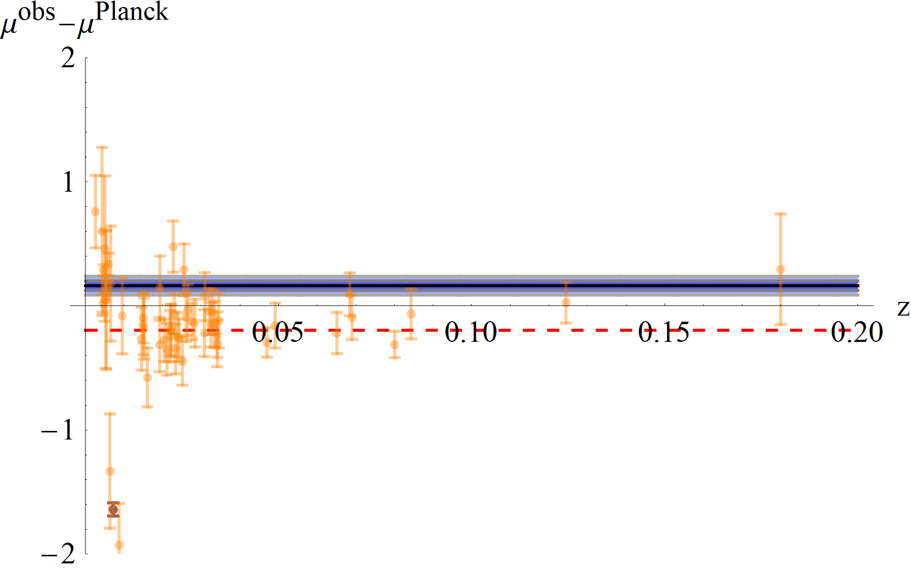
(a) NGC 4536 removed $(1,0,0)$

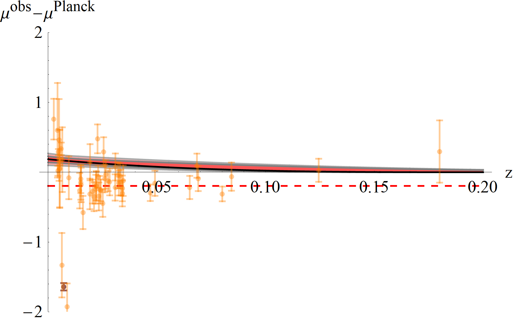
(b) NGC 4536 removed $(0,0,1)$

(c) NGC 4536 removed $\mathbf{(1,0,1)}$

(d) Inverted density

Figure 10: Distance modulus best fit models are plotted for F3 with $z_{\rm max}=0.4$, without peculiar velocity corrections and with a 250 ${\rm km\,s^{-1}}$ velocity dispersion for SNe. The model parameters and the removed data points are shown in the sub-captions. (a, b, c): Standard candles distance modulus data are plotted with their best fit (black), 68% (gray) and 95% (light gray) confidence bands according to the method of section 3. The invertible bands are shown as the shaded region (68%-darker color, 95%-lighter color), while the removed outliers are shown as darker data points. The dashed red line is plotted as a reference and corresponds to $\mu^{\rm Riess}-\mu^{\rm Planck}$. Case (c) is preferred. (d): The confidence bands of the inverted density contrast corresponding to the invertible bands of the distance modulus are shown (68%-darker color, 95%-lighter color). The data points of $\mathcal{K}$13 are plotted in orange, the 2M++ density contrast averaged over F3 as a solid black curve, and the dashed red line is for density contrast that would lead to a local Hubble parameter $H_{0}^{\rm loc}=H_{0}^{\rm Riess}$ assuming a large scale $H_{0}^{LS}=H_{0}^{\rm Planck}$. The bands are color coded case by case with blue (a), green (b), red (c).

7 Discussions

We here discuss the implications and the limitations of our study and describe some possible ways to increase its precision to further investigate the existence of inhomogeneities.

7.1 Peculiar velocity and galaxy surveys

The 2M++ catalogue [40] gives the density field and the predicted peculiar velocities within 200 ${\rm Mpc}/h$ ($z<0.67$). The under-density claimed by $\mathcal{K}$13 along F2 and F3 has a size of $\sim 300\,{\rm Mpc}/h_{70}$ ($z\sim 0.07$) and is thus roughly outside the 2M++ catalogue. Also the boundary of the under-density, i.e., an over-dense filament-like structure at $z\sim 0.08$ (Sloan Great Wall), is slightly outside the 2M++ window. If this “super void + filament” structure exists, the depth limitation of 2M++ does not allow a full reconstruction of the velocity field that takes the structure into consideration.

Another independent galaxy survey, Cosmicflows-2 of [68], suggests that we are part of a super-structure (basin of attraction) called “Laniakea”. As shown in figure 1 of [68], along the center of F3 (corresponding to the +Y direction in supergalactic coordinates) there seems to exist a large void which would confirm $\mathcal{K}$13’s finding, also in possible agreement with figure 9(c). In principle, such an inhomogeneity should be detectable in 2M++, Cosmicflows-2, and $\mathcal{K}$13. In practice though, it is hard to compare these surveys since for example $\mathcal{K}$13 only uses GAMA DR1 [69] as an anchor and does a comparison with its own analysis of the old 2M++ dataset [56], while [40] uses its own average density as the background. The different normalization introduces additional scaling to the density contrast that may jeopardize the whole comparison of their density contrasts. The under-density that we find in F3 is not aligned with the CMB dipole, and thus does not seem explainable from the bulk flow of the Local Group.

7.2 Choice of background and the associated background density

As discussed before, one plausible explanation for the discrepancy between the observed $H_{0}$ values of $\mathcal{R}$16 and $\rm Planck$ is that the assumed background density in 2M++, i.e. the averaged density within its observation depth, is not the real background density. If we take $\mathcal{K}$13 background density we would have to rescale the density contrast of 2M++ as

$$\delta_{C}^{\rm cor}=\frac{\tilde{\rho}_{\text{{2M++}}}}{\tilde{\rho}_{\text{$\mathcal{K}${13}}}}(1+\delta_{C})-1,$$ (7.1)

where $\delta_{C}^{\rm cor}$ is the rescaled density contrast, while $\tilde{\rho}_{\text{{2M++}}}$ and $\tilde{\rho}_{\text{$\mathcal{K}${13}}}$ are the assumed background density of 2M++ and $\mathcal{K}$13. According to $\mathcal{K}$13 the needed rescaling is a factor of $\sim 0.6$. As shown in figure 11 after the rescaling of the density contrast in both subregion F1 and F3 the 2M++ averaged density matches quite well with the inverted density that we obtain in section 6. This, along with the finding that the inverted density in F3 is compatible with the density in $\mathcal{K}$13, indicates that the existence of the $\sim 300$ Mpc inhomogeneity of $\mathcal{K}$13 could explain the tension between $\mathcal{R}$16 and $\rm Planck$ estimation of $H_{0}$.

Alternatively we may also assume a different background $H_{0}^{\text{$\mathcal{R}${16}}}=73.24$ ${\rm km\,s^{-1}\,{\rm Mpc}^{-1}}$. In that case all the inverted densities shown in section 6 need to be rescaled as (up to the zeroth order in redshift)

$$\delta_{C}^{\rm cor}\sim\frac{H_{0}^{\text{$\mathcal{R}${16}}}}{H_{0}^{\rm Planck}}(\frac{3}{f}+\delta_{C})-\frac{3}{f},$$ (7.2)

where $f\sim\Omega_{m0}^{0.55}$ is the growth rate, while $H_{0}^{\text{$\mathcal{R}${16}}}$ and $H_{0}^{\rm Planck}$ are the Hubble parameter of $\mathcal{R}$16 and $\rm Planck$. The resulting shift on the inverted density contrast is $\sim 0.5$, again consistent with the observed density contrast of 2M++.

Both explanations could explain simultaneously the luminosity distance data of standard candles and the luminous density data. However, a higher $H_{0}$ value would create inconsistencies with the CMB observations, and since there are solid theoretical reasons to expect that high redshift observations are insensitive to local structure [24], it seems more justified to interpret these results as the need for a proper renormalization of 2M++ rather than invoking an hypothetical early Universe physics modification which may affect CMB observations independently from local structure, as proposed for example in [70]. In any case, the difference in the reconstructed density profile for the two different directions is an evidence of anisotropy which cannot be explained by considering different values of $H_{0}$, and would remain even assuming $H_{0}^{\text{$\mathcal{R}${16}}}$.

(a) Subregion F1 $(1,0,0)$

(b) Subregion F3 $z_{\rm max}=0.2$ with NGC 4536 removed $(1,0,1)$

(c) Subregion F3 $z_{\rm max}=0.4$ with NGC 4536 removed $(1,0,1)$

Figure 11: The confidence bands of the inverted density contrast for the standard candles distance modulus data without peculiar velocity corrections and with a 250 ${\rm km\,s^{-1}}$ velocity dispersion for SNe are shown (68%-darker color, 95%-lighter color). The model parameters and the cuts of the dataset are shown in the sub-captions. In addition the data points of $\mathcal{K}$13 are plotted in orange for F3 and green for F1, the 2M++ density contrast averaged over the subregion specified in the sub-captions as a solid black curve, its rescaled version by a factor of $0.6$ according to $\mathcal{K}$13 as a dashed black curve, and the dashed red line is for density contrast that would lead to a local Hubble parameter $H_{0}^{\rm loc}=H_{0}^{\rm Riess}$ assuming a large scale $H_{0}^{LS}=H_{0}^{\rm Planck}$.

7.3 Impact of Supernovae data quality on the reconstruction of density

Our analysis uses 70 (145) SNe or Cepheids-hosting galaxies in F1 and 55 (60) in F3 for $z_{\rm max}=0.2$ ($z_{\rm max}=0.4$). Despite the seemingly “large” numbers for such a small redshift range, the redshift distribution of the data has some limitations. In F2 there are no SNe, while $\mathcal{K}$13 also reports an under-density profile in that field of view. Along F1 SNe are distributed evenly in redshift, but along F3 most of SNe and Cepheids-hosting galaxies are at $z<0.04$ (only 9 SNe between $0.04<z<0.2$ and only 5 SNe between $0.2<z<0.4$). So we may be missing the peak of $\mathcal{K}$13 if it exists. As our method consists in a 1-dimensional fit, SNe with the same redshift but different angles are fitted together, implying that some angular regions can have more weight than others if more SNe are located therein. This can explain the deviation of our reconstructed profiles with respect to the angular average of the 2M++ density profile. In addition, SNe are affected by intrinsic dispersion and, as shown in the past, their intrinsic color can play an important role in assessing the existence of a Hubble bubble (c.f. [71, 72, 73]).

Nevertheless we can still draw some conclusions from our results. First, according to figures 11(b) and 11(c), the inverted density contrasts could not reveal the over-dense regions of 2M++ very well, except at very small redshifts ($z\lesssim 0.02$). According to figure 3, all SNe actually lie in regions with density very close to the background, which shows that apparently the SNe sample does not probe well extreme density variations. We can argue that this phenomenon is due to the fact that, firstly the selected models are too simple to accommodate fine structures, secondly most star-forming galaxies are lower-mass galaxies outside the densest regions. According to [74] the cutoff scale for SNe-producing galaxy mass is $10^{11}M_{\astrosun}$. Therefore, qualitatively SNe underestimate the small scale density fluctuations and that makes SNe more suitable for probing density fluctuations on large scales compared to galaxies.

7.4 Statistical significance of the fits

There are recent publications (c.f. [4, 43, 41]) using model-independent techniques like Gaussian process or the Bayesian hyper-parameters method to fit data. Since the multiple models we have are selected using step-wise regression and ranked using $\chi^{2}$, it would be interesting to consider those methods as well.

In order to test the statistical significance of our results, we ran 10000 Monte Carlo simulations assuming a homogeneous universe with $\rm Planck$ cosmological parameters, with each simulation having the same number of data points as in F3, randomly generated with the same errors of the observational data in F3.

Using a stepwise regression method with a 95% F-test Threshold we found that is 99.5% of the best fit models are homogeneous (either a $(0,0,0)$ or a $(1,0,0)$ model). Given the low 0.5% misidentification rate, the selection of an inhomogeneous model as the best fit model is unlikely to be a statistical fluke. In addition, we may also consider the full 3-$D$ fit of the luminosity distance by extending our fitting method to a multi-dimensional version. In that case we may apply a density map reconstruction technique to recover the full-sky density map, and compare it directly to galaxy surveys like 2M++ and Cosmicflows-2, without depending on window averaging. Notice that ”outliers” removal may be an artifact due to window averaging. For example, NGC 4536, 2006x and 1999cl are right behind the Virgo cluster and NGC 4424 is in front of it, making them prone to the extreme density fluctuations within the Virgo cluster. These four objects in fact happen to be most frequently selected as outliers in our analysis.

8 Conclusions

We have applied a new method to extract information about the large scale structure from the observed distance modulus of supernovae (SNe) and Cepheids. We used a combination of the Union 2.1 Type Ia SNe of [45] (with an added 250 ${\rm km\,s^{-1}}$ velocity dispersion) and the Cepheid calibrators of [2] ($\mathcal{R}$16). The inversion method we utilize requires the input luminosity distance as a smooth function of the redshift, so we fit the observational data with a set of radial basis functions (RBFs), without any prior on the local structure (except for meta-fitting parameters such as the explicit form of RBF). Using this method, any deviation of the observed luminosity distance from its homogeneous Universe ($\Lambda$CDM) prediction can be used to reconstruct the local structure. Rather than fitting the complete dataset with SNe from the whole sky, we have analyzed the density profile along different directions. Under the assumption that lensing effects at low redshift are negligible the radial profiles in different angular directions have been modeled as independent LTB radial profiles.

Note that there is no fine tuning of the position of the observer since we are reconstructing the radial density profile in different directions separately. In other words, we are not assuming isotropy and the center of the coordinate system where the observer is located is not a center of spherical symmetry. The density profile in a given direction is a function of the radial coordinate and as such can be mapped into the geometry of a solution depending on a single function of the radial coordinate such as the LTB, since this is a one dimensional problem. Assuming the lensing effects are negligible at low redshift should be a good approximation. In other words the use of a LTB solution is just a computational tool and we are not assuming a spherically symmetric model of the local Universe, since we reconstruct radial profiles in different directions independently.

We focused on further investigating the existence of inhomogeneities with a size of several hundred ${\rm Mpc}$, which was previously studied by [39] ($\mathcal{K}$13) using observed luminosity density in different fields of observations. $\mathcal{K}$13 studied three different regions (which we call F1, F2, F3), while we reconstruct the density profile only in F1 and F3, where the number of SNe is high enough to allow a statistical analysis.

Our results are in good agreement with the rescaling of 2M++ proposed by $\mathcal{K}$13 for both F1 and F3. The agreement of our reconstructed density profiles for F3 is also good with respect to $\mathcal{K}$13, while in F1 at higher redshift there is some difference . The density profile along F1 and F3 directions are different and this clearly shows the existence of an anisotropy not detectable by 2M++.

The inhomogeneity detection depends crucially on the velocity dispersion of Cepheids-hosting galaxies. This is naturally expected since large values of the velocity dispersion can introduce noise in the data which dominate over the effects of inhomogeneities. As a confirmation of the importance of the velocity dispersion, we find that the very low-redshift peak in 2M++, corresponding to the Virgo cluster, is well reconstructed from the luminosity distance data when we consider a small velocity dispersion for Cepheids-hosting galaxies, but disappears for larger dispersion. This suggests that the Cepheids-hosting galaxies data should be analyzed assuming a value for the velocity dispersion smaller than the one used in $\mathcal{R}$16, and is supported by the observations of nearby clusters [54, 55]. Large values of the velocity dispersion could introduce an artificially strong noise in the analysis that contaminates the real signal of large scale structures on the velocity field.

According to our analysis, in some directions the size of the inhomogeneity is larger than the depth of the 2M++ survey. Consequently, the normalization of the latter with respect to the average density of the Universe may require a rescaling, which we find to be very close to what $\mathcal{K}$13 obtained. This could in fact play a very important role in explaining the apparent discrepancy between the local and large scale estimation of $H_{0}$ [24], due to the fact that about 40% of low redshift SNe used to estimate $H_{0}^{loc}$ are affected by the inhomogeneities we found along F1 and F3. In the future this method could be used to correctly normalize density maps with respect to the average density of the Universe, a procedure which can be especially important when galaxy catalogues have a depth smaller than the size of the large scale structure inside which they are embedded, as it seems the case for 2M++.

We also checked that our method does not depend significantly on meta-parameters. The accuracy of our distance-modulus fitting is obviously limited by the SNe data precision, and a higher number of events would reduce the size of the confidence bands. The inversion and the comparison with the luminosity density profiles are also limited by the non-uniform angular and redshift distribution of SNe. For instance, F3 does not have a lot of data points at $z\sim 0.08$ (with less than ten SNe for $0.04<z<0.2$), so the size of the inhomogeneity cannot be precisely confirmed. Future data could overcome these statistical limitations.

Our analysis could be extended to a larger dataset, for example the carefully calibrated SNe data presented in $\mathcal{R}$16 (see also [75, 76, 77] for SNe) and the density field of Cosmicflows [78]. We could also use the Nearby Supernova Factory data of [79] (see [80] for example) or other future surveys such as WFIRST, in order to find out whether or not we can reconstruct a more accurate large scale structure map and compare it to what is obtained using galaxy catalogues. Once new data will be available supernovae could become a very important source of information about large scale structure, especially useful at high redshift where other astrophysical objects are difficult to observe, allowing to overcome the limits of depth and angular limitation of galaxy catalogues. In the future it could be also interesting to develop a fully non linear inversion method which could be applied when the assumptions we made are not satisfied, such as at high red-shift, or when lensing is important.

Appendix A Effect of cosmological constant on density contrast

As briefly explained in the section 3.2, the effect of the cosmological constant on the density contrast is non-negligible at the very small redshift because the growth rate can play an important role despite the effects of dark energy on the luminosity distance are not important. Here we derive the effects of $\Lambda$ on $\delta_{C}$ comparing with perturbation theory. We then test the inversion method applying it to luminosity distance computed numerically using a $\Lambda$LTB solution showing that the reconstructed density contrast defined in eq. (3.22) is in good agreement with the numerical computation of the corresponding density profile.

According to [24], assuming a spherically symmetric universe, the density contrast $\delta_{C}$ in the pertubative regime is given by

$$\delta_{C} =\frac{\chi}{3}\frac{d\bar{\delta}}{d\chi}+\bar{\delta}\quad,\quad\bar{\delta}=\frac{3}{f}\left(\frac{D_{L}^{\rm obs}}{\overline{D}_{L}}-1\right)\left(1-z\right)^{-1}\,,$$ (A.1)

where $\chi$ is the unperturbed comoving distance, f the growth rate defined in eq. (3.23), $z$ the observed redshift at $\chi$, $D_{L}^{\rm obs}$ the observed and $\overline{D}_{L}$ the background luminosity distances at $z$, and $\bar{\delta}$ is the comoving-volume-averaged density contrast $\bar{\delta}=\left(4\pi\chi^{3}/3\right)^{-1}\int^{\chi}4\pi{\chi^{\prime}}^{2}\delta_{C}\left(\chi^{\prime}\right)d\chi^{\prime}$. For a ($\Lambda$)CDM model with a spherically symmetric density contrast perturbatively solved up to the first order, i.e. a linearized ($\Lambda$)LTB model, and cosmological background parameters estimated from large scale observations, the density contrast at first order in z can be expressed as

$$\delta_{C}^{\Lambda\rm LTB}(\Delta) =\frac{3}{f}\Delta+\frac{z}{f}\left(\frac{d\Delta}{dz}+4\Delta\right)\,,$$ (A.2)

$$\delta_{C}^{\rm LTB}(\Delta) =3\Delta+z\left(\frac{d\Delta}{dz}+4\Delta+3\Omega_{\Lambda 0}\left(1+\Delta\right)\right)\,,$$ (A.3)

where $\Delta=\frac{D_{L}^{\rm obs}}{D_{L}^{\text{Hom}}}-1\equiv 10^{\left(\mu^{obs}-\mu^{\text{Hom}}\right)/5}-1$ is the relative difference between observed luminosity distance and the luminosity distance $D_{L}^{\text{Hom}}$ of a homogeneous $\Lambda$CDM model with cosmological background parameters estimated from large scale observations, such as $\rm Planck$.

There are two differences between LTB and $\Lambda$LTB models. First, there are additional terms proportional to $\Omega_{\Lambda 0}$ in $\delta_{C}^{\rm LTB}$ coming from $D_{L}^{\text{Hom}}$. Second, the differences in the evolution of the Hubble flow and of the background matter density imply a different growth rate values. The density contrast we propose in eq. (3.22)

$$\delta_{C} =f^{-1}\left(\frac{\rho_{\rm inv}\left(D_{L}^{obs},z\right)}{\rho_{\rm inv}\left(D_{L}^{\rm Planck},z\right)}-1\right)\approx f^{-1}\left(\frac{1+\delta_{C}^{\text{LTB}}\left(\Delta\right)}{1+\delta_{C}^{\text{LTB}}\left(0\right)}-1\right)$$

$$\approx f^{-1}\left(3\Delta+z\left(\frac{d\Delta}{dz}+4\Delta-6\Omega_{\Lambda 0}\Delta\right)\right)\approx\left(1-2\Omega_{\Lambda 0}z\right)\delta_{C}^{\Lambda\text{LTB}}(\Delta)\,,$$ (A.4)

takes care of all the factors mentioned above, and is approximately the density contrast in a $\Lambda$LTB model up to first order in redshift. The term $-2\Omega_{\Lambda 0}z\delta_{C}^{\Lambda\text{LTB}}(\Delta)$ is actually at the second order and we do not consider it for simplicity.

To test the validity of eq. (3.22), we consider a specific setup (compensated void, i.e. $\lim_{z\to\inf}\bar{\delta}\to 0$) presented in [27]. As shown in fig.  12, the reconstructed density contrast obtained using eq. (3.22) is in very good agreement with the numerical calculation using the $\Lambda$LTB solution, indicating that eq. (3.22) is indeed a good approximation.

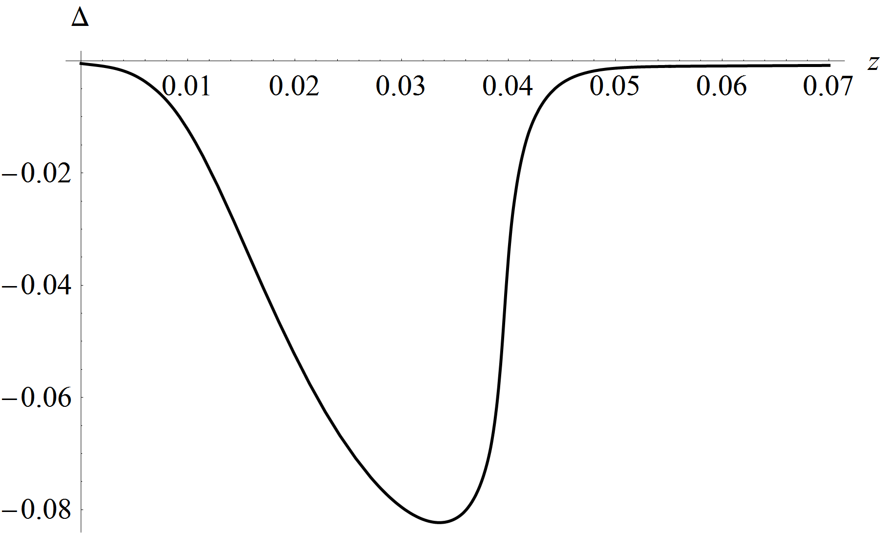
Figure 12: Left: The plot of $\Delta=\frac{D_{L}}{D_{L}^{\rm Planck}}-1$ for the model from [27]. Right: The plot of density contrast for the model from [27]. The black curve is the original density contrast of the $\Lambda$LTB model. The grey curve is the density profile reconstructed from the luminosity distance of the $\Lambda$LTB model using the linear method defined in eq. (A.1). The dashed curve is the density profile reconstructed using the non linear method defined in eq. (3.22). The profile reconstructed using the non linear method matches well the original profile, while the pertubative formula is not as accurate in some regions due to non linear effects.

Nevertheless there are some limitations related to the inversion derived above, since it is based on the low red-shift expansion of eq. (A.1). The first limitation is related to the fact that at high red-shift eq. (3.22) may require higher order corrections in the red-shift expansion. The second has to do with the fact that eq. (3.22) is assuming that the Doppler effect is the dominant contribution, but in the fully non linear regime it is possible that other contributions such as lensing or ISW could become important. Consequently from a purely mathematical point of view it cannot be claimed that the inversion method in eq. (3.22) is fully non linear, but it can at least be stated that is better than the perturbative method as shown in fig. 12, and quite accurate as long as the Doppler term is dominating, which is a reasonable assumption at low red-shift.

As explained in appendix B lensing observations support the assumption that the Laplacian of the gravitational potential in the directions orthogonal to the line of sight is negligible compared to the Laplacian in the radial direction, so when applied to low red-shift data, the method should be accurate, but from a purely mathematical point of view it will be less accurate when applied to high red-shift data, or for systems with large shear or large non Doppler effects.

Appendix B LTB inversion and anisotropic matter distributions

To justify the application of LTB inversion method we will demonstrate that up to first order in perturbation theory and assuming, as supported by observations[59, 60, 61, 62, 63, 64], a negligible lensing effect, it is possible to express the effects of inhomogeneities on the luminosity distance only in terms of $\delta_{C}$ along the line of sight. According to eq. (B1) of [66], the luminosity distance can be expressed as

$$d_{L}\left(z_{S},\vec{n}\right) =\left(1+z_{S}\right)\Delta\eta\Bigg{\{}1+\frac{\Psi_{O}-\Psi_{S}-\left(\vec{v}_{O}-\vec{v}_{S}\right)\cdot\vec{n}}{\mathcal{H}_{S}\Delta\eta}-\Psi_{S}-\vec{v}_{S}\cdot\vec{n}$$

$$+\int_{\eta_{S}}^{\eta_{O}}d\eta\left[\frac{2}{\Delta\eta}-\frac{2}{\Delta\eta}\left(\frac{1}{\mathcal{H}_{S}}-\int_{\eta_{S}}^{\eta}d\eta^{\prime}\right)\nabla_{\vec{n}}-\frac{\left(\eta-\eta_{S}\right)\left(\eta_{O}-\eta\right)}{\Delta\eta}\nabla_{\bot}^{2}\right]\Psi\Bigg{\}}\,,$$ (B.1)

where subscripts _O and _S stand for observer and source, $\nabla_{\bot}^{2}\equiv\triangle-\nabla_{\vec{n}}\nabla_{\vec{n}}+2\left(\eta_{O}-\eta\right)^{-1}\nabla_{\vec{n}}$ is the screen-space Laplacian[58], $A\cdot B=A^{i}B_{i}$ is the inner product with $i$ the spatial index running from $1$ to $3$, $\nabla_{\vec{n}}=\vec{n}\cdot\vec{\nabla}$ is the covariant derivative along $\vec{n}$ , $\triangle=\vec{\nabla}\cdot\vec{\nabla}$ is the 3-Laplacian, $\vec{v}$ is the peculiar velocity, $\vec{n}$ is the unit 3-vector along the photon direction, $\eta$ is the conformal time along the photon trajectory, $\Delta\eta\equiv\eta_{O}-\eta_{S}$, $\Psi$ is the gravitational potential, and $\mathcal{H}$ is the conformal Hubble parameter. Only the second derivative term explicitly depends on quantities off the line of sight, and corresponds to the convergence in the context of the weak lensing[58, 63], which at low red-shift should be negligible, as supported both by theoretical calculations [58] and observation [59, 60, 61, 62, 63, 64].

Assuming $\nabla_{\bot}^{2}\Psi\approx 0$, zero pressure for the background and perturbations, and that the peculiar velocity field is irrotational, the perturbed Einstein’s equations give [81]

$$\frac{2}{3}\Omega_{M}\mathcal{H}^{2}\delta_{C}=\triangle\Psi=\nabla_{\bot}^{2}\Psi+n^{i}\nabla_{i}\left(n^{j}\nabla_{j}\Psi\right)-2\left(\eta_{O}-\eta\right)^{-1}n^{i}\nabla_{i}\Psi\approx r^{-2}\partial_{r}\left(r^{2}\partial_{r}\Psi\right)\,,$$ (B.2)

$$\frac{2}{3}\Omega_{M}\mathcal{H}^{2}n^{i}v_{i}=-n^{i}\partial_{i}\left[\left(\partial_{\eta}+\mathcal{H}\right)\Psi\right]\equiv\left(\partial_{\eta}+\mathcal{H}\right)\partial_{r}\Psi=f\mathcal{H}\partial_{r}\Psi\,,$$ (B.3)

where $\Omega_{M}$ is the matter density parameter, $r\equiv\eta_{O}-\eta$ the comoving distance from the observer, $\partial_{r}=-n^{i}\partial_{i}$ the partial derivative of $r$, $\partial_{\eta}$ the conformal time derivative, $a$ is the scale factor, and $f$ is the growth rate defined in eq. (3.23). We will show later that lensing observations indeed support the assumption $\nabla_{\bot}^{2}\Psi\approx 0$. In a fully non linear regime this approximation may not be valid anymore, and a non spherically symmetric approach should be adopted. Nevertheless based on our analysis we expect the non linear effects to be negligible at low red-shift, as supported also by other observations [59, 60, 63].

It is important to check under which conditions the orthogonal part of the Laplacian $\nabla_{\bot}^{2}\Psi$ can be neglected, and this can be done by using its relation to the the convergence

$$\kappa\left[\eta_{S}\right]\equiv-\int_{\eta_{S}}^{\eta_{O}}d\eta\frac{\left(\eta_{O}-\eta\right)\left(\eta-\eta_{S}\right)}{\Delta\eta}\nabla_{\bot}^{2}\Psi\,.$$ (B.4)

Solving eq. (B.2) without assuming $\nabla_{\bot}^{2}\Psi\approx 0$, we obtain

$$\Psi=\Psi_{O}+\int r^{-2}dr\int r^{\prime 2}dr^{\prime}(\triangle\Psi-\nabla_{\bot}^{2}\Psi)\approx\Psi_{\text{iso}}+\kappa\,,$$ (B.5)

where $r$ is the comoving distance from the observer, $\Psi_{\text{iso}}$ is the potential obtained assuming isotropy, i.e. the solution of $r^{-2}\partial_{r}\left(r^{2}\partial_{r}\Psi_{ISO}\right)=\frac{2}{3}\Omega_{M}\mathcal{H}^{2}\delta_{C}$.

From the identity $\frac{d}{d\eta}\Psi\left(\eta,\vec{x}\left(\eta\right)\right)=\frac{\partial}{\partial\eta}\Psi+\nabla_{\vec{n}}\Psi\equiv s^{-1}\Psi+\nabla_{\vec{n}}\Psi$, we have

$$\int_{\eta_{S}}^{\eta_{O}}d\eta\frac{\Psi}{s}=\Psi\bigg{|}_{\eta_{S}}^{\eta_{O}}- \int_{\eta_{S}}^{\eta_{O}}d\eta\nabla_{\vec{n}}\Psi\sim\left(\Psi-s\nabla_{\vec{n}}\Psi\right)\bigg{|}_{\eta_{S}}^{\eta_{O}}-s\int_{\eta_{S}}^{\eta_{O}}d\eta\nabla_{\bot}^{2}\Psi\,,$$ (B.6)

$$\int_{\eta_{S}}^{\eta_{O}}d\eta\frac{\nabla_{\vec{n}}\Psi}{s}\sim \nabla_{\vec{n}}\Psi\bigg{|}_{\eta_{S}}^{\eta_{O}}+\int_{\eta_{S}}^{\eta_{O}}d\eta\nabla_{\bot}^{2}\Psi\,,$$ (B.7)

$$\int_{\eta_{S}}^{\eta_{O}}d\eta\int_{\eta_{S}}^{\eta}d\eta^{\prime}\frac{\nabla_{\vec{n}}\Psi}{s}= -\Delta\eta{\nabla_{\vec{n}}\Psi}_{S}+\int_{\eta_{S}}^{\eta_{O}}d\eta\left(1-\int_{\eta_{S}}^{\eta}d\eta^{\prime}\nabla_{\vec{n}}\right)\nabla_{\vec{n}}\Psi$$

$$\sim s\nabla_{\vec{n}}\Psi\bigg{|}_{\eta_{S}}^{\eta_{O}} -\Delta\eta{\nabla_{\vec{n}}\Psi}_{S}+\int_{\eta_{S}}^{\eta_{O}}d\eta\left(s+\int_{\eta_{S}}^{\eta}d\eta^{\prime}\right)\nabla_{\bot}^{2}\Psi\,,$$ (B.8)

where $\sim$ denotes that terms depending only on the density contrast $\delta_{C}$ along the line of sight, are dropped and we have defined $s^{-1}=\left(f-1\right)\mathcal{H}$, and approximated it as a constant, which should be reasonable within the regime of interest ($z<0.2$).

According to eq. (B.1) the relative fractional difference between the perturbed and background luminosity distance can be split into the sum of a radial $\Delta_{r}$ and transverse $\Delta_{\bot}$ part as

$$\frac{d_{L}\left(z_{S},\vec{n}\right)}{\left(1+z_{S}\right)\Delta\eta}-1 =\Delta_{r}+\Delta_{\bot}=\Delta_{r}-\frac{1}{\Delta\eta}\int_{\eta_{S}}^{\eta_{O}}d\eta\left[\frac{2s}{\mathcal{H}_{S}}+\int_{\eta_{S}}^{\eta}d\eta^{\prime}\left(\eta^{\prime}-\eta_{S}-2s\right)\right]\nabla_{\bot}^{2}\Psi\,.$$ (B.9)

The first part $\Delta_{r}$ contains terms depending only on observables along the line of sight. The term $\Delta_{\bot}$ is associated to the transverse part of the Laplacian, it is the one which is being neglected when assuming isotropy, and as such can be interpreted as the error due to such an approximation. Using eq. (B.4) we can conveniently write $\Delta_{\bot}$ in terms of the convergence as

$$\Delta_{\bot} =\frac{2s}{\mathcal{H}_{S}}\left(\frac{\kappa^{\prime}}{\Delta\eta}-2\mathbf{E}\left[\frac{\kappa^{\prime}}{\eta_{O}-\eta}\right]\right)+2s\left(\kappa^{\prime}-\mathbf{E}\left[\kappa^{\prime}\right]\right)+\kappa\,,$$ (B.10)

where $\kappa^{\prime}\left[\eta\right]=\frac{\partial}{\partial\eta}\kappa\left[\eta\right]$ and $\mathbf{E}\left[F\right]=\frac{1}{\Delta\eta}\int_{\eta_{S}}^{\eta_{O}}d\eta F$.

Given that the shear power spectrum $P_{\gamma}$ is the same as the convergence power spectrum $P_{\kappa}$ (c.f. e.g. eq. (30) of [63]), we may estimate the error due to assuming isotropic by using weak lensing observations. According to [59, 60, 61, 62, 63, 64] lensing observations give a value of the shear power spectrum of $\sim 10^{-4}z^{2}$, implying that the error in neglecting $\Delta_{\bot}$ is indeed negligible for any practical application of the inversion method. Furthermore the convergence power spectrum is theoretically predicted [82] to grow as $z_{S}^{1.5}\sim z_{S}^{2.5}$, which implies that the dominating part of $\Delta_{\bot}$ decays approximately as $1/\Delta\eta$, confirming the validity of the isotropic approximation in the linear regime.

Appendix C Results with an additional dispersion added to Cepheids-hosting galaxies

We present here the results of our analysis in F1 and F3, without peculiar velocity corrections, and as opposed to section 6, with $v_{c}=40$. The results are very similar to the case excluding this dispersion, but are still differing slightly due to the induced small decrease of Cepheids importance (higher uncertainty).

For F1, where most high redshift SNe are located, without removing any outlier and with redshift cut $z_{\rm max}=0.2$, the fit we get is almost identical to figure 7, with either a $(1,0,0)$ model with $H_{0}^{\rm loc}=74.18\pm 1.89$ ${\rm km\,s^{-1}\,{\rm Mpc}^{-1}}$ for a F-test Threshold $>38\%$, or a inhomogeneous $(1,1,9)$ model when the F-test Threshold is lower. The reduced chi square $\chi_{R}^{2}\sim 0.74$ of the inhomogeneous model is not so much lower than that of the $(1,0,0)$ model ($\chi_{R}^{2}\sim 1.01$).

For F3, without outliers removal, a $(0,0,5)$ model with both $z_{\rm max}=0.2$ and $z_{\rm max}=0.4$ cases is preferred. Again the fits are very similar to what we obtain in section 6. Other fits are presented in table 4 and are very similar to those presented in table 3.

Finally one can observe that the different fits for $z_{\rm max}=0.2$ and $z_{\rm max}=0.4$, presented in figure 13, are very similar to those obtained in figures 9 and 10, and the conclusions made in section 6 regarding $\mathcal{K}$13 and 2M++ still hold.

$z_{\rm max}$	Fig.	$\chi_{R}^{2}$	Threshold (%)	PRESS	Param.	Removal
0.2	N/A	11.9	Not Preferred	982.9	$76.22\pm 3.87$
	N/A	1.25	$25\sim 100$	166.2	$(0,0,5)$
	N/A	2.15	$97.6\sim 100$	116.1	$(0,0,0)$	NGC 4536
	13(a)	1.99	$95.0\sim 97.5$	111.5	$63.37\pm 1.50$
	N/A	1.88	$73\sim 94.9$	109.0	$(0,0,1)$
	N/A	1.65	$99.2\sim 100$	87.3	$(0,0,0)$	+ 1999cl
	N/A	1.30	$74\sim 99.1$	76.6	$(0,0,1)$
	13(b)	1.29	Not Preferred	83.3	$(1,0,1)$
0.4	N/A	11.0	$97.6\sim 99.0$	988.8	$76.23\pm 3.72$
	N/A	2.46	$15\sim 97.5$	662.5	$(0,0,5)$
	N/A	2.08	$97.7\sim 100$	122.8	$(0,0,0)$	NGC 4536
	N/A	1.94	$69\sim 97.6$	118.5	$63.40\pm 1.47$
	13(c)	1.97	Not Preferred	126.8	$(1,0,1)$
	N/A	1.47	$88\sim 99.1$	89.0	$63.32\pm 1.28$	+ 1999cl
	N/A	1.43	$61\sim 87$	92.1	$(0,0,1)$

Table 4: Distance modulus best fit model parameters with progressive removal of the outliers for F3, without peculiar velocity correction, with $v_{c}=40$, and with 250 ${\rm km\,s^{-1}}$ velocity dispersion for SNe. The Threshold column shows the F-test threshold of the model.

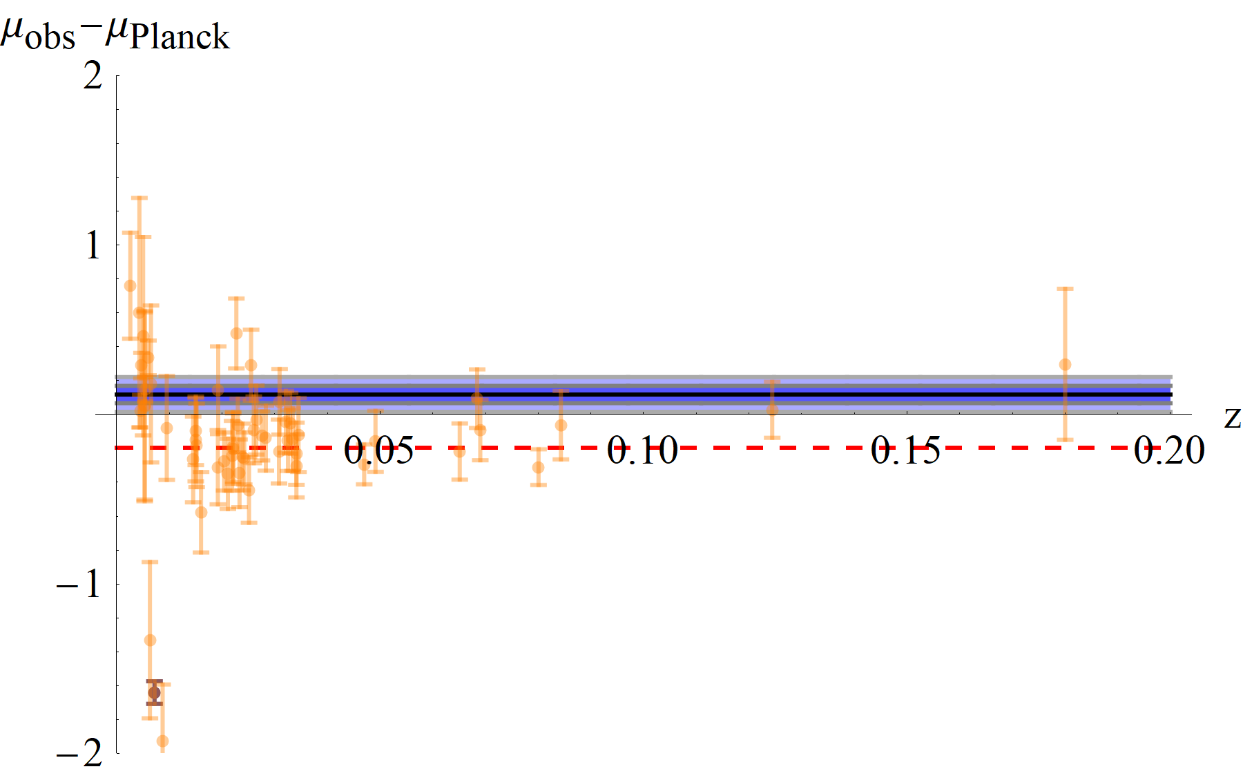
(a) $z_{\rm max}=0.2$ NGC4536 removed $(1,0,0)$

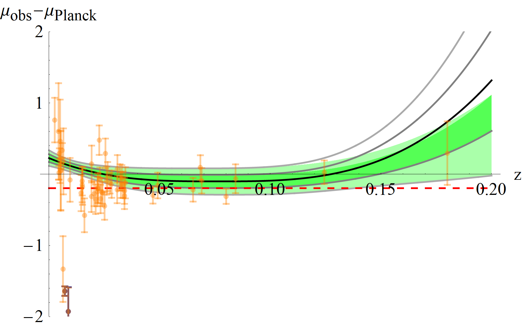
(b) $z_{\rm max}=0.2$ NGC4536 and 1999cl removed $(1,0,1)$

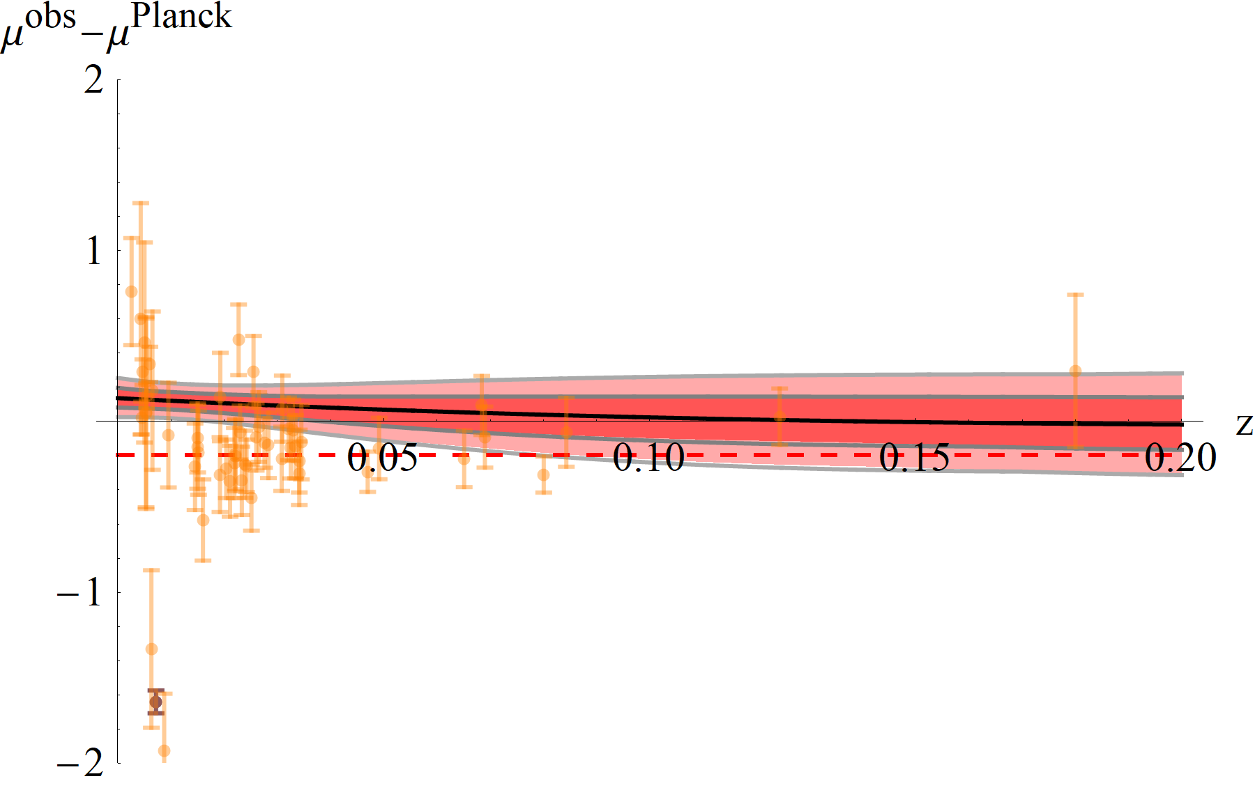
(c) $z_{\rm max}=0.4$ NGC4536 removed $(1,0,1)$

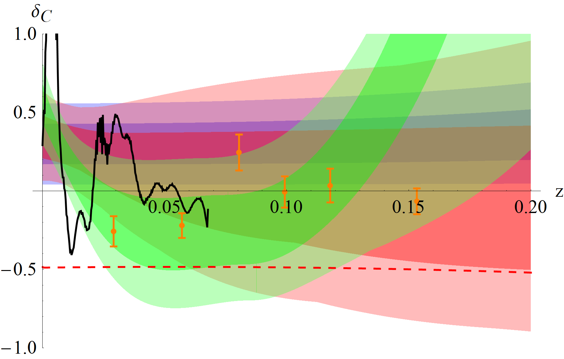
(d) Inverted density

Figure 13: Distance modulus best fit models are plotted for F3 without peculiar velocity corrections and with $v_{c}=40$ ${\rm km\,s^{-1}}$. The redshift cut $z_{\rm max}$, model parameters and the removed data points are shown in the sub-captions. (a, b, c): Standard candles distance modulus data are plotted with their best fit (black), 68% (gray) and 95% (light gray) confidence bands according to the method of section 3. The invertible bands are shown as the shaded region (68%-darker color, 95%-lighter color), while the removed outliers are shown as darker data points. The dashed red line is plotted as a reference and corresponds to $\mu^{\rm Riess}-\mu^{\rm Planck}$. (d): The confidence bands of the inverted density contrast corresponding to the invertible bands of the distance modulus are shown (68%-darker color, 95%-lighter color). The data points of $\mathcal{K}$13 are plotted in orange, the 2M++ density contrast averaged over F3 as a solid black curve, and the dashed red line is for density contrast that would lead to a local Hubble parameter $H_{0}^{\rm loc}=H_{0}^{\rm Riess}$ assuming a large scale $H_{0}^{LS}=H_{0}^{\rm Planck}$. The bands are color coded case by case with blue (a), green (b), red (c).

Appendix D Union2.1 + Riess et al. 2016 Cepheids dataset

We present here tables containing the data described in section 2 and on which our methodology of section 3 is applied. In table 5 are presented the Cepheid calibrators of [2] with their associated SNe. Several quantities such as the angular position and redshifts are extracted from external sources: Union 2.1, Ned and Simbad. Among the 3 fields, there are 8 SNe related to a Cepheid host-galaxy, among which 3 of them have redshift and magnitude recorded in Union 2.1 (2007af, 1994ae and 1995al, indicated by $\ast$ in tables 8 and 9) and 5 others for which redshift and magnitude are only given from the Cepheids (2009ig, 1981B, 1990N, 2012cg and 2012ht, indicated by $\dagger$ in table 5), i.e. SNe which are not in Union 2.1. We already explained in section 2.1 how the distance moduli are obtained. The ICRS sky positions are written in degrees and the magnitude $\mu$, plus its error $\Delta\mu$ before adding the calibration error, are presented. For types, the letters denote the following: ‘o’ indicates the so-called outliers in Union 2.1, ‘z’ is for redshifts $<0.015$ and ‘h’ for redshifts $>0.2$ and $\leq 0.4$; $\ast$ and $\dagger$ were explained above. Finally, we present in tables 6-7, 8 and 9 the respective Union 2.1 SNe of [45] and used in fields F1, F2 and F3. Angular positions are extracted from Simbad, and given with 3 digits of precision. redshifts $z$ are from Union 2.1 and shown with 5 digits (when available). $(\mu,\Delta\mu)$ are also from Union 2.1 and $\Delta\mu^{250}$ is computed with the additional 250 ${\rm km\,s^{-1}}$ velocity dispersion. They are shown with only 4 digits of precision.

Table 5: Cepheids-hosting galaxies of [2] with additional data. The Cepheid-hosting galaxy name and the name of the hosted SN are from [2]. Angular positions of host galaxies are from Simbad, in ICRS decimal format. Values of $(\mu,\Delta\mu)$ come from [2], while $\Delta\mu^{250}$ refers to the modified distance modulus error after considering an additional velocity dispersion of 250 ${\rm km\,s^{-1}}$ to the hosted SN redshift $z_{\rm SN}$, but before adding the calibration error. Values $z$(NED) are the host redshifts taken from Ned and $z_{\rm SN}$ are from Union 2.1, Simbad, or Extragalactic Distance Database (Edd) from [83] depending on availability. For some cases (denoted by “/”) none of these 3 sources have redshifts. NGC 4258 does not host a SN. Angles are truncated to 3 digits, similarly for $\Delta\mu^{250}$ and $\Delta\mu$ (except when Union 2.1 does not reach this precision).

Cepheid	Co-hosted	R.A.	Dec.	$\mu$	$\Delta\mu$	$\Delta\mu^{250}$	$z$(Ned)	$z_{\rm SN}$	Origin($z_{\rm SN}$)	Field
Host	SN	(deg)	(deg)	(mag)	(mag)	(mag)	Host
M 101	SN 2011fe	210.802	54.349	29.135	0.045	1.499	0.001207	0.001208	Simbad
NGC 1015	SN 2009ig	39.548	-1.319	32.497	0.081	0.081	0.00801	/	/	F1†
NGC 1309	SN 2002fk	50.527	-15.400	32.523	0.055	0.280	0.006618	0.0066	Union 2.1
NGC 1365	SN 2012fr	53.402	-36.141	31.307	0.057	0.057	0.005133	/	/
NGC 1448	SN 2001el	56.133	-44.645	31.311	0.045	0.505	0.003676	0.0036	Edd
NGC 2442	SN 2015F	114.099	-69.531	31.511	0.053	0.053	0.005284	/	/
NGC 3021	SN 1995al	147.738	33.553	32.498	0.09	0.373	0.006017	0.005	Union 2.1	F3
NGC 3370	SN 1994ae	161.767	17.274	32.072	0.049	0.424	0.005387	0.0043	Union 2.1	F3
NGC 3447	SN 2012ht	163.350	16.772	31.908	0.043	0.043	0.004688	/	/	F3†
NGC 3972	SN 2011by	178.938	55.321	31.587	0.07	0.536	0.003406	0.003402	Simbad
NGC 3982	SN 1998aq	179.117	55.125	31.737	0.069	0.417	0.004265	0.0044	Edd
NGC 4038	SN 2007sr	180.471	-18.868	31.29	0.112	0.292	0.006661	0.0067	Union 2.1
NGC 4424	SN 2012cg	186.798	9.421	31.08	0.292	0.292	0.002581	/	/	F3†
NGC 4536	SN 1981B	188.613	2.188	30.906	0.053	0.259	0.007174	0.00715	Edd	F3†
NGC 4639	SN 1990N	190.718	13.258	31.532	0.071	0.427	0.004463	0.0043	Edd	F3†
NGC 5584	SN 2007af	215.599	-0.387	31.786	0.046	0.291	0.006293	0.0063	Union 2.1	F2
NGC 5917	SN 2005cf	230.386	-7.377	32.263	0.102	0.278	0.006935	0.007	Union 2.1
NGC 7250	SN 2013dy	334.574	40.562	31.499	0.078	0.078	0.002884	/	/
UGC 9391	SN 2003du	218.654	59.338	32.919	0.063	0.277	0.006652	0.0067	Union 2.1
NGC 4258	/	184.740	47.304	29.387	0.0568	0.057	0.002181	/	/

Table 6: Union 2.1 SNe of F1 – Part I.

Name	R.A.	Dec.	z	$\mu$	$\Delta\mu$	$\Delta\mu^{250}$	Type	Name	R.A.	Dec.	z	$\mu$	$\Delta\mu$	$\Delta\mu^{250}$	Type
SN	(deg)	(deg)		(mag)	(mag)	(mag)		SN	(deg)	(deg)		(mag)	(mag)	(mag)
1995ak	41.453	3.231	0.02198	34.7547	0.1875	0.2048	F1	2005gu	12.238	-0.906	0.3305	41.1317	0.16	0.1601	F1h
1995ao	44.378	-1.689	0.24	40.6417	0.4	0.4001	F1h	2005gv	38.476	0.281	0.3619	41.2817	0.17	0.1701	F1h
1995aw	36.231	0.885	0.4	42.2117	0.48	0.48	F1h	2005gw	354.498	0.642	0.2754	40.6417	0.14	0.1402	F1h
1999dr	345.073	-0.087	0.178	39.3565	0.2357	0.236	F1	2005gx	359.884	0.737	0.14462	39.1926	0.1127	0.1134	F1
1999du	16.775	-0.132	0.26	40.7217	0.2	0.2001	F1h	2005gy	21.528	0.677	0.3306	40.9517	0.15	0.1501	F1h
1999dv	17.246	0.007	0.186	39.6139	0.189	0.1893	F1	2005hc	29.200	-0.214	0.04498	36.4521	0.1083	0.1156	F1
1999dx	23.498	0.071	0.269	40.6817	0.26	0.2601	F1h	2005hj	21.702	-1.238	0.0576	36.982	0.1619	0.1649	F1
1999dy	23.956	0.144	0.215	40.2817	0.19	0.1902	F1h	2005hn	329.267	-0.223	0.10671	38.5384	0.1176	0.1188	F1
1999fw	352.971	0.159	0.278	40.4717	0.2	0.2001	F1h	2005ho	14.850	0.003	0.06184	37.0327	0.1157	0.1193	F1
2002ha	311.827	0.313	0.0131	33.7317	0.23	0.2683	F1z	2005hp	307.219	-0.779	0.17391	39.4337	0.129	0.1294	F1
2004ey	327.283	0.444	0.0147	33.9617	0.18	0.2181	F1z	2005hq	312.582	-0.825	0.3996	41.6317	0.21	0.21	F1h
2005a	37.680	-2.939	0.01832	34.2735	0.1605	0.1884	F1	2005hr	49.641	0.123	0.11635	38.6479	0.1123	0.1134	F1
2005ed	0.706	0.751	0.0857	37.8955	0.118	0.1198	F1	2005hs	52.342	-1.095	0.3003	40.7517	0.15	0.1501	F1h
2005eg	15.535	-0.879	0.18971	39.8413	0.1197	0.1201	F1	2005ht	312.603	-0.168	0.18581	39.7258	0.1207	0.1211	F1
2005ei	329.199	0.318	0.12669	38.817	0.1239	0.1248	F1	2005hu	328.670	0.413	0.2186	40.1017	0.12	0.1203	F1h
2005ex	25.464	-0.877	0.09294	38.0476	0.119	0.1205	F1	2005hv	333.183	-0.035	0.1776	39.9724	0.1248	0.1252	F1
2005ey	34.273	0.281	0.14703	39.2053	0.1117	0.1123	F1	2005hx	3.251	0.248	0.11967	38.6573	0.1107	0.1118	F1
2005ez	46.796	1.120	0.12928	38.8197	0.1344	0.1351	F1	2005hy	3.598	0.333	0.15463	39.2257	0.112	0.1127	F1
2005fa	24.900	-0.758	0.16086	39.2209	0.1186	0.1192	F1	2005hz	11.634	0.838	0.12873	38.766	0.1095	0.1104	F1
2005fc	320.414	0.895	0.2956	41.0417	0.22	0.2201	F1h	2005ia	17.896	-0.006	0.2507	40.6517	0.12	0.1202	F1h
2005fd	323.799	0.163	0.2606	40.4217	0.14	0.1402	F1h	2005ic	327.786	-0.843	0.3095	40.9217	0.13	0.1301	F1h
2005fe	334.864	0.494	0.2155	40.2017	0.14	0.1403	F1h	2005id	349.139	-0.663	0.18255	39.6858	0.1141	0.1145	F1
2005ff	337.671	-0.776	0.08569	37.8992	0.1164	0.1183	F1	2005ie	34.761	-0.273	0.2789	40.6717	0.13	0.1302	F1h
2005fh	349.374	0.430	0.11763	38.4812	0.1136	0.1146	F1	2005if	52.554	-0.974	0.06644	37.2739	0.1176	0.1207	F1
2005fi	1.995	0.638	0.2635	40.6717	0.13	0.1302	F1h	2005ig	337.631	-0.503	0.2795	40.4017	0.14	0.1401	F1h
2005fj	317.837	-0.445	0.14179	39.1756	0.1195	0.1202	F1	2005ih	1.807	0.349	0.2575	40.4917	0.13	0.1302	F1h
2005fl	311.842	-1.253	0.2328	40.1017	0.15	0.1502	F1h	2005ii	3.266	-0.620	0.2925	40.8217	0.14	0.1401	F1h
2005fm	312.043	-1.171	0.15186	39.0575	0.1138	0.1145	F1	2005ij	46.089	-1.063	0.12427	38.6217	0.1111	0.1121	F1
2005fn	312.221	0.191	0.09391	38.0746	0.118	0.1195	F1	2005ik	322.815	-1.057	0.3095	41.0917	0.15	0.1501	F1h
2005fo	328.943	0.594	0.2605	40.7117	0.15	0.1502	F1h	2005ir	19.182	0.795	0.07535	37.4818	0.1023	0.1051	F1
2005fp	6.807	1.121	0.2116	40.4617	0.16	0.1602	F1h	2005is	5.437	-0.325	0.17063	39.3766	0.1164	0.1169	F1
2005fr	17.092	-0.096	0.2866	40.9417	0.13	0.1302	F1h	2005it	16.190	0.514	0.3086	40.8117	0.18	0.1801	F1h
2005fs	31.221	-0.326	0.3388	41.2117	0.17	0.1701	F1h	2005iu	305.065	0.217	0.08902	37.7302	0.1174	0.1192	F1
2005ft	40.521	-0.541	0.18012	39.5403	0.1156	0.116	F1	2005iv	307.936	0.245	0.2988	40.9317	0.15	0.1501	F1h
2005fu	42.634	0.807	0.19215	39.941	0.1211	0.1215	F1	2005ix	310.483	1.092	0.2658	40.4017	0.12	0.1202	F1h

Table 7: Union 2.1 SNe of F1 – Part II.

Name	R.A.	Dec.	z	$\mu$	$\Delta\mu$	$\Delta\mu^{250}$	Type	Name	R.A.	Dec.	z	$\mu$	$\Delta\mu$	$\Delta\mu^{250}$	Type
2005fv	46.343	0.858	0.11728	38.6477	0.1137	0.1147	F1	2005iz	328.069	0.267	0.2006	39.7517	0.13	0.1303	F1h
2005fw	52.704	-1.238	0.1424	39.0182	0.1137	0.1144	F1	2005ja	358.969	0.877	0.3264	40.8717	0.14	0.1401	F1h
2005fx	344.201	0.401	0.2884	40.7417	0.15	0.1501	F1h	2005jb	339.013	-0.368	0.2565	40.5117	0.16	0.1602	F1h
2005fy	50.090	-0.886	0.19432	39.8633	0.1264	0.1267	F1	2005jc	11.352	1.076	0.2116	39.8817	0.12	0.1203	F1h
2005fz	315.922	0.570	0.12283	38.7015	0.1211	0.122	F1	2005jd	34.276	0.535	0.3129	40.9117	0.14	0.1401	F1h
2005ga	16.932	-1.040	0.17274	39.4047	0.1135	0.1139	F1	2005je	38.861	1.075	0.09315	38.1827	0.1145	0.1161	F1
2005gb	19.053	0.792	0.08585	37.8542	0.1126	0.1145	F1	2005jg	345.262	-0.207	0.3024	40.9317	0.13	0.1301	F1h
2005gc	20.407	-0.977	0.1638	39.2963	0.1131	0.1137	F1	2005jh	350.019	-0.056	0.10864	38.5522	0.1195	0.1206	F1
2005gd	26.963	0.641	0.15989	39.2523	0.1147	0.1153	F1	2005ji	4.326	-0.257	0.2146	40.1017	0.12	0.1203	F1h
2005ge	34.561	0.797	0.205	39.9217	0.12	0.1203	F1h	2005jj	314.186	0.408	0.3666	41.7617	0.2	0.2001	F1h
2005gf	334.069	0.708	0.2485	40.1717	0.13	0.1302	F1h	2005jk	26.499	1.196	0.18885	39.6938	0.1197	0.1201	F1
2005gg	334.672	0.639	0.2285	40.1517	0.12	0.1203	F1h	2005jl	323.234	-0.700	0.17969	39.6227	0.117	0.1174	F1
2005gh	312.651	-0.354	0.2577	40.5517	0.14	0.1402	F1h	2005jm	328.079	0.472	0.2026	39.8717	0.13	0.1303	F1h
2005gj	45.300	-0.554	0.18222	39.4956	0.1193	0.1197	F1	2005jn	4.754	-0.281	0.3204	41.0017	0.13	0.1301	F1h
2005go	17.705	1.008	0.2636	40.4517	0.14	0.1402	F1h	2005jo	52.090	-0.326	0.2183	40.1217	0.12	0.1203	F1h
2005gp	55.497	-0.783	0.12647	38.6122	0.1192	0.1201	F1	2005jp	32.460	-0.062	0.2109	39.8817	0.12	0.1203	F1h
2005gq	53.454	0.709	0.3893	41.5017	0.2	0.2001	F1h	2005jt	42.667	-0.066	0.36	41.0617	0.18	0.1801	F1h
2005gr	54.156	1.079	0.2444	40.1017	0.12	0.1202	F1h	2005ju	39.117	0.511	0.258	40.5417	0.14	0.1402	F1h
2005gs	333.293	1.051	0.2495	40.6817	0.13	0.1302	F1h	2005jw	310.080	-0.007	0.3797	41.3317	0.15	0.1501	F1h
2005gt	31.016	-0.366	0.2779	40.7417	0.17	0.1701	F1h	2005jy	348.465	1.257	0.2704	40.5717	0.15	0.1501	F1h
2005jz	22.863	-0.632	0.2517	40.4417	0.12	0.1202	F1h	2005ln	6.751	-0.587	0.14567	38.9585	0.1258	0.1264	F1
2005ka	333.483	1.087	0.3164	41.3017	0.19	0.1901	F1h	2005lo	9.299	-1.203	0.2975	40.6717	0.21	0.2101	F1h
2005kn	318.885	-0.355	0.19672	39.8262	0.135	0.1353	F1	2005lp	26.928	0.207	0.3018	41.3917	0.25	0.2501	F1h
2005ko	357.521	-0.921	0.18357	39.6125	0.1238	0.1242	F1	2005lq	40.400	0.205	0.379	41.4817	0.2	0.2001	F1h
2005kp	7.721	-0.719	0.11471	38.5708	0.1134	0.1145	F1	2005mh	41.236	0.204	0.394	41.6817	0.15	0.1501	F1h
2005kq	347.837	-0.609	0.3873	41.7917	0.19	0.1901	F1h	2005mi	335.261	-0.748	0.2125	39.9917	0.13	0.1303	F1h
2005kt	17.742	0.276	0.06386	37.2177	0.1196	0.1229	F1	2005ml	33.518	-0.239	0.11304	38.4532	0.1192	0.1203	F1
2005ku	344.928	-0.014	0.04372	36.2883	0.1272	0.1338	F1	2005mm	3.290	1.146	0.3804	41.5617	0.22	0.2201	F1h
2005ld	325.002	-0.008	0.14371	39.0875	0.1163	0.117	F1	2005mo	57.554	-0.240	0.2735	40.6317	0.16	0.1601	F1h
2005le	337.885	-0.494	0.2525	40.4217	0.15	0.1502	F1h	2005mq	350.091	-0.350	0.3483	41.2117	0.22	0.2201	F1h
2005lf	349.675	-1.205	0.2984	40.9617	0.22	0.2201	F1h	2006cm	320.073	-1.684	0.0153	34.6089	0.2132	0.2438	F1
2005lg	19.084	-0.808	0.3486	41.2017	0.18	0.1801	F1h	2006eq	322.155	1.228	0.04839	36.5876	0.1192	0.1249	F1
2005lh	328.951	1.181	0.2166	40.2617	0.15	0.1502	F1h	2006gj	49.399	-1.692	0.0277	35.6068	0.1833	0.1946	F1
2005li	335.814	0.253	0.2555	40.3917	0.15	0.1502	F1h	2006oa	320.929	-0.843	0.0589	37.0134	0.1657	0.1685	F1
2005lj	29.430	-0.180	0.077	38.2317	0.14	0.142	F1o	2006ob	27.952	0.264	0.0583	36.96	0.1681	0.1709	F1
2005lk	329.956	-1.194	0.10272	38.389	0.1199	0.1212	F1	2006on	328.994	-1.070	0.0688	37.3884	0.198	0.1998	F1
2005ll	337.029	-1.128	0.2425	40.0317	0.15	0.1502	F1h	2006py	340.425	-0.137	0.05668	36.8654	0.1101	0.1146	F1

Table 8: Union 2.1 SNe of F2.

Name	R.A.	Dec.	z	$\mu$	$\Delta\mu$	$\Delta\mu^{250}$	Type	Name	R.A.	Dec.	z	$\mu$	$\Delta\mu$	$\Delta\mu^{250}$	Type
1994m	187.786	0.605	0.02431	35.0112	0.1817	0.1963	F2	2002ck	236.753	-0.990	0.0303	35.53	0.1767	0.1866	F2
1994t	200.378	-2.149	0.03572	35.8623	0.1712	0.1785	F2	2007af	215.588	-0.394	0.0063	31.9817	0.38	0.4763	F2z∗
1999ar	140.067	0.561	0.1561	39.131	0.0841	0.0849	F2

Table 9: Union 2.1 SNe of F3.

Name	R.A.	Dec.	z	$\mu$	$\Delta\mu$	$\Delta\mu^{250}$	Type	Name	R.A.	Dec.	z	$\mu$	$\Delta\mu$	$\Delta\mu^{250}$	Type
1992p	190.704	10.360	0.02649	35.3824	0.1913	0.2031	F3	2004bg	170.256	21.340	0.0221	34.8239	0.189	0.206	F3
1994ae	161.758	17.275	0.0043	32.0317	0.53	0.6768	F3z	2004gs	129.600	17.631	0.02757	35.3772	0.1281	0.144	F3∗
1994s	187.841	29.134	0.01517	34.0034	0.2152	0.2461	F3	2004gu	191.603	11.949	0.04697	36.3962	0.1103	0.1168	F3
1995al	147.733	33.553	0.005	32.2217	0.46	0.5853	F3z	2004l	156.767	16.019	0.0334	35.7817	0.1758	0.1839	F3∗
1995ba	124.777	7.723	0.388	42.1117	0.47	0.47	F3h	2005ag	224.180	9.327	0.08005	37.5875	0.102	0.1044	F3
1995d	145.228	5.141	0.0065	32.5117	0.37	0.463	F3z	2005bg	184.322	16.372	0.02419	34.9541	0.1334	0.1529	F3
1996ab	230.285	27.927	0.1244	38.9465	0.1643	0.1649	F3	2005ki	160.118	9.183	0.02037	34.5582	0.1456	0.1706	F3
1997ac	126.022	4.190	0.32	41.1417	0.42	0.42	F3h	2005m	144.387	23.203	0.02297	35.0356	0.1356	0.1569	F3
1997n	125.958	3.481	0.18	40.0913	0.4454	0.4456	F3	2005mc	126.777	21.646	0.026	35.283	0.1839	0.1967	F3
1997o	126.010	4.126	0.374	43.0917	0.92	0.92	F3h	2006ac	190.436	35.062	0.0239	34.9367	0.1814	0.1966	F3
1999aa	126.925	21.487	0.015	34.0653	0.1615	0.2015	F3	2006al	159.868	5.183	0.069	37.4678	0.1762	0.1781	F3
1999ac	241.813	7.972	0.0095	33.0817	0.24	0.3064	F3z	2006an	183.661	12.230	0.0651	37.2084	0.1628	0.1652	F3
1999cl	187.983	14.426	0.0087	31.0417	0.26	0.333	F3z	2006br	202.508	13.416	0.0255	35.6219	0.1962	0.2086	F3
1999gd	129.603	25.759	0.01926	34.8544	0.2406	0.2583	F3	2006bt	239.141	20.052	0.0325	35.7148	0.1704	0.1793	F3
2001ay	216.571	26.249	0.0309	35.8312	0.1837	0.1928	F3	2006bu	208.199	5.314	0.0843	37.9536	0.2003	0.2014	F3
2001fe	144.488	25.495	0.0145	33.8217	0.22	0.2529	F3z	2006bw	218.486	3.799	0.0308	35.5307	0.1784	0.1878	F3
2001iv	117.556	10.286	0.3965	41.3917	0.2	0.2001	F3h	2006cj	194.852	28.348	0.0684	37.6329	0.1706	0.1726	F3
2001iw	117.664	10.339	0.3396	40.9817	0.23	0.2301	F3h	2006cp	184.812	22.427	0.0233	34.7839	0.1834	0.1992	F3
2001n	159.992	24.091	0.0221	34.8133	0.19	0.2069	F3	2006cq	201.105	30.956	0.0491	36.6319	0.1758	0.1797	F3
2001v	179.354	25.203	0.016	33.7264	0.208	0.2367	F3	2006s	191.413	35.087	0.0329	35.8435	0.1704	0.1791	F3
2002bo	154.527	21.828	0.0053	31.9417	0.44	0.5569	F3z	2006x	185.729	15.820	0.0063	30.9317	0.36	0.4605	F3z
2002de	244.127	35.708	0.0283	35.422	0.1801	0.1911	F3	2007bc	169.819	20.813	0.0219	34.7507	0.1884	0.2057	F3
2002g	196.980	34.085	0.0345	35.88	0.2116	0.218	F3	2007bz	194.224	22.373	0.0227	35.5517	0.19	0.206	F3o
2003cg	153.567	3.467	0.0053	31.9317	0.44	0.5569	F3z	2007ci	176.441	19.771	0.0192	34.3933	0.1971	0.2185	F3
2003kc	146.643	30.655	0.0341	35.7437	0.1752	0.1831	F3	2007s	150.130	4.407	0.015	34.0132	0.2134	0.2451	F3
2003w	146.706	16.044	0.0211	34.5625	0.1884	0.207	F3	2008af	224.869	16.653	0.0341	35.6722	0.1776	0.1853	F3
2004as	171.413	22.830	0.0321	35.7977	0.1738	0.1828	F3	2008bf	181.012	20.245	0.0251	34.85	0.1792	0.1932	F3

References

- [1] SDSS Collaboration, M. Betoule et. al., Improved cosmological constraints from a joint analysis of the SDSS-II and SNLS supernova samples, Astron. Astrophys. 568 (2014) A22 [1401.4064].
- [2] A. G. Riess et. al., A 2.4% Determination of the Local Value of the Hubble Constant, Astrophys. J. 826 (2016), no. 1 56 [1604.01424].
- [3] S. L. Hoffmann et. al., Optical Identification of Cepheids in 19 Host Galaxies of Type Ia Supernovae and NGC 4258 with the Hubble Space Telescope, Astrophys. J. 830 (2016), no. 1 10 [1607.08658].
- [4] W. Cardona, M. Kunz and V. Pettorino, Determining with Bayesian hyper-parameters, 1611.06088.
- [5] Planck Collaboration, N. Aghanim et. al., Planck intermediate results. XLVI. Reduction of large-scale systematic effects in HFI polarization maps and estimation of the reionization optical depth, 1605.02985.
- [6] J. L. Bernal, L. Verde and A. G. Riess, The trouble with , JCAP 1610 (2016), no. 10 019 [1607.05617].
- [7] L. Verde, P. Protopapas and R. Jimenez, Planck and the local Universe: Quantifying the tension, Phys. Dark Univ. 2 (2013) 166–175 [1306.6766].
- [8] I. Zehavi, A. G. Riess, R. P. Kirshner and A. Dekel, A Local hubble bubble from SNe Ia?, Astrophys. J. 503 (1998) 483 [astro-ph/9802252].
- [9] R. Giovanelli, D. Dale, M. Haynes, E. Hardy and L. Campusano, No hubble bubble in the local universe, Astrophys. J. 525 (1999) 25 [astro-ph/9906362].
- [10] K. Ichiki, C.-M. Yoo and M. Oguri, Relationship between the CMB, Sunyaev-Zel’dovich cluster counts, and local Hubble parameter measurements in a simple void model, Phys. Rev. D93 (2016), no. 2 023529 [1509.04342].
- [11] V. Marra, L. Amendola, I. Sawicki and W. Valkenburg, Cosmic variance and the measurement of the local Hubble parameter, Phys. Rev. Lett. 110 (2013), no. 24 241305 [1303.3121].
- [12] L. Cosmai, G. Fanizza, M. Gasperini and L. Tedesco, Discriminating different models of luminosity-redshift distribution, Class. Quant. Grav. 30 (2013) 095011 [1303.5484].
- [13] G. Fanizza and L. Tedesco, Inhomogeneous and anisotropic Universe and apparent acceleration, Phys. Rev. D91 (2015), no. 2 023006 [1412.8371].
- [14] A. Enea Romano, S. Sanes, M. Sasaki and A. A. Starobinsky, Non-perturbative effects of primordial curvature perturbations on the apparent value of a cosmological constant, Europhys. Lett. 106 (2014) 69002 [1311.1476].
- [15] A. E. Romano, Mimicking the cosmological constant for more than one observable with large scale inhomogeneities, Phys. Rev. D82 (2010) 123528 [0912.4108].
- [16] A. E. Romano, Can the cosmological constant be mimicked by smooth large-scale inhomogeneities for more than one observable?, JCAP 1005 (2010) 020 [0912.2866].
- [17] D. J. H. Chung and A. E. Romano, Mapping Luminosity-Redshift Relationship to LTB Cosmology, Phys. Rev. D74 (2006) 103507 [astro-ph/0608403].
- [18] P. Fleury, H. Dupuy and J.-P. Uzan, Can all cosmological observations be accurately interpreted with a unique geometry?, Phys. Rev. Lett. 111 (2013) 091302 [1304.7791].
- [19] J. T. Giblin, J. B. Mertens and G. D. Starkman, Observable Deviations from Homogeneity in an Inhomogeneous Universe, 1608.04403.
- [20] S. Alexander, T. Biswas, A. Notari and D. Vaid, Local Void vs Dark Energy: Confrontation with WMAP and Type Ia Supernovae, JCAP 0909 (2009) 025 [0712.0370].
- [21] T. Biswas, A. Notari and W. Valkenburg, Testing the Void against Cosmological data: fitting CMB, BAO, SN and H0, JCAP 1011 (2010) 030 [1007.3065].
- [22] R. Wojtak, A. Knebe, W. A. Watson, I. T. Iliev, S. Heß, D. Rapetti, G. Yepes and S. Gottlöber, Cosmic variance of the local Hubble flow in large-scale cosmological simulations, Mon. Not. Roy. Astron. Soc. 438 (2014), no. 2 1805–1812 [1312.0276].
- [23] A. Nicola, A. Refregier and A. Amara, Integrated Cosmological Probes: Extended Analysis, 1612.03121.
- [24] A. E. Romano, Hubble trouble or Hubble bubble?, Int. J. Mod. Phys. D27 (2018), no. 09 1850102 [1609.04081].
- [25] E. L. Turner, R. Cen and J. P. Ostriker, The relation of local measures of Hubble’s constant to its global value, ApJ 103 (May, 1992) 1427–1437.
- [26] I. Ben-Dayan, R. Durrer, G. Marozzi and D. J. Schwarz, The value of in the inhomogeneous Universe, Phys. Rev. Lett. 112 (2014) 221301 [1401.7973].
- [27] A. E. Romano and S. A. Vallejo, Directional dependence of the local estimation of and the nonperturbative effects of primordial curvature perturbations, Europhys. Lett. 109 (2015), no. 3 39002 [1403.2034].
- [28] C. A. P. Bengaly, Jr., Constraining the local variance of from directional analyses, JCAP 1604 (2016) 036 [1510.05545].
- [29] J. Lee, The effect of primordial antibiasing on the local measurement of the key cosmological parameters, Mon. Not. Roy. Astron. Soc. 440 (2014), no. 1 119–124 [1308.3869].
- [30] R. A. Battye, T. Charnock and A. Moss, Tension between the power spectrum of density perturbations measured on large and small scales, Phys. Rev. D91 (2015), no. 10 103508 [1409.2769].
- [31] R. Watkins, H. A. Feldman and M. J. Hudson, Consistently Large Cosmic Flows on Scales of 100 Mpc/h: a Challenge for the Standard LCDM Cosmology, Mon. Not. Roy. Astron. Soc. 392 (2009) 743–756 [0809.4041].
- [32] S. J. Turnbull, M. J. Hudson, H. A. Feldman, M. Hicken, R. P. Kirshner and R. Watkins, Cosmic flows in the nearby universe from Type Ia supernovae, MNRAS 420 (Feb., 2012) 447–454 [1111.0631].
- [33] Y. Hoffman, H. M. Courtois and R. B. Tully, Cosmic bulk flow and the local motion from Cosmicflows-2, MNRAS 449 (June, 2015) 4494–4505 [1503.05422].
- [34] C. A. P. Bengaly, Jr., Constraining the local variance of from directional analyses, JCAP 1604 (2016) 036 [1510.05545].
- [35] Planck Collaboration, N. Aghanim et. al., Planck 2013 results. XXVII. Doppler boosting of the CMB: Eppur si muove, Astron. Astrophys. 571 (2014) A27 [1303.5087].
- [36] C. Park, Y.-Y. Choi, J. Kim, J. R. Gott, III, S. S. Kim and K.-S. Kim, The Challenge of the Largest Structures in the Universe to Cosmology, ApJL 759 (Nov., 2012) L7 [1209.5659].
- [37] D. Huterer, D. Shafer, D. Scolnic and F. Schmidt, Testing LCDM at the lowest redshifts with SN Ia and galaxy velocities, 1611.09862.
- [38] W. J. Frith, G. S. Busswell, R. Fong, N. Metcalfe and T. Shanks, The local hole in the galaxy distribution: Evidence from 2MASS, Mon. Not. Roy. Astron. Soc. 345 (2003) 1049 [astro-ph/0302331].
- [39] R. C. Keenan, A. J. Barger and L. L. Cowie, Evidence for a 300 Megaparsec Scale Under-density in the Local Galaxy Distribution, Astrophys. J. 775 (2013) 62 [1304.2884].
- [40] J. Carrick, S. J. Turnbull, G. Lavaux and M. J. Hudson, Cosmological parameters from the comparison of peculiar velocities with predictions from the 2M++ density field, Mon. Not. Roy. Astron. Soc. 450 (2015), no. 1 317–332 [1504.04627].
- [41] D. Wang and X.-H. Meng, Model-independent determination on using the latest data, 1610.01202.
- [42] V. Bonvin et. al., H0LiCOW V. New COSMOGRAIL time delays of HE0435-1223: to 3.8% precision from strong lensing in a flat CDM model, 1607.01790.
- [43] J.-J. Wei and X.-F. Wu, An Improved Method to Measure the Cosmic Curvature, 1611.00904.
- [44] A. E. Romano, H.-W. Chiang and P. Chen, A new method to determine large scale structure from the luminosity distance, Class. Quant. Grav. 31 (2014) 115008 [1312.4458].
- [45] N. Suzuki et. al., The Hubble Space Telescope Cluster Supernova Survey: V. Improving the Dark Energy Constraints Above z¿1 and Building an Early-Type-Hosted Supernova Sample, Astrophys. J. 746 (2012) 85 [1105.3470].
- [46] I. Ben-Dayan, G. Marozzi, F. Nugier and G. Veneziano, The second-order luminosity-redshift relation in a generic inhomogeneous cosmology, JCAP 1211 (2012) 045 [1209.4326].
- [47] S. Hilbert, J. Hartlap, S. D. M. White and P. Schneider, Ray-tracing through the Millennium Simulation: Born corrections and lens-lens coupling in cosmic shear and galaxy-galaxy lensing, Astron. Astrophys. 499 (2009) 31 [0809.5035].
- [48] R. Amanullah, C. Lidman, D. Rubin, G. Aldering, P. Astier, K. Barbary, M. S. Burns, A. Conley, K. S. Dawson, S. E. Deustua, M. Doi, S. Fabbro, L. Faccioli, H. K. Fakhouri, G. Folatelli, A. S. Fruchter, H. Furusawa, G. Garavini, G. Goldhaber, A. Goobar, D. E. Groom, I. Hook, D. A. Howell, N. Kashikawa, A. G. Kim, R. A. Knop, M. Kowalski, E. Linder, J. Meyers, T. Morokuma, S. Nobili, J. Nordin, P. E. Nugent, L. Östman, R. Pain, N. Panagia, S. Perlmutter, J. Raux, P. Ruiz-Lapuente, A. L. Spadafora, M. Strovink, N. Suzuki, L. Wang, W. M. Wood-Vasey, N. Yasuda and T. Supernova Cosmology Project, Spectra and Hubble Space Telescope Light Curves of Six Type Ia Supernovae at 0.511 z 1.12 and the Union2 Compilation, ApJ 716 (June, 2010) 712–738 [1004.1711].
- [49] R. J. Foley et. al., Spectroscopy of High-Redshift Supernovae from the ESSENCE Project: The First Four Years, Astron. J. 137 (2009) 3731–3742 [0811.4424].
- [50] M. Wenger et. al., The simbad astronomical database, Astron. Astrophys. Suppl. Ser. 143 (2000) 9 [astro-ph/0002110].
- [51] P. R. Smale and D. L. Wiltshire, Supernova tests of the timescape cosmology, Mon. Not. Roy. Astron. Soc. 413 (2011) 367–385 [1009.5855].
- [52] J. Marriner, J. P. Bernstein, R. Kessler, H. Lampeitl, R. Miquel, J. Mosher, R. C. Nichol, M. Sako, D. P. Schneider and M. Smith, A More General Model for the Intrinsic Scatter in Type Ia Supernova Distance Moduli, ApJ 740 (Oct., 2011) 72 [1107.4631].
- [53] G. R. Bengochea and M. E. De Rossi, Dependence on supernovae light-curve processing in void models, Phys. Lett. B733 (2014) 258–264 [1402.3167].
- [54] R. B. Tully, E. J. Shaya, I. D. Karachentsev, H. M. Courtois, D. D. Kocevski, L. Rizzi and A. Peel, Our Peculiar Motion Away from the Local Void, Astrophys. J. 676 (2008) 184–205 [0705.4139].
- [55] I. D. Karachentsev, R. B. Tully, L. N. Makarova, D. I. Makarov and L. Rizzi, Peculiar Velocities of Galaxies in the Leo Spur, ApJ 805 (June, 2015) 144 [1503.06027].
- [56] G. Lavaux and M. J. Hudson, The 2M++ galaxy redshift catalogue, MNRAS 416 (Oct., 2011) 2840–2856 [1105.6107].
- [57] I. Ben-Dayan, M. Gasperini, G. Marozzi, F. Nugier and G. Veneziano, Average and dispersion of the luminosity-redshift relation in the concordance model, JCAP 1306 (2013) 002 [1302.0740].
- [58] K. Bolejko, C. Clarkson, R. Maartens, D. Bacon, N. Meures and E. Beynon, Antilensing: The Bright Side of Voids, Phys. Rev. Lett. 110 (2013), no. 2 021302 [1209.3142].
- [59] HSC Collaboration, C. Hikage et. al., Cosmology from cosmic shear power spectra with Subaru Hyper Suprime-Cam first-year data, Submitted to: Publ. Astron. Soc. Jap. (2018) [1809.09148].
- [60] DES Collaboration, M. A. Troxel et. al., Dark Energy Survey Year 1 results: Cosmological constraints from cosmic shear, Phys. Rev. D98 (2018), no. 4 043528 [1708.01538].
- [61] F. Köhlinger et. al., KiDS-450: The tomographic weak lensing power spectrum and constraints on cosmological parameters, Mon. Not. Roy. Astron. Soc. 471 (2017), no. 4 4412–4435 [1706.02892].
- [62] H. Hildebrandt et. al., RCSLenS: The Red Cluster Sequence Lensing Survey, Mon. Not. Roy. Astron. Soc. 463 (2016), no. 1 635–654 [1603.07722].
- [63] M. Kilbinger, Cosmology with cosmic shear observations: a review, Rept. Prog. Phys. 78 (2015) 086901 [1411.0115].
- [64] L. Van Waerbeke et. al., CFHTLenS: Mapping the Large Scale Structure with Gravitational Lensing, Mon. Not. Roy. Astron. Soc. 433 (2013) 3373 [1303.1806].
- [65] M. Sasaki, The magnitude-redshift relation in a perturbed Friedmann universe, MNRAS 228 (Oct., 1987) 653–669.
- [66] C. Bonvin, R. Durrer and M. A. Gasparini, Fluctuations of the luminosity distance, Phys. Rev. D73 (2006) 023523 [astro-ph/0511183]. [Erratum: Phys. Rev.D85,029901(2012)].
- [67] E. Macaulay, T. M. Davis, D. Scovacricchi, D. Bacon, T. E. Collett and R. C. Nichol, The effects of velocities and lensing on moments of the Hubble diagram, 1607.03966.
- [68] R. B. Tully, H. Courtois, Y. Hoffman and D. Pomarède, The Laniakea supercluster of galaxies, Nature 513 (2014), no. 7516 71 [1409.0880].
- [69] S. P. Driver, D. T. Hill, L. S. Kelvin, A. S. G. Robotham, J. Liske, P. Norberg, I. K. Baldry, S. P. Bamford, A. M. Hopkins, J. Loveday, J. A. Peacock, E. Andrae, J. Bland-Hawthorn, S. Brough, M. J. I. Brown, E. Cameron, J. H. Y. Ching, M. Colless, C. J. Conselice, S. M. Croom, N. J. G. Cross, R. de Propris, S. Dye, M. J. Drinkwater, S. Ellis, A. W. Graham, M. W. Grootes, M. Gunawardhana, D. H. Jones, E. van Kampen, C. Maraston, R. C. Nichol, H. R. Parkinson, S. Phillipps, K. Pimbblet, C. C. Popescu, M. Prescott, I. G. Roseboom, E. M. Sadler, A. E. Sansom, R. G. Sharp, D. J. B. Smith, E. Taylor, D. Thomas, R. J. Tuffs, D. Wijesinghe, L. Dunne, C. S. Frenk, M. J. Jarvis, B. F. Madore, M. J. Meyer, M. Seibert, L. Staveley-Smith, W. J. Sutherland and S. J. Warren, Galaxy and Mass Assembly (GAMA): survey diagnostics and core data release, MNRAS 413 (May, 2011) 971–995 [1009.0614].
- [70] J. L. Bernal, L. Verde and A. G. Riess, The trouble with , JCAP 1610 (2016), no. 10 019 [1607.05617].
- [71] S. Jha, A. G. Riess and R. P. Kirshner, Improved Distances to Type Ia Supernovae with Multicolor Light Curve Shapes: MLCS2k2, Astrophys. J. 659 (2007) 122–148 [astro-ph/0612666].
- [72] SNLS Collaboration, A. J. Conley, R. G. Carlberg, J. Guy, D. A. Howell, S. Jha, A. G. Riess and M. Sullivan, Is there Evidence for a Hubble bubble? The Nature of Type Ia Supernova Colors and Dust in External Galaxies, Astrophys. J. 664 (2007) L13–L16 [0705.0367].
- [73] L. Wang, Cosmic Streaming Field at Low Redshift, 0705.0368.
- [74] I. Odderskov and S. Hannestad, Measuring the velocity field from type Ia supernovae in an LSST-like sky survey, 1608.04446.
- [75] H. M. Courtois and R. B. Tully, Cosmicflows-2: SNIa Calibration and H0, Astrophys. J. 749 (2012) 174 [1202.3832].
- [76] J. G. Sorce, R. B. Tully and H. M. Courtois, The Mid-Infrared Tully-Fisher Relation: Calibration of the SNIa Scale and Ho, Astrophys. J. 758 (2012) L12 [1208.3311].
- [77] J. G. Sorce, H. M. Courtois, R. B. Tully, M. Seibert, V. Scowcroft, W. L. Freedman, B. F. Madore, S. E. Persson, A. Monson and J. Rigby, Calibration of the Mid-Infrared Tully-Fisher Relation, Astrophys. J. 765 (2013) 94 [1301.4833].
- [78] R. B. Tully et. al., Cosmicflows-2: The Data, Astron. J. 146 (2013) 86 [1307.7213].
- [79] G. Aldering, G. Adam, P. Antilogus, P. Astier, R. Bacon, S. Bongard, C. Bonnaud, Y. Copin, D. Hardin, F. Henault, D. A. Howell, J.-P. Lemonnier, J.-M. Levy, S. C. Loken, P. E. Nugent, R. Pain, A. Pecontal, E. Pecontal, S. Perlmutter, R. M. Quimby, K. Schahmaneche, G. Smadja and W. M. Wood-Vasey, Overview of the Nearby Supernova Factory, in Survey and Other Telescope Technologies and Discoveries (J. A. Tyson and S. Wolff, eds.), vol. 4836 of Proc. SPIE, pp. 61–72, Dec., 2002.
- [80] U. Feindt et. al., Measuring cosmic bulk flows with Type Ia Supernovae from the Nearby Supernova Factory, Astron. Astrophys. 560 (2013) A90 [1310.4184].
- [81] D. Baumann, Cosmology: Part iii mathematical tripos, 2015. http://www.damtp.cam.ac.uk/user/db275/Cosmology/Lectures.pdf.
- [82] F. Bernardeau, L. Van Waerbeke and Y. Mellier, Weak lensing statistics as a probe of Omega and power spectrum, Astron. Astrophys. 322 (1997) 1–18 [astro-ph/9609122].
- [83] R. B. Tully, L. Rizzi, E. J. Shaya, H. M. Courtois, D. I. Makarov and B. A. Jacobs, The Extragalactic Distance Database, 0902.3668.