Thermodynamic efficiency of learning a rule in neural networks

Abstract

Biological systems have to build models from their sensory data that allow them to efficiently process previously unseen inputs. Here, we study a neural network learning a linearly separable rule using examples provided by a teacher. We analyse the ability of the network to apply the rule to new inputs, that is to generalise from past experience. Using stochastic thermodynamics, we show that the thermodynamic costs of the learning process provide an upper bound on the amount of information that the network is able to learn from its teacher for both batch and online learning. This allows us to introduce a thermodynamic efficiency of learning. We analytically compute the dynamics and the efficiency of a noisy neural network performing online learning in the thermodynamic limit. In particular, we analyse three popular learning algorithms, namely Hebbian, Perceptron and AdaTron learning. Our work extends the methods of stochastic thermodynamics to a new type of learning problem and might form a suitable basis for investigating the thermodynamics of decision-making.

I Introduction

Biological information processing occurs in three steps. First, an organism needs to acquire information about the external state of affairs by sensing its environment, for example by monitoring the concentration of nutrients in the surrounding solution. Second, a model or a representation of the data is built to allow for efficient processing. Such a model would then be the basis for the third and final step: processing previously unseen inputs by applying the model and making decisions based on the model’s output, i.e. to “generalise” from past experience.

The first step, sensing, has a history of interest from physicists going back at least to the seminal work of Berg and Purcell Berg and Purcell (1977) searching for the fundamental limits on sensing imposed by physics. More recently, the application of stochastic thermodynamics Seifert (2012); Parrondo et al. (2015), an integrated framework to analyse the interplay of dissipation and information processing in fluctuating systems far from equilibrium, has provided some intriguing results with regards to the physical limits on the speed, precision and dissipation of sensing in living systems Qian and Reluga (2005); Keymer et al. (2006); Tu (2008); Endres and Wingreen (2009); Lan et al. (2012); Mehta and Schwab (2012); Skoge et al. (2013); Govern and ten Wolde (2014a, b); Barato et al. (2014); Lang et al. (2014); Sartori et al. (2014); Ito and Sagawa (2015); ten Wolde et al. (2016).

Neural networks, well known from statistical physics and machine learning Nishimori (2001); Engel and Van den Broeck (2001); MacKay (2003), form a mature framework to investigate learning and generalising. We have recently introduced the methods of stochastic thermodynamics to study the thermodynamic efficiency of the second step, building an efficient representation of uncorrelated data Goldt and Seifert (2017), and a recent study has looked at the non-equilibrium thermodynamics of unsupervised learning with restricted Boltzmann machines Salazar (2017).

In this paper, we study the learning of a rule by a neural network. The rules we want to learn are Boolean functions: they take an input, call it ${\bm{\xi}}$, and map it to a binary output, the true label ${\bm{\xi}}\to\sigma_{\text{T}}=\pm 1$. The network has to build a model of this rule by looking at a number of pairs $({\bm{\xi}},\sigma_{\text{T}})$. Our focus is on the final step of information processing: how well can the network emulate the function after a training period, i.e. how well do the outputs of the network, $\sigma$, match the correct output of the function $\sigma_{\text{T}}$? We will show that the ability of the network to generalise such a rule from the examples it has seen to previously unseen inputs is bound by the dissipation of free energy by the components of the network as a consequence of the second law of stochastic thermodynamics.

Our results apply to a wide variety of learning algorithms. For illustration purposes, we analyse three learning algorithms in particular: Hebbian learning Hebb (1949); Vallet (1989), which was inspired by the neurobiology of memory formation; the celebrated Perceptron algorithm Rosenblatt (1962), whose discovery led to a surge in interest in neural networks in the 1960s and which is still very influential; and finally AdaTron learning Anlauf and Biehl (1989), a refinement of the Perceptron algorithm with surprising dynamical features.

This paper is organised as follows. We give a detailed description of our model and its dynamics in Sec. II and III. We derive a general bound in Sec. IV and discuss a number of simple examples with different learning algorithms in Sec. V. We then derive a second, sharper bound in Sec. VI and analyse the efficiency of learning in large networks in Sec. VII. We give some concluding perspectives in Sec. VIII. Detailed proofs and a number of technical points are discussed in the appendices.

II Inputs and labels, Teacher and student

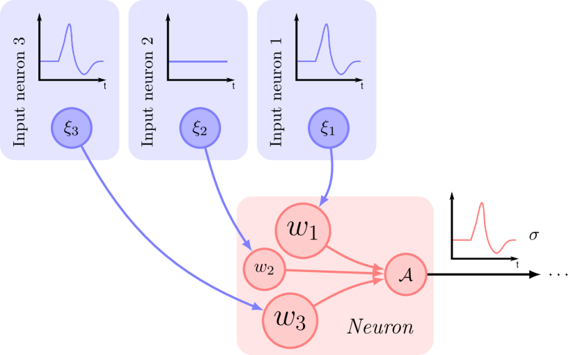
Figure 1: Snapshot in time of a simple neural network. In this small network ($N=3$), the neuron of interest (red) has three input neurons (blue), two of which are just sending a short signal, an action potential, while the second input neuron is silent. This behaviour is captured by input vector ${\bm{\xi}}=\left\{1,-1,1\right\}$ for the network shown. Each of the connections between the neuron of interest and an input neuron has a weight $w_{n}$. The neuron, which is fully characterised by its weights ${\bm{w}}=(w_{1},\dots,w_{N})\in\mathbb{R}^{N}$, will also send an action potential, depending on its activation $\mathcal{A}\sim{\bm{w}}\cdot{\bm{\xi}}$. The response of the neuron is denoted by $\sigma$. In this example, $\sigma=1$.

We consider a single neuron, modeled by a single-layer neural network shown schematically in Fig. 1. In neural networks, individual neurons communicate via action potentials, i.e. short electric pulses that are the basic token of communication in biological neural networks Kandel et al. (2000). The neuron’s task is to decide whether to fire an action potential or not given an input it gets from the $N$ neurons that it is connected to. Since we are not interested in the precise temporal dynamics of the action potentials, we model the input of the neuron, i.e. the signals that the neuron receives at a particular point in time, as vectors ${\bm{\xi}}=(\xi_{1},\dots,\xi_{N})$ where $\xi_{n}=1$ if the $n$th connected neuron is firing an action potential in that input. For symmetry reasons, we set $\xi_{n}=-1$ if the $n$th neuron is silent. The inputs are distributed according to

$$p({\bm{\xi}})=\prod_{n=1}^{N}\frac{1}{2}\left[\delta(\xi_{n}-1)+\delta(\xi_{n}+1)\right].$$ (1)

The neuron itself is fully characterised by the $N$ weights ${\bm{w}}\in\mathbb{R}^{N}$ of its $N$ afferent connections. The weights obey noisy dynamics, to be specified in Sec. III. Presented with a given input ${\bm{\xi}}$, the neuron computes an input-dependent activation

$$\mathcal{A}\equiv\frac{1}{\sqrt{N}}{\bm{w}}\cdot{\bm{\xi}}$$ (2)

where the prefactor ensures normalisation. The activation determines whether the neuron will fire an action potential or not, $\sigma=1$ or $-1$, respectively. If the prediction was noise-free, we would have $\sigma=\operatorname{sgn}(\mathcal{A})$, where $\operatorname{sgn}(x>0)=1$ and $\operatorname{sgn}(x\leq 0)=-1$; instead, the predicted label $\sigma$ is stochastic with

$$p(\sigma|\mathcal{A})\propto\exp(\beta\sigma\mathcal{A})$$ (3)

where $\beta$ is the inverse temperature of the surrounding heat bath. We set $k_{B}=\beta=1$ for the remainder of this article, rendering entropy and energy dimensionless without loss of generality.

The rules we want to learn are Boolean functions of the inputs. More precisely, we will focus on realisable rules which are linearly separable, i.e. we can write

$$\sigma_{\text{T}}=\operatorname{sgn}(\bm{T}\cdot{\bm{\xi}})=\pm 1$$ (4)

where the teacher network $\bm{T}\in\mathbb{R}^{N}$ has the same architecture as the neural network ${\bm{w}}$. The components of the teacher are independent and drawn from a normal distribution with mean 0 and variance 1 and kept fixed. We draw the teacher at random in order to make general statements about the ability of the network to infer teachers of this form. By analogy, the neuron in such a setup is often called the student. We can interpret the true label of an input as an indication of whether the student should fire an action potential in response to that input or not. We emphasise that while the response of a neuron to an input is stochastic, as is the case physiologically, we assume that the teacher does not make mistakes.

The goal of learning is to adjust the weights of the network ${\bm{w}}$ such that the label predicted by the neuron equals the true label for any input ${\bm{\xi}}$, $\sigma=\sigma_{\text{T}}$. The adaptation of weights is thought to be a main mechanism of memory formation in biological networks Kandel et al. (2000). To this end, the neuron needs to infer the teacher $\bm{T}$. However, the neuron only has indirect access to the teacher via a number of samples $({\bm{\xi}}^{\mu},\sigma_{\text{T}}^{\mu})$, where we have now indexed the inputs and their labels with $\mu=1,\dots$, see Fig. 2. The exact form of the dynamics will be specified below in Section III. A classic example for neurons performing this kind of associative learning are the Purkinje cells in the cerebellum Marr (1969); Albus (1971); Ito and Kano (1982); Ito et al. (1982).

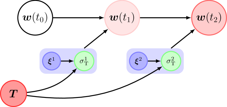
Figure 2: A single neuron learning a rule. The neuron, characterised by its weights ${\bm{w}}\in\mathbb{R}^{N}$, is presented with a succession of inputs ${\bm{\xi}}^{\mu}\in\{-1,1\}^{N}$ and their true labels $\sigma_{\text{T}}^{\mu}=\operatorname{sgn}(\bm{T}\cdot{\bm{\xi}}^{\mu})=\pm 1$ which are determined by a random, static teacher $\bm{T}\in\mathbb{R}^{N}$. The goal of learning is to infer the teacher $\bm{T}$ by using only the information provided by the samples $({\bm{\xi}}^{\mu},\sigma_{\text{T}}^{\mu})$, such that the neuron is eventually able to predict the true label of a previously unseen input.

III Dynamics

Let us now describe the dynamics of the weights learning a rule from a fixed teacher $\bm{T}$. Initially, all the weights are independent of each other and in equilibrium in the potential

$$V({\bm{w}})=\frac{k}{2}{\bm{w}}\cdot{\bm{w}}$$ (5)

which restricts the weights from increasing indefinitely, as is also the case physiologically Dayan and Abbott (2001).

Starting at time $t=0$, the weights $w_{n}$ obey overdamped Langevin equations van Kampen (1992)

$$\dot{w}_{n}(t)=F_{n}\left({\bm{w}}(t),\sigma_{\text{T}}^{\mu(t)},{\bm{\xi}}^{\mu(t)},t\right)+\zeta_{n}(t).$$ (6)

The thermal white noise $\zeta_{n}(t)$ has correlations $\langle\zeta_{n}(t)\zeta_{m}(t^{\prime})\rangle=2D\delta_{nm}\delta(t-t^{\prime})$, where $D$ is the “diffusion” constant. We set the mobility of the weights to unity and impose the fluctuation-dissipation relation $\beta D=1$ for thermodynamic consistency Seifert (2012). For the remainder of this article, we will use angled brackets $\langle\cdot\rangle$ to indicate averages over the thermal noise, unless indicated otherwise.

The total force $\bm{F}=(F_{1},\dots,F_{N})$ on the weights has a conservative contribution from the harmonic potential, $-\nabla V({\bm{w}})=-k{\bm{w}}$, and a non-conservative contribution from the learning force $\bm{f}$, which is a function of a single sample $(\sigma_{\text{T}}^{\mu(t)},{\bm{\xi}}^{\mu(t)})$. The learning force changes the weights in such a way that the neuron becomes more likely to predict the true label for the input as discussed above. In this paper, we focus on online learning, where the learning force changes the weights using just a single sample at a time. The succession of samples is described by the function $\mu(t)=1,2,\dots$. This function may be deterministic or stochastic and we do not make any assumptions about the rate of change of the inputs nor whether the same input may be shown more than once to the neuron. We note that our results also hold for batch learning, where the neuron has simultaneous access to a set of samples at any point in time as discussed in detail in Appendix D.

We will assume that the change to the weights in response to a sample is made in the direction of that input, as is the case for most customary algorithms (see Sec. V and Mace and Coolen (1998); Engel and Van den Broeck (2001); MacKay (2003)). We thus write $\bm{f}=(f_{1},\dots,f_{N})$ with

$$f_{n}\equiv\nu(t)\xi_{n}^{\mu(t)}\sigma_{\text{T}}^{\mu(t)}\mathcal{F}(|{\bm{w}}(t)|,{\bm{w}}(t)\cdot{\bm{\xi}}^{\mu(t)},\bm{T}\cdot{\bm{\xi}}^{\mu(t)}),$$ (7)

where we have introduced a possibly time-dependent learning rate $\nu(t)$ and we denote the Euclidean norm of a vector by $|\cdot|$. Here, $\mathcal{F}$ is an as yet unspecified scalar function of the length of the weight vector, $|{\bm{w}}(t)|$, the student’s field ${\bm{w}}(t)\cdot{\bm{\xi}}^{\mu(t)}$ and the teacher’s field $\bm{T}\cdot{\bm{\xi}}^{\mu(t)}$. The learning force may only depend on the sign of the teacher’s field. Its precise form is specified by learning algorithms; some popular forms are summarised in Tab. 1 and described in more detail in Sec. V. However, we stress that the bounds that we derive in this paper do not depend on the particular form of the learning force and hold for all learning dynamics of the form (6). The full Langevin equation for a weight then reads

$$\dot{w}_{n}(t)=-kw_{n}(t)\\ +\nu(t)\xi^{\mu(t)}_{n}\sigma_{\text{T}}^{\mu(t)}\mathcal{F}(|{\bm{w}}(t)|,{\bm{w}}(t)\cdot{\bm{\xi}}^{\mu(t)},\bm{T}\cdot{\bm{\xi}}^{\mu(t)})+\zeta_{n}(t).$$ (8)

On the ensemble level, the system is fully described by the distribution $p(\bm{T},{\bm{w}},t)$. Its equation of motion is given by a Fokker-Planck equation van Kampen (1992) whose form is simplified by the fact that the noise $\zeta_{n}(t)$ of the different weights is uncorrelated. The dynamics are hence multipartite Hartich et al. (2014); Horowitz (2015) and the Fokker-Planck equation corresponding to the Langevin dynamics (8) separates into one probability current for every weight $w_{n}$,

$$\partial_{t}p(\bm{T},{\bm{w}},t)=-\sum_{n}^{N}\partial_{n}j_{n}(\bm{T},{\bm{w}},t),$$ (9)

where $\partial_{t}\equiv\partial/\partial t$, $\partial_{n}\equiv\partial/\partial w_{n}$ and the probability currents are given by

$$j_{n}(\bm{T},{\bm{w}},t)=\left[-kw_{n}+\nu(t)\xi_{n}^{\mu(t)}\sigma_{\text{T}}^{\mu(t)}\mathcal{F}(|{\bm{w}}|,{\bm{w}}\cdot{\bm{\xi}}^{\mu(t)},\bm{T}\cdot{\bm{\xi}}^{\mu(t)})\right]p(\bm{T},{\bm{w}},t)-D\partial_{n}p(\bm{T},{\bm{w}},t).$$ (10)

There are hence three sources of stochasticity in the system. On the one hand, the fluctuating weights $w(t)$ and the stochastic process of firing an action potential or not, $\sigma$, for a given activation (2) affect the performance of the network. Furthermore, there is randomness in the choice of samples during learning. Since the neuron learns using just a single randomly drawn input and its label at a time, the system performs stochastic gradient descent in the sense that the direction of the learning force fluctuates from one input to the next and only yields the appropriate direction for the weights on average.

IV A first thermodynamic bound on generalising

The aim of the neuron is to predict the label of a previously unseen input ${\bm{\xi}}$ as well as possible. In the following discussion, we consider the generalisation properties of the neuron, i.e. its performance on an input drawn at random from the distribution (1), so we drop the superscript $\mu$ on inputs and labels. We quantify the accuracy of the predictions using information theory MacKay (2003); Cover and Thomas (2006). The a priori uncertainty about the true label of some input, $\sigma_{\text{T}}$, is quantified by the Shannon entropy of the random variable $\sigma_{\text{T}}$ and defined as

$$S(\sigma_{\text{T}})\equiv-\sum_{\sigma_{\text{T}}=\pm 1}p(\sigma_{\text{T}})\ln p(\sigma_{\text{T}})=\ln 2,$$ (11)

where the equality follows from the fact that for an arbitrary input with probability distribution (1), $p(\sigma_{\text{T}}=\pm 1)=1/2$. We have included the variable $\sigma_{\text{T}}$ as an argument to the Shannon entropy in a slight abuse of notation to emphasise that $S(\sigma_{\text{T}})$ is the entropy of the marginalised distribution of just $\sigma_{\text{T}}$. The definition (11) readily carries over to continuous random variables, where the sum is replaced by an integral over the support of the random variable.

The uncertainty about the true label given the label predicted by the neuron $\sigma$ is given by the conditional Shannon entropy

$$S(\sigma_{\text{T}}|\sigma)\equiv -\sum_{\sigma_{\text{T}},\sigma}p(\sigma_{\text{T}},\sigma)\ln p(\sigma_{\text{T}}|\sigma)$$ (12)

$$\leq S(\sigma_{\text{T}})$$ (13)

where $p(\sigma_{\text{T}}|\sigma)=p(\sigma_{\text{T}},\sigma)/p(\sigma)$ and the inequality indicates that, on average, knowing the label predicted by the neuron reduces uncertainty about its true label.

The natural quantity to measure the information learnt by the neuron is the mutual information

$$I(\sigma_{\text{T}}:\sigma)\equiv S(\sigma_{\text{T}})-S(\sigma_{\text{T}}|\sigma)\geq 0$$ (14)

which measures by how much, on average, the uncertainty about $\sigma_{\text{T}}$ is reduced by knowing $\sigma$. If learning and predicting went perfectly, then by knowing the neuron’s output $\sigma$ one could predict the true label $\sigma_{\text{T}}$ with perfect accuracy, such that $S(\sigma_{\text{T}}|\sigma)=0$ and hence $I(\sigma_{\text{T}}:\sigma)=\ln 2$. On the other hand, when the weights are in equilibrium in their potential $V({\bm{w}})$ before learning, there is no correlation between the weights of the student and those of its teacher, such that $I(\sigma_{\text{T}}:\sigma)=0$.

We can connect the mutual information $I(\sigma_{\text{T}}:\sigma)$ to the well-established generalisation error $\epsilon$ of neural networks Mace and Coolen (1998); Engel and Van den Broeck (2001). It gives the probability that the neuron predicts the wrong label for an arbitrary input ${\bm{\xi}}$, assuming that the prediction of the neuron is noise-free, i.e. $\sigma=\operatorname{sgn}({\bm{w}}\cdot{\bm{\xi}})$, and is defined as

$$\epsilon=\langle\theta(-{\bm{w}}\cdot\bm{T})\rangle$$ (15)

where $\theta$ is the Heaviside step function. If the neuron predicted a label based on its activity reliably via $\sigma=\operatorname{sgn}({\bm{w}}\cdot{\bm{\xi}})$ like the teacher, Eq. (4), the mutual information between the true and predicted label for an arbitrarily drawn input could be expressed as

$$I(\sigma_{\text{T}}:\sigma)=\ln 2-S(\epsilon),$$ (16)

where $S(p)=-p\ln p-(1-p)\ln(1-p)$ is the shorthand for the Shannon entropy of a binary stochastic variable with probability $p$. For a realistic neuron, the activity gives only the probability that the neuron will fire an action potential, see Eq. (3), hence Eq. (16) constitutes an upper bound on its actual performance with noisy predictions. In the following, we will focus on deriving thermodynamic bounds on the amount of information that the neuron can learn from its teacher for the ideal case of noise-free predictions.

Thermodynamics enters the picture by considering the free energy costs of the non-equilibrium dynamics of the weights. They can be quantified by the total entropy production $\Delta S^{\text{tot}}_{n}$ of a single weight in the network which is guaranteed to be non-negative by the second law of stochastic thermodynamics and has two contributions: the heat dissipated by the $n$th weight into the connected heat bath, $\Delta Q_{n}$, and the change in Shannon entropy of the marginalised distribution $p(w_{n})$ Seifert (2012).

For a neural network learning with the dynamics (8), we can show both for $N=1$ and in the thermodynamic limit that

$$I(\sigma_{\text{T}}:\sigma)\leq\Delta S^{\text{tot}}_{n}\equiv\Delta S(w_{n})+\Delta Q_{n}$$ (17)

from the second law for the network (see Appendices A and B for details). This suggests the introduction of an efficiency

$$\eta\equiv\frac{I(\sigma_{\text{T}}:\sigma)}{\Delta S(w_{n})+\Delta Q_{n}}\leq 1.$$ (18)

This inequality is our first main result and holds at all times $t>0$ in Eq. (8) and (9).

We note that while this result is superficially similar to the inequality we have derived previously Goldt and Seifert (2017), here we consider an entirely different scenario. In our previous work, there was no teacher; instead, we considered the learning of a number of fixed inputs with true labels drawn at random, such that the true labels were uncorrelated to the inputs and to each other. Hence the concept of a generalisation error did not apply and “the information” was always related to the labels of the fixed set of inputs. Here, we are learning from a number of samples $(\sigma_{\text{T}}^{\mu},{\bm{\xi}}^{\mu})$ which are examples of the function that the teacher performs, Eq. (4). The network tries to infer this function in order to be able to correctly classify previously unseen inputs. What we show here is that the ability to learn from a teacher and generalise accordingly is bound by the total entropy production per weight.

Algorithm	$\mathcal{F}(|{\bm{w}}|,{\bm{w}}\cdot{\bm{\xi}}^{\mu},\sigma_{\text{T}}^{\mu})$	Ref.
Hebbian	1	Hebb (1949); Vallet (1989)
Perceptron	$\theta(-\sigma_{\text{T}}^{\mu}{\bm{w}}\cdot{\bm{\xi}}^{\mu})$	Rosenblatt (1962); Biehl and Riegler (1994)
AdaTron	${\bm{w}}\cdot{\bm{\xi}}^{\mu}/\sqrt{N}\,\theta(-\sigma_{\text{T}}^{\mu}{\bm{w}}\cdot{\bm{\xi}}^{\mu})$	Anlauf and Biehl (1989)

Table 1: Different learning algorithms for a neuron with weights ${\bm{w}}$ online-learning a sample $(\sigma_{\text{T}}^{\mu},{\bm{\xi}}^{\mu})$ together with the colour code used throughout the paper. Here, $\theta(\cdot)$ is the Heaviside step function. References are given to where the algorithm first appeared in a discussion of (the statistical mechanics of) neural learning, to the best of our knowledge. A detailed discussion of the form of these algorithms is given in Sec. V

V Efficiency of different learning algorithms with $N=1$

Let us look at a toy model of a neuron with a single weight. The weight is initially in equilibrium in the harmonic potential $V(w)=kw^{2}/2$. Without loss of generality, we can set $k=\beta=D=1$, making energy, entropy, time and the weights dimensionless. At time $t=0$, the learning rate is suddenly increased from $0$ to a constant value $\nu_{0}$.

The neuron learns using one of the three learning algorithms, each defined by a particular choice of $\mathcal{F}$ and summarised in Tab. 1. The simplest non-trivial choice is $\mathcal{F}=1$, which is Hebbian learning Hebb (1949); Vallet (1989). For such an algorithm, each incoming sample changes the weight by an amount $\sim\sigma_{\text{T}}^{\mu}\xi^{\mu}$. An obvious improvement on this simple algorithm is to only change the weight if the network would currently predict the wrong label for that input, which is achieved by choosing $\mathcal{F}=\theta(-\sigma_{\text{T}}^{\mu}w\xi^{\mu})$. This is the Perceptron algorithm Rosenblatt (1962). A further refinement of this rule is achieved by choosing $\mathcal{F}=|w\xi^{\mu}|\theta(-\sigma_{\text{T}}^{\mu}w\xi^{\mu})$ such that the change in the weights is proportional to the confidence of the neuron in its decision, measured by $|w\xi^{\mu}|$.

The key insight to solve the dynamics in each case is that in one dimension, $\sigma_{\text{T}}^{\mu}\xi^{\mu}=\operatorname{sgn}(T)$ for all $\xi^{\mu}$, which is readily verified. This has the appealing consequence that it is possible to rewrite the Langevin equations for all three learning rules without any mention of the inputs $\xi^{\mu}$. Instead, learning a rule is equivalent to a quench of the potential of the weight from the simple harmonic form $V(w)=w^{2}/2$ to a new $T$-dependent potential $V^{\text{q}}(T,w)$, the exact form of which depends on the learning algorithm chosen. They read

$$V^{\text{q}}(T,w)=\begin{cases}w^{2}/2-\nu_{0}w\operatorname{sgn}(T)\\ w^{2}/2-\nu_{0}w\operatorname{sgn}(T)\theta(-wT)\\ w^{2}/2(1-\nu_{0}\,\operatorname{sgn}(T)\operatorname{sgn}(w)\theta(-w\,\operatorname{sgn}(T)))\end{cases}$$ (19)

for Hebbian, Perceptron and AdaTron learning, respectively. The weight then relaxes to the new equilibrium distribution, which is given by the Boltzmann distribution. The heat dissipated by the weight during this isothermal relaxation is given by

$$\Delta Q=\langle V^{\text{q}}(T,w)\rangle_{0}-\langle V^{\text{q}}(T,w)\rangle_{\text{eq}}$$ (20)

where $\langle\cdot\rangle_{0}$ and $\langle\cdot\rangle_{\text{eq}}$ indicate averages with respect to the distributions of teacher and weight at $t=0$ and after relaxation, respectively.

Figure 3: Efficiency of a toy model with $N=1$. We plot the efficiency $\eta$, Eq. (18) and in the inset the generalisation error $\epsilon$, Eq. (15), as a function of the fixed learning rate $\nu_{0}$ for a neuron with a single weight, $N=1$, learning using the Hebbian   (solid), Perceptron   (long dashed) and AdaTron   (dashed) algorithms. Parameters: $k=\beta=D=1$ without loss of generality.

We plot the efficiency of learning (17) for $t\to\infty$ in Fig. 3 as a function of the learning rate. While the Hebbian algorithm yields the lowest generalisation error, its efficiency is quickly dominated by the heat dissipated, $\Delta Q\sim\nu_{0}^{2}$, resulting in low efficiency. The perceptron algorithm is the most efficient for large $\nu$ and yields a better generalisation performance than the AdaTron algorithm, too (see the inset of Fig. 3).

We finally note that our inequality (17) is sharp for $N=1$. Optimal efficiency $\eta\to 1$ can for example be reached for Hebbian learning with a time-dependent learning rate $\nu(t)$ where we first linearly increase $\nu(t)$ from $0$ to $\nu_{0}$ over a period of time $\tau$ and then keep it at the final value $\nu_{0}$:

$$\nu(t)\equiv\begin{cases}\nu_{0}t/\tau&t<\tau\\ \nu_{0}&t\geq\tau,\end{cases}$$ (21)

which is similar to an example discussed in Goldt and Seifert (2017). In the limit of slow driving $\tau\to\infty$, the dissipated heat $\Delta Q\to 0$. If additionally the learning rate $\nu\to\infty$, the efficiency $\eta\to 1$.

VI Learning in large networks and a second bound

We just saw in Sec. V that for $N=1$, $\xi^{\mu}\operatorname{sgn}(T\xi^{\mu})=\operatorname{sgn}(T)$ which simplifies the analysis because the inputs $\xi^{\mu}$ do not appear explicitly in the equation of motion of the weight. In higher dimensions, we have instead a learning force on the $n$th weight

$$f_{n}\sim\xi_{n}^{\mu}\operatorname{sgn}(\bm{T}\cdot{\bm{\xi}}^{\mu})=\xi_{n}^{\mu}\operatorname{sgn}\left(T_{n}\xi^{\mu}_{n}+\sum_{m\neq n}T_{m}\xi_{m}^{\mu}\right)$$ (22)

which will fluctuate between the desired value $\operatorname{sgn}(T_{n})$ and $-\operatorname{sgn}(T_{n})$ due to the second term inside the sign function, which is effectively a noise term corrupting the signal from the $n$-th component of the teacher. So instead of relaxing to a new equilibrium as seen for $N=1$, the weights relax to a steady state with a constant, positive rate of thermodynamic entropy production Seifert (2012). Our inequality (17) still applies to this process, but it is not very sharp anymore: $I(\sigma_{\text{T}}:\sigma)\sim 1$ and $\Delta S(w_{n})\sim 1$, but a steady state comes with a non-zero rate of heat dissipation, such that $\Delta Q\sim t$. This issue was not addressed in our previous work Goldt and Seifert (2017). In this section, we derive a sharper bound using concepts from steady state thermodynamics Oono and Paniconi (1998).

We start with the explicit expression for the total entropy production of the weights of the network Seifert (2012),

$$\dot{S}^{\text{tot}}(t)=\sum_{n}\int\operatorname{d}\!\bm{T}\operatorname{d}\!{\bm{w}}\;\frac{p(\bm{T},{\bm{w}},t)}{D}\left(\frac{j_{n}(\bm{T},{\bm{w}},t)}{p(\bm{T},{\bm{w}},t)}\right)^{2}\geq 0.$$ (23)

In our problem, the learning rate $\nu(t)$ acts as a control parameter. For every value of $\nu(t)$, there is a well-defined steady state $p^{\text{s}}(\bm{T},{\bm{w}};\nu(t))$ where $\partial_{t}p^{\text{s}}(\bm{T},{\bm{w}};\nu(t))=0$ as in equilibrium, but where at least some of currents $j_{n}^{\text{s}}(\bm{T},{\bm{w}};\nu(t))\neq 0$, leading, inter alia, to a constant rate of total entropy production $\dot{S}^{\text{tot}}\geq 0$ in the steady state. For the remainder of this section, we will use the shorthands

$$p= p(\bm{T},{\bm{w}},t), p^{\text{s}}= p^{\text{s}}\left(\bm{T},{\bm{w}};\nu(t)\right),$$ (24)

$$j_{n}= j_{n}(\bm{T},{\bm{w}},t), j_{n}^{\text{s}}= j_{n}^{\text{s}}\left(\bm{T},{\bm{w}};\nu(t)\right),$$ (25)

to keep our notation slim. We can rewrite the total entropy production (23),

$$\dot{S}^{\text{tot}}(t)= \sum_{n}\int\operatorname{d}\!\bm{T}\operatorname{d}\!{\bm{w}}\;\frac{p}{D}\left(\frac{j_{n}}{p}-\frac{j_{n}^{\text{s}}}{p^{\text{s}}}+\frac{j_{n}^{\text{s}}}{p^{\text{s}}}\right)^{2}$$ (26)

$$= \sum_{n}\int\operatorname{d}\!\bm{T}\operatorname{d}\!{\bm{w}}\;\frac{p}{D}\left(\frac{j_{n}}{p}-\frac{j_{n}^{\text{s}}}{p^{\text{s}}}\right)^{2}+\sum_{n}\int\operatorname{d}\!\bm{T}\operatorname{d}\!{\bm{w}}\;\frac{p}{D}\left(\frac{j_{n}^{\text{s}}}{p^{\text{s}}}\right)^{2}+2\sum_{n}\int\operatorname{d}\!\bm{T}\operatorname{d}\!{\bm{w}}\;\frac{p}{D}\frac{j_{n}^{\text{s}}}{p^{\text{s}}}\left(\frac{j_{n}}{p}-\frac{j_{n}^{\text{s}}}{p^{\text{s}}}\right).$$ (27)

The cross-term is identically zero, which can be seen by first rewriting the integrand and then integrating by parts,

$$\sum_{n}\int\operatorname{d}\!\bm{T}\operatorname{d}\!{\bm{w}}\;\frac{p}{D}\frac{j_{n}^{\text{s}}}{p^{\text{s}}}\left(\frac{j_{n}}{p}-\frac{j_{n}^{\text{s}}}{p^{\text{s}}}\right)$$ (28)

$$= \sum_{n}\int\operatorname{d}\!\bm{T}\operatorname{d}\!{\bm{w}}\;\frac{p}{D}\frac{j_{n}^{\text{s}}}{p^{\text{s}}}D(-\partial_{n}\ln\frac{p}{p^{\text{s}}})$$ (29)

$$= \sum_{n}\int\operatorname{d}\!\bm{T}\operatorname{d}\!{\bm{w}}\;\partial_{n}j_{n}^{\text{s}}\frac{p}{p^{\text{s}}}=0,$$ (30)

where we have used the fact that our system is infinite to integrate and the Fokker-Planck equation in the last step. We can hence write Seifert (2012); Van den Broeck and Esposito (2010)

$$\dot{S}^{\text{tot}}(t)=\dot{S}^{\text{na}}(t)+\dot{S}^{\text{a}}(t)$$ (31)

where we have introduced the non-adiabatic entropy production

$$\dot{S}^{\text{na}}(t)\equiv\sum_{n}\int\operatorname{d}\!\bm{T}\operatorname{d}\!{\bm{w}}\;\frac{p}{D}\left(\frac{j_{n}}{p}-\frac{j_{n}^{\text{s}}}{p^{\text{s}}}\right)^{2}\geq 0$$ (32)

and the adiabatic entropy production

$$\dot{S}^{\text{a}}(t)\equiv\sum_{n}\int\operatorname{d}\!\bm{T}\operatorname{d}\!{\bm{w}}\;\frac{p}{D}\left(\frac{j_{n}^{\text{s}}}{p^{\text{s}}}\right)^{2}\geq 0$$ (33)

Both entropy production rates are evidently positive. They each correspond to a possible mechanism that leads to the breaking of time symmetry and hence to dissipation: the application of non-equilibrium constraints ($\dot{S}^{\text{a}}$) and the presence of driving ($\dot{S}^{\text{na}}$).

The non-adiabatic entropy production of the system can be written as Van den Broeck and Esposito (2010)

$$\dot{S}^{\text{na}}(t)=-\int\operatorname{d}\!\bm{T}\operatorname{d}\!{\bm{w}}\;\dot{p}(\bm{T},{\bm{w}},t)\ln\frac{p(\bm{T},{\bm{w}},t)}{p^{\text{s}}(\bm{T},{\bm{w}},\nu(t))}.$$ (34)

It becomes identically zero once the steady state is reached, as is easily seen from its definition. By splitting the logarithm, we find the second law of steady state thermodynamics Oono and Paniconi (1998); Hatano and Sasa (2001); Van den Broeck and Esposito (2010)

$$\dot{S}^{\text{na}}(t)=\dot{S}(\bm{T},{\bm{w}},t)+\dot{Q}^{\text{ex}}(t)\geq 0$$ (35)

where $\dot{S}(\bm{T},{\bm{w}},t)$ is the rate of change of the Shannon entropy of the distribution $p(\bm{T},{\bm{w}},t)$ and we have identified the excess heat Oono and Paniconi (1998); Van den Broeck and Esposito (2010); Hatano and Sasa (2001)

$$\dot{Q}^{\text{ex}}(t)\equiv\int\operatorname{d}\!\bm{T}\operatorname{d}\!{\bm{w}}\;\dot{p}(\bm{T},{\bm{w}},t)\;\ln p^{\text{s}}(\bm{T},{\bm{w}},\nu(t))$$ (36)

which has no definite sign.

Starting from the second law of steady-state thermodynamics (35), we can derive our second, sharper bound on the accuracy of learning:

$$I(\sigma_{\text{T}}:\sigma)\leq\Delta S(w_{n})+\Delta Q^{\text{ex}}_{n}$$ (37)

which leads to the efficiency

$$\tilde{\eta}\equiv\frac{I(\sigma_{\text{T}}:\sigma)}{\Delta S(w_{n})+\Delta Q^{\text{ex}}_{n}}\leq 1.$$ (38)

This the second main result of our paper. It also holds at all times and applies to any learning algorithm that depends on the weights, ${\bm{w}}$, and samples $(\sigma_{\text{T}}^{\mu(t)},{\bm{\xi}}^{\mu(t)})$. We give the details of its derivation in Appendix C and show that our result applies to batch learning in Appendix D.

VII Online learning in large networks

The number of afferent connections to a single neuron in a realistic network may be on the order of thousands Kandel et al. (2000), so it is sensible to analyse learning in the limit $N\to\infty$. We will focus on online learning Heskes and Kappen (1991); Biehl and Riegler (1994) using the algorithms introduced in Sec. V and summarised in Table 1. We will assume that the samples, indexed by $\mu(t)$, change much faster than the weights relax. This assumption is central to virtually all of the existing literature on the analysis of online learning algorithms.

VII.1 Scaling of the learning rate

We have noted that for $N>2$, the learning force on the $n$th weight will fluctuate between two values proportional to $\pm\operatorname{sgn}(T_{n})$, leading to a steady state with constant $\epsilon$ and constant rate of heat dissipation. Let us try to make this statement more quantitative by looking at the learning force averaged over the inputs ${\bm{\xi}}$ in the limit $N\to\infty$. Setting $\mathcal{F}=1$ for the moment for simplicity of notation, we have

$$f_{n}=\nu(t)\sigma_{\text{T}}^{\mu}\xi^{\mu}_{n}=\nu(t)\xi^{\mu}_{n}\operatorname{sgn}(T_{n}\xi^{\mu}_{n}+\psi)$$ (39)

where we have written $\mu=\mu(t)$ to simplify our notation and we have introduced the noise term inside the $\operatorname{sgn}(\cdot)$ function,

$$\psi\equiv\sum_{m\neq n}T_{m}\xi_{m}^{\mu}.$$ (40)

$\psi$ is uncorrelated with $T_{n}\xi^{\mu}_{n}$ and normally distributed with zero mean and variance $N-1\approx N$ due to the central limit theorem since the teacher and the inputs are uncorrelated. We are interested in the probability $p_{\parallel}$ that

$$\operatorname{sgn}(T_{n}\xi_{n}^{\mu}+\psi)=\operatorname{sgn}(T_{n}\xi_{n}^{\mu}),$$ (41)

i.e. the probability that the learning force points in the right direction despite the noise term $\psi$. This probability is found by integrating the binormal distribution $p(T_{n},\psi)=p(T_{n})p(\psi)$ over the region where (41) holds for $\xi_{n}^{\mu}=1$ and $\xi_{n}^{\mu}=-1$, respectively. We find that

$$\langle f_{n}\rangle_{{\bm{\xi}}}=\nu(t)(2p_{\parallel}-1)\operatorname{sgn}(T_{n})\sim\nu(t)\frac{\operatorname{sgn}(T_{n})}{\sqrt{N}}$$ (42)

where we have expanded $p_{\parallel}$ for large $N$ Olver et al. (2010). Hence the larger the network, the smaller the information that $\sigma_{\text{T}}=\operatorname{sgn}(\bm{T}\cdot{\bm{\xi}})$ carries about a single component of the teacher network. This analysis suggests we choose a learning rate $\nu(t)\equiv\tilde{\nu}_{0}\sqrt{N}$ with the normalised learning rate $\tilde{\nu}(t)\sim 1$. This choice corresponds to the conventional scaling of time with the inverse of the network size in the machine learning literature Mace and Coolen (1998); Engel and Van den Broeck (2001), which amounts to nothing more but an increase in samples shown to the network to compensate for the dilution of the signal.

VII.2 Dynamics

First of all, we would like to compute the time-dependent generalisation error $\epsilon(t)$ for online learning with the three algorithms from Tab. 1 in a large network with dynamics given by (8). We keep the inverse temperature and the diffusion constant at $\beta=D=1$ and again consider the case where the learning rate is quenched to a constant value $\tilde{\nu}=\tilde{\nu}_{0}$ at $t=0$, leaving us with two free parameters: $\tilde{\nu}_{0}$ and the stiffness of the harmonic potential $k$, see Eq. (5).

We thus introduce two new parameters, which go back to the original proof of convergence of the perceptron algorithm Minsky and Papert (1969) and play an important role in the statistical mechanics of learning Engel and Van den Broeck (2001),

$$\mathcal{Q}\equiv\frac{{\bm{w}}\cdot{\bm{w}}}{N}\quad\text{and}\quad\mathcal{R}\equiv\frac{\bm{T}\cdot{\bm{w}}}{N}.$$ (43)

These quantities have the appealing property of being self-averaging in the thermodynamic limit, where they become the second moment of $w_{n}$ and the covariance of $(T_{n},w_{n})$, respectively. Using geometrical Engel and Van den Broeck (2001) or analytical Mace and Coolen (1998) arguments, it can be shown that the generalisation error (15) becomes

$$\epsilon=\frac{1}{\pi}\arccos\left(\frac{{\bm{w}}\cdot\bm{T}}{|{\bm{w}}||\bm{T}|}\right)=\frac{1}{\pi}\arccos\left(\frac{\mathcal{R}}{\sqrt{\mathcal{Q}}}\right).$$ (44)

Hence it is sufficient to find and solve the equations of motion for $\mathcal{Q}$ and $\mathcal{R}$ to solve the dynamics of the generalisation error.

We can indeed derive such equations directly from the Langevin equation for the weights ${\bm{w}}$ (8) (see Appendix E). They read

$$\begin{split}\dot{\mathcal{Q}}=&2(1-k\mathcal{Q})+2\tilde{\nu}_{0}\langle\operatorname{sgn}(x)y\mathcal{F}(x,y)\rangle_{{\bm{\xi}}}\\ &\qquad+\tilde{\nu}_{0}^{2}\langle\mathcal{F}^{2}(x,y)\rangle_{{\bm{\xi}}},\end{split}$$ (45a)

$$\dot{\mathcal{R}}= -k\mathcal{R}+\tilde{\nu}_{0}\langle\operatorname{sgn}(x)x\mathcal{F}(x,y)\rangle_{{\bm{\xi}}},$$ (45b)

where we have introduced the auxiliary random variables

$$x\equiv\bm{T}\cdot{\bm{\xi}}/\sqrt{N}\qquad\text{and}\qquad y\equiv{\bm{w}}\cdot{\bm{\xi}}/\sqrt{N}.$$ (46)

Since we are assuming that the inputs change on a timescale much faster than the relaxation time of the weights, we need to average Eqs. (45) over the inputs ${\bm{\xi}}$. This average is simplified by noting that the inputs only enter the equations via $x$ and $y$. Thus the average over the inputs can be replaced with an average over $x$ and $y$, which are binormally distributed by the central limit theorem, with moments

$$\begin{gathered}\langle x\rangle_{\bm{\xi}}=\langle y\rangle_{\bm{\xi}}=0,\\ \langle x^{2}\rangle_{\bm{\xi}}=1,\quad\langle y^{2}\rangle_{\bm{\xi}}=\mathcal{Q},\quad\langle xy\rangle_{\bm{\xi}}=\mathcal{R}.\end{gathered}$$ (47)

The averages $\langle\cdot\rangle_{\bm{\xi}}$ can be performed analytically for all three learning algorithms and their particular choice of $\mathcal{F}$, see Tab. 1. We give the results in Appendix E. This procedure eventually yields a set of closed equations for $\mathcal{R}$ and $\mathcal{Q}$ for each learning algorithm, which can be solved numerically.

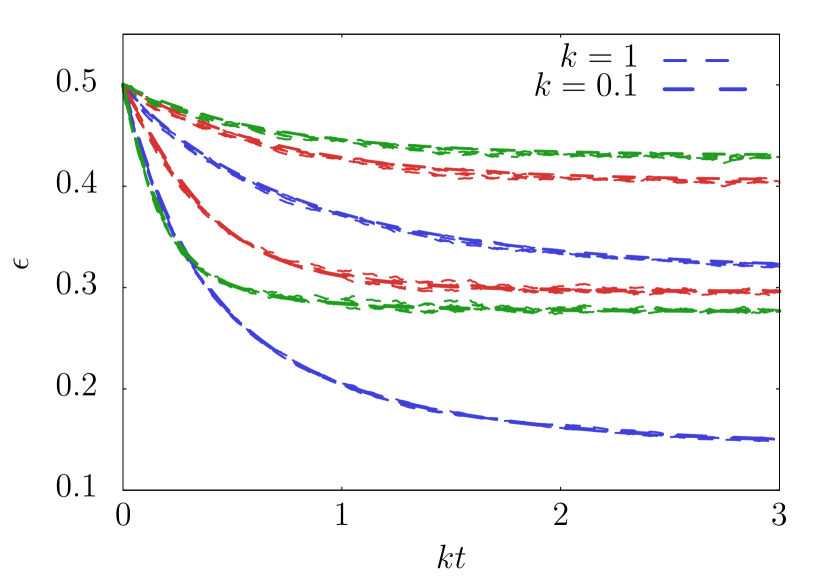
Figure 4: Dynamics of online learning in large networks. We compare the generalisation error $\epsilon$ of online learning in the thermodynamic limit with fixed normalised learning rate $\tilde{\nu}_{0}~{}=~{}1$ computed by solving the equations of motion for $\mathcal{Q}$ and $\mathcal{R}$, Eq. (45) (solid) with the results of numerical simulations of the noisy dynamics of a network with $N~{}=~{}10000$ (dashed) performing online learning using the Hebbian  , Perceptron   and AdaTron   algorithms, plotting five trajectories for each algorithm. Parameters: $\beta=D=1$.

Fig. 4 shows the generalisation error obtained from numerical simulations of the Langevin equation (8) for a network with $N=10000$, $\tilde{\nu}_{0}=\beta=D=1$ and compares it to the result obtained by our analytical calculation that we just discussed. First, we note that $\epsilon$ is a self-averaging quantity, i.e. each simulation run generates the same $\epsilon$ over time within small fluctuations which are scale inversely with $N$. Furthermore, the dynamics of $\epsilon$ are well described by our analytical result. While the Hebbian learning takes the longest time to converge, it is perhaps surprisingly the most robust algorithm in the presence of noise, consistently yielding the lowest generalisation errors. Indeed, for online learning with $k=0$ and no noise, it is well established that $\epsilon$ decays slower for the Perceptron than the Hebbian algorithm; on the other hand, Hebbian learning fails miserably with non-uniform input distributions Engel and Van den Broeck (2001). The performance of the Perceptron is significantly improved by a choice of time-dependent learning rates in a process called annealing. This is beyond the scope of this paper, but see Barkai et al. (1995) for a detailed discussion of the impact of time-dependent learning rates on the convergence of learning algorithms.

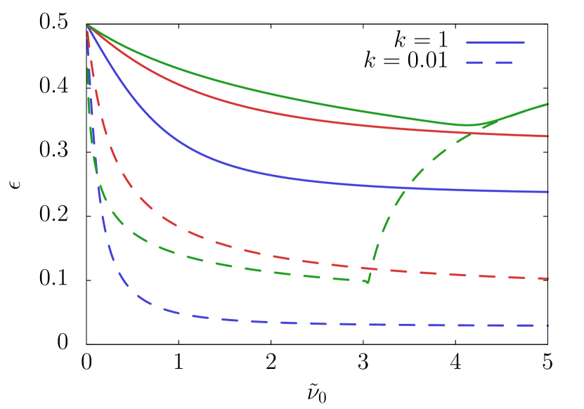
Figure 5: Final generalisation error in large networks. We plot the final, steady-state generalisation error $\epsilon$ of online learning in the thermodynamic limit using Hebbian  , Perceptron   and AdaTron   algorithms. The behaviour of the algorithms and AdaTron learning in particular is discussed in detail in Sec. VII.2. Parameters: $\beta=D=1$.

A remarkable property of AdaTron learning is demonstrated in Fig. 5, where we plot the final, steady-state generalisation error $\epsilon$ against the normalised learning rate $\tilde{\nu}_{0}$. While Hebbian and Perceptron learning (green and blue, resp.) show the expected decrease of $\epsilon$ with $\tilde{\nu}_{0}$, there is a sharp increase of $\epsilon$ for AdaTron learning at $\tilde{\nu}_{c}=3$ (green). Indeed, for large learning rates, the AdaTron algorithm will fail completely. This sensitivity of the algorithm to the value of the learning rate is well-known in the noise-free case without potential $V({\bm{w}})$ Engel and Van den Broeck (2001) and persists in our model with noise, most markedly for low potential stiffness $k$. A detailed analysis of the first-order system $(\mathcal{Q},\mathcal{R})$ reveals that the fixed point with $\epsilon$ close to $1$ becomes unstable as the learning rate crosses the point $\tilde{\nu}_{c}=3$ and a second, stable fixed point emerges with $\epsilon\to 1/2$ (see Appendix F).

VII.3 Efficiency of learning

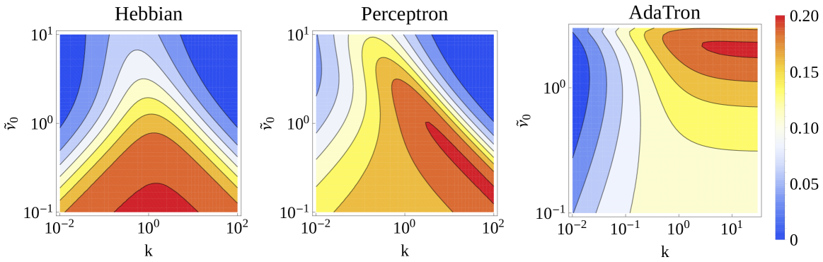
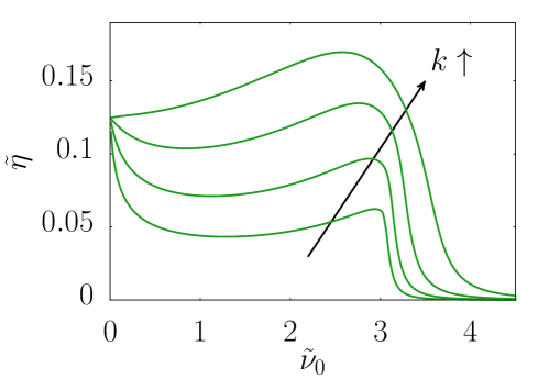
Figure 6: Efficiency of learning in large networks. The efficiency $\tilde{\eta}$, Eq. (38), for neural networks performing online learning with fixed normalised learning rate $\tilde{\nu}_{0}$ using the Hebbian, Perceptron and AdaTron algorithms for online learning in the thermodynamic limit is shown from left to right as a function of the potential stiffness $k$ and $\tilde{\nu}_{0}$. On the far right, we plot the same efficiency $\tilde{\eta}$ of AdaTron learning   versus the normalised learning rate $\tilde{\nu}_{0}$ for increasing values of $k$ from $0.01$ (bottom) to $1$ (top). Parameters: $\beta=D=1$.

We can also derive an ordinary differential equation for the ensemble average of the excess heat (36) in terms of $\mathcal{Q}$ and $\mathcal{R}$, with the details to be found in Appendix G. Since the components of the teacher and the weights are normally distributed, the change in Shannon entropy of the marginalised distribution of a weight $\Delta S(w_{n})$ can be expressed in terms of just $\mathcal{Q}$, giving us all the information necessary to compute the efficiency of learning $\tilde{\eta}$ (38). We plot the efficiency $\tilde{\eta}$ in the thermodynamic limit in Fig. 6 against the normalised learning rate $\tilde{\nu}_{0}$ and the potential stiffness $k$, which are the only remaining free parameters in this model.

The efficiency of Hebbian learning is roughly symmetric with respect to $k$ around $k=1$, while Perceptron and AdaTron learning display highly asymmetric patterns. However, we find that despite the different patterns, the maximum efficiency for all three algorithms is $\eta\simeq 0.2$. We can dig a little deeper by first noting that since $p(T_{n},w_{n})$ is normally distributed for the learning algorithms we have considered, both the mutual information $I(T_{n}:w_{n})$ and the mutual information between the true and the predicted label for an arbitrary input $I(\sigma_{\text{T}}:\sigma)$ can be written as functions of only the correlation between $T_{n}$ and $w_{n}$, $\rho\equiv\mathcal{R}/\sqrt{\mathcal{Q}}$. Expanding around $\rho=0$ yields

$$\frac{I(\sigma_{\text{T}}:\sigma)}{I(T_{n}:w_{n})}=\frac{\ln 2-S(\arccos(\rho)/\pi)}{-1/2\ln(1-\rho^{2})}=\frac{4}{\pi^{2}}+\mathcal{O}(\rho^{2})\simeq 0.4$$ (48)

which turns out to be a good approximation for $\rho\lesssim 0.9$. So at maximum efficiency,

$$\frac{I(w_{n}:T_{n})}{\Delta S(w_{n})+\Delta Q^{\text{ex}}_{n}}\simeq\frac{1}{2}$$ (49)

for all three algorithms.

The last plot in Fig. 6 shows that the bifurcation we discussed for the AdaTron learning in Sec. VII.2 leads to a decaying efficiency $\tilde{\eta}\to 0$ since $I(\sigma_{\text{T}}:\sigma)\to 0$. This effect is smoothed out with increasing potential stiffness.

Let us finally note that, in this model, the rate of heat dissipation of a single weight diverges in the thermodynamic limit, $\dot{Q}_{n}\to\infty$ as $N\to\infty$. This is readily understood from a physical point of view since the weights experience a large force, $f\sim\sqrt{N}$, which fluctuates very quickly. This observation reinforces the importance of our second bound involving the excess heat (36), which does not diverge even in the limit $N\to\infty$.

VIII Concluding perspectives

We have analysed the learning of linearly separable rules by neural networks as a model for the thermodynamics of generalisation. Using stochastic thermodynamics and information theory, we have shown that the accuracy with which the neuron is able to apply the rule to previously unseen inputs is constrained by the dissipation of free energy of a single weight during the learning process. Our results hold for all learning algorithms that have access to all the weights, ${\bm{w}}$, and either a set of or a succession of samples $(\sigma_{\text{T}}^{\mu(t)},{\bm{\xi}}^{\mu(t)})$ in batch or online learning, respectively. We have furthermore given a detailed analysis of both the dynamics and the thermodynamics of online learning in large neural networks with noisy dynamics and weights constrained by an external potential.

It is worthwhile to revisit the results of our earlier work Goldt and Seifert (2017) in the light of these results. In this previous paper, we studied a different learning problem, namely the learning of $P$ mappings ${\bm{\xi}}^{\mu}\to\sigma_{\text{T}}^{\mu}$ from fixed inputs ${\bm{\xi}}^{\mu}$, $\mu=1,\ldots,P$ to their true labels $\sigma_{\text{T}}^{\mu}$. The true labels were drawn at random for each input, and hence uncorrelated to the inputs and to each other. Hence there is no generalisation error for this problem – if the true label of every input is determined by pure chance, the mappings $\left\{{\bm{\xi}}^{\mu}\to\sigma_{\text{T}}^{\mu}\right\}_{\mu=1}^{P}$ carry no information about the label of a previously unseen input. Instead, the challenge is to find a set of weights that reproduce the mappings faithfully.

The two problems are however related in the following way. It is possible to at least construct a teacher $\bm{T}$ that reproduces all the mappings ${\bm{\xi}}^{\mu}\to\sigma_{\text{T}}^{\mu}$ using $\sigma_{\text{T}}^{\mu}=\operatorname{sgn}(\bm{T}\cdot{\bm{\xi}}^{\mu})$ if and only if the number of mappings $P$ is less than the capacity of the network. This capacity is usually defined in the thermodynamic limit, where the number of weights $N\to\infty$, and we are interested in the relative number of inputs $\alpha_{c}\equiv P_{c}/N\sim 1$ for which there exists a teacher $\bm{T}$ that reproduces all the true labels via $\sigma_{\text{T}}=\operatorname{sgn}(\bm{T}\cdot{\bm{\xi}})$ with probability 1 MacKay (2003). Its numerical value can be derived analytically from replica calculations Gardner (1987), but it was first understood using geometrical arguments Polya (1954); Cover (1965) (see also MacKay (2003) for a pedagogical discussion).

If it is possible to construct a teacher $\bm{T}$, the rule implicitly defined by the mappings is realisable and can, at least in theory, be learned. Even in that case, however, the issue remains for the scenario considered in Goldt and Seifert (2017) that the number of samples from which the neuron learns is limited and might not be sufficient to learn the underlying “rule” effectively. On the other hand, learning the mappings $\left\{{\bm{\xi}}^{\mu}\to\sigma_{\text{T}}^{\mu}\right\}_{\mu}^{P}$ is still a meaningful task even if it is not possible to even construct a network that reproduces them all, if one is willing to accept a certain error in the predictions of the network.

Neurons with a single-layer architecture described here are generally limited to the implementation of linearly separable Boolean functions ${\bm{\xi}}\to\pm 1$. A natural generalisation is to consider networks with several layers, where the output of the neurons in one layer is the input for the neurons in the next layer Engel and Van den Broeck (2001); MacKay (2003). The capabilities of networks with intermediate layers are remarkable: a network of binary neurons ($\sigma=\pm 1$) with just a single intermediate layer can implement any Boolean function of its inputs Denker et al. (1987), while a network with continuous neurons ($\sigma\in\mathbb{R}$, e.g. $\sigma=\tanh(\mathcal{A})$) is capable of approximating any function of its inputs to any required accuracy Cybenko (1989). However, the analysis of these networks is much more involved than that of the single-layer feedforward network discussed here and is left for future work.

Besides the generalisation to networks with intermediate layers of neurons, this work opens up numerous other avenues for further research. It would be intriguing to consider the generalisation of our model to multi-valued teacher functions, e.g. for a network learning to classify digits. The teacher could also be made subject to noise in its outputs $\sigma_{\text{T}}$, or its components, $T_{n}$, or both. Another intriguing learning problem is that of a changing environment, modeled by a drifting teacher Kinouchi and Caticha (1993); Biehl and Schwarze (1993). Designing a learning algorithm that optimises the thermodynamic efficiency looks like a serious challenge. More broadly, studying the thermodynamic costs of learning to generalise might form a suitable basis to consider the thermodynamics of decision-making Colabrese et al. (2017).

We have considered the limitations on computation in neural networks that are a consequence of the second law of thermodynamics and account for the free energy costs of computations. However, there are further limiting factors on the ability to compute. One is the availability of data: for a given inference problem, such as inferring a teacher $\bm{T}$ from a number of samples $(\sigma_{\text{T}},{\bm{\xi}})$, there is a minimum amount of data that is required to make any prediction that is better than simply flipping a coin. A second limiting factor is time: ideally, we would like to have an algorithm whose completion time scales polynomially with the system size, rather than exponentially. It has recently become clear that these two constraints can be understood using statistical mechanics in terms of phase transitions Zdeborová and Krzakala (2016). It will be interesting to see whether the thermodynamic limits that we have derived in this paper fit into this picture, and if so, where they can be found.

Appendices

The following appendices give a detailed proof of our main results, inequalities (17) and (37), in Appendices A to C. Appendix D discusses how our results apply to batch learning. Detailed calculations for the learning dynamics in the thermodynamic limit are given in Appendices E to G.

Appendix A Derivation of inequality (17)

Our first main result, Eq. (17), can be derived from the second law of stochastic thermodynamics Seifert (2012) which states that the rate of total entropy production of the full system is positive

$$\dot{S}^{\text{tot}}(t)\geq 0.$$ (50)

We will drop the explicit time argument in the following discussion but emphasise that since the distribution $p(\bm{T},{\bm{w}},t)$ is time-dependent, so are of course all the quantities derived from it.

We discussed in Sec. III that the total probability current of the system decomposes into a separate current due to the fluctuations in every subsystem $w_{n}$, see Eq. (9). As a consequence, the rate of total entropy production $\dot{S}^{\text{tot}}$ of the network can be split into separate, non-negative contributions due to the fluctuations of every subsystem $w_{n}$, $\dot{S}^{\text{tot}}_{n}$, each of which can further be split into two separate contributions, so that we have

$$\dot{S}^{\text{tot}}=\sum_{n}\dot{S}^{\text{tot}}_{n}=\sum_{n}\dot{S}_{n}({\bm{w}},\bm{T})+\sum_{n}\dot{S}^{\text{m}}_{n}\geq 0.$$ (51)

The first part is the rate of change of the Shannon entropy of the full distribution $p(\bm{T},{\bm{w}},t)$ due to the dynamics of $w_{n}$ and reads

$$\dot{S}_{n}(\bm{T},{\bm{w}})=-\int\operatorname{d}\!\bm{T}\operatorname{d}\!{\bm{w}}\;j_{n}(\bm{T},{\bm{w}})\partial_{n}\ln p(\bm{T},{\bm{w}}).$$ (52)

while the rate of thermodynamic entropy production in the medium by the $n$th weight is given by

$$\dot{S}^{\text{m}}_{n}=\int\operatorname{d}\!\bm{T}\operatorname{d}\!{\bm{w}}\;j_{n}(\bm{T},{\bm{w}})F_{n}(\bm{T},{\bm{w}})$$ (53)

for with the temperature set to unity.

Writing $p(\bm{T},{\bm{w}})=p(w_{n})p(\bm{T},\overline{{\bm{w}}}_{n}|w_{n})$ where $\overline{{\bm{w}}}_{n}\equiv(w_{1},\dots,w_{n-1},w_{n+1},\dots,w_{N})$, we have

$$\dot{S}_{n}(\bm{T},{\bm{w}})=\partial_{t}S(w_{n})-l_{n}(w_{n}:\bm{T},\overline{{\bm{w}}}_{n})$$ (54)

where $\partial_{t}S(w_{n})$ is the change of the Shannon entropy (11) of the marginalised distribution $p(w_{n})=\int\operatorname{d}\!\bm{T}\operatorname{d}\!\overline{{\bm{w}}_{n}}\;p(\bm{T},{\bm{w}})$ due to the dynamics of the $n$th weight. Throughout this paper, we use the dot notation to denote time-dependent rates, as opposed to the time derivative of state functions like the Shannon entropy. The second term in Eq. (54) is an information-theoretic piece which gives the rate at which the dynamics of $w_{n}$ changes its correlations with the other degrees of freedom in the system, namely the other weights $\overline{{\bm{w}}}_{n}$ and the teacher $\bm{T}$, as measured by the mutual information $I(w_{n}:\bm{T},\overline{{\bm{w}}}_{n})$. This quantity has been introduced as the (thermodynamic) learning rate Allahverdyan et al. (2009); Hartich et al. (2014), not to be confused with the learning rate $\nu(t)$ introduced in Eq. (7), or the “information flow” Horowitz and Esposito (2014); Horowitz (2015). Its explicit form is

$$l_{n}(w_{n}:\bm{T},\overline{{\bm{w}}}_{n})=\\ \int\operatorname{d}\!\bm{T}\operatorname{d}\!{\bm{w}}\;j_{n}(\bm{T},{\bm{w}},t)\partial_{n}\ln p(\bm{T},\overline{{\bm{w}}}_{n}|w_{n}).$$ (55)

We finally note that for the isothermal environment that we assume in this paper, the rate of thermodynamic entropy production is the heat dissipated into the environment, $\dot{S}^{\text{m}}_{n}=\dot{Q}_{n}$, where we remind ourselves that we have set the temperature to unity.

Putting it all together, we can formulate the second law for a subsystem,

$$\dot{S}^{\text{tot}}_{n}=\partial_{t}S(w_{n})+\dot{Q}_{n}-l_{n}(w_{n}:\bm{T},\overline{{\bm{w}}}_{n})\geq 0.$$ (56)

which is the starting point of our derivation.

Integrating the $N$ second laws (56) with respect to time from $t^{\prime}=0$ to $t>0$ yields

$$\sum_{n}^{N}\left[\Delta S(w_{n})+\Delta Q_{n}\right]\geq\sum_{n}^{N}\int_{0}^{t}\operatorname{d}\!t^{\prime}\;l_{n}(w_{n}:\bm{T},\overline{{\bm{w}}}_{n})$$ (57)

where we write $\Delta S(w_{n})$ and $\Delta Q_{n}$ to denote the total change in Shannon entropy of the distribution $p(w_{n})$ and the total heat dissipated by the dynamics of the $n$th weight up to time $t$, respectively. We can interpret the right-hand side of (57) by computing the time-derivative of the mutual information $I(\bm{T}:{\bm{w}})$,

$$\partial_{t}I(\bm{T}:{\bm{w}})=\int\operatorname{d}\!\bm{T}\operatorname{d}\!{\bm{w}}\;\left[\partial_{t}p(\bm{T},{\bm{w}},t)\right]\ln\frac{p(\bm{T},{\bm{w}},t)}{p(\bm{T},t)p({\bm{w}},t)}.$$ (58)

Using the Fokker-Planck Eq. (9) and integrating by parts, we find

$$\partial_{t}I(\bm{T}:{\bm{w}})= \sum_{n}^{N}\int\operatorname{d}\!\bm{T}\operatorname{d}\!{\bm{w}}\;j_{n}(\bm{T},{\bm{w}},t)\partial_{n}\ln\frac{p(\bm{T},{\bm{w}},t)}{p(\bm{T},t)p({\bm{w}},t)}$$ (59)

$$= \sum_{n}^{N}\int\operatorname{d}\!\bm{T}\operatorname{d}\!{\bm{w}}\;j_{n}(\bm{T},{\bm{w}},t)\partial_{n}\ln\frac{p(\bm{T},{\bm{w}},t)}{p(w_{n},t)p(\overline{{\bm{w}}}_{n}|w_{n},t)}$$ (60)

$$= \sum_{n}^{N}l_{n}(w_{n}:\bm{T},\overline{{\bm{w}}}_{n})-\sum_{n}^{N}\int\operatorname{d}\!\bm{T}\operatorname{d}\!{\bm{w}}\;j_{n}(\bm{T},{\bm{w}},t)\partial_{n}\ln p(\overline{{\bm{w}}}_{n}|w_{n},t)$$ (61)

$$= \sum_{n}^{N}l_{n}(w_{n}:\bm{T},\overline{{\bm{w}}}_{n})-\left(-\partial_{t}S({\bm{w}})+\sum_{n}^{N}\partial_{t}S(w_{n})\right)$$ (62)

where in the penultimate line, we have recovered the integrand on the right-hand side of (57). Integrating the term in brackets in Eq. (62) with respect to time yields for all times $t>0$

$$\int_{0}^{t}\operatorname{d}\!t^{\prime}\;\left(\sum_{n}^{N}\partial_{t^{\prime}}S(w_{n})-\partial_{t^{\prime}}S({\bm{w}})\right)=\sum_{n}^{N}S(w_{n})-S({\bm{w}})\geq 0$$ (63)

where we have used that at time $t=0$, all the weights are independent of each other and hence $S({\bm{w}})=\sum_{n}S(w_{n})$. The inequality follows from the fact that for any set of random variables, $\sum_{n}S(w_{n})\geq S({\bm{w}})$ Cover and Thomas (2006). Using this inequality, we can deduce from (62) that

$$\sum_{n}^{N}\left[\Delta S(w_{n})+\Delta Q_{n}\right]\geq\sum_{n}^{N}\int_{0}^{t}\operatorname{d}\!t^{\prime}\;l_{n}(w_{n}:\bm{T},\overline{{\bm{w}}}_{n})\geq I(\bm{T}:{\bm{w}}).$$ (64)

Using the chain rule of mutual information Cover and Thomas (2006) and the fact that the components $\bm{T}$ are independent of each other (Sec. II), we have

$$I(\bm{T}:{\bm{w}})= \sum_{n}^{N}I(T_{n}:{\bm{w}}|T_{n-1},\dots,T_{1})$$ (65)

$$\begin{split}=&\sum_{n}^{N}I(T_{n}:{\bm{w}},T_{n-1},\dots,T_{1})-\\ &\qquad\sum_{n}^{N}I(T_{n}:T_{n-1},\dots,T_{1})\end{split}$$ (66)

$$\geq \sum_{n}^{N}I(T_{n}:{\bm{w}})$$ (67)

$$= \sum_{n}^{N}I(T_{n}:w_{n})+I(T_{n}:\overline{{\bm{w}}}_{n}\,|\,w_{n})$$ (68)

$$\geq NI(T_{n}:w_{n})$$ (69)

where the inequalities follow again from the non-negativity of mutual information and the fact that all the weights and all the components of the teacher are statistically identical. Using the latter argument for the total entropy production and inserting our last result into the integrated form of the second law (57), we find that

$$\Delta S(w_{n})+\Delta Q_{n}\geq I(w_{n}:T_{n})$$ (70)

Finally, we need to show that the mutual information between the $n$th component of the weight and teacher vectors are an upper bound on the mutual information between the true and predicted labels of any sample ${\bm{\xi}}$,

$$I(w_{n}:T_{n})\geq I(\sigma_{\text{T}}:\sigma).$$ (71)

Our strategy will be to show that the inequality (71) holds even if the neuron predicts a label deterministically, $\sigma=\operatorname{sgn}({\bm{w}}\cdot{\bm{\xi}})$. The generalisation error is then the lowest for a given noise level in the weights and given by $I(\sigma_{\text{T}}:\sigma)=\ln 2-S(\epsilon)$.

Let us first consider a network with $N=1$. We start by noting that for arbitrary random variables $X$ and $Y$ and an arbitrary function $F(Y)$, we can always write $p(x,y,f(y))=p(x)p(y|x)p\left(f(y)|y\right)$. We thus identify $X\to Y\to F$ as a Markov chain and find

$$I(X:Y)\geq I(X:F)$$ (72)

using the data processing inequality Cover and Thomas (2006). For $N=1$, we can apply this result twice to show that

$$I(w:T)\geq I(w\xi:T\xi)\geq I(\sigma:\sigma_{\text{T}})$$ (73)

as required.

In the thermodynamic limit $N\to\infty$, we use the auxiliary variables $x\equiv{\bm{w}}\cdot{\bm{\xi}}/\sqrt{N}$ and $y\equiv\bm{T}\cdot{\bm{\xi}}/\sqrt{N}$. We then have from (72)

$$I(\sigma_{\text{T}}:\sigma)\leq I(x:y)$$ (74)

since $\sigma_{\text{T}}$ and $\sigma$ are functions of $x$ and $y$, Eq. (4) and Eq. (3), respectively. We can now average $x$ and $y$ over the inputs (1) using $\langle\xi_{n}\rangle_{\xi}=0$ and $\langle\xi_{n}\xi_{m}\rangle_{\xi}=\delta_{nm}$. By the central limit theorem, $x$ and $y$ are then distributed according to a bivariate Gaussian distribution with correlation Cover and Thomas (2006)

$$\rho\equiv\frac{\text{cov}(w_{n},T_{n})}{\text{sd}(w_{n})\,\text{sd}(T_{n})}=\frac{{\bm{w}}\cdot\bm{T}}{|{\bm{w}}||\bm{T}|}$$ (75)

This is a crucial step in our derivation since it allows us to connect the statistics of teacher and weight in one dimension to the statistics of the true and predicted labels, which are functions of the vectors $\bm{T}$ and ${\bm{w}}$. The mutual information of two variables with a bivariate Gaussian distribution is a function of their correlation alone Cover and Thomas (2006),

$$I_{G}(w_{n}:T_{n})=-\frac{1}{2}\left(1-\ln\rho^{2}\right)=I(x:y)$$ (76)

which would also be the mutual information $I(w_{n}:T_{n})$ if $w_{n}$ and $T_{n}$ were jointly distributed normally, which they are not necessarily. However, we can show that $I_{G}(w_{n}:T_{n})$ is a lower bound on $I(w_{n}:T_{n})$ using the maximum entropy principle. This is a prescription for finding the probability distribution that maximises the Shannon entropy given a number of constraint on the distribution, usually in the form of fixed moments. We briefly review this concept in Appendix B. The crucial point here is that a Gaussian distribution is the maximum entropy distribution for a given covariance matrix. We will denote the maximum entropy notations with an asterisk, e.g. $p^{*}$.

The mutual information $I(w_{n}:T_{n})$ can be expressed as the relative entropy or Kullback-Leibler divergence between the joint distribution $p(w_{n},T_{n})$ and the factorised distribution $p(T_{n})p(w_{n})$ Cover and Thomas (2006):

$$I(w_{n}:T_{n})= D\left[p(T_{n},w_{n})||p(T_{n})p(w_{n})\right]$$ (77)

$$\equiv \int\operatorname{d}\!\bm{T}\operatorname{d}\!{\bm{w}}\;p(\bm{T},{\bm{w}})\ln\frac{p(\bm{T},{\bm{w}})}{p(\bm{T})p({\bm{w}})}$$ (78)

where the inequality is true for arbitrary probability distributions. Introducing the shorthand $p(w_{n})\equiv p_{w}$ etc. to simplify notation, we hence are left to show that

$$I(w_{n}:T_{n})-I_{G}(w_{n}:T_{n})$$

$$= \langle\ln\frac{p_{Tw}}{p_{T}p_{w}}\rangle_{p}-\langle\ln\frac{p^{*}_{Tw}}{p^{*}_{T}p^{*}_{w}}\rangle_{p^{*}}$$

$$= \langle\ln p_{Tw}\rangle_{p}-\langle\ln p^{*}_{Tw}\rangle_{p*}$$

$$\quad-\left[\langle\ln p_{T}\rangle_{p}-\langle\ln p^{*}_{T}\rangle_{p^{*}}+\langle\ln p_{w}\rangle_{p}-\langle\ln p^{*}_{w}\rangle_{p^{*}}\right]$$

$$= \langle\ln p_{Tw}\rangle_{p}-\langle\ln p^{*}_{Tw}\rangle_{p}$$

$$\quad-\left[\langle\ln p_{T}\rangle_{p}-\langle\ln p^{*}_{T}\rangle_{p}+\langle\ln p_{w}\rangle_{p}-\langle\ln p^{*}_{w}\rangle_{p}\right]$$

$$= D\left[p_{Tw}||p^{*}_{Tw}\right]-D\left[p_{T}||p^{*}_{T}\right]-D\left[p_{w}||p^{*}_{w}\right]$$

$$= D\left[p_{T|w}||p^{*}_{T|w}\right]\geq 0$$

where we used that $\langle\ln p^{*}_{Tw}\rangle_{p^{*}}=\langle\ln p^{*}_{Tw}\rangle_{p}$ for the third equality, see Sec. B, while for the last equality we applied the chain rule for the Kullback-Leibler distance Cover and Thomas (2006) and remembered that $p(T_{n})$ is a Gaussian distribution and hence the maximum entropy distribution for a given variance. This completes our derivation of the bound (17).

Appendix B Surprise and maximum entropy distributions

We briefly review the concept of a maximum entropy distributions, which have a long history in physics Jaynes (1957). We will focus on the case of a single variable to illustrate the concepts, but we note that the multi-dimensional case can be treated using the same methods.

We are looking for a probability distribution $p$ of a continuous variable $X$ with support $\mathcal{S}$ which is subject to $M$ constraints, namely

$$\int_{\mathcal{S}}\operatorname{d}\!x\;p(x)r_{i}(x)=\alpha_{i}.$$ (79)

The maximum entropy prescription for finding the distribution $p(x)$ is to find the distribution that maximises the Shannon entropy $S(X)$ (11) under the constraints (79). This is a standard calculation using variational calculus; here we simply quote the result Cover and Thomas (2006),

$$p^{*}(x)\sim\exp\left(\lambda_{0}-1+\sum_{i}^{M}\lambda_{i}r_{i}(x)\right)$$ (80)

where $\lambda_{i}$ are the Lagrange multipliers chosen such that $p(x)$ obeys the constraints. Proving that (80) is a maximum is a rather involved calculation and is more easily proven using information-theoretic methods Cover and Thomas (2006).

The key point for our purposes is that for a distribution $p(x)$, which is unknown except for a number of its moments, averaging the surprise $\ln p^{*}(x)$ of the maximum entropy distribution for the known moments over $p^{*}$ is equal to the average taken with respect to the true distribution $p$,

$$\langle\ln p^{*}(x)\rangle_{p^{*}}=\langle\ln p^{*}(x)\rangle_{p}.$$ (81)

This result is a direct consequence of the form of the maximum entropy distribution and the fact that the moments that enter $p^{*}$ are by construction equal to the corresponding moments of $p$.

Appendix C Derivation of inequality (37)

The non-adiabatic entropy production of the $n$th single weight is defined as

$$\dot{S}^{\text{na}}_{n}(t)\equiv\int\operatorname{d}\!\bm{T}\operatorname{d}\!{\bm{w}}\;p\left(\frac{j_{n}}{p}-\frac{j_{n}^{\text{s}}}{p^{\text{s}}}\right)^{2}\geq 0,$$ (82)

see Sec. VI for a detailed discussion. Summing $\dot{S}^{\text{na}}_{n}(t)$ over all subsystems, we find

$$\sum_{n}\dot{S}^{\text{na}}_{n}(t)=\sum_{n}\dot{S}_{n}(\bm{T},{\bm{w}})+\sum_{n}\dot{Q}^{\text{ex}}_{n}\geq 0$$ (83)

where the rate of excess heat production $\dot{Q}^{\text{ex}}_{n}$ was defined in Eq. (36). After writing $\dot{S}_{n}(\bm{T},{\bm{w}})=\partial_{t}S(w_{n})-l_{n}(w_{n}:\bm{T},\overline{{\bm{w}}}_{n})$ and integrating over time, see the discussion in Appendix A, we find that

$$\sum_{n}^{N}\left[\Delta S(w_{n})+\Delta Q^{\text{ex}}_{n}\right]\geq\sum_{n}^{N}\int_{0}^{t}\operatorname{d}\!t^{\prime}\;l_{n}(w_{n}:\bm{T},\overline{{\bm{w}}}_{n}).$$ (84)

and we can now proceed along the lines of Appendix A.

Appendix D Batch learning

Our discussion has focused on online learning, where, at any one point in time, the network experiences a learning force $\bm{f}$ due to a single input and its label, Eq. (7). Another approach is to average the learning force over a set $D=\left\{(\sigma_{\text{T}}^{\mu},{\bm{\xi}}^{\mu})\right\}_{\mu=1}^{P}$ of $P$ inputs and their labels,

$$f_{n}\equiv\nu(t)\langle\xi_{n}^{\mu}\sigma_{\text{T}}^{\mu}\mathcal{F}(|{\bm{w}}(t)|,{\bm{w}}(t)\cdot{\bm{\xi}}^{\mu},\bm{T}\cdot{\bm{\xi}}^{\mu})\rangle_{D}.$$ (85)

This strategy is called batch learning and $P$ is usually chosen to be on the order of $N$. In the thermodynamic limit, as $N\to\infty$ one thus lets $P\to\infty$ while keeping the ratio $\alpha\equiv P/N$ on the order of one.

Batch learning clearly comes with high requirements in terms of memory. It is generally more efficient than online learning, although the latter can achieve generalisation errors which at least asymptotically match the results from batch learning Engel and Van den Broeck (2001).

Our two main results, inequalities (17) and (37) apply to batch learning as well. This is because in our derivation, we only used the fact that the teacher enters the force on the weights, albeit indirectly. We did not have to specify the exact form of the learning force that introduces the correlations between the weight and the teacher. Hence it does not make a difference in the derivation of the inequalities whether the learning force is computed for just a single sample or averaged over a set of samples.

Appendix E Solving the learning dynamics in the thermodynamic limit

Here we give a detailed derivation of the equations of motion for the order parameters $\mathcal{Q}$ and $\mathcal{R}$ introduced in Sec. VII in the thermodynamic limit $N\to\infty$. These are most easily derived by rewriting the Langevin equations for the weights, Eq. (8), as Itô stochastic differential equations Gardiner (2009)

$$\operatorname{d}\!{\bm{w}}(t)=-k{\bm{w}}(t)\operatorname{d}\!t+\nu(t){\bm{\xi}}^{\mu(t)}\sigma_{\text{T}}^{\mu(t)}\mathcal{F}(|{\bm{w}}(t)|,{\bm{w}}(t)\cdot{\bm{\xi}}^{\mu(t)},\bm{T}\cdot{\bm{\xi}}^{\mu(t)})\operatorname{d}\!t+\operatorname{d}\!\bm{W}(t).$$ (86)

The random Wiener process has components $\operatorname{d}\!W_{n}(t)$ which are normally distributed with mean 0 and variance $2D\operatorname{d}\!t=2\operatorname{d}\!t$ in our choice of units. It is related to the noise term of the Langevin equation via $\operatorname{d}\!W_{n}(t)=\int_{t}^{t+\operatorname{d}\!t}\operatorname{d}\!t^{\prime}\zeta_{n}(t^{\prime})$; see Gardiner (2009) for more details. All other symbols take the same meaning as discussed before Eq. (8). We assume that the inputs that enter the equation are changing on a timescale much faster than the relaxation time of the weights. Hence it is only the statistical properties of the inputs that determine the dynamics of ${\bm{w}}$ in the thermodynamic limit. We can thus average over the inputs, making the detailed dynamics of $\mu(t)$ unimportant. We can derive the equations of motion for the means of $\mathcal{Q}\equiv{\bm{w}}\cdot{\bm{w}}/N$ and $\mathcal{R}\equiv\bm{T}\cdot{\bm{w}}/N$ by expanding to second order in $\operatorname{d}\!{\bm{w}}$ and keeping terms on the order of $\operatorname{d}\!t$:

$$\operatorname{d}\!\mathcal{Q}\equiv \mathcal{Q}({\bm{w}}+\operatorname{d}\!{\bm{w}})-\mathcal{Q}({\bm{w}})$$ (87)

$$= \frac{1}{N}\left(2{\bm{w}}\cdot\operatorname{d}\!{\bm{w}}+\operatorname{d}\!{\bm{w}}\cdot\operatorname{d}\!{\bm{w}}\right)$$

$$= 2(1-k\mathcal{Q})\operatorname{d}\!t+\tilde{\nu}(t)^{2}\langle\mathcal{F}(\sqrt{\mathcal{Q}},\bm{T}\cdot{\bm{\xi}},{\bm{w}}\cdot{\bm{\xi}})^{2}\rangle\operatorname{d}\!t+2\tilde{\nu}(t)\langle\operatorname{sgn}(\bm{T}\cdot{\bm{\xi}})\frac{{\bm{w}}\cdot{\bm{\xi}}}{\sqrt{N}}\mathcal{F}(\sqrt{\mathcal{Q}},\bm{T}\cdot{\bm{\xi}},{\bm{w}}\cdot{\bm{\xi}})\rangle\operatorname{d}\!t$$

where, contrary to ordinary calculus, the term $\operatorname{d}\!{\bm{w}}\cdot\operatorname{d}\!{\bm{w}}$ has contributed two terms, one from the Wiener process and one because ${\bm{\xi}}\cdot{\bm{\xi}}\approx N\approx 1/\operatorname{d}\!t$. We have also used the scaling $\nu(t)=\sqrt{N}\tilde{\nu}(t)$ that we discussed in Sec. VII.1 of the main text. In this section, we will denote by $\langle\cdot\rangle$ the average with respect to the distribution of inputs (1). Likewise, we have

$$\operatorname{d}\!\mathcal{R}= \bm{T}\cdot\operatorname{d}\!{\bm{w}}/N$$

$$= -k\mathcal{R}\operatorname{d}\!t+\tilde{\nu}(t)\operatorname{sgn}(\bm{T}\cdot{\bm{\xi}})\frac{\bm{T}\cdot{\bm{\xi}}}{\sqrt{N}}\mathcal{F}\operatorname{d}\!t$$ (88)

We can simplify the averages over the inputs and thus these equations by noting that the inputs only enter as products

$$x\equiv\frac{\bm{T}\cdot{\bm{\xi}}}{\sqrt{N}}\quad\text{and}\quad y\equiv\frac{{\bm{w}}\cdot{\bm{\xi}}}{\sqrt{N}},$$ (89)

such that

$$\operatorname{d}\!\mathcal{Q}= 2(1-k\mathcal{Q})\operatorname{d}\!t+2\tilde{\nu}(t)\langle\operatorname{sgn}(x)y\mathcal{F}(x,y)\rangle\operatorname{d}\!t+\tilde{\nu}(t)^{2}\langle\mathcal{F}(x,y)^{2}\rangle\operatorname{d}\!t$$ (90)

$$\operatorname{d}\!\mathcal{R}= -k\mathcal{R}\operatorname{d}\!t+\tilde{\nu}(t)\langle\operatorname{sgn}(x)x\mathcal{F}(x,y)\rangle\operatorname{d}\!t$$ (91)

The crucial point to compute the averages $\langle\cdot\rangle$ is now to realise that $p(x,y)$ is a binormal Gaussian distribution due to the central limit theorem, with moments

$$\langle x\rangle=\langle y\rangle=0$$

$$\langle x^{2}\rangle=1,\langle y^{2}\rangle=\mathcal{Q}$$

$$\langle xy\rangle=\frac{1}{N}\sum_{n,m}T_{m}w_{n}\langle\xi_{n}\xi_{m}\rangle=\frac{\bm{T}\cdot{\bm{w}}}{N}=\mathcal{R}$$

where we have used $\langle\xi_{n}\rangle=0$ and $\langle\xi_{n}\xi_{m}\rangle=\delta_{nm}$ from Eq. (1). Here we only give the results of these integrals for the different learning algorithms for completeness, see e.g. Mace and Coolen (1998) for details on how to perform these integrals .

For Hebbian learning, we have $\mathcal{F}=1$ and hence

$$\langle\operatorname{sgn}(x)y\rangle= \frac{2}{\pi}\mathcal{R},$$ (92)

$$\langle\operatorname{sgn}(x)x\rangle= \frac{2}{\pi}.$$ (93)

The perceptron algorithm has $\mathcal{F}(x,y)=\theta(-xy)$ such that

$$\langle\operatorname{sgn}(x)y\mathcal{F}\rangle= \frac{\mathcal{R}-\sqrt{\mathcal{Q}}}{\sqrt{2\pi}},$$ (94)

$$\langle\operatorname{sgn}(x)x\mathcal{F}\rangle= \frac{1-\mathcal{R}/\sqrt{\mathcal{Q}}}{\sqrt{2\pi}},$$ (95)

$$\langle\mathcal{F}^{2}\rangle= \frac{1}{2}-\frac{1}{\pi}\operatorname{atan}\frac{\mathcal{R}}{\sqrt{\mathcal{Q}-\mathcal{R}^{2}}}.$$ (96)

Finally, for AdaTron learning with $\mathcal{F}(x,y)=|y|\theta(-xy)$, we find

$$\langle\operatorname{sgn}(x)y\mathcal{F}\rangle= \frac{\mathcal{R}\sqrt{\mathcal{Q}-\mathcal{R}^{2}}}{\pi}+\mathcal{Q}\left(-\frac{1}{2}+\frac{1}{\pi}\operatorname{atan}\frac{\mathcal{R}}{\sqrt{\mathcal{Q}-\mathcal{R}^{2}}}\right),$$ (97)

$$\langle\operatorname{sgn}(x)x\mathcal{F}\rangle= \frac{\sqrt{\mathcal{Q}-\mathcal{R}^{2}}}{\pi}+\mathcal{R}\left(-\frac{1}{2}+\frac{1}{\pi}\operatorname{atan}\frac{\mathcal{R}}{\sqrt{\mathcal{Q}-\mathcal{R}^{2}}}\right),$$ (98)

$$\langle\mathcal{F}^{2}\rangle= -\frac{\mathcal{R}\sqrt{\mathcal{Q}-\mathcal{R}^{2}}}{\pi}+\frac{\mathcal{Q}}{2\pi}\left(\pi-2\operatorname{atan}\frac{\mathcal{R}}{\sqrt{\mathcal{Q}-\mathcal{R}^{2}}}\right).$$ (99)

Substituting these results into the equations for $\dot{\mathcal{Q}}$ and $\dot{\mathcal{R}}$, Eq. (45), yields a closed set of equations in $\mathcal{Q}$ and $\mathcal{R}$, which can be solved numerically.

Appendix F Critical learning rate for AdaTron learning

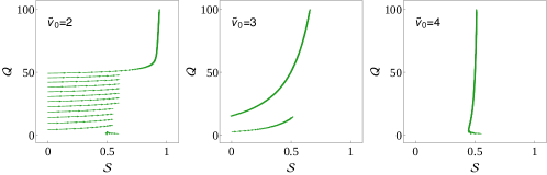
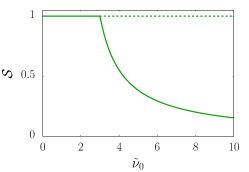
Figure 7: Critical learning rate for AdaTron learning. The first three plots from left to right are vector plots in phase space for the first-order system $(\dot{\mathcal{Q}},\dot{\mathcal{S}})$, Eq. (101), for AdaTron learning in the thermodynamic limit $N\to\infty$ with constant normalised learning rate $\tilde{\nu}(t)=\tilde{\nu}_{0}$ and $k=0.01$. For $\tilde{\nu}_{0}\leq 2$, there is an attracting state with $\mathcal{S}\to 1$. As we increase the learning rate $\tilde{\nu}_{0}$, another attracting state appears with $\mathcal{S}\to 1/2$ and hence $\epsilon=1/2$. In the limit $k\ll 1$, this behaviour can be understood from the bifurcation diagram of the closed, single equation for $\mathcal{S}$, Eq. (101b), shown on the far right, where stable (unstable) fixed points are indicated by straight (dashed) lines. Parameters: $\beta=D=1$.

The critical dependence of the generalisation error $\epsilon$ on the learning rate $\nu(t)=\sqrt{N}\tilde{\nu}_{0}$ for AdaTron learning in weak potentials ($k\ll 1$) in the thermodynamic limit $N\to\infty$ is most clearly seen by transforming variables from $(\mathcal{Q},\mathcal{R})$, Eq. (45), to $(\mathcal{Q},\mathcal{S})$ with

$$\mathcal{S}\equiv\frac{\mathcal{R}}{\sqrt{\mathcal{Q}}}.$$ (100)

The variables $(\mathcal{Q},\mathcal{S})$ obey another closed set of equations of motion. After averaging over the inputs using $p(x,y)$ as described in Section E, we find

$$\dot{\mathcal{Q}}(t)= 2+\mathcal{Q}(t)\left(-2k+(2\tilde{\nu}_{0}-\tilde{\nu}_{0}^{2})\frac{\mathcal{S}(t)\sqrt{1-\mathcal{S}(t)^{2}}-\arccos\mathcal{S}(t)}{\pi}\right),$$ (101a)

$$\dot{\mathcal{S}}(t)= -\frac{\mathcal{S}(t)}{\mathcal{\mathcal{Q}}(t)}+\frac{\tilde{\nu}_{0}^{2}\mathcal{S}(t)^{2}\sqrt{1-\mathcal{S}(t)^{2}}}{2\pi}+\frac{\tilde{\nu}_{0}\left(1-\mathcal{S}(t)^{2}\right)^{3/2}}{\pi}-\frac{\tilde{\nu}_{0}^{2}\mathcal{S}(t)\arccos\mathcal{S}(t)}{2\pi}.$$ (101b)

Three stream plots of this system for $\tilde{\nu}_{0}=2,3,4$, shown in Fig. 7, reveal a qualitative change in behaviour of the system ($\mathcal{Q},\mathcal{S}$) away from a solution with $\mathcal{S}\to 1$ and hence $\epsilon\to 0$. Indeed, as $\tilde{\nu}$ increases, $\mathcal{S}\to 0$ and thus $\epsilon\to 1/2$. This observation calls for a more detailed analysis of the system (101). Unfortunately, the fixed points of the system cannot be found explicitly. However, we can consider the limit of small $k$ where the transition is most pronounced, see Fig. 5. Expanding the equation for $\dot{\mathcal{Q}}(t)$ around $k=0$ and $\mathcal{S}=1$ shows that $\mathcal{Q}\sim 1/k$ in the steady state. This suggests neglecting the first term in Eq. (101b), which has the appealing consequence of yielding a closed, single equation for $\mathcal{S}(t)$. This equation has a fixed point $\mathcal{S}=1$, which is easily checked by substitution. Expanding Eq. (101b) around $\mathcal{S}=1$ yields

$$\dot{S}(t)=\frac{2\sqrt{2}}{\pi}\left(\frac{\tilde{\nu}_{0}^{2}}{3}-\tilde{\nu}_{0}\right)(1-\mathcal{S})^{3/2}+\mathcal{O}(1-\mathcal{S})^{5/2}$$ (102)

from which we see that the derivative will change sign at the critical learning rate $\tilde{\nu}_{c}=3$, which is the same value where the well-known breakdown of AdaTron learning occurs for a setup with $k=0$ and no thermal noise Engel and Van den Broeck (2001). A detailed graphical analysis (not shown) reveals that the solution $\mathcal{S}=1$ looses its stability at $\tilde{\nu}_{c}=3$ while a second fixed point emerges, which is stable, leading to the collapse of the generalisation error observed in Fig. 5. The bifurcation diagram for $\mathcal{S}$ is shown in the right-most plot of Fig. 7.

Appendix G Computing the excess heat

The most straightforward way to compute the excess heat for learning in the thermodynamic limit $N\to\infty$ after a quench of the learning rate to $\tilde{\nu}(t)=\tilde{\nu}_{0}$ is by relying on the machinery developed in Section E, namely the Itô stochastic differential equation for the weights, Eq. (86), which we rewrite slightly here as

$$\operatorname{d}\!{\bm{w}}=F(\bm{T},{\bm{w}},{\bm{\xi}})\operatorname{d}\!t+\operatorname{d}\!\mathbf{W}(t)$$ (103)

with the total force on the weights $F(\bm{T},{\bm{w}},{\bm{\xi}})$. The key insight here is due to K. Sekimoto, who realised that this equation is indeed a statement of the first law, with the stochastic heat increment defined as Sekimoto (1997, 2010)

$${\mathchar 22\relax\mkern-12.0mud}q\equiv F(\bm{T},{\bm{w}},{\bm{\xi}})\circ\operatorname{d}\!{\bm{w}}=\frac{1}{2}\left(F(\bm{T},{\bm{w}},{\bm{\xi}})+F(\bm{T},{\bm{w}}+\operatorname{d}\!{\bm{w}},{\bm{\xi}})\right)\operatorname{d}\!{\bm{w}}$$ (104)

where we have evaluated the stochastic product $\circ$ using the Stratonovich or mid-point convention for every component Gardiner (2009). For the excess heat, we replace the total force on the weights with the gradient of the “non-equilibrium” potential Seifert (2012)

$$\phi(\bm{T},{\bm{w}};\tilde{\nu}_{0})\equiv-\ln p^{\text{s}}(\bm{T},{\bm{w}};\tilde{\nu}_{0})$$ (105)

where $p^{\text{s}}(\bm{T},{\bm{w}};\tilde{\nu}_{0})$ is the steady-state distribution for $\tilde{\nu}_{0}$ with steady-state values $\mathcal{Q}^{\text{s}}(\tilde{\nu}_{0})$ and $\mathcal{R}^{\text{s}}(\tilde{\nu}_{0})$. Hence after averaging over the thermal noise, we find for the average increment in excess heat of the system over $N$

$${\mathchar 22\relax\mkern-12.0mud}Q^{\text{ex}}_{n}=\frac{1}{N}{\mathchar 22\relax\mkern-12.0mud}Q^{\text{ex}}\equiv -\frac{1}{N}\operatorname{d}\!{\bm{w}}\circ\nabla_{\bm{w}}\phi(\bm{T},{\bm{w}};\tilde{\nu}_{0})$$ (106)

$$= -\frac{1}{N}\operatorname{d}\!{\bm{w}}\circ\frac{{\bm{w}}-\mathcal{R}^{\text{s}}(\tilde{\nu}_{0})\bm{T}}{\mathcal{Q}^{\text{s}}(\tilde{\nu}_{0})-\mathcal{R}^{\text{s}}(\tilde{\nu}_{0})^{2}}$$ (107)

$$\begin{split}=&\frac{1}{\mathcal{Q}^{\text{s}}(\tilde{\nu}_{0})-\mathcal{R}^{\text{s}}(\tilde{\nu}_{0})^{2}}[k(\mathcal{Q}(t)-\mathcal{R}^{\text{s}}(\tilde{\nu}_{0})\mathcal{R}(t))-\tilde{\nu}_{0}\langle\operatorname{sgn}(x)y\mathcal{F}(x,y)\rangle\\[8.00003pt] &\qquad+\tilde{\nu}_{0}\mathcal{R}^{\text{s}}(\tilde{\nu}_{0})\langle\operatorname{sgn}(x)x\mathcal{F}(x,y)\rangle-\tilde{\nu}_{0}^{2}\langle\mathcal{F}(x,y)^{2}\rangle/2-1]\operatorname{d}\!t.\end{split}$$ (108)

where $\langle\cdot\rangle$ now indicates an average over the distribution $p(x,y)$ as described in Appendix E and we remind ourselves that we chose units where $D=1$.

References

- Berg and Purcell (1977) H. C. Berg and E. M. Purcell, Biophys. J. 20, 193 (1977).
- Seifert (2012) U. Seifert, Rep. Prog. Phys. 75, 126001 (2012).
- Parrondo et al. (2015) J. M. R. Parrondo, J. M. Horowitz, and T. Sagawa, Nat. Phys. 11, 131 (2015).
- Qian and Reluga (2005) H. Qian and T. C. Reluga, Phys. Rev. Lett. 94, 028101 (2005).
- Keymer et al. (2006) J. E. Keymer, R. G. Endres, M. Skoge, Y. Meir, and N. S. Wingreen, Proc. Natl. Acad. Sci. 103, 1786 (2006).
- Tu (2008) Y. Tu, Proc. Natl. Acad. Sci. U.S.A. 105, 11737 (2008).
- Endres and Wingreen (2009) R. G. Endres and N. S. Wingreen, Phys. Rev. Lett. 103, 158101 (2009).
- Lan et al. (2012) G. Lan, P. Sartori, S. Neumann, V. Sourjik, and Y. Tu, Nat. Phys. 8, 422 (2012).
- Mehta and Schwab (2012) P. Mehta and D. J. Schwab, Proc. Natl. Acad. Sci. U.S.A. 109, 17978 (2012).
- Skoge et al. (2013) M. Skoge, S. Naqvi, Y. Meir, and N. S. Wingreen, Phys. Rev. Lett. 110, 248102 (2013).
- Govern and ten Wolde (2014a) C. C. Govern and P. R. ten Wolde, Phys. Rev. Lett. 113, 258102 (2014a).
- Govern and ten Wolde (2014b) C. C. Govern and P. R. ten Wolde, Proc. Natl. Acad. Sci. U.S.A. 111, 17486 (2014b).
- Barato et al. (2014) A. C. Barato, D. Hartich, and U. Seifert, New J. Phys. 16, 103024 (2014).
- Lang et al. (2014) A. H. Lang, C. K. Fisher, T. Mora, and P. Mehta, Phys. Rev. Lett. 113, 148103 (2014).
- Sartori et al. (2014) P. Sartori, L. Granger, C. F. Lee, and J. M. Horowitz, PLoS Comput. Biol. 10, e1003974 (2014).
- Ito and Sagawa (2015) S. Ito and T. Sagawa, Nat. Commun. 6, 7498 (2015).
- ten Wolde et al. (2016) P. R. ten Wolde, N. B. Becker, T. E. Ouldridge, and A. Mugler, J. Stat. Phys. 162, 1395 (2016).
- Nishimori (2001) H. Nishimori, Statistical Physics of Spin Glasses and Information Processing, 1st ed. (Oxford University Press, Oxford, 2001) p. 252.
- Engel and Van den Broeck (2001) A. Engel and C. Van den Broeck, Statistical Mechanics of Learning (Cambridge University Press, 2001) p. 329.
- MacKay (2003) D. J. MacKay, Information Theory, Inference and Learning Algorithms (Cambridge University Press, 2003).
- Goldt and Seifert (2017) S. Goldt and U. Seifert, Phys. Rev. Lett. 118, 010601 (2017).
- Salazar (2017) D. S. P. Salazar, arxiv:1704.08724 (2017).
- Hebb (1949) D. O. Hebb, The organization of behavior: A neuropsychological approach (John Wiley & Sons, 1949).
- Vallet (1989) F. Vallet, EPL 8, 747 (1989).
- Rosenblatt (1962) F. Rosenblatt, Principles of Neurodynamics (Spartan, New York, 1962).
- Anlauf and Biehl (1989) J. K. Anlauf and M. Biehl, EPL 10, 687 (1989).
- Kandel et al. (2000) E. R. Kandel, J. H. Schwartz, T. M. Jessell, and Others, Principles of Neural Science (McGraw-Hill New York, 2000).
- Marr (1969) D. Marr, J. Physiol. 202, 437 (1969).
- Albus (1971) J. S. Albus, Math. Biosci. 10, 25 (1971).
- Ito and Kano (1982) M. Ito and M. Kano, Neurosci. Lett. 33, 253 (1982).
- Ito et al. (1982) M. Ito, M. Sakurai, and P. Tongroach, J. Physiol. 324, 113 (1982).
- Dayan and Abbott (2001) P. Dayan and L. F. Abbott, Theoretical Neuroscience (MIT Press, 2001).
- van Kampen (1992) N. van Kampen, Stochastic Processes in Physics and Chemistry (Elsevier, 1992) p. 465.
- Mace and Coolen (1998) C. W. H. Mace and A. C. C. Coolen, Stat. Comput. 8, 55 (1998).
- Note (1) We emphasise that the learning rate that we denote in this paper is an established concept in the analysis of neural networks and should not be confused with the learning rate Allahverdyan et al. (2009); Hartich et al. (2014) or the information flow Horowitz and Esposito (2014); Horowitz (2015) from stochastic thermodynamics which we use to prove our main result (see Appendix A). Here, we will use the term “thermodynamic learning rate” to refer to the latter.
- Hartich et al. (2014) D. Hartich, A. C. Barato, and U. Seifert, J. Stat. Mech. 2014, P02016 (2014).
- Horowitz (2015) J. M. Horowitz, J. Stat. Mech. 2015, P03006 (2015).
- Cover and Thomas (2006) T. M. Cover and J. A. Thomas, Elements of Information Theory (John Wiley & Sons, 2006) p. 748.
- Biehl and Riegler (1994) M. Biehl and P. Riegler, Europhys. Lett. 28, 525 (1994).
- Oono and Paniconi (1998) Y. Oono and M. Paniconi, Prog. Theor. Phys. Suppl. 130, 29 (1998).
- Van den Broeck and Esposito (2010) C. Van den Broeck and M. Esposito, Phys. Rev. E 82, 011144 (2010).
- Hatano and Sasa (2001) T. Hatano and S.-i. Sasa, Phys. Rev. Lett. 86, 3463 (2001).
- Heskes and Kappen (1991) T. M. Heskes and B. Kappen, Phys. Rev. A 44, 2718 (1991).
- Olver et al. (2010) F. Olver, D. Lozier, R. Boisvert, and C. Clark, eds., NIST Handbook of Mathematical Functions (Cambridge University Press, New York, NY, 2010).
- Minsky and Papert (1969) M. L. Minsky and S. A. Papert, Perceptrons (MIT Press, Cambridge MA, Cambridge, 1969).
- Barkai et al. (1995) N. Barkai, H. S. Seung, and H. Sompolinsky, Phys. Rev. Lett. 75, 1415 (1995).
- Gardner (1987) E. Gardner, EPL 4, 481 (1987).
- Polya (1954) G. Polya, Induction and Analogy in Mathematics (Princeton University Press, 1954).
- Cover (1965) T. M. Cover, IEEE Trans. Electron. Comput. EC-14, 326 (1965).
- Denker et al. (1987) J. Denker, D. Schwartz, B. Wittner, S. Solla, R. Howard, L. Jackel, and J. Hopfield, Complex Syst. s 1, 877 (1987).
- Cybenko (1989) G. Cybenko, Math. Control. Signals, Syst. 2, 303 (1989).
- Note (2) In both cases, the intermediate layer requires a sufficient number of neurons.
- Kinouchi and Caticha (1993) O. Kinouchi and N. Caticha, J. Phys. A. Math. Gen. 26, 6161 (1993).
- Biehl and Schwarze (1993) M. Biehl and H. Schwarze, J. Phys. A. Math. Gen. 26, 2651 (1993).
- Colabrese et al. (2017) S. Colabrese, K. Gustavsson, A. Celani, and L. Biferale, Phys. Rev. Lett. 118, 158004 (2017).
- Zdeborová and Krzakala (2016) L. Zdeborová and F. Krzakala, Adv. Phys. 65, 453 (2016).
- Allahverdyan et al. (2009) A. E. Allahverdyan, D. Janzing, and G. Mahler, J. Stat. Mech. 2009, P09011 (2009).
- Horowitz and Esposito (2014) J. M. Horowitz and M. Esposito, Phys. Rev. X 4, 031015 (2014).
- Jaynes (1957) E. T. Jaynes, Phys. Rev. 106, 620 (1957).
- Gardiner (2009) C. Gardiner, Stochastic Methods (Springer, Berlin-Heidelberg-New York-Tokyo, 2009) p. 447.
- Note (3) N.B. they use a different normalisation procedure from us.
- Sekimoto (1997) K. Sekimoto, J. Phys. Soc. Japan 66, 1234 (1997).
- Sekimoto (2010) K. Sekimoto, Stochastic Energetics, Lecture Notes in Physics, Vol. 799 (Springer Berlin Heidelberg, Berlin, Heidelberg, 2010).