Power-Based Direction-of-Arrival Estimation Using a Single Multi-Mode Antenna

Abstract

Phased antenna arrays are widely used for direction-of-arrival (DoA) estimation. For low-cost applications, signal power or received signal strength indicator (RSSI) based approaches can be an alternative. However, they usually require multiple antennas, a single antenna that can be rotated, or switchable antenna beams. In this paper we show how a multi-mode antenna (MMA) can be used for power-based DoA estimation. Only a single MMA is needed and neither rotation nor switching of antenna beams is required. We derive an estimation scheme as well as theoretical bounds and validate them through simulations. It is found that power-based DoA estimation with an MMA is feasible and accurate.

I Introduction

The state-of-the-art approach of DoA estimation relies on signal phase differences (assuming narrowband signals) between the elements of an antenna array [1]. DoA estimation methods are well known, however using an antenna array requires a complex receiver structure. For each array element, a separate receiver channel is required and the receiver channels have to be coherent and the system well calibrated. For low-cost applications, another possibility is to use signal power, i.e. RSSI measurements for DoA estimation. This requires knowledge of the antenna pattern and the possibility to cancel out or estimate the unknown path loss and transmit power of the signal.

In this paper we focus on power-based DoA estimation. Different techniques can be found in literature. One approach is to use an array of directional antennas pointing in different directions, see e.g. [2]. If only one antenna is available, an actuator can be used to rotate the antenna and thus obtain measurements from different angles. This approach may be used with either omnidirectional antennas having knowledge of the null in the pattern, see e.g. [3], or directional antennas, e.g. [4]. Instead of rotating the antenna, it is possible to make a controlled movement with the whole platform (e.g. a quadrocopter) [5]. Mechanical actuators have the drawback that they increase the power consumption of the system, possibly need maintenance and limit the update rate. Hence the authors in [6] avoid moving parts and propose a switched beam antenna. In general, high-resolution properties can be achieved with RSSI measurements. In [7], a variant of multiple signal characterization (MUSIC) suitable for signal power measurements is presented. The authors in [8] apply methods known from finite-rate-of-innovation (FRI) sampling to obtain high-resolution. All methods in the literature that the authors are aware of have in common that they either use multiple antennas or a single antenna with some sort of rotational movement or beams that require switching.

In contrast, this paper presents a power-based DoA estimation scheme with a MMA, which does not require any movement or switching of antenna beams. An MMA is in fact a single antenna element. Compared to antenna arrays, it has the advantage of being more compact, which can be important for applications with size constraints. The remainder of this paper is organised as follows. In Section II, the concept of the MMA is introduced. Section III quickly recapitulates the theoretical basis of this work termed wavefield modelling. The DoA estimation scheme is then developed in Section IV. The performance is evaluated in terms of theoretical bounds and simulations. Section V concludes the paper.

II Multi-Mode Antenna

In this section we provide a brief introduction to MMAs. The concept of MMAs is based on the theory of characteristic modes [9, 10]. This theory is available for more than 40 years, with significant amount of attention over the last 15 years. Recently the theory is more popular among antenna designers and is now known to be a useful design aid [11]. The main idea is to express the surface current distribution of conducting bodies as a sum of orthogonal functions called characteristic modes. These modes are independent of the excitation, i.e. they are defined by the shape and the size of the conductor. It is possible to determine modes numerically for antennas of arbitrary shape. For electrically small conductors, few modes are sufficient to describe the antenna behaviour [12]. Hence, electrically small conductors are well suited for an application of the theory of characteristic modes.

The idea of MMAs is to excite different characteristic modes independently. The current distribution for the particular mode, found by the theory of characteristic modes, defines the locations for excitation. In general, excitation is possible by inductive coupling at the current maxima, or by capacitive coupling at the respective minima [13]. The couplers belonging

to one mode are then connected to one port of the antenna. Due to the different modes being orthogonal to each other, MMAs are able to provide sufficient isolation of the ports [14].

Compared to classic antenna arrays MMAs are potentially more compact, which could be an advantage for applications with stringent size and weight constraints. The theory of characteristic modes provides a useful tool to design chassis antennas. For example, the case structure of a mobile handset device [15] or the platform of an unmanned aerial vehicle (UAV) can be used as antenna [16].

To the authors knowledge, MMAs have so far been investigated only for communication applications, see e.g. [17]. The aim of this paper is to show how their potential can be used for DoA estimation, enabling applications like localisation and orientation estimation. The antenna that we analyse in this paper has been proposed in [14]. Figure 1 shows the power pattern of this four port MMA for right hand circular polarisation (RHCP). The respective power pattern of the x-z plane is given in Figure 2. Obviously the antenna gain strongly depends on the incident angle of the signal. Moreover, the antenna patterns differ significantly between the four ports. Therefore the received signal power could be used to estimate the DoA of the signal. In the following, we assume that the polarisation of the received narrowband signal is purely RHCP.

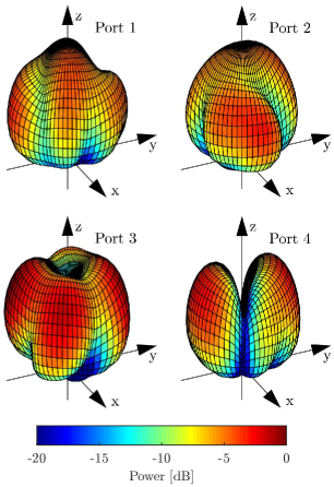
Figure 1: MMA power patterns for RHCP

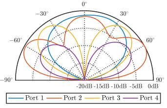
Figure 2: MMA x-z plane power patterns for RHCP

III Wavefield Modelling

The MMA is described in terms of spatial samples of the antenna power pattern obtained by electromagnetic field (EMF) simulation or calibration measurements. Since that representation might be relatively sparse, an interpolation strategy is needed, where we apply wavefield modelling and manifold separation [18]. In general, the manifold of the MMA is defined by $\theta\in[-\pi,\pi)$ for 2D and $\theta\in[0,\pi],\phi\in[0,2\pi)$ for the 3D case, where $\theta$ is the co-elevation and $\phi$ the azimuth. If a function is square integrable on this manifold, then it can be expanded in terms of an orthonormal basis. Hence the power pattern of an MMA with $M$ ports, $\bm{g}(\theta,\phi)\in\mathbb{R}^{M\times 1}$, can be decomposed [18], such that

$$\bm{g}(\theta,\phi)=\bm{G}\,\bm{\Psi}(\theta,\phi).$$ (1)

The matrix $\bm{G}\in\mathbb{R}^{M\times N}$ is called sampling matrix and $\bm{\Psi}(\theta,\phi)\in\mathbb{R}^{N\times 1}$ is the basis vector, with $N$ being the order of the basis. For 2D, the Fourier functions,

$$\bm{\Psi}(\theta)=\frac{1}{\sqrt{2\pi}}e^{j\bm{n}\theta},\>\bm{n}=[-N,...,N],$$ (2)

can be used as a basis. Then $\bm{G}_{m,N/2+1:N}=\bm{G}_{m,1:N/2}^{*}$, because $\bm{g}(\theta)$ must be real valued. For 3D we use the real spherical harmonic functions,

$$Y_{l}^{m}(\theta,\phi)=\begin{cases}\sqrt{2}N_{l}^{m}\cos(m\phi)P_{l}^{m}(\cos(\theta))&m>0\\ N_{l}^{0}P_{l}^{m}(\cos(\theta))&m=0\\ \sqrt{2}N_{l}^{|m|}\sin(|m|\phi)P_{l}^{|m|}(\cos(\theta))&m<0,\\ \end{cases}$$ (3)

with degree $l=0,...,L$ and order $m=-l,...,l$. $P_{l}^{m}(.)$ is the associated Legendre polynomial with degree $l$ and order $m$. The normalization factor $N_{l}^{m}$ is given by

$$N_{l}^{m}=\sqrt{\frac{2l+1}{4\pi}\frac{(l-m)!}{(l+m)!}}.$$ (4)

Using the enumeration $n=(l+1)l+m$, we can form an orthonormal basis,

$$\bm{\Psi}(\theta,\phi)=\bm{Y}_{\bm{n}}(\theta,\phi),\>\bm{n}=[0,...,N].$$ (5)

It is known that the magnitude of $\bm{G}$ decays superexponentially for $n\rightarrow\infty$ beyond $n=kr$, with $k$ being the angular wavenumber and $r$ the radius of the smallest sphere enclosing the antenna [18]. Figure 3 shows the magnitude of $\bm{G}$, i.e. the spherical harmonic coefficients, for the MMA. As can be seen, most of the energy is contained in the low order coefficients. Hence the expansion can be safely truncated at a certain order. As 1 is linear, having enough spatial samples of the antenna power pattern $\bm{\tilde{g}}(\theta,\phi)$ available from calibration measurements or EMF simulation, it is straightforward to determine the sampling matrix $\bm{G}$ for a given basis $\bm{\Psi}(\theta,\phi)$.

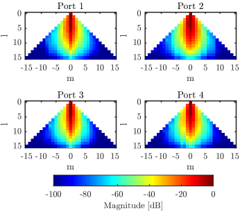
Figure 3: Magnitude of spherical harmonic coefficients, indices $l$ and $m$ are degree and order of the spherical harmonics in 3

Due to the assumption of narrowband and pure polarisation, it is sufficient to consider a scalar wavefield. Nevertheless, an extension to vector fields is possible [19]. Having a suitable model of the antenna at hand, we will now take a look at power-based DoA estimation.

IV Direction-of-Arrival Estimation

For simplicity, the derivations and simulations in Sections IV-A, IV-B, IV-C and IV-D focus on the 2D case, i.e. only a single angle $\theta$ is to be estimated. The extension to 3D and two angles of arrival follows in Section IV-E.

IV-A Signal Model

The received, sampled signal $r_{m}(k)$ at port $m$ of the MMA is given by

$$r_{m}(k)=a_{m}(\theta)s(k)+n_{m}(k)$$ (6)

where $k$ is the sample index, $a_{m}(\theta)$ is the attenuation caused by the antenna, $s(k)$ is the transmitted signal as it arrives at the receive antenna and $n_{m}(k)\sim\mathcal{CN}(0,\sigma^{2})$ is white circular symmetric normal distributed noise with variance $\sigma^{2}$. Assuming stationarity, the time-averaged received signal power over $K$ samples in time can be calculated by

$$\begin{split}\text{E}[P_{\mathrm{r},m}]&=\text{E}\left[\frac{1}{K}\sum_{k=1}^{K}|r_{m}(k)|^{2}\right]\\ &=\underbrace{|a_{m}(\theta,\phi)|^{2}}_{g_{m}(\theta,\phi)}\frac{1}{K}\sum_{k=1}^{K}|s(k)|^{2}+\text{E}\left[\frac{1}{K}\sum_{k=1}^{K}|n_{m}(k)|^{2}\right]\\ &=g_{m}(\theta,\phi)P_{\mathrm{s}}+\sigma^{2},\end{split}$$ (7)

with the antenna power pattern $g_{m}(\theta)$ and the signal power $P_{\text{s}}$. We follow an RSSI based approach, hence only power measurements are available to the receiver. The antenna power patterns, $\bm{g}(\theta)=[g_{1}(\theta),...,g_{M}(\theta)]$, are normalized such that $\max\bm{g}(\theta)=1$. The SNR for $g_{m}(\theta)=1$ is then given by

$$\text{SNR}=\frac{P_{\text{s}}}{\sigma^{2}}.$$ (8)

Defining $r_{m,\text{r}}(k)=\text{Re}[r_{m}(k)]$ and $r_{m,\text{i}}(k)=\text{Im}[r_{m}(k)]$, the sum of the squared magnitude of the received signal,

$$S_{\text{r},m}=\sum_{k=1}^{K}|r_{m}(k)|^{2}=\sum_{k=1}^{K}r_{m,\text{r}}^{2}(k)+r_{m,\text{i}}^{2}(k)\sim\chi^{2}(2K,\lambda,\sigma^{2}/2)$$ (9)

follows a noncentral $\chi^{2}$ distribution [20] with $2K$ degrees of freedom and noncentrality parameter

$$\begin{split}\lambda&=\sum_{k=1}^{K}\left(E[r_{m,\text{r}}(k)]^{2}+E[r_{m,\text{i}}(k)]^{2}\right)\\ &=\sum_{k=1}^{K}(a_{m}(\theta))^{2}(\text{Re}[s(k)]^{2}+\text{Im}[s(k)]^{2})\\ &=\sum_{k=1}^{K}g_{m}(\theta)|s(k)|^{2}\\ &=Kg_{m}(\theta)P_{\text{s}}.\end{split}$$ (10)

Its probability density function (PDF) is given by

$$p_{S_{\text{r},m}}(x)=\frac{1}{\sigma^{2}}\left(\frac{x}{\lambda}\right)^{\frac{K-1}{2}}e^{-\frac{\lambda+x}{\sigma^{2}}}I_{K-1}\left(\frac{2\sqrt{\lambda x}}{\sigma^{2}}\right),$$ (11)

with the modified Bessel function of the first kind $I_{\nu}(.)$. Since $P_{\text{r},m}$ is just a scaled version of that, its distribution can be obtained by transformation $p_{P_{\text{r},m}}(x)=Kp_{S_{\text{r},m}}(Kx)$. Inserting 10, we obtain

$$p_{P_{\text{r},m}}(x)=\frac{K}{\sigma^{2}}\left(\frac{x}{g_{m}(\theta)P_{\text{s}}}\right)^{\frac{K-1}{2}}e^{-\frac{K(g_{m}(\theta)P_{\text{s}}+x)}{\sigma^{2}}}\\ I_{K-1}\left(\frac{2K\sqrt{g_{m}(\theta)P_{\text{s}}x}}{\sigma^{2}}\right).$$ (12)

The mean and variance are given by

$$\begin{split}\tilde{\mu}_{m}&=\text{E}[P_{\text{r},m}]=K^{-1}\,\text{E}[S_{r,m}]\\ &=K^{-1}(K\sigma^{2}+\lambda)=g_{m}(\theta)P_{\text{s}}+\sigma^{2},\end{split}$$ (13)

$$\begin{split}\tilde{\sigma}_{m}^{2}&=\text{VAR}[P_{\text{r},m}]=K^{-2}\,\text{VAR}[S_{r,m}]\\ &=K^{-2}(K\sigma^{4}+2\sigma^{2}\lambda)\\ &=K^{-1}(\sigma^{4}+2g_{m}(\theta)P_{\text{s}}\sigma^{2}).\end{split}$$ (14)

For large $\lambda$ or large $K$, 12 is approximately Gaussian distributed $P_{\text{r},m}\sim\mathcal{N}(\tilde{\mu}_{m},\tilde{\sigma}_{m}^{2})$.

IV-B ML Estimator

The parameters to be estimated are given by

$$\bm{\Gamma}=[\theta,P_{\text{s}},\sigma^{2}].$$ (15)

We consider the case of unknown signal power $P_{\text{s}}$ and noise variance $\sigma^{2}$. Using the Gaussian approximation, i.e. $K$ is large, the log-likelihood function for the signal power measurements $\bm{P_{\text{r}}}=[P_{\text{r},1},...,P_{\text{r},M}]$ can be written as

$$\ln p(\bm{P_{\text{r}}};\bm{\Gamma})=\sum_{m=1}^{M}-\frac{1}{2}\ln(2\pi\tilde{\sigma}_{m}^{2})\\ -\frac{1}{2\tilde{\sigma}_{m}^{2}}\left(P_{\text{r},m}-(g_{m}(\theta)P_{\text{s}}+\sigma^{2})\right)^{2}.$$ (16)

The corresponding maximum likelihood (ML) estimator can then be derived as

$$\begin{split}\bm{\hat{\Gamma}_{\text{ML}}}&=\arg\max_{\bm{\Gamma}}\ln p(\bm{P_{r}};\bm{\Gamma})\\ &=\arg\min_{\bm{\Gamma}}\sum_{m=1}^{M}\ln\left(2\pi K^{-1}(\sigma^{4}+2g_{m}(\theta)P_{\text{s}}\sigma^{2})\right)\\ &\quad+\frac{K(P_{\text{r},m}-P_{\text{s}}g_{m}(\theta)-\sigma^{2})^{2}}{\sigma^{4}+2P_{\text{s}}g_{m}(\theta)\sigma^{2}}.\end{split}$$ (17)

A simplified version of the estimator,

$$\bm{\hat{\Gamma}_{\text{S}}}=\arg\min_{\bm{\Gamma}}\sum_{m=1}^{M}\frac{(P_{\text{r},m}-P_{\text{s}}g_{m}(\theta)-\sigma^{2})^{2}}{P_{\text{s}}g_{m}(\theta)+2\sigma^{2}},$$ (18)

can be obtained by neglecting the logarithmic term.

IV-C CRB Derivation

A lower bound on the variance of any unbiased estimator is the Cramér-Rao bound (CRB) [21]. For a given set of unknowns $\bm{\Gamma}=[\theta,P_{\text{s}},\sigma^{2}]$, it is defined as the inverse of the Fisher information matrix (FIM) $\bm{I}(\bm{\Gamma})$,

$$\text{VAR}[\bm{\hat{\Gamma}}]\geq\bm{I}(\bm{\Gamma})^{-1}.$$ (19)

Following the Gaussian assumption in 16, the elements of the FIM $\bm{I}(\bm{\Gamma})\in\mathbb{R}^{3\times 3}$ can be calculated as [21]

$$[\bm{I}(\Gamma)]_{i,j}=\sum_{m=1}^{M}\frac{1}{\tilde{\sigma}_{m}^{2}}\frac{\partial\tilde{\mu}_{m}}{\partial\Gamma_{i}}\frac{\partial\tilde{\mu}_{m}}{\partial\Gamma_{j}}+\frac{1}{2\tilde{\sigma}_{m}^{4}}\frac{\partial\tilde{\sigma}_{m}^{2}}{\partial\Gamma_{i}}\frac{\partial\tilde{\sigma}_{m}^{2}}{\partial\Gamma_{j}}.$$ (20)

Calculation of the partial derivatives of 13 and 14 requires the derivative of 1 and 2, which is given by

$$\frac{\partial\bm{g}(\theta)}{\partial\theta}=\bm{G}\frac{j\bm{n}}{\sqrt{2\pi}}e^{j\bm{n}\theta},\>\bm{n}=[-N,...,N].$$ (21)

Finally we obtain the CRB for the estimation of $\theta$,

$$\text{VAR}[\theta]\geq[\bm{I}(\bm{\Gamma})^{-1}]_{1,1}=\text{CRB}(\theta).$$ (22)

IV-D Simulation Results

In order to evaluate the feasibility of the proposed DoA estimation approach, we have used EMF simulation data of the MMA prototype, visualized in Figure 2. The simulated root-mean-square error (RMSE) and the CRB depending on $\theta$ are shown in Figure 4. The plot indicates that the achievable accuracy depends on the incident angle, with a RMSE spread of more than one order of magnitude over the manifold. Nevertheless, the ML estimator is able to attain the CRB for high signal-to-noise ratio (SNR).

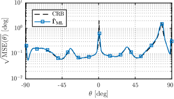
Figure 4: RMSE of the simulation and CRB for $\text{SNR}=20\,\mathrm{dB}$

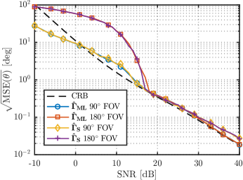
Figure 5: Simulated RMSE of ML and simplified estimator and CRB vs. SNR for full ($180^{\circ}$) and limited ($90^{\circ}$) FOV

In Figure 5 the mean over the manifold is plotted in dependence of the SNR present at the receiver. We have seen earlier, in Figure 2, that the antenna patterns are relatively symmetric around $0^{\circ}$. For that reason, we compare the performance with a limited field of view (FOV) of $90^{\circ}$ to the full FOV of $180^{\circ}$. It can be seen that for $\text{SNR}\geq 18\,\mathrm{dB}$, the ML estimator $\bm{\hat{\Gamma}_{\text{ML}}}$ defined in 17 is efficient, i.e. it attains the CRB. For lower SNR, the RMSE is significantly bigger for $180^{\circ}$ due to ambiguities caused by the antenna pattern. The CRB is calculated independent of the a-priori information regarding FOV limitation, hence it is not an accurate lower bound in the low SNR region. Finally the plot indicates that the simplified estimator $\bm{\hat{\Gamma}_{\text{S}}}$ given by 18 is sufficiently accurate. Only for high SNR, a slight increase in RMSE compared to the ML estimator is visible.

IV-E Extension to 3D

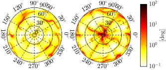
Figure 6: $\sqrt{CRB(\theta)}$ (left) and $\sqrt{CRB(\phi)}$ (right) for $\text{SNR}=20\,\mathrm{dB}$

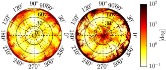
Figure 7: $\sqrt{MSE(\theta)}$ (left) and $\sqrt{MSE(\phi)}$ (right) for $\text{SNR}=20\,\mathrm{dB}$

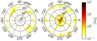
Figure 8: $\sqrt{CRB(\theta)}$ (left) and $\sqrt{CRB(\phi)}$ (right) for $\text{SNR}=30\,\mathrm{dB}$

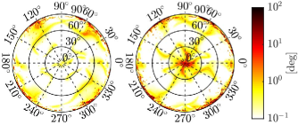
Figure 9: $\sqrt{MSE(\theta)}$ (left) and $\sqrt{MSE(\phi)}$ (right) for $\text{SNR}=30\,\mathrm{dB}$

Having studied the performance in 2D, we now extend the proposed DoA estimation scheme to the more practical case of 3D, i.e. two unknown angles of arrival. The extension of the signal model to 3D,

$$r_{m}(k)=a_{m}(\theta,\phi)s(k)+n_{m}(k),$$ (23)

is straight forward. One more parameter, $\phi$, has to be estimated, so we have $\bm{\Gamma}=[\theta,\phi,P_{\text{s}},\sigma^{2}]$. The FIM then grows to $I(\bm{\Gamma})\in\mathbb{R}^{4\times 4}$. Applying wavefield modelling with spherical harmonics as described in Section III, the partial derivatives of the antenna power pattern are

$$\frac{\partial\bm{g}(\theta,\phi)}{\partial\theta}=\bm{G}\frac{\partial}{\partial\theta}Y_{n}(\theta,\phi),$$ (24a)

$$\frac{\partial\bm{g}(\theta,\phi)}{\partial\phi}=\bm{G}\frac{\partial}{\partial\phi}Y_{n}(\theta,\phi),$$ (24b)

using the enumeration $n=(l+1)l+m$. The partial derivative of 3 with respect to $\theta$ (for $\theta\neq 0$) is given by

$$\frac{\partial}{\partial\theta}Y_{l}^{m}(\theta,\phi)=\begin{cases}\sqrt{2}N_{l}^{m}\cos(m\phi)\frac{\partial P_{l}^{m}(\cos(\theta))}{\partial\theta}&m>0\\ N_{l}^{0}\frac{\partial P_{l}^{m}(\cos(\theta))}{\partial\theta}&m=0\\ \sqrt{2}N_{l}^{|m|}\sin(|m|\phi)\frac{\partial P_{l}^{|m|}(\cos(\theta))}{\partial\theta}&m<0.\\ \end{cases}$$ (25)

The derivative of the Legendre polynomial $P_{l}^{m}(\cos(\theta))$,

$$\frac{\partial P_{l}^{m}(\cos(\theta))}{\partial\theta}=\frac{1+l-m}{\sin(\theta)}P_{l+1}^{m}(cos(\theta))-\frac{l+1}{\tan(\theta)}P_{l}^{m}(\cos(\theta)),$$ (26)

can be calculated with the help of [22]. The corresponding partial derivative of 3 with respect to $\phi$ is given by

$$\frac{\partial}{\partial\phi}Y_{l}^{m}(\theta,\phi)=\begin{cases}\sqrt{2}N_{l}^{m}(-m)\sin(m\phi)P_{l}^{m}(\cos(\theta))&m>0\\ 0&m=0\\ \sqrt{2}N_{l}^{|m|}(-m)\cos(m\phi)P_{l}^{|m|}(\cos(\theta))&m<0.\\ \end{cases}$$ (27)

Finally we obtain the CRBs for the estimation of $\theta$ and $\phi$ in the 3D case,

$$\text{VAR}[\hat{\theta}]\geq[\bm{I}(\bm{\Gamma})^{-1}]_{1,1}=\text{CRB}(\theta),$$ (28a)

$$\text{VAR}[\hat{\phi}]\geq[\bm{I}(\bm{\Gamma})^{-1}]_{2,2}=\text{CRB}(\phi).$$ (28b)

In order to confirm the expected DoA estimation performance, we performed simulations for the 3D case. Figure 6 shows the CRB in $\theta$- and $\phi$-domain for $\text{SNR}=20\,\mathrm{dB}$. The corresponding simulation result can be seen in Figure 7. Apparently, the CRB is not attained on the whole manifold. Especially for low elevations, an excessive estimation error can be observed. Taking another look at the antenna power pattern in Figure 1, it is obvious that at low elevations the antenna gain is very small. This leads to a degradation of the DoA estimation performance. For mid and high elevations, the CRB is usually attained, except for a few directions which appear as dark dots in Figure 7. This is most likely caused by estimation ambiguities due to the symmetry of the antenna pattern. In practice a-priori information, i.e. a rough knowledge of the direction, is often available, which may help to solve the ambiguity. Next we take a look at Figures 8 and 9 showing the CRB and simulation RMSE at $\text{SNR}=30\,\mathrm{dB}$. To allow comparison, Figures 6, 7, 8 and 9 use the same scaling. It can be seen that by increasing the SNR by $10\,\mathrm{dB}$, both perturbing effects, i.e. low gain at low elevation angles and estimation ambiguities, are strongly reduced. Only for low elevations, an increased error can still be observed. The higher RMSE at high elevation for the $\phi$-domain is less problematic, since at the pole this translates to a smaller directional error.

V Conclusion

A suitable model for MMAs, building on the concept of wavefield modelling, was introduced. Based on that model, a power-based maximum likelihood DoA estimation scheme has been introduced. Simulations have shown that in general, power-based DoA estimation with MMAs is feasible. However, for certain incident angles, ambiguities in the antenna pattern cause an increased estimation variance. For the investigated MMA prototype, low elevations are problematic due to low antenna gain. Altogether it can be concluded that power-based DoA estimation is possible with MMAs, but for accurate estimates a relatively high SNR is required. Further work will be performed by using signal polarisations as well as investigations into coherent receivers, that are able to obtain phase information from the different ports of the MMA.

References

- [1] T. E. Tuncer and B. Friedlander, Classical and Modern Direction-of-Arrival Estimation. Academic Press, Jul. 2009.
- [2] J. Ash and L. Potter, “Sensor network localization via received signal strength measurements with directional antennas,” in Proceedings of the 2004 Allerton Conference on Communication, Control, and Computing, 2004, pp. 1861–1870.
- [3] M. Malajner, P. Planinsic, and D. Gleich, “Angle of Arrival Estimation Using RSSI and Omnidirectional Rotatable Antennas,” IEEE Sensors Journal, vol. 12, no. 6, pp. 1950–1957, Jun. 2012.
- [4] B. N. Hood and P. Barooah, “Estimating DoA From Radio-Frequency RSSI Measurements Using an Actuated Reflector,” IEEE Sensors Journal, vol. 11, no. 2, pp. 413–417, Feb. 2011.
- [5] J. T. Isaacs, F. Quitin, L. R. G. Carrillo, U. Madhow, and J. P. Hespanha, “Quadrotor control for RF source localization and tracking,” in 2014 International Conference on Unmanned Aircraft Systems (ICUAS), May 2014, pp. 244–252.
- [6] A. Cidronali, S. Maddio, G. Giorgetti, and G. Manes, “Analysis and Performance of a Smart Antenna for 2.45-GHz Single-Anchor Indoor Positioning,” IEEE Transactions on Microwave Theory and Techniques, vol. 58, no. 1, pp. 21–31, Jan. 2010.
- [7] M. Passafiume, S. Maddio, A. Cidronali, and G. Manes, “MUSIC algorithm for RSSI-based DoA estimation on standard IEEE 802.11/802.15. x systems,” WSEAS Trans. Signal Process., vol. 11, pp. 58–68, 2015.
- [8] J. P. Lie, T. Blu, and C. M. S. See, “Single Antenna Power Measurements Based Direction Finding,” IEEE Transactions on Signal Processing, vol. 58, no. 11, pp. 5682–5692, Nov. 2010.
- [9] R. Garbacz and R. Turpin, “A generalized expansion for radiated and scattered fields,” IEEE Transactions on Antennas and Propagation, vol. 19, no. 3, pp. 348–358, 1971.
- [10] R. Harrington and J. Mautz, “Theory of characteristic modes for conducting bodies,” IEEE Transactions on Antennas and Propagation, vol. 19, no. 5, pp. 622–628, 1971.
- [11] B. K. Lau, D. Manteuffel, H. Arai, and S. V. Hum, “Guest Editorial Theory and Applications of Characteristic Modes,” IEEE Transactions on Antennas and Propagation, vol. 64, no. 7, pp. 2590–2594, Jul. 2016.
- [12] M. Cabedo-Fabres, E. Antonino-Daviu, A. Valero-Nogueira, and M. F. Bataller, “The theory of characteristic modes revisited: A contribution to the design of antennas for modern applications,” IEEE Antennas and Propagation Magazine, vol. 49, no. 5, pp. 52–68, 2007.
- [13] R. Martens, E. Safin, and D. Manteuffel, “Inductive and capacitive excitation of the characteristic modes of small terminals,” in Antennas and Propagation Conference (LAPC), 2011 Loughborough. IEEE, 2011, pp. 1–4.
- [14] D. Manteuffel and R. Martens, “Compact Multimode Multielement Antenna for Indoor UWB Massive MIMO,” IEEE Transactions on Antennas and Propagation, vol. 64, no. 7, pp. 2689–2697, Jul. 2016.
- [15] H. Li, Y. Tan, B. K. Lau, Z. Ying, and S. He, “Characteristic Mode Based Tradeoff Analysis of Antenna-Chassis Interactions for Multiple Antenna Terminals,” IEEE Transactions on Antennas and Propagation, vol. 60, no. 2, pp. 490–502, Feb. 2012.
- [16] Y. Chen and C. F. Wang, “Electrically Small UAV Antenna Design Using Characteristic Modes,” IEEE Transactions on Antennas and Propagation, vol. 62, no. 2, pp. 535–545, Feb. 2014.
- [17] P. A. Hoeher and N. Doose, “A massive MIMO terminal concept based on small-size multi-mode antennas,” Transactions on Emerging Telecommunications Technologies, p. e2934, Mar. 2015.
- [18] M. A. Doron and E. Doron, “Wavefield modeling and array processing. I. Spatial sampling,” IEEE Transactions on Signal Processing, vol. 42, no. 10, pp. 2549–2559, 1994.
- [19] M. Costa, A. Richter, and V. Koivunen, “DoA and Polarization Estimation for Arbitrary Array Configurations,” IEEE Transactions on Signal Processing, vol. 60, no. 5, pp. 2330–2343, May 2012.
- [20] J. G. Proakis and M. Salehi, Digital Communications, 5th ed. Boston, Mass.: McGraw-Hill, 2008.
- [21] S. M. Kay, Fundamentals of Statistical Signal Processing, Volume I: Estimation Theory, 1st ed. Englewood Cliffs, N.J: Prentice Hall, Apr. 1993.
- [22] F. W. J. Olver and National Institute of Standards and Technology (U.S.), Eds., NIST Handbook of Mathematical Functions. Cambridge; New York: Cambridge University Press : NIST, 2010.