X-shooter spectroscopy of young stellar objects in Lupus:

Abstract

Aims. With the purpose of performing a homogeneous determination of elemental abundances for members of the Lupus T association, we analyzed three chemical elements: lithium, iron, and barium. The aims were: 1) to derive the lithium abundance for the almost complete sample ($\sim 90\%$) of known class II stars in the Lupus I, II, III, and IV clouds; 2) to perform chemical tagging of a region where few iron abundance measurements have been obtained in the past, and no determination of the barium content has been done up to now. We also investigated possible barium enhancement at the very young age of the region, as this element has become increasingly interesting in the last few years following the evidence of barium over-abundance in young clusters, the origin of which is still unknown.

Methods. Using the X-shooter spectrograph mounted on the Unit 2 (UT2) at the Very Large Telescope (VLT), we analyzed the spectra of 89 cluster members, both class II (82) and class III (7) stars. We measured the strength of the lithium line at $\lambda$6707.8 Å and derived the abundance of this element through equivalent width measurements and curves of growth. For six class II stars we also derived the iron and barium abundances using the spectral synthesis method and the code MOOG. The veiling contribution was taken into account in the abundance analysis for all three elements.

Results. We find a dispersion in the strength of the lithium line at low effective temperatures and identify three targets with severe Li depletion. The nuclear age inferred for these highly lithium-depleted stars is around $15$ Myr, which exceeds by an order of magnitude the isochronal one. We derive a nearly solar metallicity for the members whose spectra could be analyzed. We find that Ba is over-abundant by $\sim 0.7$ dex with respect to the Sun. Since current theoretical models cannot reproduce this abundance pattern, we investigated whether this unusually large Ba content might be related to effects due to stellar parameters, stellar activity, and accretion.

Conclusions. We are unable to firmly assess whether the dispersion in the lithium content we observe is a consequence of an age spread. As in other star-forming regions, no metal-rich members are found in Lupus, giving support to a recent hypothesis that the iron abundance distribution of most of the nearby young regions could be the result of a common and widespread star formation episode involving the Galactic thin disk. Among the possible causes or sources for Ba enhancement examined here, none is sufficient to account for the over-abundance of this element at a $\sim 0.7$ dex level..

1 Introduction

The determination of elemental abundances in nearby ($<$ $500$ pc) star-forming regions (SFRs) is important for a variety of astrophysical problems, in both exo-planetary and stellar contexts. The members of these regions are still close to their birthplace. Their elemental abundances are thus fundamental to trace the present chemical pattern of the Galactic thin disk in the solar neighborhood and the interstellar medium in which they are immersed.

In the last three decades, an increasing number of studies have focused on the abundance measurements of iron and other elements in SFRs, young clusters, and associations, and specifically in their low-mass members (e.g., Padgett 1996; Cunha et al. 1998; James et al. 2006; Santos et al. 2008; González-Hernández et al. 2008; Viana Almeida et al. 2009; D’Orazi & Randich 2009; Biazzo et al. 2011a, b; D’Orazi et al. 2011; Tabernero et al. 2012; Biazzo et al. 2012a, b; Spina et al. 2014a, b). In particular, three elements have gradually been more analyzed in studies investigating the chemical pattern of young regions, namely lithium (Li), iron (Fe), and barium (Ba).

Lithium is a fragile element, which is burnt at temperatures of $\sim 3\times 10^{6}$ K (see, e.g., Bildsten et al. 1997). Temperatures of this order can be easily reached in the interior of a low-mass pre-main sequence (PMS) star as it contracts towards the main sequence (Bodenheimer et al. 1965). Therefore, low-mass stars ($\sim 0.05-0.7\,M_{\odot}$) deplete their initial Li content during the PMS phase; the depletion timescale depends on stellar mass, with stars of $\sim 0.7-0.2\,M_{\odot}$ starting to burn it after $\sim 2-15$ Myr and stars of $<0.2\,M_{\odot}$ after $\sim 20-25$ Myr (see Baraffe et al. 2015, and references therein). Therefore, lithium abundance has been widely used as an independent and reliable method to estimate the ages of low-mass members of young regions (see, e.g., Song et al. 2002; White & Hillenbrand 2005; Palla et al. 2005, 2007; Sacco et al. 2007; Yee & Jensen 2010; Sergison et al. 2013; Lim et al. 2016).

The determination of the abundance of iron, iron-peak, and alpha elements is important in the field of star formation. In fact, several studies have provided hints that regions where star formation has ceased generally share a metallicity close to the solar value, while SFRs where the molecular gas is still present seem to be characterized by a slightly lower iron content (Biazzo et al. 2011a; Spina et al. 2014b, and references therein). Whether this is due to low-number statistics (both in regions and in number of analyzed targets per region) or inhomogeneous and uncertain methodologies is still debated. Spina et al. (2014b) recently claimed that the metal-poor nature of these young environments could be the result of a common and widespread star formation episode involving the Gould Belt, and giving birth to most of the SFRs, and stars in the solar neighborhood (see also Guillout et al. 1998). However, the possibility of a more complex process of chemical evolution that involved a much larger area in the disk of the Milky Way Galaxy is not excluded (Spina et al. 2017).

Barium is synthesized by neutron capture reactions mostly by the so called $s$-process occurring in asymptotic giant branch (AGB) stars and represents an excellent tracer of chemical enrichment mechanisms in the Galaxy; for this reason, many studies have been focused on deriving barium abundance in both field stars in the halo and thick/thin disk, and in stellar clusters older than $\sim$100 Myr. Fewer studies are available for young clusters and associations, while to our knowledge no determination of barium abundance for late-type members of SFRs exists to date. D’Orazi et al. (2009) detected a trend of increasing [Ba/Fe] with decreasing age from roughly solar abundance up to $\sim 0.3$ dex for open clusters in the age range $\sim 0.5-4.5$ Gyr. D’Orazi et al. (2009) reproduced such behavior by assuming higher Ba yields from low-mass AGB stars in their Galactic chemical evolution models (see also Maiorca et al. 2014). A further increase in still younger clusters, up to $\sim 0.6-0.7$ dex at $\sim 35$ Myr, was also found by D’Orazi et al. (2009); this behavior is not reproduced by the same models. They argued that a process creating Ba in the last dozen Myr through Galactic chemical evolution is quite unlikely, unless local enrichment is invoked. Other recent studies confirmed the presence of high Ba abundance in $\sim 30-50$ Myr old stars (Desidera et al. 2011; D’Orazi et al. 2012). Several hypotheses (high level of chromospheric activity, uncertainty in stellar parameters, effects of the stratification in temperature of the model atmosphere, non local thermodynamic equilibrium, NLTE, corrections) were proposed to reproduce the high Ba content in young clusters, but all of them failed in explaining the observed over-abundance.

Here, we present a systematic and homogeneous analysis of elemental abundances of PMS stars in the Lupus cloud complex. Lupus is one of the most nearby ($d\sim 150-200$ pc) and largest low-mass star-forming regions (see Comerón (2008) for a review). Similarly to other regions (e.g., Taurus, Chamaeleon, Ophiucus, Corona Australis), a large variety of objects in various stages of evolution are present in Lupus. The region of the sky occupied by the Lupus clouds is almost devoid of early-type stars and shows no sign of ongoing high-mass star forming activity, although the large number of OB members of the Scorpius-Centaurus SFR in the vicinity of the Lupus complex implies the existence of an ambient field of high energy sources, which are likely to have played an important role in the evolution and possibly the origin of the Lupus complex (Tachihara et al. 2001). This makes the Lupus stellar population of particular interest for comparative studies with other nearby regions, such as Taurus-Auriga and Chamaeleon, which have a similar mass of molecular gas and low-mass star formation activity, but which evolved more in isolation and relatively unperturbed (Comerón 2008).

This is a companion paper to previous studies focused on the investigation of the accretion properties of Lupus PMS stars (Alcalá et al. 2014, 2017), as well as the determination of their stellar parameters and activity indicators (Frasca et al. 2017). We used the same data as in those works, namely spectra acquired with the X-shooter spectrograph on the Very Large Telescope (VLT; Paranal, Chile), in order to study the abundance of lithium, iron, and barium of the low-mass ($\sim 0.025-1.8\,M_{\odot}$) PMS stars in Lupus. While a few studies of elemental abundance of iron, silicon, and nickel in a handful of class III stars in this region have been performed in the past (see, Santos et al. 2008, and references therein), and only one class II was analyzed in terms of iron abundance (Padgett 1996), a homogeneous and self-consistent analysis of Li, Fe, and Ba in a significant sample of the class II sources is still lacking. In this paper, we aim to cover this gap.

The outline of this paper is as follows. The data sample is presented in Sect. 2. In Sect. 3, we derive the elemental abundances of lithium, iron, and barium. We then discuss the implications of our findings in Sect. 4. In Sect. 5 a summary of our results is presented.

2 Data set

The data set for this paper is exactly the same as in our previous works (Alcalá et al. 2014, 2017; Frasca et al. 2017). All the criteria for the target selection, as well as observational strategy, are provided in those papers. We adopt the same listing order as in Frasca et al. (2017) in our Table 1.

The final sample includes 82 class II and seven class III sources in Lupus clouds I, II, III, and IV. Forty-three objects were observed in 2010-2012 during the INAF (Istituto Nazionale di Astrofisica) guaranteed time observations (GTO; Alcalá et al. 2011, 2014), forty sources were observed in 2015 and 2016 during the ESO (European Southern Observatory) periods 95 and 97, and the remaining six were taken from the ESO archive (see Alcalá et al. 2017; Frasca et al. 2017). All targets were observed using the 0$\aas@@fstack{\prime\prime}$9 slit at a resolution of $R\sim 8\,800$ in the VIS (visible) arm, with the exception of four (Sz 68, Sz 74, Sz 83, and Sz 102) in P95 and P97, and those of the ESO archive, which were observed using the 0$\aas@@fstack{\prime\prime}$4 VIS slit at a resolving power of $R\sim 17\,400$. The sample comprises 82 class II and seven class III sources. For details about data reduction, observing log-book, and selection criteria, we refer to Alcalá et al. (2014, 2017) and Manara et al. (2013). Throughout this paper, stellar parameters (effective temperature $T_{\rm eff}$, surface gravity $\log g$, projected rotational velocity $v\sin i$, veiling $r$) and membership information (radial velocity $v_{\rm rad}$) were taken from Frasca et al. (2017), while spectral types were taken from Alcalá et al. (2017) and Manara et al. (2013). The sample of class II objects in the aforementioned Lupus clouds is complete at more than $\sim 90$% level (Alcalá et al. 2017).

3 Analysis

Lithium abundances were measured from the line equivalent widths and by using appropriate curves of growth (Sect. 3.1.2), while iron and barium abundances were determined through the spectral synthesis method and the synth driver within the MOOG code (Sneden 1973; see Sect. 3.2). This is the most adequate strategy to derive the abundances, given the relatively low resolution of our spectra.

3.1 The lithium line

3.1.1 Equivalent widths

Equivalent widths of the lithium line ($EW_{\rm Li}$) at $\lambda=6707.8$ Å  were measured by direct integration or by Gaussian fit using the IRAF task splot. At the X-shooter resolution the Li i line is blended with the Fe i $\lambda$ 6707.4 Å line, whose contribution was subtracted using the empirical correction between $EW_{\rm Fe}$ and the $B-V$ color by Soderblom et al. (1993). To estimate the correction, we considered the $T_{\rm eff}$ determinations by Frasca et al. (2017) and the calibration by Pecaut & Mamajek (2013). For stars cooler than 4000 K, the real continuum is no longer visible, due to the increasing strength of molecular bands. Therefore, the lithium equivalent widths are referred to the local pseudo-continuum, and the molecular bands are the major blending sources. However, we integrated the lithium line including the blends, as in Palla et al. (2007) to be consistent with their curves of growth (see Sect. 3.1.2).

Errors in $EW_{\rm Li}$ were evaluated by determining the signal-to-noise ($S/N$) ratio at wavelengths adjacent to the lithium line and by multiplying its reciprocal by the width of the integration range. Typical errors in lithium equivalent widths are of 20-25 mÅ (see Table 1).

Our spectra are affected by spectral veiling ($r$), that is, the amount of continuum excess emission, which fills in the lines. Measured $EW_{\rm Li}$ were corrected for this contribution using the $r$ values expressed in units of the photospheric continuum and determined by Frasca et al. (2017) in several spectral regions. We applied the relationship $EW_{\rm Li}^{\rm corr}=EW_{\rm Li}(1+r)$, where $EW_{\rm Li}^{\rm corr}$ is the corrected value for the lithium equivalent width. For the Li i line at $\lambda=6707.8$ Å, we adopted the mean value ($r_{6700}$) between $\lambda=6200$ Å and $\lambda=7100$ Å (see Table 1). As in Frasca et al. (2017), all values of veiling $\leq 0.2$ are considered non detectable and set equal to zero. This is the case of about 65% of the targets, while, for the rest of the sample, $r_{6700}$ ranges from $\sim 0.3$ up to $\sim 3$. Figure 1 shows the $EW_{\rm Li}$ versus $T_{\rm eff}$ plot for the 89 Lupus members listed in Table 1, as obtained from our measurements and after the correction both for the blending with the iron line and the veiling contribution as explained above. The distribution of the corrected equivalent width peaks at $\sim 560$ mÅ (see also Fig. 2), with most of the spread at a given $T_{\rm eff}$ reduced after the aforementioned corrections. The residual scatter in $EW_{\rm Li}^{\rm corr}$ could be due to measurement errors, but we cannot exclude the possibility that part of the dispersion may be due to stars with Li depletion. For five targets (Lup 706, Par-Lup3-4, 2MASS J16085953-3856275, SSTc2d J154508.9-341734, and 2MASS J16085373-3914367) we were not able to measure $EW_{\rm Li}$ because of low $S/N$ and/or high veiling contribution. However, the lithium content of these objects is below the level of other stars with similar effective temperature. For one target (Sz 94) we did not detect the line (see Table 1 and discussion in Sect. 4.1). We consider these six targets as upper limits, since the error in equivalent width is larger than the $EW_{\rm Li}$ value. The rest of the targets with low lithium content ($EW_{\rm Li}^{\rm corr}\raisebox{-2.15277pt}{$\>\stackrel{{\scriptstyle\textstyle<}}{{\sim}}\>$}200$ mÅ) have negligible veiling ($r_{6700}\raisebox{-2.15277pt}{$\>\stackrel{{\scriptstyle\textstyle<}}{{\sim}}\>$}0.2$) and suggest a possible large amount of Li depletion. They will be discussed in Sect. 4.1.

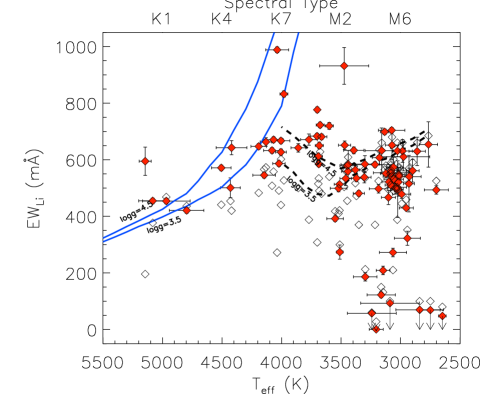
Figure 1: Lithium equivalent width versus effective temperature for the studied sample. Open symbols refer to measured $EW_{\rm Li}$, while filled red symbols represent the lithium equivalent widths after correction for blending with the iron line and spectral veiling. Overplotted as black dashed and blue solid lines are the COGs at $\log g=3.5,4.5$ and lithium abundance of 3.5 dex from Palla et al. (2007) and Pavlenko & Magazzù (1996), respectively. Arrows indicate upper limits (see text). Spectral types as in Luhman et al. (2003) for M-type young stellar objects (YSOs) and Kenyon & Hartmann (1995) for K-type YSOs are also marked (see also Alcalá et al. 2017 and Table 1).

Figure 2 shows the position of all members in an $EW_{\rm Li}^{\rm corr}$ versus radial velocity (RV) plot, where RVs by Frasca et al. (2017) were transformed to the local standard of rest (LSR). In the same plot, the RV distribution of the gas derived by Vilas-Boas et al. (2000) from the ¹³CO ($J=1-0$) transition in 35 dense molecular cores in Lupus I, II, III, and IV is shown. Our RV distribution is in good agreement, within the errors, with the average velocity of the gas, that is, $<V_{\rm LSR}>_{\rm gas}=4.7\pm 0.3$ km/s, as also found in other regions (Biazzo et al. 2012a; Da Rio et al. 2017). All but six stars (Sz 66, Sz 91, SSTc2d160901.4-392512, Sz 123A, Sz 102, and Sz 122) are confined inside $\pm 2\sigma$ from the peak at 9.6 km/s of the RV distribution, where $\sigma=5.4$ km/s. The six stars outside the $<V_{\rm LSR}>\pm 2\sigma$ distribution could be spectroscopic binaries because both their high lithium content and proper motions (Girard et al. 2011; López Martí et al. 2011) strongly suggest membership. Five of them have large $EW_{\rm Li}^{\rm corr}$, which gives support to their membership to the Lupus SFR. One of these, Sz 102, shows a large $V_{\rm LSR}$ error, maybe due to the high $v\sin i$ and veiling (see Frasca et al. 2017). The star with low $EW_{\rm Li}^{\rm corr}$ and outside the $<V_{\rm LSR}>\pm 2\sigma$ distribution is Sz 122, a class III object with $v\sin i\sim 150$ km/s. This high-rotational velocity target is suspected to be a spectroscopic binary, as reported by Stelzer et al. (2013).

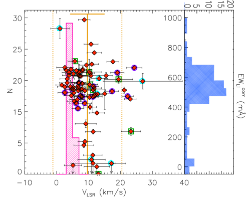
Figure 2: Corrected lithium equivalent width versus radial velocity (from Frasca et al. 2017) in the LSR. Different symbols are used for class III (open green squares), transitional disk (violet circles), and sub-luminous or flat spectral energy distribution objects (cyano pentagons), as defined in Alcalá et al. (2017). The vertical solid line indicates the mean $V_{\rm LSR}$ ($9.6\pm 5.4$ km/s) of our targets, while the dotted ones represent the $<V_{\rm LSR}>\pm 2\sigma$ values. Upper limits are marked by arrows. The magenta hatched histogram in the background of the central panel represents the velocity distribution of gas condensations in Lupus as derived by Vilas-Boas et al. (2000). The histogram on the right panel shows our $EW_{\rm Li}$ distribution, with a peak around $\sim 560$ mÅ.

3.1.2 Elemental abundances

Lithium abundances, $A$(Li), were estimated from the $EW_{\rm Li}^{\rm corr}$ measured in this work, the atmospheric parameters ($T_{\rm eff}$, $\log g$) taken from Frasca et al. (2017), and using the NLTE curves of growth (COGs) reported by Pavlenko & Magazzù (1996) for $T_{\rm eff}>4000$ K, the COGs by Palla et al. (2007) for $T_{\rm eff}<3500$ K, and the average of these COGs for $3500<T_{\rm eff}<4000$ K. The main source of error in $A{\rm(Li)}$ comes from the uncertainty in stellar parameters ($T_{\rm eff}$ and $\log g$), listed in Frasca et al. (2017), in our measurements of lithium equivalent widths, and from the Soderblom et al. (1993) relationship. We therefore took into account all these four error sources and estimated the error in $A{\rm(Li)}$ by adding them in quadrature. The global uncertainties range from $\sim 0.1-0.3$ dex up to $\sim 0.4-0.7$ dex for cool stars ($T_{\rm eff}\sim 2800-3000$ K), and are around $0.1-0.2$ dex for targets at $\sim 5000$ K. Finally, uncertainty of $\sim 0.1$ in $r_{6700}$ translates into errors around $\sim 0.1$ dex and $\sim 0.3$ dex in $A{\rm(Li)}$ for warm and cool stars, respectively. In Figs. 3 and 4 we show the lithium abundance as a function of the effective temperature and the rotational velocity, respectively (see also Table 1). Upper and lower limits in $A{\rm(Li)}$ result from the range of validity of the COGs as a function of $T_{\rm eff}$ and $\log g$. Furthermore, upper limits in $EW_{\rm Li}$ translate also into upper limits in $A{\rm(Li)}$. Most of the stars have Li abundances between $A{\rm(Li)}\sim 2$ and 4 dex, with a peak at around 3.1 dex, independently of their classification in class II, class III, transitional disks, or sub-luminous (see Alcalá et al. 2017, and their references therein, for the classification). A spread of Li abundance appears for stars cooler than about 3500 K, regardless of the uncertainties and upper or lower limits. As shown in Fig. 4, the scatter cannot be ascribed to a spread in projected rotational velocity as the stars with low-Li content ($A{\rm(Li)}\raisebox{-2.15277pt}{$\>\stackrel{{\scriptstyle\textstyle<}}{{\sim}}\>$}2$ dex) have $v\sin i$ spanning from $\sim 40$ km/s down to less than 8 km/s. The only exception is Sz 122, which we do not consider in the analysis because it may be an unresolved spectroscopic binary (see Stelzer et al. 2013). The lack of $A{\rm(Li)}$-$v\sin i$ connection is in line with the fact that, at the young ages of our targets, there is no evidence for lithium-rich fast rotators and lithium-depleted slow rotators; Li abundance appears to be poorly affected by rotationally induced mixing arising from angular momentum loss (see Bouvier et al. 2016 for a recent discussion about the lithium-rotation connection at very young ages). Moreover, since all members are supposed to have formed from the same molecular cloud, we expect our analysis to be free from significant star-to-star differences in the initial chemical composition. Therefore, we do not exclude a priori the possibility that some of the late-type stars underwent lithium depletion. This issue will be discussed in Section 4.1.

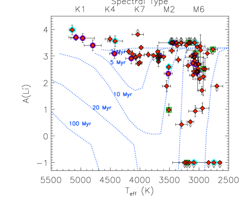
Figure 3: Lithium abundance versus effective temperature. The “lithium isochrones” by Baraffe et al. (2015) in the 2–100 Myr range are overlaid with dotted lines. Arrows refer to upper and lower limits. Open squares, circles, and pentagons represent the position of the class III, transitional disks, and sub-luminous or flat energy distribution targets, respectively. Spectral types as in Fig. 1 are also shown.

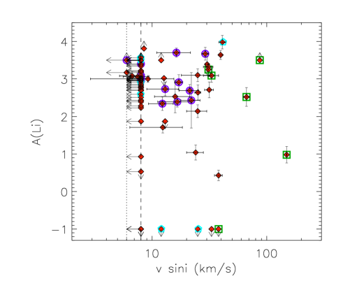
Figure 4: Lithium abundance versus projected rotational velocity. Symbols as in Fig. 3. The dashed and dotted lines represent the upper limits at 8 and 6 km/s of our VIS spectra acquired with the slit width at 0$\aas@@fstack{\prime\prime}$9 and 0$\aas@@fstack{\prime\prime}$4, respectively (see Frasca et al. 2017).

3.2 Spectral synthesis of Fe and Ba lines

The spectral synthesis for deriving iron and barium abundances was carried out by employing the code MOOG (Sneden 1973; 2013 version) and the Kurucz (1993) set of model atmospheres. We then adopted the stellar parameters ($T_{\rm eff}$, $\log g$, $v\sin i$) determined by Frasca et al. (2017) and considering the stars with: $i)$ $T_{\rm eff}>4400$ K, to avoid the contribution of molecular bands, which would severely affect the determination of [Fe/H] through their uncertain opacities (see, e.g., Appendix B in Biazzo et al. 2011a); $ii)$ low veiling ($r<1.0$), as it reduces the depth of absorption lines, introducing a further uncertainty in [Fe/H] determinations; $iii)$ low $v\sin i$ ($<40$ km/s) to avoid severe line blending. In the end, six targets fulfill these requirements (SSTc2d J160830.7-382827, RY Lup, MY Lup, Sz 68, Sz 133, and SSTc2d J160836.2-392302). SSTc2d J160830.7-382827 and MY Lup are weak accretors with transitional disks, RY Lup has a transitional disk, Sz 68 is a weak accretor, Sz 133 is a sub-luminous object, and SSTc2d J160836.2-392302 has a most probable transitional disk (see Ansdell et al. 2016; Alcalá et al. 2017 for details).

3.2.1 Iron abundance

Despite the extremely wide wavelength coverage, the relatively low resolution of the X-shooter spectra prevented us from using a very wide spectral range with unblended and isolated iron lines. For this reason, we chose to derive the iron abundance using the spectral synthesis method in a wavelength window of $\sim 20$ Å around the Li i line at 6707.8 Å. This spectral range proved to be very suitable for reliable iron abundance measurements (see D’Orazi et al. 2011, and references therein, for details). We considered the line list employed in D’Orazi et al. (2011), with carefully derived atomic parameters. As solar iron abundance we considered the value of Asplund et al. (2009), that is, $\log n({\rm Fe})_{\odot}=7.50\pm 0.04$ dex. We refer to D’Orazi et al. (2011), and references therein, for detailed explanations of the method.

For the six selected targets, we fixed within the MOOG code the appropriate spectral resolution, the limb-darkening coefficients (taken from Claret et al. 2012), the veiling $r_{6700}$, and the microturbulence $\xi=1.5$ km/s, which is typical of young stars similar to our targets (see, e.g., D’Orazi et al. 2011; Biazzo et al. 2011a, b). Then, we progressively changed the iron abundance until the best-fit (minimum of residuals) to the observed spectrum was obtained (see Fig. 5). As a by-product, the spectral synthesis around the Li line also allowed us to estimate the Li abundance, $A({\rm Li})^{\rm synth}$, for the six targets, that is found to be consistent within errors with the one obtained from the equivalent widths and the COGs (see Table 2 and Fig. 5). This allowed us to make an independent assessment of the lithium abundance for these stars.

The Fe abundance uncertainties are related both to the uncertainty in the best-fit model (we call this $\sigma_{1}$) and the errors in stellar parameters (which we call $\sigma_{2}$). Besides the uncertainty coming from the best-fit, $\sigma_{1}$ also includes errors in the continuum placement, that we estimated to be twice as large as the standard deviation obtained for the fit. We found that, at the average $T_{\rm eff}$ of 4800 K of our targets, $\sigma_{2}$ varies between 0.07 dex and 0.11 dex for typical uncertainties of $\pm$120 K and $\pm$0.2 dex in $T_{\rm eff}$ and $\log g$, respectively. Microturbulence velocity was fixed at 1.5 km/s, but typical errors of $\sim$0.2 km/s lead to a [Fe/H] uncertainty of $\pm 0.02$ dex. Other sources of error are the indetermination in $v\sin i$ and $r_{6700}$, which were fixed in our analysis. An uncertainty in $v\sin i$ of about 3 km/s may lead to errors of $\pm 0.06$ dex in iron abundance. The last source of uncertainty is veiling, that could be the largest for highly veiled spectra. However, for the low veiling values of the six targets here analyzed, an uncertainty of $\sim$0.1 in $r_{6700}$ translates into an error in [Fe/H] of $\pm 0.05$ dex. Final errors can be obtained by summing in quadrature the uncertainties from spectral synthesis and stellar parameters, plus additional contributions from rotational velocity and veiling. Typical uncertainties of $0.2-0.7$ dex for [Fe/H] are derived, depending on target. The major source of error is the best-fit procedure, mainly because of the uncertainties due to continuum placement.

Systematic (external) errors, caused for instance by the code and/or model atmosphere, should not strongly influence our abundance analysis, as widely discussed by D’Orazi et al. (2011).

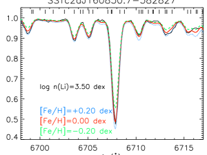
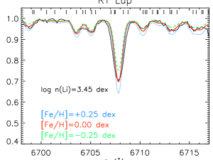
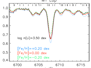
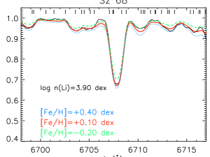
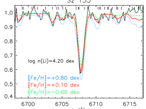
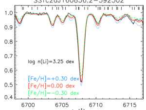
Figure 5: Observed spectrum (black line) and best-fit synthetic spectrum (red line) for the six targets analyzed for abundance measurements. The blue dashed and green dotted lines represent the [Fe/H] values due to uncertainties in the best-fit procedure (see text). Iron lines are indicated with short vertical lines in the upper part of each panel.

3.2.2 Barium abundance

We determined the abundance of the $s$-process element barium through spectral synthesis of the Ba ii line at $\lambda=5853.7$ Å. We checked for other Ba lines, such as the Ba ii lines at $\lambda$4554 Å, $\lambda$6141 Å, $\lambda$6496 Å, and the Ba i line at $\lambda$5535 Å, but all of them are affected by significant NLTE effects. Moreover, the second Ba ii line and the Ba i line are also strongly blended with iron lines (Mashonkina & Gehren 2000; Reddy & Lambert 2015; Korotin et al. 2015). We also tried to analyze other suitable lines of additional $s$-process elements (e.g., Y ii $\lambda\lambda$4398, 5087, 5200, 5205 Å, Ce ii $\lambda\lambda$4073, 4350, 4562 Å, Zr ii $\lambda\lambda$4161, 4209, 4443 Å, La ii $\lambda\lambda$4087, 4322, 4333 Å), but unfortunately with unsuccessful results, the reasons being: $i)$ the lines are too weak and/or blended with other nearby lines (due to the relatively low resolution of our data and the stellar rotation); $ii)$ most of those lines are in the UV-Blue (UVB) arm of the X-shooter spectrograph, where the continuum placement has a strong impact on the abundance estimate; $iii)$ the veiling contribution, even if low, and added to the aforementioned effects, makes the abundance measurement very uncertain. In addition, the $S/N$ ratio of the spectra is lower in the UVB arm than in the other spectrograph arms

Although the Ba line at $\lambda 5853.7$ Å does not experience severe hyperfine structure (hfs) and isotopic shifts, we decided to include them and employ those provided by McWilliam (1998) with the aim of obtaining the best possible result with the spectra at our disposal. We then adopted the isotopic solar mixtures by Anders & Grevesse (1989), that is, 2.42% for ¹³⁴Ba, 7.85% for ¹³⁶Ba, 71.94% for ¹³⁸Ba, 6.58% for ¹³⁵Ba, and 11.21% for ¹³⁷Ba. As expected, the results do not depend on the abundance ratio for even and odd isotopes. As for the iron abundance, we considered the solar barium abundance by Asplund et al. (2009), that is, $\log n({\rm Ba})_{\odot}=2.18\pm 0.09$ dex, and the stellar parameters by Frasca et al. (2017). Then, we ran MOOG fixing the spectral resolution, the limb-darkening coefficients (taken by Claret et al. 2012), the veiling $r_{5800}$ (assuming a mean value between $r_{5200}$ and $r_{6200}$; see Table 1), and the microturbulence $\xi=1.5$ km/s. The fitting procedure and the error estimates are the same as for the iron abundance determination described in the previous Section, and for the same six selected stars.

In Fig. 6 we show the spectral synthesis of the six targets in the wavelength region around the Ba ii line, with the corresponding error $\sigma_{1}$ (see Table 2). As done for the Fe abundance, to evaluate the impact of the variation of the stellar parameters ($T_{\rm eff}$, $\log g$, and $\xi$) and of $v\sin i$ and $r$, we varied each quantity separately (leaving the others unchanged) and checked the abundance sensitivity to that variation. A change of $\pm$120 K in $T_{\rm eff}$, $\pm$0.2 dex in $\log g$, and $\pm$0.2 km/s in $\xi$, leads to Ba abundance variations of 0.07 dex, 0.03 dex, and 0.15 dex, respectively. This means that the barium abundance measurement is strongly influenced by the microturbulence (also noted by other authors, for example, D’Orazi et al. 2012), as the barium line is close to the flat part of the curve of growth. Variations of 3 km/s in $v\sin i$ lead to 0.01 dex uncertainty in [Ba/H], while an uncertainty of about 0.1 in veiling yields an error of $\sim$0.15 dex in [Ba/H]. Therefore, veiling also has a strong influence on this element. We will discuss the impact of $\xi$ and $r_{5800}$ measurement on the determination of barium abundance in Sect. 4.4. The cumulative uncertainty in [Ba/H] can be obtained by summing in quadrature the uncertainties from the fit, those on the stellar parameters, and the additional contribution of the $v\sin i$ error (negligible) and veiling. The cumulative uncertainties in [Ba/H] measurements for our targets are of $\sim$0.2-0.7 dex, that is, they are dominated by the best-fit procedure.

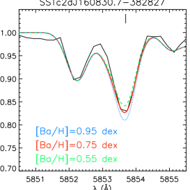
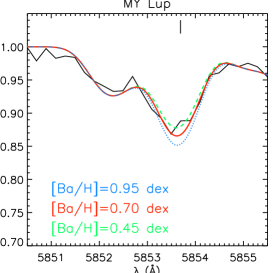
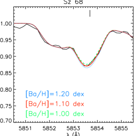
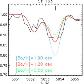
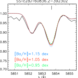
Figure 6: Visualization of spectral synthesis as in Fig. 5 but for the Ba ii line at $\lambda 5853.7$ Å. The barium line is marked with a short vertical line in the upper part of each panel.

Table 1: Stellar parameters. Object name, spectral type, effective temperature, surface gravity, rotational velocity, radial velocity, veiling at $\lambda$=5400 Å, $6200$ Å, and 7100 Å, measured and corrected lithium equivalent width and lithium abundance.

Name	SpT	$T_{\rm eff}$	$\log g$	$v\sin i$	$V_{\rm rad}$	$r_{5400}$	$r_{6200}$	$r_{7100}$	$EW_{\rm Li}$	$EW_{\rm Li}^{\rm corr}$	$A$(Li)
		(K)	(dex)	(km/s)	(km/s)				(mÅ)	(mÅ)	(dex)
Sample of class II YSOs by Alcalá et al. (2014)
Sz 66	M3	3351$\pm$ 47	3.81$\pm$0.21	$\leq$8.0	17.4$\pm$1.8	1.5	0.8	$\leq$0.2	370$\pm$10	481	2.86$\pm$0.12
AKC2006 19	M5	3027$\pm$ 34	4.45$\pm$0.11	$\leq$8.0	9.6$\pm$2.1	…	$\leq$0.2	$\leq$0.2	660$\pm$21	631	3.34$\pm$0.04
Sz 69	M4.5	3163$\pm$119	3.50$\pm$0.23	33.0$\pm$4.0	5.4$\pm$2.9	…	$\leq$0.2	$\leq$0.2	150$\pm$10	122	$<-1$
Sz 71	M1.5	3599$\pm$ 35	4.27$\pm$0.24	$\leq$8.0	11.7$\pm$1.9	0.6	0.5	0.3	540$\pm$12	720	3.00$\pm$0.16
Sz 72	M2	3550$\pm$ 70	4.18$\pm$0.28	$\leq$8.0	6.9$\pm$2.4	…	$\leq$0.2	$\leq$0.2	418$\pm$10	392	1.87$\pm$0.21
Sz 73	K7	3980$\pm$ 33	4.40$\pm$0.33	31.0$\pm$3.0	5.0$\pm$2.2	1.0	1.0	0.5	527$\pm$11	832	3.32$\pm$0.08
Sz 74	M3.5	3371$\pm$ 79	3.98$\pm$0.11	30.2$\pm$1.0	1.0$\pm$1.5	0.7	0.4	$\leq$0.2	472$\pm$12	535	3.39$\pm$0.20
Sz 83	K7	4037$\pm$ 96	3.5 $\pm$0.4	8.5$\pm$4.8	3.3$\pm$1.8	…	3.5	2.4	272$\pm$10	988	$>$3.81
Sz 84a	M5	3058$\pm$ 82	4.20$\pm$0.21	21.3$\pm$4.1	11.9$\pm$2.0	0.9	0.3	$\leq$0.2	490$\pm$12	531	2.69$\pm$0.16
Sz 130	M2	3448$\pm$ 62	4.48$\pm$0.10	$\leq$8.0	3.6$\pm$2.6	…	0.7	$\leq$0.2	455$\pm$10	579	$>$3.5
Sz88 A	M0	3700$\pm$ 19	3.77$\pm$0.47	$\leq$8.0	6.5$\pm$2.3	…	2.1	1.4	308$\pm$10	777	3.17$\pm$0.23
Sz88 B	M4.5	3075$\pm$111	4.08$\pm$0.12	$\leq$8.0	5.7$\pm$2.1	…	0.3	0.3	570$\pm$10	704	$>$3.50
Sz 91a	M1	3664$\pm$ 45	4.34$\pm$0.22	$\leq$8.0	19.0$\pm$2.4	0.9	0.6	0.4	480$\pm$10	681	3.00$\pm$0.22
Lup 713	M5.5	2943$\pm$109	3.89$\pm$0.13	24.0$\pm$4.0	3.9$\pm$3.3	…	…	$\leq$0.2	352$\pm$25	323	1.04$\pm$0.20
Lup 604s	M5.5	3014$\pm$ 62	3.89$\pm$0.12	31.5$\pm$2.8	2.7$\pm$1.9	…	$\leq$0.2	$\leq$0.2	575$\pm$25	546	2.71$\pm$0.21
Sz 97	M4	3185$\pm$ 78	4.14$\pm$0.16	25.1$\pm$1.5	2.4$\pm$2.2	0.7	$\leq$0.2	$\leq$0.2	525$\pm$15	497	2.64$\pm$0.20
Sz 99	M4	3297$\pm$ 98	3.89$\pm$0.21	38.0$\pm$3.0	3.2$\pm$3.1	…	$\leq$0.2	$\leq$0.2	213$\pm$15	186	0.43$\pm$0.14
Sz 100a	M5.5	3037$\pm$ 44	3.87$\pm$0.21	16.6$\pm$5.4	2.7$\pm$2.5	…	$\leq$0.2	$\leq$0.2	525$\pm$15	496	2.39$\pm$0.14
Sz 103	M4	3380$\pm$ 36	3.97$\pm$0.10	12.0$\pm$4.0	1.4$\pm$2.2	0.7	0.3	$\leq$0.2	517$\pm$15	564	$>$3.5
Sz 104	M5	3074$\pm$ 73	3.96$\pm$0.10	$\leq$8.0	2.3$\pm$2.3	…	$\leq$0.2	$\leq$0.2	570$\pm$24	542	2.83$\pm$0.24
Lup 706b	M7.5	2750$\pm$ 82	3.93$\pm$0.11	25.0$\pm$15.0	11.9$\pm$4.5	…	…	$\leq$0.2	$<$100d	$<$69	$<-1$
Sz 106b	M0.5	3691$\pm$ 35	4.82$\pm$0.13	$\leq$8.0	8.0$\pm$2.6	0.5	0.5	$\leq$0.2	515$\pm$12	612	$<$2.91
Par-Lup3-3	M4	3461$\pm$ 49	4.47$\pm$0.11	$\leq$8.0	3.5$\pm$2.5	…	$\leq$0.2	$\leq$0.2	560$\pm$25	534	3.20$\pm$0.11
Par-Lup3-4b	M4.5	3089$\pm$246	3.56$\pm$0.80	12.0$\pm$10.0	5.6$\pm$4.3	…	…	0.3	$<$100d	$<$93	$<-1$
Sz 110	M4	3215$\pm$162	4.31$\pm$0.21	$\leq$8.0	2.6$\pm$2.3	2.7	1.0	0.4	370$\pm$10	583	3.40$\pm$0.27
Sz 111a	M1	3683$\pm$ 34	4.66$\pm$0.21	$\leq$8.0	13.8$\pm$2.1	0.6	0.5	0.3	490$\pm$12	650	$<$2.95
Sz 112a	M5	3079$\pm$ 47	3.96$\pm$0.10	$\leq$8.0	6.2$\pm$1.7	…	$\leq$0.2	$\leq$0.2	590$\pm$12	562	3.03$\pm$0.12
Sz 113	M4.5	3064$\pm$114	3.76$\pm$0.27	$\leq$8.0	6.1$\pm$2.4	…	…	0.5	210$\pm$15	272	0.93$\pm$0.21
2MASS J16085953-3856275	M8.5	2649$\pm$ 31	3.98$\pm$0.10	$\leq$8.0	7.2$\pm$4.0	…	$\leq$0.2	$\leq$0.2	$<$80d	$<$48	$<-1$
SSTc2d 160901.4-392512	M4	3305$\pm$ 57	4.51$\pm$0.11	$\leq$8.0	15.9$\pm$0.7	0.7	$\leq$0.2	$\leq$0.2	565$\pm$20	538	$>$3.5
Sz 114	M4.8	3134$\pm$ 35	3.92$\pm$0.12	$\leq$8.0	4.0$\pm$2.4	0.6	0.3	0.3	565$\pm$10	698	$>$3.5
Sz 115	M4.5	3124$\pm$ 42	3.90$\pm$0.21	9.2$\pm$6.3	6.4$\pm$2.3	…	$\leq$0.2	$\leq$0.2	579$\pm$15	551	0.93$\pm$0.21
Lup 818s	M6	2953$\pm$ 59	3.97$\pm$0.11	12.4$\pm$6.0	5.1$\pm$2.0	…	$\leq$0.2	$\leq$0.2	459$\pm$2	430	1.71$\pm$0.15
Sz 123 Aa	M1	3521$\pm$ 70	4.46$\pm$0.13	12.3$\pm$3.0	16.8$\pm$1.8	1.2	0.6	$\leq$0.2	410$\pm$12	499	2.34$\pm$0.18
Sz 123 Bb	M2	3513$\pm$ 45	4.17$\pm$0.22	$\leq$8.0	7.4$\pm$2.3	0.8	0.6	$\leq$0.2	421$\pm$8	513	2.59$\pm$0.11
SST-Lup3-1	M5	3042$\pm$ 43	3.95$\pm$0.11	$\leq$8.0	6.3$\pm$2.6	…	$\leq$0.2	$\leq$0.2	530$\pm$15	501	2.43$\pm$0.14
Sample of class II YSOs by Alcalá et al. (2017)
Sz 65	K7	4005$\pm$ 75	3.85$\pm$0.26	$\leq$8.0	$-$2.7$\pm$2.0	0.3	0.3	$\leq$0.2	602$\pm$10	667	3.03$\pm$0.13
AKC2006 18	M6.5	2930$\pm$ 45	4.46$\pm$0.11	$\leq$8.0	9.1$\pm$2.3	…	$\leq$0.2	$\leq$0.2	545$\pm$100	515	2.23$\pm$0.72
SSTc2d J154508.9-341734	M5.5	3242$\pm$205	3.33$\pm$0.77	$\leq$8.0	$-$0.8$\pm$2.7	…	0.8	0.7	$<$60d	$<$57	$<-1$
Sz 68	K2	4506$\pm$ 82	3.68$\pm$0.12	39.6$\pm$1.2	$-$4.3$\pm$1.8	0.3	0.3	0.4	441$\pm$10	571	3.64$\pm$0.12
SSTc2d J154518.5-342125	M6.5	2700$\pm$100	3.45$\pm$0.11	13.0$\pm$6.0	4.4$\pm$2.9	…	$\leq$0.2	$\leq$0.2	525$\pm$15	493	$<$1.87
Sz81 A	M4.5	3077$\pm$151	3.48$\pm$0.11	$\leq$8.0	$-$0.1$\pm$2.9	…	0.3	$\leq$0.2	510$\pm$20	554	2.96$\pm$0.25
Sz81 B	M5.5	2991$\pm$ 76	3.53$\pm$0.11	25.0$\pm$5.0	1.2$\pm$2.4	…	0.3	$\leq$0.2	445$\pm$15	478	2.14$\pm$0.17
Sz 129	K7	4005$\pm$ 45	4.49$\pm$0.25	$\leq$10.0	3.2$\pm$2.5	1.4	1.0	$\leq$0.2	440$\pm$11	627	2.76$\pm$0.05
SSTc2d J155925.2-423507	M5	2984$\pm$ 82	4.41$\pm$0.12	$\leq$8.0	6.5$\pm$2.5	…	$\leq$0.2	$\leq$0.2	660$\pm$40	631	3.37$\pm$0.05
RY Lupa	K2	5082$\pm$118	3.87$\pm$0.22	16.3$\pm$5.3	1.3$\pm$2.0	0.4	0.5	$\leq$0.2	377$\pm$10	455	3.70$\pm$0.12
SSTc2d J160000.6-422158	M4.5	3086$\pm$ 82	4.03$\pm$0.11	$\leq$8.0	2.5$\pm$2.2	…	$\leq$0.2	$\leq$0.2	580$\pm$20	552	2.96$\pm$0.15
SSTc2d J160002.4-422216	M4	3159$\pm$140	4.00$\pm$0.48	$\leq$8.0	2.6$\pm$2.6	0.3	$\leq$0.2	$\leq$0.2	660$\pm$80	632	$>$3.5
SSTc2d J160026.1-415356	M5.5	2976$\pm$221	3.97$\pm$0.35	$\leq$8.0	$-$1.1$\pm$2.3	…	0.3	$\leq$0.2	560$\pm$50	610	3.22$\pm$0.58
MY Lupa	K0	4968$\pm$200	3.72$\pm$0.18	29.1$\pm$2.0	4.4$\pm$2.1	$\leq$0.2	$\leq$0.2	$\leq$0.2	468$\pm$10	454	3.67$\pm$0.17
Sz 131	M3	3300$\pm$122	4.29$\pm$0.36	$\leq$8.0	2.4$\pm$2.2	…	0.3	$\leq$0.2	535$\pm$30	584	$>$3.5
Sz 133b	K5	4420$\pm$129	3.96$\pm$0.51	$\leq$8.0	0.7$\pm$2.5	0.7	0.7	0.5	420$\pm$25	643	3.56$\pm$0.20
SSTc2d J160703.9-391112b	M4.5	3072$\pm$ 55	4.01$\pm$0.11	$\leq$8.0	1.8$\pm$2.7	…	$\leq$0.2	$\leq$0.2	680$\pm$50	652	$>$3.50
SSTc2d J160708.6-391408c	…	3474$\pm$206	4.18$\pm$0.56	$\leq$8.0	$-$4.2$\pm$2.9	…	1.0	0.9	504$\pm$65	932	$>$3.50
Sz 90	K7	4022$\pm$ 52	4.24$\pm$0.42	$\leq$8.0	1.6$\pm$2.3	0.5	0.5	$\leq$0.2	491$\pm$10	587	2.71$\pm$0.08
Sz 95	M3	3443$\pm$ 53	4.37$\pm$0.12	$\leq$8.0	$-$2.8$\pm$2.3	…	$\leq$0.2	$\leq$0.2	585$\pm$10	559	3.49$\pm$0.02
Sz 96	M1	3702$\pm$ 57	4.50$\pm$0.23	$\leq$8.0	$-$2.7$\pm$2.6	0.3	0.4	$\leq$0.2	595$\pm$10	683	2.99$\pm$0.13
2MASS J16081497-3857145a	M5.5	3024$\pm$ 46	3.96$\pm$0.23	22.0$\pm$4.2	6.0$\pm$2.9	…	$\leq$0.2	$\leq$0.2	525$\pm$100	496	2.43$\pm$0.74
Sz 98	K7	4080$\pm$ 71	4.10$\pm$0.23	$\leq$8.0	$-$1.4$\pm$2.1	0.5	0.6	$\leq$0.2	508$\pm$10	633	2.97$\pm$0.11
Lup 607	M6.5	3084$\pm$ 46	4.48$\pm$0.11	$\leq$8.0	6.8$\pm$2.4	…	$\leq$0.2	$\leq$0.2	539$\pm$20	511	2.43$\pm$0.11
Sz 102b	K2	5145$\pm$ 50	4.10$\pm$0.50	41.0$\pm$2.8	21.6$\pm$12.4	…	2.5	2.0	196$\pm$50	595	3.98$\pm$0.18
SSTc2d J160830.7-382827	K2	4797$\pm$145	4.09$\pm$0.23	$\leq$8.0	1.2$\pm$1.9	0.1	$\leq$0.2	$\leq$0.2	436$\pm$10	421	3.40$\pm$0.20
SSTc2d J160836.2-392302a	K6	4429$\pm$ 83	4.04$\pm$0.13	$\leq$8.0	2.2$\pm$2.1	0.3	0.3	$\leq$0.2	454$\pm$35	501	3.09$\pm$0.18
Sz 108 B	M5	3102$\pm$ 59	3.86$\pm$0.22	$\leq$8.0	0.2$\pm$2.2	…	$\leq$0.2	$\leq$0.2	495$\pm$25	467	2.28$\pm$0.16
2MASS J16085324-3914401	M3	3393$\pm$ 85	4.24$\pm$0.41	$\leq$8.0	0.9$\pm$2.2	…	0.3	$\leq$0.2	577$\pm$12	663	3.50$\pm$0.03
2MASS J16085373-3914367	M5.5	2840$\pm$200	3.60$\pm$0.45	$\leq$8.0	6.1$\pm$6.9	…	$\leq$0.2	$\leq$0.2	$<$100d	$<$70	$<-1$
2MASS J16085529-3848481	M4.5	2899$\pm$ 55	3.99$\pm$0.11	$\leq$8.0	$-$1.1$\pm$2.4	…	$\leq$0.2	$\leq$0.2	591$\pm$40	561	2.51$\pm$0.41
SSTc2d J160927.0-383628a	M4.5	3147$\pm$ 58	4.00$\pm$0.10	$\leq$8.0	3.4$\pm$2.2	…	1.5	0.5	132$\pm$15	209	$<$0.53
Sz 117	M3.5	3470$\pm$ 51	4.10$\pm$0.32	$\leq$8.0	$-$1.4$\pm$2.2	0.7	0.4	$\leq$0.2	569$\pm$15	651	$>$3.5
Sz 118	K5	4067$\pm$ 82	4.47$\pm$0.37	$\leq$8.0	$-$0.8$\pm$2.3	0.5	0.5	$\leq$0.2	558$\pm$10	671	2.95$\pm$0.13
2MASS J16100133-3906449	M6.5	3018$\pm$ 72	3.77$\pm$0.23	15.9$\pm$5.4	0.1$\pm$2.6	…	$\leq$0.2	$\leq$0.2	550$\pm$50	521	2.53$\pm$0.43
SSTc2d J161018.6-383613	M5	3012$\pm$ 48	3.98$\pm$0.10	$\leq$8.0	$-$0.2$\pm$2.5	…	$\leq$0.2	$\leq$0.2	570$\pm$15	541	2.69$\pm$0.15
SSTc2d J161019.8-383607	M6.5	2861$\pm$ 69	4.00$\pm$0.10	25.0$\pm$7.0	1.8$\pm$2.5	…	$\leq$0.2	$\leq$0.2	660$\pm$50	630	3.10$\pm$0.17
SSTc2d J161029.6-392215a	M4.5	3098$\pm$ 59	4.02$\pm$0.10	13.0$\pm$4.0	$-$2.7$\pm$2.2	…	$\leq$0.2	$\leq$0.2	550$\pm$20	522	2.73$\pm$0.18
SSTc2d J161243.8-381503	M1	3687$\pm$ 22	4.57$\pm$0.21	$\leq$8.0	$-$2.3$\pm$2.4	…	0.3	$\leq$0.2	534$\pm$10	585	2.79$\pm$0.19
SSTc2d J161344.1-373646	M5	3028$\pm$ 78	4.25$\pm$0.14	$\leq$8.0	$-$1.2$\pm$2.3	…	0.5	0.3	388$\pm$15	503	2.39$\pm$0.13

Table 1: Continued.

Name	SpT	$T_{\rm eff}$	$\log g$	$v\sin i$	$V_{\rm rad}$	$r_{5400}$	$r_{6200}$	$r_{7100}$	$EW_{\rm Li}$	$EW_{\rm Li}^{\rm corr}$	$A$(Li)
		(K)	(dex)	(km/s)	(km/s)				(mÅ)	(mÅ)	(dex)
Sample of class II YSOs from the ESO Archive
GQ Lup	K6	4192$\pm$ 65	4.12$\pm$0.36	$\leq$6.0	4.9$\pm$1.3	0.8	0.5	0.3	483$\pm$10	647	3.17$\pm$0.10
Sz 76a	M4	3440$\pm$ 60	4.41$\pm$0.26	$\leq$6.0	1.4$\pm$1.0	0.7	$\leq$0.2	$\leq$0.2	609$\pm$50	583	$>$3.5
Sz 77	K7	4131$\pm$ 48	4.28$\pm$0.31	6.7$\pm$1.5	2.4$\pm$1.5	0.5	0.4	$\leq$0.2	573$\pm$15	663	3.08$\pm$0.12
RX J1556.1-3655	M1	3770$\pm$ 70	4.75$\pm$0.21	12.7$\pm$1.3	2.6$\pm$1.2	…	1.4	0.3	388$\pm$20	671	$<$3.02
IM Lupa	K5	4146$\pm$ 95	3.80$\pm$0.37	17.1$\pm$1.4	$-$0.5$\pm$1.3	$\leq$0.2	$\leq$0.2	$\leq$0.2	566$\pm$10	545	2.91$\pm$0.20
EX Lup	M0	3859$\pm$ 62	4.31$\pm$0.29	7.5$\pm$1.9	1.9$\pm$1.4	1.0	0.7	$\leq$0.2	500$\pm$15	642	3.06$\pm$0.10
Sample of class III YSOs by Frasca et al. (2017) observed within the GTO by Alcalá et al. (2011)
Sz 94	M4	3205$\pm$ 59	4.21$\pm$0.24	38.0$\pm$3.0	7.8$\pm$2.0	…	$\leq$0.2	$\leq$0.2	$<$28e	$<$1	$<-1$
Par-Lup3-1	M6.5	2766$\pm$ 77	3.48$\pm$0.11	31.0$\pm$7.0	4.9$\pm$3.9	…	$\leq$0.2	$\leq$0.2	685$\pm$80	654	$<$3.25
Par-Lup3-2	M5	3060$\pm$ 61	3.91$\pm$0.24	33.0$\pm$5.0	5.0$\pm$2.5	…	$\leq$0.2	$\leq$0.2	602$\pm$35	574	3.09$\pm$0.18
Sz 107	M5.5	2928$\pm$100	3.52$\pm$0.13	66.6$\pm$4.1	6.1$\pm$3.8	…	$\leq$0.2	$\leq$0.2	570$\pm$30	540	2.52$\pm$0.25
Sz 108 A	…	3676$\pm$ 34	4.50$\pm$0.21	$\leq$8.0	0.4$\pm$2.2	0.5	0.4	$\leq$0.2	628$\pm$10	723	3.02$\pm$0.04
Sz 121	M4	3178$\pm$ 61	4.08$\pm$0.12	87.0$\pm$8.0	14.1$\pm$4.4	…	$\leq$0.2	$\leq$0.2	635$\pm$25	607	$>$3.50
Sz 122	M2	3511$\pm$ 27	4.58$\pm$0.21	149.2$\pm$1.0	17.9$\pm$3.0	…	$\leq$0.2	$\leq$0.2	300$\pm$25	274	0.98$\pm$0.22

^a YSO with transitional disk; ^b Sub-luminous YSO; ^c Flat source (see Alcalá et al. 2017); ^d Lithium non detected because of low $S/N$; ^e star with no lithium (see text for details).
Notes: Spectral types for class II and III YSOs were taken from Alcalá et al. (2017) and Manara et al. (2013), respectively, while effective temperatures, surface gravities, projected rotational velocities, radial velocities, and veiling in three spectral regions from Frasca et al. (2017).

Table 2: Iron, barium, and lithium abundances measured through spectral synthesis. Errors refer to the best-fit procedure ($\sigma_{1}$), the main source of uncertainty (see text for details).

Name	[Fe/H]	[Ba/H]	$A({\rm Li})^{\rm synth}$
	(dex)	(dex)	(dex)
SSTc2d J160830.7-382827	$0.00\pm 0.20$	$0.75\pm 0.20$	$3.50\pm 0.15$
RY Lup	$0.00\pm 0.25$	$1.10\pm 0.30$	$3.45\pm 0.20$
MY Lup	$0.00\pm 0.20$	$0.70\pm 0.25$	$3.50\pm 0.15$
Sz 68	$0.10\pm 0.30$	$1.10\pm 0.10$	$3.90\pm 0.20$
Sz 133	$0.10\pm 0.70$	$1.20\pm 0.70$	$4.00\pm 0.20$
SSTc2d J160836.2-392302	$0.00\pm 0.30$	$1.05\pm 0.10$	$3.25\pm 0.15$

4 Results and discussion

4.1 Lithium abundance, comparison with models, and implications

Our sample comprises stars with $M_{\star}\sim 0.025-1.8M_{\odot}$ (see Alcalá et al. 2017; Frasca et al. 2017). Considering the sub-sample of stars with masses $>0.5M_{\odot}$, we do not find an indication of Li depletion, $\sim 3.3$ dex being the mean abundance of these stars. The situation is different for the sub-sample of stars with masses in the range $0.2-0.5M_{\odot}$ (Fig. 7). For these stars we can apply the so-called lithium test, as first proposed by Palla et al. (2005) for targets in Orion. Briefly, this is a useful clock based on the possibility that stars deplete their initial lithium content during the early phases of PMS contraction. It has been demonstrated that the theoretical assumptions required to study Li depletion history have little uncertainty, as for fully convective stars the depletion mostly depends on $T_{\rm eff}$ (Bildsten et al. 1997). At the same time, models show that stars with mass in the range $\sim 0.5-0.2M_{\odot}$ start to deplete Li after 4–15 Myr and completely destroy it after a further 10–15 Myr (e.g., Baraffe et al. 2015, and references therein). We therefore can compare the nuclear ages derived from the lithium test with the isochronal ages derived from the Hertzsprung-Russell (HR) diagram. First evidence of a Li depletion boundary for PMS stars have been reported by Song et al. (2002) and White & Hillenbrand (2005), where the timescale of Li depletion turned out to be larger than the isochronal age.

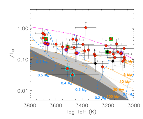
Figure 7: Hertzsprung-Russell diagram for the sample stars with masses $\sim\leavevmode\nobreak\ 0.2-0.5\leavevmode\nobreak\ M_{\odot}$. The shaded regions indicate different levels of predicted Li depletion: up to a factor of 10 (light gray) and more (dark gray) below the initial value and according to the models of Baraffe et al. (2015). Masses from evolutionary tracks and isochronal ages are labeled. Black diamonds refer to targets showing depletion (i.e., Sz 99, Sz 69, and Sz 94; see text and Fig. 8). Open squares, circles, and pentagons represent the position of the class III, transitional disk, and sub-luminous or flat targets, respectively.

In order to investigate the lithium depletion in our sample, we applied the procedure already tested in some sub-groups of the Orion SFR (see Palla et al. 2005, 2007; Sacco et al. 2007) for objects with mass in the range $0.2<M_{\star}<0.5M_{\odot}$. The derived lithium abundances are displayed in Fig. 8 versus the age derived by Frasca et al. (2017) using the Baraffe et al. (2015) isochrones. The figure shows a trend for the youngest stars to preserve their initial lithium content. Excluding the stars with upper and lower limits, the mean $A$(Li) for the sub-sample is around 2.74 dex with a standard deviation of 0.72 dex. Therefore, we consider as probable Li depleted targets those lying below a threshold of $\sim$2 dex in lithium abundance.

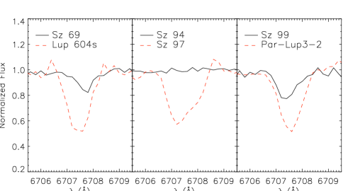
Figure 9: Portions of spectra for the three Li depleted stars (solid lines) around the lithium line at $\lambda=6707.8$ Å. Dashed lines represent the spectra of three non-Li depleted stars with similar stellar parameters (i.e., $T_{\rm eff}$, $\log g$, $v\sin i$, and $r_{6700}$).

Considering the stars with isochronal ages $>2$ Myr, five class II objects (SSTc2dJ160927.0-383628, Sz 69, SSTc2dJ154508.9-341734, Sz 72, and Sz 99) and one class III (Sz 122) appear below the threshold we defined, while two other class II YSOs (Sz 108B and Sz 123A) are close to it. However, slightly higher values of veiling, still within the uncertainty of $\sim 0.1-0.2$, could influence their abundance determination, placing them close to the non-depleted YSOs. Among the six apparently depleted targets, Sz 72 has an effective temperature of 3550 K, that is, in the $T_{\rm eff}$ within the range of overlap between the two curves of growth used to derive abundance (see Sect. 3.1.2), hence its $A$(Li) is rather uncertain. Then, for SSTc2d J160927.0-383628 and SSTc2d J154508.9-341734 a veiling of $r_{6700}\sim 1$ is measured, hence their lithium abundances may be strongly influenced by strong continuum excess emission, while the class III star Sz 122 could be a spectroscopic binary, as stressed in Sect. 3.1.2. In summary, among the six YSOs below our lithium depletion threshold, there are only two cases in which lithium depletion can be clearly assessed; these are Sz 99 and Sz 69. We thus consider these two YSOs as the most probable lithium depleted targets in our sample. In addition, we also include Sz 94, a class III object for which lithium has not been detected either by us or other authors (Mortier et al. 2011; Manara et al. 2013; Stelzer et al. 2013), but its radial velocity and the proper motion reported by López Martí et al. (2011) are consistent with the Lupus SFR. The profile of the Li i $\lambda$6707.8 Å line for these three YSOs is shown in Fig. 9 together with the spectra of three targets with similar stellar parameters. The figure clearly shows the much weaker (or absent) lithium line for the three most probable Li-depleted stars, when compared with undepleted YSOs of similar $T_{\rm eff}$, $\log g$, $v\sin i$, and veiling.

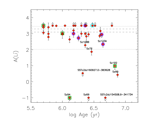
Figure 8: Li abundance versus age for stars with mass in the range $0.2-0.5M_{\odot}$. Symbols are the same as in Fig. 3. The dashed horizontal lines mark the region of the interstellar lithium abundance (3.1–3.3 dex). Dotted lines represent $\pm 1\sigma$ from the mean lithium abundance of this sub-sample. The labeled stars are those discussed in the text.

The existence of very young Li-poor low-mass stars in Lupus allowed us to perform a comparison between theoretical and analytical models of early nuclear burning. We therefore adopted the stellar masses and isochronal ages determined by Frasca et al. (2017) based on the PMS models of Baraffe et al. (2015), and applied the procedure described in Palla et al. (2005). Errors on both quantities were estimated from the uncertainties on luminosity and effective temperature provided by Alcalá et al. (2017) and Frasca et al. (2017), respectively. As stressed by Frasca et al. (2017), individual ages can be affected by uncertainties depending on the data errors and the adopted set of evolutionary tracks. As such, these ages must be taken with care. We can compare these results with the analytic estimates derived by Bildsten et al. (1997) for fully convective stars undergoing gravitational contraction at nearly constant $T_{\rm eff}$, assuming fast and complete mixing, and with negligible influence of degeneracy during the depletion, that is, in the mass range $0.2M_{\odot}\raisebox{-2.15277pt}{$\>\stackrel{{\scriptstyle\textstyle<}}{{\sim}}\>$}M_{\star}\raisebox{-2.15277pt}{$\>\stackrel{{\scriptstyle\textstyle<}}{{\sim}}\>$}0.5M_{\odot}$. Bildsten et al. (1997) derived relations for the time variation of the luminosity (see their Eq. 4) and of the amount of Li depletion (see their Eq. 11). Taking into account the measured luminosity and effective temperature, we can apply those equations and obtain a mass-depletion time plot. The results for the three Li-depleted stars are shown in Fig. 10. The line with positive slope represents the mass-age relation for each star at given $T_{\rm eff}$ and $L_{\star}$. The line with negative slope is the mass-age relation for a fixed Li abundance equal to that measured in each target. The intersection of these two lines yields the combination of mass and age at given $T_{\rm eff}$, luminosity, and lithium depletion. The derived values of nuclear masses and ages ($M_{\rm Li}$, $t_{\rm Li}$), together with those obtained by Frasca et al. (2017) through HR diagram ($M_{\rm HRD}$, $t_{\rm HRD}$) for the three stars, are listed in Table 3. The three stars are within the bounded region predicted by the Bildsten et al. (1997) analysis, but both masses and ages from Baraffe et al. (2015) models are discrepant when compared to the nuclear masses and ages. In fact, while the HR diagram indicates masses of $\sim 0.2-0.3$ $M_{\odot}$ and ages of $\sim 1-7$ Myr, the amount of lithium depletion can only be explained by more massive ($\sim 0.5$ $M_{\odot}$) and older ($\sim 15$ Myr) stars (see Fig. 10). In all cases, the derived values of lithium abundance yield ages that are inconsistent with the isochronal ones: these targets have experienced too much burning for the estimated isochronal ages. In order to reconcile the two estimates, the stellar luminosity should be decreased by a factor of $\sim 2-5$ and/or the effective temperature increased by several hundreds of Kelvin (see Fig. 7), which is several times more than the errors in these quantities. As pointed out by several authors (see Hartmann 2003; Palla et al. 2007, and references therein), the discrepancies may be explained as being due to a combination of effects, such as poorly known stellar (e.g., binarity, photometric variability, atmospheric parameters) and cluster (e.g., distance, extinction) properties. At the same time, an increase of the Li abundance up to the interstellar value would require an initial equivalent width a factor of $\sim 3-10$ larger than measured, which seems inconsistent if we take into account the uncertainties estimated in Section 3.1.2. Moreover, the influence of veiling in the $EW_{\rm Li}$ measurements is excluded because the three targets show $r_{6700}$ close to zero. In particular, to obtain $A$(Li)$\sim 3$ these targets should have a veiling of at least $\sim$3, which is not possible given their low level of continuum excess emission (see Alcalá et al. 2014, 2017).

We also compared our results with recent self-consistent calculations coupling numerical hydrodynamics simulations of collapsing pre-stellar cores and stellar evolution models of accreting objects (Baraffe et al. 2017). These models predict that early accretion of material with low internal energy (‘cold accretion’) or early accretion of material with energy depending on the accretion rate (‘hybrid accretion’) can produce objects with abnormal Li depletion, at odds with predictions from non-accreting stellar evolution models (Baraffe et al. 2017, and references therein). In particular, accretion bursts with typical accretion rates $\dot{M}_{\rm burst}>10^{-4}M_{\odot}$ yr^-1 may gravitationally compress the star, increasing its core temperature and pressure and triggering the early onset of lithium burning within a few Myr. Efficient large-scale convection, such as in low-mass PMS stars, would then rapidly deplete lithium throughout the star. Figure 11 shows the surface lithium abundances as a function of effective temperature in accreting models by Baraffe et al. (2017) under cold and hybrid accretion scenarios for ages at 2, 5, 10, and 20 Myr (the median age of our data was estimated to be $\sim 2$ Myr; Frasca et al. 2017). Our Li depleted targets show a content of lithium which is not reproduced by early accretion models. The latter predict less lithium depletion at the ages and masses (effective temperatures) of our targets. Only for one source do the models seem to reproduce the observed lithium abundance but for an age ($\sim 20$ Myr) inconsistent with the Lupus clouds. We conclude that early accretion models are not able to reproduce the lithium depletion of such a rare object (3/89, i.e. $\sim 3\%$).

Therefore, we are not able to draw final conclusions about the origin of the lithium depletion in the three targets. We support the recent suggestion by Baraffe et al. (2017) to devote more observational effort to characterize objects with abnormal Li depletion in young clusters, normally considered as outliers and often rejected from analyses.

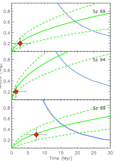
Figure 10: Mass versus age for the three stars with evidence of Li depletion. The curves at a given luminosity (solid green line with positive slope) and at a given lithium abundance (solid blue line with negative slope) were computed for the values of $T_{\rm eff}$, luminosity, and lithium depletion given in Table 3. The dashed and dotted curves represent the uncertainty ranges in the observed luminosity and in the measured abundance, respectively. They define the locus where the values of mass and time are consistent with the observations. For Sz 69 and Sz 94 no errors in Li abundances are reported because their values, consistent with zero, are upper limits. The diamonds give the mass and age from theoretical PMS tracks and isochrones, with typical errors of $\sim 0.1$ $M_{\odot}$ and $\sim 3$ Myr, respectively (see Frasca et al. 2017).

Table 3: Lithium depleted stars and their properties.

Name	$L_{\star}$	$T_{\rm eff}$	$A$(Li)	$M_{\rm HRD}$	$t_{\rm HRD}$	$M_{\rm Li}$	$t_{\rm Li}$
	($L_{\odot}$)	(K)	(dex)	($M_{\odot}$)	(Myr)	($M_{\odot}$)	(Myr)
Sz 69	$0.088\pm 0.041$	$3163\pm 119$	$<-1$	$0.2$	$2.6$	$\sim 0.6$	$\sim 19$
Sz 94	$0.174\pm 0.061$	$3205\pm 59$	$<-1$	$0.2$	$1.3$	$\sim 0.9$	$\sim 14$
Sz 99	$0.074\pm 0.034$	$3297\pm 98$	$0.43\pm 0.14$	$0.3$	$7.5$	$\sim 0.5$	$\sim 16$

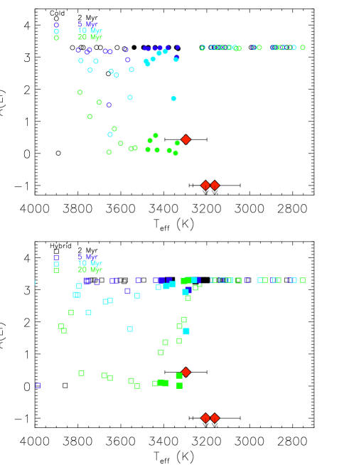
Figure 11: Surface lithium abundance as a function of effective temperature in accreting models under the cold (upper panel) and hybrid (bottom panel) accretion scenarios computed by Baraffe et al. (2017). Black, blue, light blue, and green symbols refer to predictions computed at 2, 5, 10, and 20 Myr, respectively. Filled symbols refer to models that predict a final stellar mass close to that of our Li depleted targets (i.e., $\sim 0.2-0.3M_{\odot}$). The positions of three Li depleted targets are shown with big red diamonds.

4.2 Iron abundance and comparison with previous works

Only one of our targets (namely, RY Lup) is in common with previous studies of iron abundance in the literature. For this star, we obtain a best-fit at [Fe/H]=$0.00\pm 0.25$, which is in agreement with the value of [Fe/H]=$-0.09\pm 0.13$ derived by Padgett (1996).

In Fig. 12 the distribution of our [Fe/H] measurements in Lupus is compared with the previous estimates by Padgett (1996) and Santos et al. (2008). In the first case, only the abundance of RY Lup was measured. In the second work, the average value obtained by analyzing four class III stars was ¡[Fe/H]¿=$-0.05\pm 0.01$, which is in agreement with our estimate. We note that, even if our measurements have larger uncertainties when compared with previous works (mainly because of the relatively low spectral resolution of the instrument used here), our distribution is narrow, peaked at $\sim 0.00$ dex with a standard deviation of 0.05 dex.

We stress that our abundance determination on class II targets is one of the few in which the contribution of veiling has been taken into account. A previous paper providing abundance determination for “deveiled” class II targets is that by D’Orazi et al. (2011) focused on the Taurus-Auriga SFR, where the authors find that class II and class III objects share the same chemical composition, indicating that the presence of a circumstellar accretion disk does not affect the stellar photospheric abundances. Other older analyses in class II targets did not consider the correction for the veiling, claiming that the derived iron abundance had to be treated as a lower limit (see, e.g., Padgett 1996).

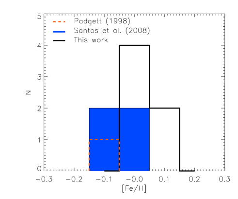
Figure 12: Comparison of our [Fe/H] with previous estimates by Padgett (1996) and Santos et al. (2008).

4.3 Iron abundance in the context of young stellar clusters

Recent works have shown that nearby ($<500$ pc) young open clusters span a range in [Fe/H] from $\sim-0.20$ to $\sim+0.30$ dex, but the youngest associations ($\raisebox{-2.15277pt}{$\>\stackrel{{\scriptstyle\textstyle<}}{{\sim}}\>$}100$ Myr) are generally clustered around the low metallicity values (see Fig. 13 in Biazzo et al. 2011a and Fig. 10 in Spina et al. 2014b). Because of their young ages, these regions did not have time to migrate through the Galactic disk. Therefore, their metal content should be representative of the present chemical pattern of the nearby interstellar gas from which their members formed, with negligible effects of chemical evolution (Biazzo et al. 2011a, and references therein). Spina et al. (2014b) concluded that since the chemical content provides a powerful tool for tagging groups of stars to a common formation site, these different young regions should share the same origin. They also report the metallicity distribution of regions younger than 100 Myr, separating clusters associated and not associated with the Gould Belt (see their Fig. 11), a disk-like structure made up of gas, young stars, and associations, whose origin remains somewhat controversial (see, e.g., Guillout et al. 1998; Bally 2008, and references therein). Spina et al. (2014b) also claim that star-forming regions and young open clusters associated with the Gould Belt show a metallicity lower than the solar value, and this could be the reason for the “non metal-rich” nature of the youngest stars in the solar vicinity.

Our determination of iron abundance for the Lupus targets with the X-shooter spectrograph is not as accurate as in the cited works, mainly because of the relatively low resolution of our spectra, but, within the errors, it is in line with recent results. However, we caution about the conclusion related to the Gould Belt for a number of reasons: the number statistics of the YSOs in the regions studied so far is still too low, the abundance determinations are rather heterogeneous because of the different methodologies used to derive them, and the uncertainties in the distance and proper motion of the studied YSOs are still rather high. Therefore, additional accurate and homogeneous determinations of elemental abundance and kinematics are needed to further investigate this issue. Present and future facilities both from space (e.g., Gaia) and from the Earth (e.g., the Gaia-ESO Survey) will allow us to trace dynamically and chemically our Galactic disk with unprecedented accuracy.

4.4 The barium problem

In Fig. 13 we show the [Ba/Fe] ratio versus mean age for targets in clusters studied by several authors (D’Orazi et al. 2009, 2012; De Silva et al. 2013; Reddy & Lambert 2015). For homogeneity reasons, we considered only dwarf targets analyzed with similar methods to ours. The Ba abundance shows an increasing trend with decreasing age, as already reported in previous works (e.g., D’Orazi et al. 2009; De Silva et al. 2013; Yong et al. 2012; Jacobson & Friel 2013). To our knowledge, the sample of dwarfs in Lupus is the youngest one analyzed so far for barium abundance determinations.

For targets older than $\sim$500 Myr, the trend of increasing [Ba/Fe] with decreasing cluster age was interpreted by D’Orazi et al. (2009) as an indication that low-mass ($<$ $1.5\,M_{\odot}$) AGB stars contributed more importantly to the chemical evolution of the Galactic disk than previously assumed by models (see Fig. 13). Applying $s$-process yields in which the neutron source was larger by a factor six than in previous models, D’Orazi et al. (2009) could reproduce the observed trend (see also Maiorca et al. 2014). On the other hand, as the same authors acknowledge, it would be difficult to imagine a process capable of creating barium in the last 500 Myr of Galactic evolution, unless local enrichment is assumed. Thus, in agreement with other works analyzing dwarf stars in 30-50 Myr old associations and clusters (e.g., D’Orazi et al. 2009, 2012, 2017), we are still facing a barium conundrum. In our case, the behavior is even more extreme, because for the Lupus SFR our [Ba/Fe] values are $\raisebox{-2.15277pt}{$\>\stackrel{{\scriptstyle\textstyle>}}{{\sim}}\>$}0.7$ dex (Fig. 13). If, on one side, the sharp function with age is evident, on the other, whether this corresponds to a real increase in the Ba abundance or whether it depends on the methodologies used to derive the abundance is still a matter of debate (see also D’Orazi et al. 2017). To spot possible artifacts in our analysis of Ba abundance, we checked for plausible dependence of [Ba/Fe] on stellar parameters, chromospheric activity levels, and accretion properties. This is depicted in Fig. 14 and discussed next.

At solar metallicity, the formation of the $\lambda$5853.7 Å Ba ii line occurs in atmospheric layers that are mostly at effective depths below $\log\tau_{5000}=-1.9$ (Mashonkina & Zhao 2006), therefore quite deep to expect a strong impact from the above hot chromosphere. Indeed, we do not see any clear relationship between the activity indicators Ca ii fluxes (or rotational velocity) derived by Frasca et al. (2017) and Ba over-abundance. This is in agreement with the findings by D’Orazi et al. (2012) for young clusters of $\sim$30-50 Myr. A trend with the H$\alpha$ flux seems to be instead present, maybe related to the different physical conditions of the emitting regions in Ca ii and H$\alpha$ lines (see Frasca et al. 2017, and references therein). In fact, for the six stars, the Ca ii-IRT flux ratio is around 1.2-1.6, typical of optically thick emission sources, while the Balmer decrement is around 3-10, typical of optically thin emission (see Frasca et al. 2017 for details).

No $\log g$-[Ba/Fe] relation seems to be present, while some $T_{\rm eff}$-[Ba/Fe] trend appears, with the exception of one target (RY Lup). This trend could reflect some effect of overionization, with the consequence of abundance differences between the neutral species and the singly-ionized ones, as found for several iron-peak and $\alpha$- elements for dwarf targets in $\sim$30-250 Myr old clusters (see Schuler et al. 2003, 2004; D’Orazi & Randich 2009). This effect seems to be strong at temperatures cooler than $\sim$5000 K, where the neutral element shows lower abundance with respect to the first ionized element. To confirm that overionization is the cause of the high Ba ii abundances of cooler stars, we should also compute the Ba abundances using Ba i lines. In our case, we could exploit the Ba i 5535 Å line, as suggested by Reddy & Lambert (2015), but, as the same authors claim, this feature is strongly affected by departures from LTE; thus, until corrections are provided for this line, we are not able to use it as an alternative approach. As underlined in Sect. 3.2.2, microturbulence and veiling have a strong impact on barium abundance determination. In any case, a barium abundance around the solar value can be reached only with changes in microturbulence and veiling by even more than 100%, which is unrealistic. In conclusion, stellar parameters seem to be not (at least solely) responsible for the barium over-abundance.

Even if we are aware that we have at our disposal a very low number statistics, another trend that seems to appear in Fig. 14 is between the Ba abundance and the accretion luminosity $L_{\rm acc}$ (and mass accretion rate $\dot{M}_{\rm acc}$) derived by Alcalá et al. (2017). Similar behavior is seen with the veiling, as weak accreting targets show also lower $r_{5800}$ values, and in our case smaller Ba abundance. We tentatively attribute this trend to the effects of strong, warm flux from the upper chromosphere due to strong accreting phenomena on the structure of the stellar atmosphere.

The two targets which suffer less from all these effects are the warmest and “unveiled” SSTc2d J160830.7-382827 and MY Lup, both of them having transitional disks and being weak (or dubious) accretors, because their accretion luminosity is comparable to the chromospheric level (see Alcalá et al. 2017). In summary, with the aim of avoiding problems related to possible dependence of [Ba/Fe] on accretion or activity diagnostics and stellar parameters, we consider as the most reliable those derived for the two warmest weak accretors (i.e., SSTc2d J160830.7-382827 and MY Lup), with an average [Ba/Fe]$\sim 0.7$ dex (red diamond in Fig. 13).

In conclusion, we are not able to provide an explanation for the peculiar trend of the Ba abundance in young SFRs, clusters, and associations. We also do not think that any of the examined possibilities can explain the observed Ba over-abundance at the $\sim$0.7 dex level. Therefore, other physical reasons must be at work. Recently, D’Orazi et al. (2017) claimed the activation of the intermediate $i$-process as a promising mechanism of production of heavy elements (see also Mishenina et al. 2015; Hamper et al. 2016). However, further theoretical work is needed. Future observational surveys for the determination of Ba elemental abundance with homogeneous methodologies in large samples of stars in young clusters will be of paramount importance for good statistics at ages of $\raisebox{-2.15277pt}{$\>\stackrel{{\scriptstyle\textstyle<}}{{\sim}}\>$}50$ Myr.

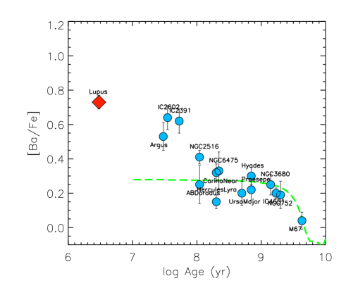
Figure 13: [Ba/Fe] abundance as a function of cluster age for dwarf stars in Lupus (this work) and other regions (from the literature). The red diamond represents the mean value of the most reliable Ba abundances obtained for the two warmest targets (see text and Table 2). Cluster abundances and ages were taken from D’Orazi et al. (2009, 2012), De Silva et al. (2013), and Reddy & Lambert (2015). The dashed line represents the Galactic chemical evolution model developed by D’Orazi et al. (2009) adopting enhanced $s$-process yields from AGB stars.

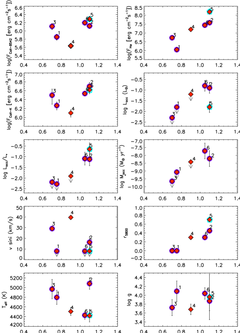
Figure 14: Dependence of the [Ba/Fe] abundance on activity (Ca ii-8542, H$\alpha$, Ca ii-K fluxes) and accretion ($L_{\rm acc}$, $L_{\rm acc}/L_{\star}$, $\dot{M}_{\rm acc}$, $r_{5800}$) diagnostics and on stellar parameters ($v\sin i$, $T_{\rm eff}$, $\log g$). Stars are enumerated: SSTc2d J160830.7-382827 (1), RY Lup (2), MY Lup (3), Sz 68 (4), Sz 133 (5), and SSTc2d J160836.2-392302 (6). Open circles and pentagons represent transitional disk and sub-luminous targets, respectively. Error bars of the [Ba/Fe] abundances are not plotted for clarity reasons.

5 Conclusions

We have presented the results of a study on elemental abundances in the Lupus star-forming region using spectroscopic data acquired with X-shooter at the VLT. The studied sample comprises of almost all class II objects in the Lupus I, II, III, and IV clouds (82 over 89 sources; see Alcalá et al. 2017) and seven class III objects. Three elements were analyzed: lithium, iron, and barium.

Our main results can be summarized as follows:

• We detected the lithium line at $\lambda$=6707.8 Å  in all targets but six. The class III object Sz 94 does not show any hint of the absorption line, while for the other five class II targets we could only measure upper limits for the lithium equivalent widths due to the low $S/N$ of the spectra.

• Three objects appear to be highly lithium depleted. They represent only a few percent of the Lupus population, hence they are extremely rare, as found in other star-forming regions. The depletion in the lithium elemental abundance observed in such objects is still not reproduced by pre-main sequence evolutionary models in the literature, which makes them appealing for future detailed studies.

• For six class II targets we measured iron and barium abundance through spectral synthesis. The mean iron abundance in the Lupus star-forming region is consistent, within the errors, with the chemical pattern of the Galactic thin disk in the solar neighborhood.

• We found enhancement in barium abundance up to $\sim 0.7$ dex level. Our targets thus confirm and extend to a younger age that previously found by other authors. We discussed several possible explanations for this puzzling behavior, including chromospheric and accretion effects, uncertainties in stellar parameters, and departure from LTE approximation, but none of these seems to completely justify the barium over-abundance. The barium problem is still an open issue and deserves further work, both theoretical and observational, in particular at cluster ages $\raisebox{-2.15277pt}{$\>\stackrel{{\scriptstyle\textstyle<}}{{\sim}}\>$}50$ Myr.