Finite element approximations of minimal surfaces: algorithms and mesh refinement

Abstract

Finite element approximations of minimal surface are not always precise. They can even sometimes completely collapse. In this paper, we provide a simple and inexpensive method, in terms of computational cost, to improve finite element approximations of minimal surfaces by local boundary mesh refinements. By highlighting the fact that a collapse is simply the limit case of a locally bad approximation, we show that our method can also be used to avoid the collapse of finite element approximations. We also extend the study of such approximations to partially free boundary problems and give a theorem for their convergence. Numerical examples showing improvements induced by the method are given throughout the paper.

Keywords

Minimal surfaces Finite element method Mesh refinement Plateau problem

AMS subject classifications

49Q05, 65N30

1 Introduction

Let $D=\left\{(u,v)\in\mathbb{R}^{2}\,\middle|\,u^{2}+v^{2}<1\right\}$ be the unit disk and $\partial D=S^{1}$ be its boundary. Let $\varphi:\overline{D}\to\mathbb{R}^{d}$ $(d\geq 2)$ be a map that is sufficiently smooth and $\operatorname{rank}D\varphi=2$ almost everywhere in $D$, where $D\varphi$ is the Jacobi matrix of $\varphi$. By this assumption, its image $\varphi(D)\subset\mathbb{R}^{d}$ is a two-dimensional surface, possibly with self-intersections. In this paper, we refer to the map as $\varphi$ and to the surface as $\varphi(D)$. If the mean curvature of $\varphi$ vanishes at each point on $\varphi(D)$, then $\varphi(D)$ is called a minimal surface.

Let $\Gamma\subset\mathbb{R}^{d}$ $(d\geq 2)$ be an arbitrary Jordan curve. That is, $\Gamma$ is the image of a continuous embedding of $\partial D$ into $\mathbb{R}^{d}$. We would like to find minimal surfaces $\varphi$ spanned in $\Gamma$, that is,

$$\varphi:\overline{D}\to\mathbb{R}^{d}\text{ with }\varphi(\partial D)=\Gamma.$$

For a given Jordan curve $\Gamma$, the problem of finding minimal surfaces spanned in $\Gamma$ is called the (classical) Plateau problem [2], [3], [7]. For the Plateau problem, the following variational principle has been known [2], [3]:
Define the subset $X_{\Gamma}$ of $C(\overline{D};\mathbb{R}^{d})\cap H^{1}(D;\mathbb{R}^{d})$ by

$$X_{\Gamma}:=\Bigl{\{}\psi\in C(\overline{D};\mathbb{R}^{d})\cap H^{1}(D;\mathbb{R}^{d})\Bigm{|}\psi(\partial D)=\Gamma\text{ and }\psi|_{\partial D}\text{ is monotone}\Bigr{\}},$$ (1)

where $\psi|_{\partial D}$ being monotone means that $(\psi|_{\partial D})^{-1}(p)$ is connected for any $p\in\Gamma$. Although $\psi|_{\partial D}$ has to be onto, it does not need to be one-to-one. We denote the Dirichlet integral (or the energy functional) on $D$ for $\varphi=(\varphi_{1},\cdots,\varphi_{d})^{\top}\in H^{1}(D;\mathbb{R}^{d})$ by

$$\mathscr{D}(\varphi):=\frac{1}{2}\int_{D}|\nabla\varphi|^{2}\mathrm{d}x=\frac{1}{2}\sum_{i=1}^{d}\int_{D}|\nabla\varphi_{i}|^{2}\mathrm{d}x.$$ (2)

Then, $\varphi\in X_{\Gamma}$ is a minimal surface if and only if $\varphi\in X_{\Gamma}$ is a stationary point of the functional $\mathscr{D}$ in $X_{\Gamma}$. Moreover, we have

$$\operatorname{Area}(\varphi(D))=\mathscr{D}(\varphi)=\inf_{\psi\in X_{\Gamma}}\mathscr{D}(\psi).$$

To obtain numerical approximations for the Plateau problem, the piecewise linear finite element method has been applied [10, 11, 12, 13, 14]. Firstly, functions of $X_{\Gamma}$ are approximated by piecewise linear functions on a triangulation of $D$. Then, starting from a suitable initial surface, stationary surfaces of the Dirichlet integral are computed by a relaxation procedure. This method has the advantage to be quite simple and straightforward to put in use. In the relaxation procedure, the images of inner nodes are moved $d$-dimensionally by, for example, Gauss-Seidel method, and the images of nodes on $\partial D$ are moved through $\Gamma$ by, for example, Newton method. See [10, Figure 1]. Because the images of nodes on $\partial D$ will move rather freely on $\Gamma$, finite element approximations can be very poor, sometimes even collapse, if the configuration of $\Gamma$ is not simple enough.

The first aim of this paper is to provide a technique to overcome this difficulty. We will present a straightforward adaptive mesh refinement algorithm that is almost inexpensive in terms of computational cost. The details of our refinement technique will be explained in Section 3.

The second aim of this paper is to extend the results of finite element (FE) minimal surfaces to the case of minimal surfaces with partially free boundary. Let a smooth surface $\mathscr{S}\subset\mathbb{R}^{d}$ be given. Suppose that $\Gamma\subset\mathbb{R}^{d}$ is now a piecewise smooth curve with end-points on $\mathscr{S}$. That is, $\Gamma$ is the image of a smooth map $\gamma:[-1,1]\to\mathbb{R}^{d}$ with $\gamma(-1),\gamma(1)\in\mathscr{S}$. We would like to find minimal surfaces $\varphi$ such that $\varphi(\partial D)\subset\Gamma\cup\mathscr{S}$. Note that the image of $\varphi$ on $\mathscr{S}$ is not known a priori. In Section 4, we will show that our methodology works well to obtain FE minimal surfaces with partially free boundary. We will also give a theorem for convergence of FE minimal surfaces.

In Section 5, we will discuss some useful data structures and specify a general algorithm to compute FE approximations with the method that will have been discussed.

To highlight the effectiveness of the proposed method, several numerical examples will be given throughout this paper.

2 Minimal surfaces

As explained in the previous section, in this paper, surfaces refer to mappings

$$\varphi:\Omega\to\mathbb{R}^{d},\qquad\varphi=(\varphi_{1},\cdots,\varphi_{d})^{\top},$$

from a bounded domain $\Omega\subset\mathbb{R}^{2}$ into $\mathbb{R}^{d}$ with $\operatorname{rank}D\varphi=2$. A point $p\in\Omega$ is always written as $p=(u,v)^{\top}$. The area functional $\mathscr{A}(\varphi)$ of the surface $\varphi$ is defined by

$$\mathscr{A}(\varphi)=\int_{\Omega}{}{\left|\varphi_{u}\wedge\varphi_{v}\right|}\mathrm{d}\mathbf{x},\qquad\mathrm{d}\mathbf{x}=\mathrm{d}{u}\mathrm{d}{v},$$

$$\varphi_{u}:=\left(\frac{\partial\varphi_{1}}{\partial u},\cdots,\frac{\partial\varphi_{d}}{\partial u}\right)^{\top},\quad\varphi_{v}:=\left(\frac{\partial\varphi_{1}}{\partial v},\cdots,\frac{\partial\varphi_{d}}{\partial v}\right)^{\top},$$

and stationary points of $\mathscr{A}$ are called minimal surfaces.

The stationary points of the area functional, and in particular, its minimizers, are the surfaces of zero mean curvature. In other words, a map is a minimal surface if and only if its mean curvature vanishes at any point on the surface.

We consider the Plateau problem. This problem is to find minimal surfaces mapping a bounded, 1-connected domain to a surface contoured by $\Gamma$. A domain is 1-connected (or simply-connected) is it is path-connected and if every path between two points can be continuously transformed into any other path with the same endpoints (informally, there is no “hole”). We may assume without loss of generality that $\Omega$ is the unit disk. In the sequel of this paper, we only consider the case $\Omega=D$.

The Belgian physicist Joseph Plateau made several experiments with soap films. In particular, he observed that when he dipped a frame consisting of a single closed wire into soapy water, it would always result in a soap surface spanned in the closed wire, whatever may be the geometrical form of the frame. From a mathematical point of view, the single closed wire is a Jordan curve, a curve topologically equivalent to the unit circle, and the resulting soap film is a surface in $\mathbb{R}^{3}$. From the theory of capillary surfaces, we know that the surface energy is proportional to its area. From these observations, one has good reasons to think that every (rectifiable) Jordan curve bounds at least one minimal surface. The Plateau problem is then first to show the existence of such surfaces. The problem has been solved for general contours by Douglas [4] and Radó [8].

Note that, for any $\psi\in X_{\Gamma}$, we have

$$\mathscr{A}(\psi)=\mathscr{A}(\psi\circ\eta)\quad\text{for an arbitrary diffemorphism }\;\eta:\overline{D}\to\overline{D}.$$

Hence, if we consider the Plateau problem with respect to the area functional $\mathscr{A}$, we would have to deal with the space of all diffeomorphisms on $\overline{\Omega}$. This was the main reason why the problem was so difficult to solve.

Later, the existence proof was significantly simplified by Courant. Courant pointed out that a map $\varphi:D\to\mathbb{R}^{d}$ is a minimal surface if and only if it is a stationary point of the Dirichlet integral (2) in $X_{\Gamma}$. Note that if a map $\varphi:\overline{D}\to\mathbb{R}^{d}$ is stationary in $X_{\Gamma}$, then it satisfies the following equations:

$$\Delta\varphi=\left(\Delta\varphi_{1},\cdots,\Delta\varphi_{d}\right)^{\top}=0\quad\text{ and }\left|\varphi_{u}\right|^{2}=\left|\varphi_{v}\right|^{2},\;\varphi_{u}\cdot\varphi_{v}=0\quad\text{ in }D.$$

The second and third equations mean that $\varphi$ is isothermal, or conformal.

Courant showed the following theorem [2, Chapter 3], [3, Main Theorem, p.270]:

Theorem 1.

There exists a map $\varphi\in X_{\Gamma}$ that attains the infimum of the Dirichlet integral in $X_{\Gamma}$, that is,

$$\mathscr{D}(\varphi)=\inf_{\psi\in X_{\Gamma}}\mathscr{D}(\psi).$$ (3)

This $\varphi$ is a solution to the Plateau problem.

The map which satisfies (3) is called the Douglas-Radó solution.

Note that, for any $\psi\in X_{\Gamma}$, we have

$$\mathscr{D}(\psi)=\mathscr{D}(\psi\circ\eta)\quad\text{for an arbitrary conformal map }\;\eta:\overline{D}\to\overline{D}.$$

Hence, if we consider the Plateau problem with respect to the Dirichlet integral $\mathscr{D}$, we only need to deal with the space of all conformal maps on $\overline{D}$. A conformal map $\eta:\overline{D}\to\overline{D}$ is determined uniquely by a normalization condition, which can be one of the following conditions:

• Assigning the image of three points $p_{i}\in\partial D$, $i=1,2,3$.

• Assigning the image of one inner point $p_{0}\in D$ and one boundary point $p_{1}\in\partial D$.

• Assigning the image of one inner point $p_{0}\in D$ and the direction of the derivative at $p_{0}$.

Thus, if we use one of these normalization conditions, a surface $\varphi\in X_{\Gamma}$ is (locally) “fixed”. This was the reason why Courant could simplify the Plateau problem so much.

In this paper, we deal with the first of these conditions, which can be applied to any dimension higher than two. For the sake of precision and notation, let us write it in more details, this time applied to our problem:
Take different points $p_{1},p_{2},p_{3}\in\partial D$ and $q_{1},q_{2},q_{3}\in\Gamma$. Then, impose $\varphi(p_{i})=q_{i},\,i=1,2,3$. Figure 1 illustrates this normalization condition.

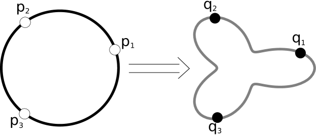
Figure 1: As a normalization condition, we fix the images of three points on the boundary $(d\geq 2)$

Let us summarize notation of function spaces we use in this paper. The set of all continuous functions on $\overline{D}$ with the uniform convergence metric is denoted by $C(\overline{D})$. The spaces $L^{2}(D)$ and $H^{1}(D)$ are defined by

$$L^{2}(D):=\left\{f:D\to\mathbb{R}\,\middle|\,\int_{D}{}{|f|^{2}}{x}<\infty\right\},$$

$$H^{1}(D):=\left\{f\in L^{2}(D)\,\middle|\,f_{u},f_{v}\in L^{2}(D)\right\}.$$

Their norms are also defined as usual. The set of maps $\varphi:D\to\mathbb{R}^{d}$ whose components belong, for example, to $L^{2}(D)$ is denoted by $L^{2}(D;\mathbb{R}^{d})$. The sets $C(\overline{D};\mathbb{R}^{d})$ and $H^{1}(D;\mathbb{R}^{d})$ are defined similarly.

3 Finite element approximation

In this section, we detail how to compute a FE approximation of the solution to the problem detailed in Section 2. We present a general method, highlight two problems that easily occur and propose a solution.

3.1 Definitions

Let $\mathcal{T}$ be a face-to-face triangulation of the unit disk $D$. This means that $\mathcal{T}$ is a set of triangles (which are regarded as closed sets) such that

• $\displaystyle D_{h}:=\bigcup_{K\in\mathcal{T}}K\subset\overline{D}$.

• If $K_{1}$, $K_{2}\in\mathcal{T}$ with $K_{1}\neq K_{2}$, then either $K_{1}\cap K_{2}=\emptyset$ or $K_{1}\cap K_{2}$ is a common vertex or a common edge of $K_{1}$ and $K_{2}$.

• $\partial D_{h}$ is a piecewise linear inscribed curve of $\partial D$.

For a triangulation $\mathcal{T}$, we define its fineness by $|\mathcal{T}|:=\max_{K\in\mathcal{T}}\operatorname{diam}K$.

Let $\mathcal{P}^{1}$ be the set of all polynomials with two variables of degree at most $1$. We introduce the set of piecewise linear functions on $\mathcal{T}$ as

$$S_{h}:=\left\{v_{h}\in C(D_{h})\bigm{|}v_{h}|_{K}\in\mathcal{P}^{1},\forall K\in\mathcal{T}\right\}.$$

Note that each $v_{h}\in S_{h}$ is defined only on $D_{h}\subset\overline{D}$. We extend each function $v_{h}\in S_{h}$ to $D\backslash D_{h}$ by the way described in [10]. That yields the inequalities

$$\|v_{h}\|_{H^{1}(D_{h})}\leq\|v_{h}\|_{H^{1}(D)}\leq(1+Ch)\|v_{h}\|_{H^{1}(D_{h})}.$$ (4)

Let $\mathcal{N}_{bdy}$ be the set of all nodes on $\partial D$. We define the discretization of $X_{\Gamma}$ by

$$X_{\Gamma_{h}}:=\Bigl{\{}\psi_{h}\in(S_{h})^{d}\Bigm{|}\psi_{h}(\mathcal{N}_{bdy})\subset\Gamma,\;\psi_{h}|_{\partial D}\text{ is }d\text{-monotone}\Bigr{\}},$$

where $\psi_{h}\in(S_{h})^{d}$ being $d$-monotone means that if $\partial D$ is traversed once in the positive direction, then $\Gamma$ is traversed once in a given direction, although we allow arcs of $\partial D$ to be mapped onto single points of $\Gamma$.

The triangulations we use for the different mappings of this paper are shown in Figure 2. This figure also gives which points of the triangulation are chosen to play the role of the points used as a normalization condition. For simplicity, we shall refer to these points as fixed points. Triangulation 1 has 169 interior nodes and 48 boundary nodes. Triangulation 2 has 331 interior nodes and 66 boundary nodes. Except for one exception in Figure 5, where we use $p_{1}$, $p^{\prime}_{2}$, and $p^{\prime}_{3}$, we always use as fixed points $p_{1}$, $p_{2}$, and $p_{3}$ such as indicated on the figures.

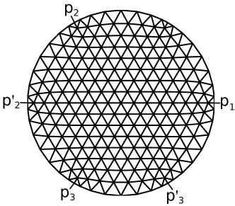
(a) Triangulation 1

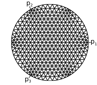
(b) Triangulation 2

Figure 2: The two triangulations used in this paper

Definition 1.

A stationary point $\varphi_{h}\in X_{\Gamma_{h}}$ of $\mathscr{D}$ is called a FE minimal surface spanned in $\Gamma$. In particular, a minimal surface $\varphi_{h}\in X_{\Gamma_{h}}$ such that

$$\mathscr{D}(\varphi_{h})=\inf_{\psi_{h}\in X_{\Gamma_{h}}}\mathscr{D}(\psi_{h})$$

is called FE Douglas-Radó solution.

From the definitions it is obvious that such solutions exist [11, Section 5].

To apply the three points condition, we take $p_{i}\in\partial D$ and $q_{i}\in\Gamma$, $i=1,2,3$, and fix them. In this paper, we always assume that $p_{i}\in\mathcal{N}_{bdy}$. We then define $X_{\Gamma}^{tp}$ and $X_{\Gamma_{h}}^{tp}$ by

$$X_{\Gamma}^{tp} :=\Bigl{\{}\psi\in X_{\Gamma}\Bigm{|}\psi(p_{i})=q_{i},\,i=1,2,3\Bigr{\}},$$

$$X_{\Gamma_{h}}^{tp} :=\Bigl{\{}\psi\in X_{\Gamma_{h}}\Bigm{|}\psi(p_{i})=q_{i},\,i=1,2,3\Bigr{\}}.$$

The suffix “$tp$” stands for the three points condition.

3.2 Convergence

For the convergence of FE minimal surfaces, the following theorems have been known [11], [12], [13]. Let $\{\mathcal{T}_{h}\}_{h>0}$ be a sequence of regular and quasi-uniform triangulations [1] of $D$ such that $\lim_{h\to 0}|\mathcal{T}_{h}|=0$, and $p_{i}$, $i=1,2,3$ are nodal points for any $\mathcal{T}_{h}$.

Theorem 2.

Suppose that $\Gamma$ is rectifiable. Let $\{\varphi_{h}\}_{h>0}$ be the sequence of FE Douglas-Radó solutions on $\mathcal{T}_{h}$. Then, there exists a subsequence $\{\varphi_{h_{i}}\}\subset X_{\Gamma_{h_{i}}}^{tp}$ which converges to one of the Douglas-Radó solution $\varphi\in X_{\Gamma}^{tp}$ spanned in $\Gamma$ in the following sense$:$

$$\lim_{h_{i}\to 0}\|\varphi_{h_{i}}-\varphi\|_{H^{1}(D;\mathbb{R}^{d})}=0,$$ (5)

and if $\varphi\in W^{1,p}(D;\mathbb{R}^{d})$, $p>2$, then

$$\lim_{h_{i}\to 0}\|\varphi_{h_{i}}-\varphi\|_{C(\overline{D};\mathbb{R}^{d})}=0.$$ (6)

A minimal surface $\varphi\in X_{\Gamma}^{tp}$ is said to be isolated and stable if there exists a constant $\delta$ such that

$$0<\|\varphi-\psi\|_{C(\overline{D};\mathbb{R}^{d})}<\delta\quad\text{ implies }\quad\mathscr{D}(\varphi)<\mathscr{D}(\psi)\quad\text{ for }\psi\in X_{\Gamma}^{tp}.$$

Theorem 3.

Suppose that $\Gamma$ is rectifiable. Let $\varphi\in X_{\Gamma}^{tp}$ be an isolated and stable minimal surface spanned in $\Gamma$. Then, there exists a sequence $\{\varphi_{h}\}_{h>0}$ of stable FE minimal surfaces which converges to $\varphi$ in the sense of (5) and (6).

Remark 1: Note that in [11, 12, 13], Theorems 2 and 3 were proved under the assumption that the triangulations $\{\mathcal{T}_{h}\}$ are regular, quasi-uniform, and non-negative type. As was pointed out in [13], however, the weak discrete maximum principle shown by Schatz [9] holds for discrete harmonic functions (maps) on regular, quasi-uniform triangulations [13, Lemma 2.1]. Therefore, we here do not need to assume non-negative-typeness of triangulations to show Theorems 2 and 3.

Dziuk and Hutchinson gave an error analysis of FE minimal surfaces under certain regularity assumptions on $\Gamma$. They claim that if $\varphi$ is a “nondegenerate” minimal surface spanned in $\Gamma$, then there exist FE minimal surfaces $\varphi_{h}\in X_{\Gamma}^{tp}$ such that

$$\|\varphi-\varphi_{h}\|_{H^{1}(D;\mathbb{R}^{d})}\leq Ch,$$

where $C$ is a constant independent of $h$. See [5], [6] for the details.

3.3 Boundary approximation of FE minimal surfaces

Let $\mathcal{T}$ be a face-to-face triangulation of $D$ and $\{(x_{i},y_{i})\}_{i=1}^{N}$ be the set of nodes of $\mathcal{T}$, where $N$ is the number of nodes. Let $\{\eta_{i}\}\subset S_{h}$ be the basis of $S_{h}$ defined by $\eta_{i}(x_{i},y_{i})=1$ and $\eta_{i}(x_{j},y_{j})=0$, for $i\neq j$. Then, a piecewise linear surface $\psi_{h}$ is expressed by $\psi_{h}=\sum_{i=1}^{N}\eta_{i}(a_{i,1},\cdots,a_{i,d})$, where $(a_{i,1},\cdots,a_{i,d})\in\mathbb{R}^{d}$ is the image of the point $(x_{i},y_{i})$ by $\psi_{h}$.

Moreover, its Dirichlet integral $\mathscr{D}(\psi_{h})$ is written as

$$\mathscr{D}(\psi_{h})=\frac{1}{2}\int_{D}|\nabla\psi_{h}|^{2}\mathrm{d}x=\frac{1}{2}\left(a_{1}^{\top}\widetilde{A}a_{1}+\cdots+a_{d}^{\top}\widetilde{A}a_{d}\right),$$ (7)

where

$$a_{k}=(a_{1,k},\cdots,a_{N,k})^{\top}\in\mathbb{R}^{N},\quad k=1,\cdots,d,$$

$$\widetilde{A}=\left(\alpha_{ij}\right)_{i,j=1,\cdots,N},\quad\alpha_{ij}:=\int_{D}\nabla\eta_{i}\cdot\nabla\eta_{j}\mathrm{d}x.$$

We would like to find a stationary point $\varphi_{h}$ of $\mathscr{D}$ in $X_{\Gamma_{h}}^{tp}$. Recall that, if $\psi_{h}\in X_{\Gamma_{h}}^{tp}$, then $\psi_{h}(\mathcal{N}_{bdy})\subset\Gamma$. This means that, if $(x_{i},y_{i})\in\mathcal{N}_{bdy}$, $\psi_{h}(x_{i},y_{i})$ should be on $\Gamma$. Suppose that $\Gamma$ is parametrized by a parameter $t\in[0,2\pi]$ as $\Gamma(t)=(\gamma_{1}(t),\cdots,\gamma_{d}(t))$. Then, if $\psi_{h}(x_{i},y_{i})\in\Gamma$, $\psi_{h}(x_{i},y_{i})$ is written as

$$\psi_{h}(x_{i},y_{i})=(a_{i,1}\eta_{i}(x_{i},y_{i}),\cdots,a_{d,i}\eta_{i}(x_{i},y_{i}))=(a_{i,1},\cdots,a_{d,i})=(\gamma_{1}(t_{i}),\cdots,\gamma_{d}(t_{i}))$$ (8)

for some $t_{i}\in[0,2\pi]$.

We apply a relaxation procedure to find a stationary point $\varphi_{h}\in X_{\Gamma_{h}}^{tp}$. That is, to find a stationary point of $\mathscr{D}(\psi_{h})$, only one vector $(a_{i,1},\cdots,a_{i,d})$ is updated at each step. To apply the relaxation procedure to $\mathscr{D}(\psi_{h})$, we have to consider two cases.

Case 1: $(x_{i},y_{i})$ is in the interior of $D$. In this case, because $\mathscr{D}(\psi_{h})$ is a quadratic function with respect to $a_{i,k}$ and

$$\frac{\partial\;}{\partial a_{i,k}}\left(\frac{1}{2}a_{k}^{\top}Aa_{k}\right)=\sum_{j=1}^{N}\alpha_{ij}a_{j,k},\quad k=1,\cdots,d,$$

we may use, for example, simple Gauss-Seidel iteration

$$a_{i,k}^{(new)}:=-\sum_{j=1,j\neq i}^{N}\frac{\alpha_{ij}}{\alpha_{ii}}a_{j,k}^{(old)},\qquad k=1,\cdots,d.$$

Case 2: $(x_{i},y_{i})$ is on the boundary of $D$. In this case, the relaxation procedure becomes more complicated. We insert (2) into (1), and $\mathscr{D}(\psi_{h})$ may be written as

$$F(t_{i}):=\mathscr{D}(\psi_{h}),\quad t_{i}\in[0,2\pi]$$

in the relaxation step at a boundary node. We would like to find $t_{i}$ such that $F^{\prime}(t_{i})=0$ at all boundary nodes $(x_{i},y_{i})$. To this end, we employ the Newton method

$$t_{i}^{(new)}:=t_{i}^{(old)}-\frac{F^{\prime}(t_{i}^{(old)})}{F^{\prime\prime}(t_{i}^{(old)})}.$$

At first, images of the points on $\partial D$ are distributed with equal intervals on $\Gamma$ with respect to the positions of the three fixed points. In the optimization process, boundary point images $\varphi_{h}(\mathcal{N}_{bdy})$ move rather freely on $\Gamma$. As a result, we might have a FE minimal surface with a poor approximation of $\Gamma$, if the cardinality of $\mathcal{N}_{bdy}$ is not large enough. Figure 3(a) illustrates such a situation. The parametric equation of the curve represented is

$$\begin{cases}x=(1+0.5\cos{3\theta})*\cos(\theta),\\ y=(1+0.5\cos{3\theta})*\sin(\theta),\end{cases}$$

and it looks like the one on the right side of Figure 1.

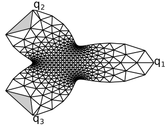
(a) Poor approximation of some parts of the domain (obtained in 806 iterations)

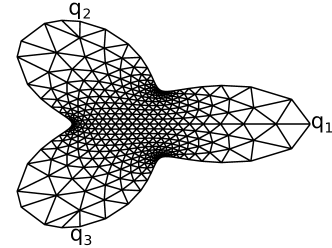
(b) Better approximation obtained by adding four boundary points on defective triangles (obtained in 897 iterations)

Figure 3: Comparison of two approximations of the same curve

A simple naive way to obtain a better approximation is of course to use a finer triangulation of the unit disk so that $\varphi_{h}(\mathcal{N}_{bdy})$ provides a better approximation of $\Gamma$.

Our simple and effective method consists of dynamical insertions of boundary nodes on triangles whose images are “defective”. A triangle is called a boundary triangle, if two of its vertices belong to $\mathcal{N}_{bdy}$, and the image of a boundary triangle is said to be defective if the distance (or the angle) between these two vertices is much larger than the one of its neighbour triangles. Let choose a positive integer $C$. Every $C$ iterations of the relaxation process, we check the quality of the boundary. When a defective triangle is identified, we split its inverse image into two smaller triangles by inserting a new boundary node at the middle of its boundary arc (the arc of circle between its two boundary nodes) and joining this node to the vertex facing it, before continuing the relaxation process. Adding few boundary points to defective triangles during the relaxation process, we can get a better approximation, as shown by Figure 3(b).

An even more problematic situation can occur, when the approximation completely collapses, as shown by Figure 4(a). This case can be viewed as an extreme case of the previous one. Such a situation would happen if a triangle becomes much larger than its neighbourhood, resulting in its collapse. It can therefore be overcome by the method described above, as shown by Figure 4(b). We see a limitation of such an adaptive bisection method. The computation is hindered by the insertion of too many points. Figure 4(c) shows the result of the same adaptive method but this time combined with a different refinement technique. A defective boundary triangle is split into four triangles by joining the middle points of its three edges. Such a refinement technique is often called regular refinement and the previous one marked edge bisection (see [15, Section 4.1]. The regular refinement has the advantage to produce triangles that are similar to the one from which they are created. On the other hand it involves a more complex and heavier computation as the technique introduces hanging nodes — nodal points in the middle of an edge — on the neighbours of the refined triangle. To preserve the triangulation, a hanging node is joined to the vertex facing it.

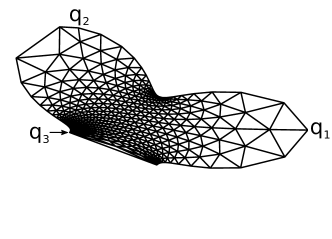
(a) The approximation collapses due to the choices of the fixed points and their images

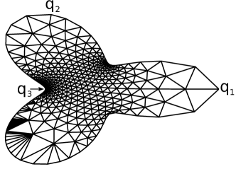
(b) The approximation is restored by bisecting defective triangles

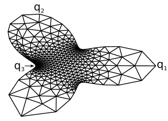
(c) The approximation is restored by regularly refining defective triangles

Figure 4: An example of approximation that collapses and how it can be restored

3.4 A $3-$dimensional example

We provide another example of how the described method allows to avoid the collapse of the approximation, this time in three dimensions. We use Triangulation 1 to map the unit circle to the curve defined by

$$\begin{cases}x=\cos\theta(1+0.5*\sin(2\theta)),\\ y=\sin\theta(1+0.5*\sin(2\theta)),\\ z=0.5\sin(3\theta).\end{cases}$$

We see in Figure 5(a) that the original approximation makes the boundary (the grey curve) impossible to recognize. Figure 5(b) shows the approximation obtained by adaptive regular refinements on defective boundary triangles. We may want to see how the approximation behaves if we choose different fixed points. Instead of $p_{1}$, $p_{2}$, and $p_{3}$, we now choose $p_{1}$, $p^{\prime}_{2}$, and $p^{\prime}_{3}$ such as defined in Figure 2(a). Note that the choice of these points is arbitrary and serves no other purpose than to illustrate the fact that collapsed approximations are very common. Figures 5(c) shows that, without inserting nodes, we get a better approximation than the previous one, but a part of the curve is still missing. By the same method, we once again avoid the collapse and get a good approximation, as shown by Figure 5(d). Note that even if we greatly improve the approximation, there may sometimes remain some areas that are still poorly approximated such as the sharp peak we can see in the figure. This can generally be solved by increasing the number of points in the triangulation (Figure 5(e) shows the result of our method applied to map Triangulation 2) or by locally refining, after the initial mapping, the problematic areas to better approximate the surface and its boundary (a posteriori refinement).

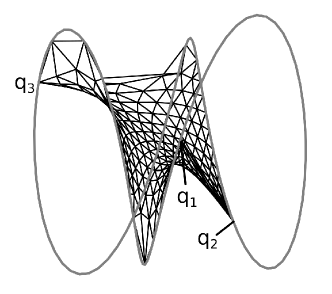
(a) The original approximation has collapsed

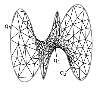
(b) 16 insertions to obtain a good approximation

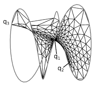
(c) The same example with different fixed points

(d) 32 insertions to improve the approximation

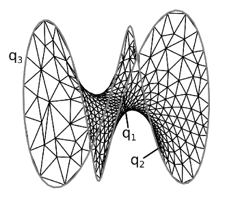
(e) Increasing the number of nodes in the triangulation

Figure 5: A $3-$dimensional example

3.5 Approximating corners

Such an adaptive mesh refinement method is particularly effective to handle curves with several corners. Approximations of corners by piecewise elements are often mediocre. If the curve has less than four corners, these can be chosen as fixed images and the approximation can stay unspoiled. However, if the number of corners is higher, one has to find a way to approximate them better. Let us take the example of the square $[-1,1]\times[-1,1]$. One possibility is to use a smoothing function [13], but we show in Figure 6 how the approximation at the corner can be improved by the described method (here, we used bisections). The nodes on the edge of the bottom right corner have coordinates $(0.59,-1.0)$, $(1.0,-0.62)$ in Figure 6(a), and $(0.86,-1.0)$, $(1.0,-0.88)$ in Figure 6(b).

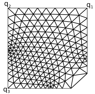
(a) Approximation of the square

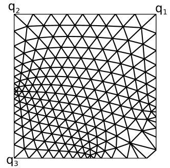
(b) 4 points inserted

Figure 6: An approximation of the $[-1,1]\times[-1,1]$ square

4 Partially free boundary

We now consider another problem that is to find a minimal surface with a partially free boundary. In this problem, the boundary to which we map the circle consists of the couple $\langle\Gamma,\mathscr{S}\rangle$ where $\mathscr{S}$ is a given closed surface in $\mathbb{R}^{3}$ and $\Gamma$ is a curve now connected to $\mathscr{S}$ by two points $q_{1}$ and $q_{3}$. If the mappings presented in Section 2 can be physically imagined as wire frames pulled out of soapy water, the ones presented from now on can be seen as the film created between the wire and an object connected to it. Note that the surface of the soapy water itself can be such an object. This case represents the situation while we are pulling the frame out from the water.

Note that $\langle\Gamma,\mathscr{S}\rangle$ can be modeled in different ways. One way is that $\Gamma$ is an open curve whose ending points lie on $\mathscr{S}$. The other way is that one part of the closed curve $\Gamma$ is “merged” into $\mathscr{S}$. In this model, we shall refer to the points on that part of the curve as surface points. Note that we refer to $\mathscr{S}$ as “surface” since it is easily physically represented by any surface, but it is of course in no case related to the minimal surface we are looking for.

As an illustration, we give a numerical example of a minimal surface with partially free boundary in Figure 7. In the example, $\Gamma$ is a part of a circle in $\mathbb{R}^{3}$ and $\mathscr{S}$ is (a convex bounded subset of) a plane.

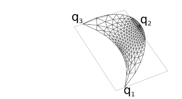
(a) $\Gamma$ is a small arc

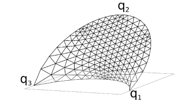
(b) $\Gamma$ is a bigger arc of the same circle

Figure 7: An example of minimal surface with partially free boundary

We now define the problem rigorously. Let $\Xi^{1}\subset\partial D$ be the closed interval of $\partial D$ such that $p_{2}\in\Xi^{1}$ and its end-points are $p_{1}$ and $p_{3}$. Set $\Xi^{2}:=\partial D\backslash\Xi^{1}$. We consider the following conditions for $\psi\in H^{1}(D;\mathbb{R}^{3})$:

• $\psi|_{\Xi^{2}}(w)\in\mathscr{S}$ for almost all $w\in\Xi^{2}$.

• $\psi|_{\Xi^{1}}$ is continuous and monotone on $\Xi^{1}$ such that $\psi(\Xi^{1})=\Gamma$ and $\psi(p_{i})=q_{i}$, $i=1,3$.

Here, $\psi|_{\Xi^{i}}$ is the trace of $\psi$ on $\Xi^{i}$, $i=1,2$. Then, the subset $X_{\langle\Gamma,\mathscr{S}\rangle}$ is defined by

$$X_{\langle\Gamma,\mathscr{S}\rangle}:=\Bigl{\{}\psi\in H^{1}(D;\mathbb{R}^{3})\Bigm{|}\text{$\psi$ satisfies (i) and (ii)}\Bigr{\}}.$$

As is stated, we suppose that $\Gamma$ is connected to $\mathscr{S}$ by $q_{1}$ and $q_{3}$, that is, $\Gamma\cap\mathscr{S}=\{q_{1},q_{3}\}$. Note that we have $\psi(p_{i})=q_{i}$, $i=1,3$ for $\psi\in X_{\langle\Gamma,\mathscr{S}\rangle}$ by the definition. We take $q_{2}\in\Gamma$ and define

$$X_{\langle\Gamma,\mathscr{S}\rangle}^{tp}:=\Bigl{\{}\psi\in X_{\langle\Gamma,\mathscr{S}\rangle}\Bigm{|}\psi(p_{2})=q_{2}\Bigr{\}}.$$

Then, as before, $\varphi\in X_{\langle\Gamma,\mathscr{S}\rangle}^{tp}$ is a minimal surface if and only if $\varphi$ is a stationary point of $\mathscr{D}$ in $X_{\langle\Gamma,\mathscr{S}\rangle}$. If $X_{\langle\Gamma,\mathscr{S}\rangle}^{tp}$ is not empty, there exists a minimal surface in $X_{\langle\Gamma,\mathscr{S}\rangle}^{tp}$ that attains the infimum of the Dirichlet integral in $X_{\langle\Gamma,\mathscr{S}\rangle}^{tp}$. Again, that minimal surface is called the Douglas-Radó solution. For the proof of existence of the Douglas-Radó solution, see [3, Theorem 2, p.278].

The FE approximation of minimal surfaces with partially free boundary is now almost obvious. Define the subsets of $\mathcal{N}_{bdy}$

$$\mathcal{N}_{bdy}^{1}:=\{p\in\mathcal{N}_{bdy}:p\in\Xi^{1}\},\qquad\mathcal{N}_{bdy}^{2}:=\mathcal{N}_{bdy}\backslash\mathcal{N}_{bdy}^{1},$$

and the discretizations of $X_{\langle\Gamma,\mathscr{S}\rangle}$ and $X_{\langle\Gamma,\mathscr{S}\rangle}^{tp}$ are defined by

$$X_{\langle\Gamma,\mathscr{S}\rangle,h} :=\Bigl{\{}\psi\in(S_{h})^{d}\Bigm{|} \psi(\mathcal{N}_{bdy}^{1})\subset\Gamma,\;\psi|_{\Xi^{1}}\text{ is $d$-monotone},$$

$$\psi(\mathcal{N}_{bdy}^{2})\subset\mathscr{S},\;\psi(p_{i})=q_{i},i=1,3\Bigr{\}},$$

$$X_{\langle\Gamma,\mathscr{S}\rangle,h}^{tp} :=\Bigl{\{}\psi\in X_{\langle\Gamma,\mathscr{S}\rangle}\Bigm{|} \enspace\psi(p_{2})=q_{2}\Bigr{\}}.$$

Stationary points in $X_{\langle\Gamma,\mathscr{S}\rangle,h}^{tp}$ with respect to the Dirichlet integral $\mathscr{D}$ are called $FE$ minimal surfaces with free boundary on $\mathscr{S}$. In particular, the minimizer of the Dirichlet integral in $X_{\langle\Gamma,\mathscr{S}\rangle,h}^{tp}$ is called FE Douglas-Radó solution.

For convergence, we have the following theorem:

Theorem 4.

Suppose that $\langle\Gamma,\mathscr{S}\rangle$ satisfies the following conditions:

• $\Gamma$ is rectifiable,

• $\mathscr{S}$ is a bounded closed subset of a plane in $\mathbb{R}^{3}$,

• $\Gamma\cap\mathscr{S}=\{q_{1},q_{3}\}$ and there is a rectifiable arc in $\mathscr{S}$ connecting $q_{1}$ and $q_{3}$.

Note that if $\langle\Gamma,\mathscr{S}\rangle$ satisfies the above conditions, $X_{\langle\Gamma,\mathscr{S}\rangle}^{tp}$ is nonempty [3, Theorem 2, p.278]. Suppose also that all the Douglas-Radó solutions spanned in $\langle\Gamma,\mathscr{S}\rangle$ belong to $C(\overline{D};\mathbb{R}^{3})\cap H^{1}(D;\mathbb{R}^{3})$.

Let $\{\varphi_{h}\}_{h>0}$ be the sequence of FE Douglas-Radó solutions on triangulation $\mathcal{T}_{h}$ such that $\varphi_{h}\in X_{\langle\Gamma,\mathscr{S}\rangle,h}^{tp}$ and $|\mathcal{T}_{h}|\to 0$ as $h\to 0$. Then, there exists a subsequence $\{\varphi_{h_{i}}\}\subset X_{\langle\Gamma,\mathscr{S}\rangle,{h_{i}}}^{tp}$ which converges to one of the Douglas-Radó solution $\varphi\in X_{\langle\Gamma,\mathscr{S}\rangle}^{tp}$ spanned in $\langle\Gamma,\mathscr{S}\rangle$ in the following sense$:$

$$\lim_{h_{i}\to 0}\|\varphi_{h_{i}}-\varphi\|_{H^{1}(D;\mathbb{R}^{3})}=0,$$ (9)

and if $\varphi\in W^{1,p}(D;\mathbb{R}^{3})$, $p>2$, then

$$\lim_{h_{i}\to 0}\|\varphi_{h_{i}}-\varphi\|_{C(D\cup\mathscr{C};\mathbb{R}^{3})}=0,$$ (10)

where $\mathscr{C}\subset\Xi^{1}$ is an arbitrary open arc contained in $\Xi^{1}$. If the Douglas-Radó solution is unique, then $\{\varphi_{h}\}$ converges to $\varphi$ in the sense of (9) and (10).

Proof.

Let $\varphi\in X_{\langle\Gamma,\mathscr{S}\rangle}^{tp}$ be one of the Douglas-Radó solution and let $\eta_{h}\in(S_{h})^{3}$ be the FE solution such that

$$\int_{D}\nabla\eta_{h}\cdot\nabla\mathbf{v}_{h}\mathrm{d}x=0,\quad\forall\mathbf{v}_{h}\in(S_{h})^{3},\quad\mathbf{v}_{h}|_{\partial D}=0,$$

with $\varphi(x)=\eta_{h}(x)$ for all $x\in\mathcal{N}_{bdy}$.

With the inequalities (4), we can modify the proof of [1, Theorem3.2.3] and prove that $\lim_{h\to 0}\|\varphi-\eta_{h}\|_{H^{1}(D)}=0$.

By the definition of FE Douglas-Radó solutions, we have $\mathscr{D}(\varphi_{h})\leq\mathscr{D}(\eta_{h})$, and hence $\mathscr{D}(\varphi_{h})$ is uniformly bounded. Also, $\|\varphi_{h}\|_{L^{2}(D)}$ is bounded because of the (discretized) maximum principle. Thus, $\|\varphi_{h}\|_{H^{1}(D)}$ is bounded, and there exists a subsequence $\{\varphi_{h_{i}}\}$ that converges weakly in $H^{1}(D;\mathbb{R}^{3})$ to some $\psi\in H^{1}(D;\mathbb{R}^{3})$. In the following, we show that $\psi$ belongs to $X_{\langle\Gamma,\mathscr{S}\rangle}^{tp}$ and is one of the Douglas-Radó solution.

By the lower-semicontinuity of the Dirichlet integral with respect to weak convergence in $H^{1}(D;\mathbb{R}^{3})$ that is shown in the proof of Theorem 1 [3, p.276], we have

$$\mathscr{D}(\psi)\leq\liminf_{h_{i}\to 0}\mathscr{D}(\varphi_{h_{i}})\leq\lim_{h_{i}\to 0}\mathscr{D}(\eta_{h_{i}})=\mathscr{D}(\varphi).$$

The last equality follows from the fact $\lim_{h\to 0}\|\varphi-\eta_{h}\|_{H^{1}(D)}=0$. Hence, if $\psi\in X_{\langle\Gamma,\mathscr{S}\rangle}^{tp}$, we conclude that $\psi$ is one of the Douglas-Radó solutions.

Because $\varphi_{h_{i}}$ converges weakly in $H^{1}(D;\mathbb{R}^{3})$ to $\psi$, we have

$$\lim_{h_{i}\to 0}\|\varphi_{h_{i}}-\psi\|_{L^{2}(D;\mathbb{R}^{3})}=0,\qquad\lim_{h_{i}\to 0}\|\varphi_{h_{i}}|_{\partial D}-\psi|_{\partial D}\|_{L^{2}(\partial D;\mathbb{R}^{3})}=0$$ (11)

by Rellish’s theorem, where $\varphi_{h_{i}}|_{\partial D}$ and $\psi|_{\partial D}$ are the traces of $\varphi_{h_{i}}$ and $\psi$ on $\partial D$.

$\varphi_{h_{i}}(\Xi^{1})$ is a polygonal curve approximating $\Gamma$ ***AND*** Applying [12, Lemma 3] to $\varphi_{h_{i}}(\Xi^{1})$, we notice that $\varphi_{h_{i}}(\Xi^{1})$ converges uniformly to $\Gamma$ as $h_{i}\to 0$. Hence, $\psi|_{\Xi^{1}}$ is continuous and monotone such that $\psi(\Xi^{1})$ with $\psi(p_{i})=q_{i}$, $i=1,2,3$.

By the assumptions on $\mathscr{S}$, $\mathscr{S}$ is a subset of a plane and $\varphi_{h_{i}}|_{\Xi^{2}}$ is a polygonal curve satisfying $\varphi_{h_{i}}(\mathcal{N}_{bdy}^{2})\subset\mathscr{S}$. Therefore, we have $\varphi_{h_{i}}|_{\Xi^{2}}\subset\mathscr{S}$. Because of (11), we have $\psi|_{\Xi^{2}}(w)\in\mathscr{S}$ for almost all $w\in\Xi^{2}$. Therefore, we conclude with $\psi\in X_{\langle\Gamma,\mathscr{S}\rangle}^{tp}$ and the proof is completed. $\square$ ∎

The condition on $\mathscr{S}$ is rather restrictive. The authors hope the condition will be weakened in future.

5 Data structures and algorithm

The implementation of data structures for finite element methods and mesh refinement depends on several things, among which:

• The computational object at the center of the computation. There are usually two choices: nodes or elements of the triangulation. The main difference is that the latter being composed of the former, either way, one need a strategy to go from nodes to elements and vice versa.

• The type of elements we deal with. In this paper, they are triangular elements.

• The refinement strategies, that is to say when and how refinement(s) occur: during the computation or a posteriori? Is it a bisection or a regular refinement?

Therefore, we describe, as an example, the choice we made for our own computation but it is left to the discretion of the reader to see if this fits their needs.

Our method is element-oriented (i.e. our computation treats triangles as the main objects). The nodes of the triangulation are ordered in a certain way. Accordingly, to each node corresponds an index. We refer to this index as the global index. However, since our method is element-oriented, we store this information as part of the information about elements. Therefore, we define an array elements describing the list of elements, in which, for $j=1,2,3$,

elements[i,j] = global index of the $j$th node of element $i$.

As the boundary is a special part, different from its mapped interior, we establish an ordered list of boundary nodes, so we have

boundary[i] = global index of the $i$th node of the boundary.

Hence we can say that the node with global index boundary[i] has boundary index $i$.

To indicate the location of the node with global index $i$, we use an array status, whose size is the number of nodes in the triangulation, and is at first initialized by

$$\texttt{status[i] =}\begin{cases}0&\mbox{if node }i\mbox{ is an interior node},\\ \mbox{its boundary index}&\mbox{if }i\mbox{ is a boundary point},\end{cases}$$

which is modified by

$$\texttt{status[i] =}\begin{cases}-\texttt{status[i]}&\mbox{if }i\mbox{ is a fixed point},\\ \texttt{status[i]}+\mathbf{card}(\mathcal{N}_{bdy})&\mbox{if }i\mbox{ is a free boundary node}.\end{cases}$$

For some refinement algorithms, error estimation, or problems that ask, for example, search of triangles having common nodes, it is very useful to implement the relation between neighbour triangles. This is the case for the regular refinement strategy. To do so, we use an array neighbours where, for $j=1,2,3$,

$$\texttt{neighbours[i,j] =}\begin{cases}k&\mbox{if triangle }k\mbox{ is neighbour to triangle }i\\ &\mbox{and }j\mbox{th node of }i\mbox{ is not common to }i\mbox{ and }k,\\ -1&\mbox{if the edge opposite to }j\mbox{th node of }i\mbox{ is part of the boundary}.\end{cases}$$

The neighbourhood relation is illustrated by Figure 8.

Finally, we need a structure for the matrix to which we apply the relaxation procedure. For the problem of this paper, a large part of this matrix is filled by zeros. Consequently, a list of lists that contains only the necessary values for each element is preferable to a full $2$-dimensional matrix.

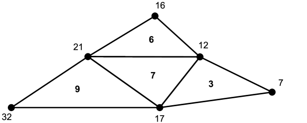
Figure 8: The neighbourhood of triangle $7$. elements$[7]=[21,17,12]$ so neighbours$[7]=[3,6,9]$

Algorithm 1 presents an overview of how the method is applied.

Algorithm 1 Relaxation process

1:elements, boundary, node_status, neighbours, functions describing $\Gamma$, global matrix

2:

3:$count\leftarrow 0$

4:$C\leftarrow$ number of iterations between two quality checks of the boundary

5:repeat

6:     if $count\equiv 0\pmod{C}$ then

7:         checkTriangles      

8:     for $i:1\to$ number of nodes do

9:         if $status[i]<0$ then      # fixed point

10:              continue

11:         else if $status[i]==0$ then      # inner point

12:              Relaxation by Gauss-Seidel method

13:         else if $status[i]>0$ then      # boundary node

14:              Relaxation by Newton method

15:              if $status[i]>\mathbf{card}(\mathcal{N}_{bdy})$ then      # free boundary node

16:                  Project node on surface.                             

17:     $count\leftarrow count+1$

18:until being under the relaxation tolerance threshold

19:

20:procedure checkTriangles

21:     for $i:1\to$ number of boundary nodes do

22:         if Criterion for insertion is met then

23:              $ele\leftarrow$ element containing $boundary[i]$ and $boundary[i+1]$

24:              Bisection($ele$)

25:              or

26:              RegularRefinement($ele$)               

27:Finite element approximation of the desired minimal surface

6 Conclusion

The refinement method presented in this paper has two main advantages.

First, it reduces the impact of the initial choices of the fixed points and their images. One can choose those in any way they want, the approximation obtained will never be collapsed and it will be close to the original contour.

Second, it allows us to reduce the number of nodes in the initial triangulation. As examples showed, it is not always necessary to substantially increase the number of nodes of the initial triangulation to obtain a good enough approximation. The described method refines the boundary very locally so only a necessary amount of points is inserted.

In the future, we will study how this simple method can be helpful to tackle more complex problems. We extended our study of finite element approximations to minimal surfaces with partially free boundary and we hope that the restrictions for the proof of convergence can be reduce. We will study partially free boundary problems with more complex surfaces than planar ones and we will challenge the Douglas-Plateau problem, where one looks for a minimal surface spanned in a system of several Jordan curves, such as a pyramid or a cube.

References

- [1] Ciarlet, P.: The Finite Element Method for Elliptic Problems. North Holland (1978). Reprinted by SIAM (2002)
- [2] Courant, R.: Dirichlet’s Principle, Conformal Mapping, and Minimal Surfaces. Interscience (1950). Reprinted by Springer (1997), reprinted by Dover (2005)
- [3] Dierkes, U., Hildebrandt, S., Sauvigny, F.: Minimal Surfaces, Grundlehren der mathematischen Wissenschaften, vol. 339. Springer-Verlag Berlin Heidelberg (2010)
- [4] Douglas, J.: Solution of the problem of plateau. Trans. Amer. Math. Soc. 33(1), 263–321 (1931). DOI 10.1090/S0002-9947-1931-1501590-9
- [5] Dziuk, G., Hutchinson, J.: The discrete plateau problem: Algorithm and numerics. Math. Comput. 68, 1–23 (1999). DOI 10.1090/S0025-5718-99-01025-X
- [6] Dziuk, G., Hutchinson, J.: The discrete plateau problem: convergence results. Math. Comput. 68, 519–546 (1999). DOI 10.1090/S0025-5718-99-01026-1
- [7] Osserman, R.: A Survey of Minimal Surfaces. Dover (2014)
- [8] Radó, T.: The problem of the least area and the problem of plateau. Math. Z. 32, 763–796 (1930)
- [9] Schatz, A.: A weak discrete maximum principle and stability of the finite element method in on plane polygonal domains. I. Math. Comput. 34(149), 77–91 (1980). DOI 10.2307/2006221
- [10] Tsuchiya, T.: On two methods for approximating minimal surfaces in parametric form. Math. Comput. 46, 517–529 (1986). DOI 10.2307/2007990
- [11] Tsuchiya, T.: Discrete solution of the plateau problem and its convergence. Math. Comput. 49, 157–165 (1987). DOI 10.2307/2008255
- [12] Tsuchiya, T.: A note on discrete solutions of the plateau problem. Math. Comput. 54, 131–138 (1990). DOI 10.2307/2008685
- [13] Tsuchiya, T.: Finite element approximations of conformal mappings. Numer. Func. Anal. Opt. 22, 419–440 (2001). DOI 10.1081/NFA-100105111
- [14] Tsuchiya, T.: Finite element approximations of conformal mappings to unbounded jordan domains. Numer. Func. Anal. Opt. 35, 1382–1397 (2014). DOI 10.1080/01630563.2013.837482
- [15] Verfürth, R.: A review of a posteriori error estimation and adaptive mesh-refinement techniques. Wiley Teubner (1996)