1. Introduction
Two-phase elastic membranes, consisting of coexisting fluid domains,
have received a lot of attention in the last 20 years. The interest in
two-phase membranes in particular was triggered by the multitude of
different shapes observed in experiments with inhomogeneous
biomembranes and vesicles. Biomembranes are typically formed as a
lipid bilayer, and often multiple lipid components are involved, which
laterally can separate into coexisting phases with different
properties. Among the complex morphologies that appear are micro-domains, which
resemble lipid rafts, and these are of huge interest in biology and
medicine. As the thickness of the membrane is much smaller than its
lateral length scale, typically the membrane is modelled as a
two-dimensional hypersurface in three dimensional Euclidean
space. The equilibrium shape of the membrane is obtained by minimizing an
energy which –besides other contributions– contains bending energies
involving the mean curvature and the Gaussian curvature of the
membrane. If different phases occur, parameters in the curvature energy
are inhomogeneous, leading to an interesting free boundary problem as
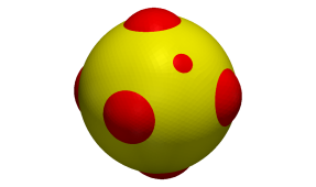
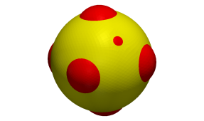
well as to a plethora of different shapes. We refer to
[12 ] , where multi-component giant unilamellar
vesicles (GUVs) separating into different phases were studied.
These authors were
able to optically resolve interactions between the different phases, its
curvature elasticity and the line tension of its interface.
There have been several studies on theoretical and numerical aspects
of two-phase membranes taking curvature elasticity and line energy
into account, see e.g. [28 , 29 , 39 , 11 , 40 , 15 , 30 , 22 , 23 , 24 , 25 , 26 , 13 , 32 , 14 , 9 ] ,
which we discuss in the following.
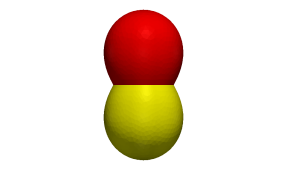
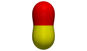
The by now classical model for a one-phase membrane rests on the
Canham–Helfrich–Evans elastic bending energy
1 2 α ∫ Γ ( ϰ − ϰ ¯ ) 2 d ℋ 2 + α G ∫ Γ 𝒦 d ℋ 2 , 1 2 𝛼 subscript Γ superscript italic-ϰ ¯ italic-ϰ 2 differential-d superscript ℋ 2 superscript 𝛼 𝐺 subscript Γ 𝒦 differential-d superscript ℋ 2 \tfrac{1}{2}\,\alpha\,\int_{\Gamma}(\varkappa-{\overline{\varkappa}})^{2}\;{\rm d}{\mathcal{H}}^{2}+\alpha^{G}\,\int_{\Gamma}{\mathcal{K}}\;{\rm d}{\mathcal{H}}^{2}\,,
where Γ Γ \Gamma ℋ 2 superscript ℋ 2 \mathcal{H}^{2} Γ Γ \Gamma ϰ italic-ϰ \varkappa 𝒦 𝒦 {\mathcal{K}} α 𝛼 \alpha α G superscript 𝛼 𝐺 \alpha^{G} ϰ ¯ ¯ italic-ϰ {\overline{\varkappa}}
In a fundamental work, Jülicher and Lipowsky
([28 , 29 ] ) generalized the
Canham–Helfrich–Evans model to two-phase membranes. The geometry is
now given by two smooth surfaces Γ 1 subscript Γ 1 \Gamma_{1} Γ 2 subscript Γ 2 \Gamma_{2} γ 𝛾 \gamma α 𝛼 \alpha α G superscript 𝛼 𝐺 \alpha^{G} ϰ ¯ ¯ italic-ϰ {\overline{\varkappa}} Γ 1 subscript Γ 1 \Gamma_{1} Γ 2 subscript Γ 2 \Gamma_{2} i 𝑖 i γ 𝛾 \gamma [28 , 29 ] is given as
E ( ( Γ i ) i = 1 2 ) = ∑ i = 1 2 [ 1 2 α i ∫ Γ i ( ϰ i − ϰ ¯ i ) 2 d ℋ 2 + α i G ∫ Γ i 𝒦 i d ℋ 2 ] + ς ℋ 1 ( γ ) , 𝐸 subscript superscript subscript Γ 𝑖 2 𝑖 1 superscript subscript 𝑖 1 2 delimited-[] 1 2 subscript 𝛼 𝑖 subscript subscript Γ 𝑖 superscript subscript italic-ϰ 𝑖 subscript ¯ italic-ϰ 𝑖 2 differential-d superscript ℋ 2 subscript superscript 𝛼 𝐺 𝑖 subscript subscript Γ 𝑖 subscript 𝒦 𝑖 differential-d superscript ℋ 2 𝜍 superscript ℋ 1 𝛾 E((\Gamma_{i})^{2}_{i=1})=\sum_{i=1}^{2}\left[\tfrac{1}{2}\,\alpha_{i}\,\int_{\Gamma_{i}}(\varkappa_{i}-{\overline{\varkappa}}_{i})^{2}\;{\rm d}{\mathcal{H}}^{2}+\alpha^{G}_{i}\,\int_{\Gamma_{i}}{\mathcal{K}}_{i}\;{\rm d}{\mathcal{H}}^{2}\right]+\varsigma\,\mathcal{H}^{1}(\gamma)\,, (1)
where the constant ς ∈ ℝ ≥ 0 𝜍 subscript ℝ absent 0 \varsigma\in{\mathbb{R}}_{\geq 0} i ∈ { 1 , 2 } 𝑖 1 2 i\in\{1,2\} Γ i subscript Γ 𝑖 \Gamma_{i} ℋ 1 superscript ℋ 1 \mathcal{H}^{1}
In [29 ] it is assumed that the surface
Γ = Γ 1 ∪ γ ∪ Γ 2 Γ subscript Γ 1 𝛾 subscript Γ 2 \Gamma=\Gamma_{1}\cup\gamma\cup\Gamma_{2} C 1 superscript 𝐶 1 C^{1} Γ Γ \Gamma γ 𝛾 \gamma [25 , 26 , 27 ] ,
on the other hand,
also allow for discontinuities of the normal at γ 𝛾 \gamma E 𝐸 E 1 [22 ] for the C 1 superscript 𝐶 1 C^{1} [41 ] for the
C 1 superscript 𝐶 1 C^{1} C 0 superscript 𝐶 0 C^{0} E 𝐸 E
⟨ 𝒱 → , χ → ⟩ Γ + ϱ ⟨ 𝒱 → , χ → ⟩ γ = [ δ δ Γ E ( ( Γ i ) i = 1 2 ) ] ( χ → ) . subscript → 𝒱 → 𝜒
Γ italic-ϱ subscript → 𝒱 → 𝜒
𝛾 delimited-[] 𝛿 𝛿 Γ 𝐸 subscript superscript subscript Γ 𝑖 2 𝑖 1 → 𝜒 \left\langle\vec{\mathcal{V}},\vec{\chi}\right\rangle_{\Gamma}+\varrho\left\langle\vec{\mathcal{V}},\vec{\chi}\right\rangle_{\gamma}=\left[\frac{\delta}{{\delta}\Gamma}\,E((\Gamma_{i})^{2}_{i=1})\right](\vec{\chi})\,. (2)
Here 𝒱 → → 𝒱 \vec{\mathcal{V}} δ δ Γ E 𝛿 𝛿 Γ 𝐸 \frac{\delta}{{\delta}\Gamma}\,E χ → → 𝜒 \vec{\chi} Γ Γ \Gamma ϱ ≥ 0 italic-ϱ 0 \varrho\geq 0 ⟨ ⋅ , ⋅ ⟩ Γ subscript ⋅ ⋅
Γ \langle\cdot,\cdot\rangle_{\Gamma} ⟨ ⋅ , ⋅ ⟩ γ subscript ⋅ ⋅
𝛾 \langle\cdot,\cdot\rangle_{\gamma} L 2 superscript 𝐿 2 L^{2} Γ Γ \Gamma γ 𝛾 \gamma L 2 superscript 𝐿 2 L^{2} C 1 superscript 𝐶 1 C^{1}
𝒱 → = [ − α i Δ s ϰ i + 1 2 α i ( ϰ i − ϰ ¯ i ) 2 ϰ i − α i ( ϰ i − ϰ ¯ i ) | ∇ s ν → i | 2 ] ν → i on Γ i , → 𝒱 delimited-[] subscript 𝛼 𝑖 subscript Δ 𝑠 subscript italic-ϰ 𝑖 1 2 subscript 𝛼 𝑖 superscript subscript italic-ϰ 𝑖 subscript ¯ italic-ϰ 𝑖 2 subscript italic-ϰ 𝑖 subscript 𝛼 𝑖 subscript italic-ϰ 𝑖 subscript ¯ italic-ϰ 𝑖 superscript subscript ∇ 𝑠 subscript → 𝜈 𝑖 2 subscript → 𝜈 𝑖 on subscript Γ 𝑖
\vec{\mathcal{V}}=[-\alpha_{i}\,\Delta_{s}\,\varkappa_{i}+\tfrac{1}{2}\,\alpha_{i}\,(\varkappa_{i}-{\overline{\varkappa}}_{i})^{2}\,\varkappa_{i}-\alpha_{i}\,(\varkappa_{i}-{\overline{\varkappa}}_{i})\,|\nabla_{\!s}\,\vec{\nu}_{i}|^{2}]\,\vec{\nu}_{i}\quad\mbox{ on }\Gamma_{i}\,, (3)
together with the boundary conditions on γ = ∂ Γ i 𝛾 subscript Γ 𝑖 \gamma=\partial\Gamma_{i}
α 1 ( ϰ − ϰ ¯ 1 ) + α 1 G ϰ → γ . ν → = α 2 ( ϰ 2 − ϰ ¯ 2 ) + α 2 G ϰ → γ . ν → , formulae-sequence subscript 𝛼 1 italic-ϰ subscript ¯ italic-ϰ 1 subscript superscript 𝛼 𝐺 1 subscript → italic-ϰ 𝛾 → 𝜈 subscript 𝛼 2 subscript italic-ϰ 2 subscript ¯ italic-ϰ 2 subscript superscript 𝛼 𝐺 2 subscript → italic-ϰ 𝛾 → 𝜈 \displaystyle\alpha_{1}\,(\varkappa-{\overline{\varkappa}}_{1})+\alpha^{G}_{1}\,\vec{\varkappa}_{\gamma}\,.\,\vec{\nu}=\alpha_{2}\,(\varkappa_{2}-{\overline{\varkappa}}_{2})+\alpha^{G}_{2}\,\vec{\varkappa}_{\gamma}\,.\,\vec{\nu}\,, (4a)
[ α i ( ∇ s ϰ i ) ] 1 2 . μ → − [ α i G ] 1 2 τ s + ς ϰ → γ . ν → = ϱ 𝒱 → . ν → , formulae-sequence superscript subscript delimited-[] subscript 𝛼 𝑖 subscript ∇ 𝑠 subscript italic-ϰ 𝑖 1 2 → 𝜇 superscript subscript delimited-[] subscript superscript 𝛼 𝐺 𝑖 1 2 subscript 𝜏 𝑠 𝜍 subscript → italic-ϰ 𝛾 → 𝜈 italic-ϱ → 𝒱 → 𝜈 \displaystyle[\alpha_{i}\,(\nabla_{\!s}\,\varkappa_{i})]_{1}^{2}\,.\,\vec{\mu}-[\alpha^{G}_{i}]_{1}^{2}\,\tau_{s}+\varsigma\,\vec{\varkappa}_{\gamma}\,.\,\vec{\nu}=\varrho\,\vec{\mathcal{V}}\,.\,\vec{\nu}\,, (4b)
− 1 2 [ α i ( ϰ i − ϰ ¯ i ) 2 ] 1 2 + [ α i ( ϰ i − ϰ ¯ i ) ( ϰ i − ϰ → γ . ν → ) ] 1 2 + [ α i G ] 1 2 τ 2 + ς ϰ → γ . μ → = ϱ 𝒱 → . μ → . \displaystyle-\tfrac{1}{2}\,[\alpha_{i}\,(\varkappa_{i}-{\overline{\varkappa}}_{i})^{2}]_{1}^{2}+[\alpha_{i}\,(\varkappa_{i}-{\overline{\varkappa}}_{i})\,(\varkappa_{i}-\vec{\varkappa}_{\gamma}\,.\,\vec{\nu})]_{1}^{2}+[\alpha^{G}_{i}]_{1}^{2}\,\tau^{2}+\varsigma\,\vec{\varkappa}_{\gamma}\,.\,\vec{\mu}=\varrho\,\vec{\mathcal{V}}\,.\,\vec{\mu}\,. (4c)
Equation (3 Δ s subscript Δ 𝑠 \Delta_{s} ∇ s subscript ∇ 𝑠 \nabla_{\!s} Γ i subscript Γ 𝑖 \Gamma_{i} 4a ϰ → γ subscript → italic-ϰ 𝛾 \vec{\varkappa}_{\gamma} γ ( t ) 𝛾 𝑡 \gamma(t) [18 , (6)] .
The equations (4b τ 𝜏 \tau γ ( t ) 𝛾 𝑡 \gamma(t) Γ ( t ) Γ 𝑡 \Gamma(t) [ a i ] 1 2 = a 2 − a 1 superscript subscript delimited-[] subscript 𝑎 𝑖 1 2 subscript 𝑎 2 subscript 𝑎 1 [a_{i}]_{1}^{2}=a_{2}-a_{1} a 𝑎 a γ ( t ) 𝛾 𝑡 \gamma(t) ϱ = 0 italic-ϱ 0 \varrho=0 [23 , (3.17), (3.18)] ,
where additional terms to fix the surface areas and the enclosed volume appear.
In the axisymmetric
case, the equations (4a [29 ] . Similar conditions have been
derived in [39 ] , and it has already been discussed in
[23 , Appendix B] that these authors miss one term. For
positive ϱ italic-ϱ \varrho 4b [1 , (1.3)] .
For evolutions where the surface areas of Γ 1 subscript Γ 1 \Gamma_{1} Γ 2 subscript Γ 2 \Gamma_{2} Γ Γ \Gamma 3 4c 16 20c Γ Γ \Gamma 4a 19a
Numerically mainly the C 1 superscript 𝐶 1 C^{1} [26 ] , where C 0 superscript 𝐶 0 C^{0} C 1 superscript 𝐶 1 C^{1} [29 ] several
two-phase equilibrium shapes in the axisymmetric case were computed by
solving a governing
boundary value problem for a system of ordinary differential
equations. Based on research on model membranes, see
[12 ] , it has now become possible to perform a
systematic analysis of the influence of parameters also in the case of
two-phase coexistence. We refer to [11 ] , where
experimental vesicle shapes were compared with shapes obtained by solving
numerically the axisymmetric shape equations derived in
[29 ] . In this context, we also refer to [14 ] ,
where, in contrast to the above works, also the effect of
spontaneous curvature is taken into account in the axisymmetric case. These
authors were able to show that spontaneous curvatures already in an
axisymmetric setup give rise to a multitude of morphologies not seen
in the case without spontaneous curvature.
Almost all numerical results mentioned so far were for a sharp
interface setup. Another successful approach uses a phase field to
describe the two phases on the membrane. Line energy in this context
is replaced by a Ginzburg–Landau energy like in the classical
Cahn–Hilliard theory.
We refer to
[40 , 30 , 22 , 23 , 24 , 25 , 26 , 32 , 31 ]
for numerical results based on the phase field approach. The above
papers use a gradient flow approach to obtain equilibrium shapes in
the large time limit. An evolution law using a Cahn–Hilliard equation
on the membrane coupled to surface and bulk (Navier–)Stokes equations
has been studied by the present authors in [9 ] .
Rigorous analytical results for two-phase elastic membranes are very
limited. So far only results for the axisymmetric case are known.
We refer to the work [13 ] , where the existence of
global minimizers for axisymmetric multi-phase membranes was shown,
and the works [25 , 26 , 27 ] , where the sharp interface
limit of the phase field approach in an axisymmetric situation was studied.
Existence results for the evolution problem are not available in the literature
so far and should be addressed in the future.
It is the goal of this paper to introduce a finite element approximation
for a gradient flow dynamics of the membrane energy E 𝐸 E γ 𝛾 \gamma Γ 1 subscript Γ 1 \Gamma_{1} Γ 2 subscript Γ 2 \Gamma_{2} Γ Γ \Gamma γ 𝛾 \gamma ℝ 3 superscript ℝ 3 {{\mathbb{R}}}^{3} Γ Γ \Gamma Γ 1 subscript Γ 1 \Gamma_{1} Γ 2 subscript Γ 2 \Gamma_{2} 4a [2 , 3 ] and has been
previously used for closed and open membranes, see
[8 , 10 ] and for elastic curvature flow of curves
with junctions, see [6 ] .
We will use the variational structure of the problem to derive a
discretization which will turn out to be stable in a spatially discrete
and continuous-in-time semidiscrete formulation. In order to do so, we
will make use of an appropriate Lagrangian and will use ideas of PDE
constrained optimization.
The outline of this paper is as follows. In the subsequent section we
will formulate the governing equations with all the details.
In Section 3 4 5 6 7
2. The governing equations
In this section we precisely formulate the governing equations
both for the C 0 superscript 𝐶 0 C^{0} C 1 superscript 𝐶 1 C^{1} ( Γ ( t ) ) t ∈ [ 0 , T ] subscript Γ 𝑡 𝑡 0 𝑇 (\Gamma(t))_{t\in[0,T]} ℝ d superscript ℝ 𝑑 {\mathbb{R}}^{d} d = 2 , 3 𝑑 2 3
d=2,3 x → ( ⋅ , t ) : Υ → ℝ d : → 𝑥 ⋅ 𝑡 → Υ superscript ℝ 𝑑 \vec{x}(\cdot,t):\Upsilon\to{\mathbb{R}}^{d} Υ ⊂ ℝ d Υ superscript ℝ 𝑑 \Upsilon\subset{\mathbb{R}}^{d} Γ ( t ) = x → ( Υ , t ) Γ 𝑡 → 𝑥 Υ 𝑡 \Gamma(t)=\vec{x}(\Upsilon,t)
𝒱 → ( q → , t ) := x → t ( z → , t ) ∀ q → = x → ( z → , t ) ∈ Γ ( t ) formulae-sequence assign → 𝒱 → 𝑞 𝑡 subscript → 𝑥 𝑡 → 𝑧 𝑡 for-all → 𝑞 → 𝑥 → 𝑧 𝑡 Γ 𝑡 \vec{\mathcal{V}}(\vec{q},t):=\vec{x}_{t}(\vec{z},t)\qquad\forall\ \vec{q}=\vec{x}(\vec{z},t)\in\Gamma(t) (1)
defines the velocity of Γ ( t ) Γ 𝑡 \Gamma(t) Γ ( t ) = Γ 1 ( t ) ∪ γ ( t ) ∪ Γ 2 ( t ) Γ 𝑡 subscript Γ 1 𝑡 𝛾 𝑡 subscript Γ 2 𝑡 \Gamma(t)=\Gamma_{1}(t)\cup\gamma(t)\cup\Gamma_{2}(t) Γ 1 ( t ) subscript Γ 1 𝑡 \Gamma_{1}(t) Γ 2 ( t ) subscript Γ 2 𝑡 \Gamma_{2}(t) γ ( t ) = ∂ Γ 1 ( t ) = ∂ Γ 2 ( t ) 𝛾 𝑡 subscript Γ 1 𝑡 subscript Γ 2 𝑡 \gamma(t)=\partial\Gamma_{1}(t)=\partial\Gamma_{2}(t) Γ i ( t ) subscript Γ 𝑖 𝑡 \Gamma_{i}(t) ν → i ( t ) subscript → 𝜈 𝑖 𝑡 \vec{\nu}_{i}(t) 1 d = 3 𝑑 3 d=3 Υ i ⊂ Υ subscript Υ 𝑖 Υ \Upsilon_{i}\subset\Upsilon Γ i ( t ) = x → ( Υ i , t ) subscript Γ 𝑖 𝑡 → 𝑥 subscript Υ 𝑖 𝑡 \Gamma_{i}(t)=\vec{x}(\Upsilon_{i},t) i = 1 , 2 𝑖 1 2
i=1,2
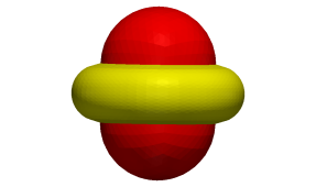
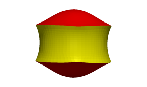
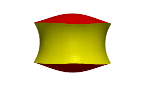
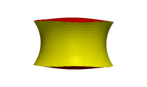
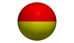
id → s subscript → id 𝑠 \vec{\rm id}_{s} μ → 2 subscript → 𝜇 2 \vec{\mu}_{2} μ → 1 subscript → 𝜇 1 \vec{\mu}_{1} ν → 2 subscript → 𝜈 2 \vec{\nu}_{2} ν → 1 subscript → 𝜈 1 \vec{\nu}_{1} Γ 2 subscript Γ 2 \Gamma_{2} Γ 1 subscript Γ 1 \Gamma_{1} γ 𝛾 \gamma Figure 1. Sketch of Γ = Γ 1 ∪ γ ∪ Γ 2 Γ subscript Γ 1 𝛾 subscript Γ 2 \Gamma=\Gamma_{1}\cup\gamma\cup\Gamma_{2} ν → i subscript → 𝜈 𝑖 \vec{\nu}_{i} μ → i subscript → 𝜇 𝑖 \vec{\mu}_{i} id → s subscript → id 𝑠 \vec{\rm id}_{s} γ 𝛾 \gamma d = 3 𝑑 3 d=3
Throughout this paper we will investigate two different types of junction
conditions on γ ( t ) 𝛾 𝑡 \gamma(t)
C 0 superscript 𝐶 0 C^{0} γ ( t ) = ∂ Γ 1 ( t ) = ∂ Γ 2 ( t ) , 𝛾 𝑡 subscript Γ 1 𝑡 subscript Γ 2 𝑡 \displaystyle\quad\gamma(t)=\partial\Gamma_{1}(t)=\partial\Gamma_{2}(t)\,, (2a)
C 1 superscript 𝐶 1 C^{1} γ ( t ) = ∂ Γ 1 ( t ) = ∂ Γ 2 ( t ) and ν → 1 = ν → 2 on γ ( t ) . formulae-sequence 𝛾 𝑡 subscript Γ 1 𝑡 subscript Γ 2 𝑡 and subscript → 𝜈 1 subscript → 𝜈 2 on 𝛾 𝑡 \displaystyle\quad\gamma(t)=\partial\Gamma_{1}(t)=\partial\Gamma_{2}(t)\ \text{ and }\ \vec{\nu}_{1}=\vec{\nu}_{2}\quad\text{on }\gamma(t)\,. (2b)
Of course, in the case (2b μ → 1 = − μ → 2 subscript → 𝜇 1 subscript → 𝜇 2 \vec{\mu}_{1}=-\vec{\mu}_{2} μ → i subscript → 𝜇 𝑖 \vec{\mu}_{i} Γ i ( t ) subscript Γ 𝑖 𝑡 \Gamma_{i}(t) γ ( t ) 𝛾 𝑡 \gamma(t)
In order to formulate the governing problems in more detail, we
denote by ∇ s = ( ∂ s 1 , … , ∂ s d ) subscript ∇ 𝑠 subscript subscript 𝑠 1 … subscript subscript 𝑠 𝑑 \nabla_{\!s}=(\partial_{s_{1}},\ldots,\partial_{s_{d}}) Γ i subscript Γ 𝑖 \Gamma_{i} ∇ s χ → = ( ∂ s j χ k ) k , j = 1 d subscript ∇ 𝑠 → 𝜒 superscript subscript subscript subscript 𝑠 𝑗 subscript 𝜒 𝑘 𝑘 𝑗
1 𝑑 \nabla_{\!s}\,\vec{\chi}=\left(\partial_{s_{j}}\,\chi_{k}\right)_{k,j=1}^{d} Δ s = ∇ s . ∇ s = ∑ j = 1 d ∂ s j 2 formulae-sequence subscript Δ 𝑠 subscript ∇ 𝑠 subscript ∇ 𝑠 superscript subscript 𝑗 1 𝑑 superscript subscript subscript 𝑠 𝑗 2 \Delta_{s}=\nabla_{\!s}\,.\,\nabla_{\!s}=\sum_{j=1}^{d}\partial_{s_{j}}^{2}
ϰ → i = ϰ i ν → i = Δ s id → on Γ i , formulae-sequence subscript → italic-ϰ 𝑖 subscript italic-ϰ 𝑖 subscript → 𝜈 𝑖 subscript Δ 𝑠 → id on Γ i \vec{\varkappa}_{i}=\varkappa_{i}\,\vec{\nu}_{i}=\Delta_{s}\,\vec{\rm id}\qquad\mbox{on $\Gamma_{i}$}\,, (3)
where id → → id \vec{\rm id} ℝ d superscript ℝ 𝑑 {\mathbb{R}}^{d} ϰ i subscript italic-ϰ 𝑖 \varkappa_{i} Γ i subscript Γ 𝑖 \Gamma_{i} Γ i subscript Γ 𝑖 \Gamma_{i} ϰ i , j subscript italic-ϰ 𝑖 𝑗
\varkappa_{i,j} j = 1 , … , d − 1 𝑗 1 … 𝑑 1
j=1,\ldots,d-1 ν → i subscript → 𝜈 𝑖 \vec{\nu}_{i} d 𝑑 d − ∇ s ν → i : ℝ d → ℝ d : subscript ∇ 𝑠 subscript → 𝜈 𝑖 → superscript ℝ 𝑑 superscript ℝ 𝑑 -\nabla_{\!s}\,\vec{\nu}_{i}:{\mathbb{R}}^{d}\to{\mathbb{R}}^{d} [17 , p. 152] ,
where a different sign convention is used.
The map − ∇ s ν → i subscript ∇ 𝑠 subscript → 𝜈 𝑖 -\nabla_{\!s}\,\vec{\nu}_{i} ϰ i subscript italic-ϰ 𝑖 \varkappa_{i} 𝒦 i subscript 𝒦 𝑖 {\mathcal{K}}_{i} Γ i subscript Γ 𝑖 \Gamma_{i}
ϰ i = ∑ j = 1 d − 1 ϰ i , j = − tr ( ∇ s ν → i ) = − ∇ s . ν → i and 𝒦 i = ∏ j = 1 d − 1 ϰ i , j . formulae-sequence subscript italic-ϰ 𝑖 superscript subscript 𝑗 1 𝑑 1 subscript italic-ϰ 𝑖 𝑗
tr subscript ∇ 𝑠 subscript → 𝜈 𝑖 subscript ∇ 𝑠 subscript → 𝜈 𝑖 and subscript 𝒦 𝑖
superscript subscript product 𝑗 1 𝑑 1 subscript italic-ϰ 𝑖 𝑗
\varkappa_{i}=\sum_{j=1}^{d-1}\varkappa_{i,j}=-\operatorname{tr}(\nabla_{\!s}\,\vec{\nu}_{i})=-\nabla_{\!s}\,.\,\vec{\nu}_{i}\qquad\mbox{and}\qquad{\mathcal{K}}_{i}=\prod_{j=1}^{d-1}\varkappa_{i,j}\,. (4)
Throughout the paper the main case we are interested in is d = 3 𝑑 3 d=3 d = 2 𝑑 2 d=2 1
E ( ( Γ i ( t ) ) i = 1 2 ) = ∑ i = 1 2 [ 1 2 α i ∫ Γ i ( t ) ( ϰ i − ϰ ¯ i ) 2 d ℋ d − 1 + α i G ∫ Γ i ( t ) 𝒦 i d ℋ d − 1 ] + ς ℋ d − 2 ( γ ( t ) ) , 𝐸 superscript subscript subscript Γ 𝑖 𝑡 𝑖 1 2 superscript subscript 𝑖 1 2 delimited-[] 1 2 subscript 𝛼 𝑖 subscript subscript Γ 𝑖 𝑡 superscript subscript italic-ϰ 𝑖 subscript ¯ italic-ϰ 𝑖 2 differential-d superscript ℋ 𝑑 1 subscript superscript 𝛼 𝐺 𝑖 subscript subscript Γ 𝑖 𝑡 subscript 𝒦 𝑖 differential-d superscript ℋ 𝑑 1 𝜍 superscript ℋ 𝑑 2 𝛾 𝑡 E((\Gamma_{i}(t))_{i=1}^{2})=\sum_{i=1}^{2}\left[\tfrac{1}{2}\,\alpha_{i}\,\int_{\Gamma_{i}(t)}(\varkappa_{i}-{\overline{\varkappa}}_{i})^{2}\;{\rm d}{\mathcal{H}}^{d-1}+\alpha^{G}_{i}\,\int_{\Gamma_{i}(t)}{\mathcal{K}}_{i}\;{\rm d}{\mathcal{H}}^{d-1}\right]+\varsigma\,\mathcal{H}^{d-2}(\gamma(t))\,, (5)
where ϰ i subscript italic-ϰ 𝑖 \varkappa_{i} 𝒦 i subscript 𝒦 𝑖 {\mathcal{K}}_{i} Γ i ( t ) subscript Γ 𝑖 𝑡 \Gamma_{i}(t) i = 1 , 2 𝑖 1 2
i=1,2 ς ∈ ℝ ≥ 0 𝜍 subscript ℝ absent 0 \varsigma\in{\mathbb{R}}_{\geq 0} α i ∈ ℝ > 0 subscript 𝛼 𝑖 subscript ℝ absent 0 \alpha_{i}\in{\mathbb{R}}_{>0} α i G ∈ ℝ subscript superscript 𝛼 𝐺 𝑖 ℝ \alpha^{G}_{i}\in{\mathbb{R}} Γ i ( t ) subscript Γ 𝑖 𝑡 \Gamma_{i}(t) i = 1 , 2 𝑖 1 2
i=1,2 ℋ k superscript ℋ 𝑘 \mathcal{H}^{k} k = 0 , 1 , 2 𝑘 0 1 2
k=0,1,2 k 𝑘 k ℝ d superscript ℝ 𝑑 {\mathbb{R}}^{d}
In the case d = 2 𝑑 2 d=2 ς = α 1 G = α 2 G = 0 𝜍 subscript superscript 𝛼 𝐺 1 subscript superscript 𝛼 𝐺 2 0 \varsigma=\alpha^{G}_{1}=\alpha^{G}_{2}=0 d = 3 𝑑 3 d=3
∑ i = 1 2 [ 1 2 α i ∫ Γ i ( t ) ϰ i 2 d ℋ 2 + α i G ∫ Γ i ( t ) 𝒦 i d ℋ 2 ] superscript subscript 𝑖 1 2 delimited-[] 1 2 subscript 𝛼 𝑖 subscript subscript Γ 𝑖 𝑡 subscript superscript italic-ϰ 2 𝑖 differential-d superscript ℋ 2 subscript superscript 𝛼 𝐺 𝑖 subscript subscript Γ 𝑖 𝑡 subscript 𝒦 𝑖 differential-d superscript ℋ 2 \sum_{i=1}^{2}\left[\tfrac{1}{2}\,\alpha_{i}\,\int_{\Gamma_{i}(t)}\varkappa^{2}_{i}\;{\rm d}{\mathcal{H}}^{2}+\alpha^{G}_{i}\,\int_{\Gamma_{i}(t)}{\mathcal{K}}_{i}\;{\rm d}{\mathcal{H}}^{2}\right] (6)
to the energy (5
α i G ∈ [ − 2 α i , 0 ] , i = 1 , 2 . formulae-sequence subscript superscript 𝛼 𝐺 𝑖 2 subscript 𝛼 𝑖 0 𝑖 1 2
\alpha^{G}_{i}\in[-2\,\alpha_{i},0]\,,\quad i=1,2\,. (7)
In the C 1 superscript 𝐶 1 C^{1} 2b ∑ i = 1 2 𝒦 i d ℋ 2 superscript subscript 𝑖 1 2 subscript 𝒦 𝑖 d superscript ℋ 2 \sum_{i=1}^{2}{\mathcal{K}}_{i}\;{\rm d}{\mathcal{H}}^{2} 12 5 α i G ≥ max { α 1 G , α 2 G } − 2 α i subscript superscript 𝛼 𝐺 𝑖 subscript superscript 𝛼 𝐺 1 subscript superscript 𝛼 𝐺 2 2 subscript 𝛼 𝑖 \alpha^{G}_{i}\geq\max\{\alpha^{G}_{1},\alpha^{G}_{2}\}-2\,\alpha_{i} i = 1 , 2 𝑖 1 2
i=1,2
min { α 1 , α 2 } ≥ 1 2 | α 1 G − α 2 G | . subscript 𝛼 1 subscript 𝛼 2 1 2 subscript superscript 𝛼 𝐺 1 subscript superscript 𝛼 𝐺 2 \min\{\alpha_{1},\alpha_{2}\}\geq\tfrac{1}{2}\,|\alpha^{G}_{1}-\alpha^{G}_{2}|\,. (8)
Variational problems for integrals including the energy
(6 [33 , p. 364] , in order to be able to show a priori estimates.
As discussed in [33 ] , the condition of definiteness leads to the
constraints (7 8 5 C 0 superscript 𝐶 0 C^{0} C 1 superscript 𝐶 1 C^{1}
In the case d = 3 𝑑 3 d=3 3
id → s s = ϰ → γ on γ ( t ) , subscript → id 𝑠 𝑠 subscript → italic-ϰ 𝛾 on 𝛾 𝑡
\vec{\rm id}_{ss}=\vec{\varkappa}_{\gamma}\quad\text{on }\ \gamma(t)\,, (9)
where ϰ → γ subscript → italic-ϰ 𝛾 \vec{\varkappa}_{\gamma} γ ( t ) 𝛾 𝑡 \gamma(t) s 𝑠 s γ ( t ) 𝛾 𝑡 \gamma(t)
μ → i = ( − 1 ) i ν → i × id → s on γ ( t ) , subscript → 𝜇 𝑖 superscript 1 𝑖 subscript → 𝜈 𝑖 subscript → id 𝑠 on 𝛾 𝑡
\vec{\mu}_{i}=(-1)^{i}\,\vec{\nu}_{i}\times\vec{\rm id}_{s}\quad\text{on }\ \gamma(t), (10)
for i = 1 , 2 𝑖 1 2
i=1,2 Γ i ( t ) subscript Γ 𝑖 𝑡 \Gamma_{i}(t) γ ( t ) 𝛾 𝑡 \gamma(t) μ → i subscript → 𝜇 𝑖 \vec{\mu}_{i} id → s subscript → id 𝑠 \vec{\rm id}_{s} ∂ Γ i ( t ) subscript Γ 𝑖 𝑡 \partial\Gamma_{i}(t) Γ i ( t ) subscript Γ 𝑖 𝑡 \Gamma_{i}(t) 9
id → s s = ϰ → γ = ( ϰ → γ . μ → i ) μ → i + ( ϰ → γ . ν → i ) ν → i on γ ( t ) , \vec{\rm id}_{ss}=\vec{\varkappa}_{\gamma}=(\vec{\varkappa}_{\gamma}\,.\,\vec{\mu}_{i})\,\vec{\mu}_{i}+(\vec{\varkappa}_{\gamma}\,.\,\vec{\nu}_{i})\,\vec{\nu}_{i}\quad\text{on }\ \gamma(t)\,, (11)
where ϰ → γ . μ → i formulae-sequence subscript → italic-ϰ 𝛾 subscript → 𝜇 𝑖 \vec{\varkappa}_{\gamma}\,.\,\vec{\mu}_{i} ϰ → γ . ν → i formulae-sequence subscript → italic-ϰ 𝛾 subscript → 𝜈 𝑖 \vec{\varkappa}_{\gamma}\,.\,\vec{\nu}_{i} γ ( t ) 𝛾 𝑡 \gamma(t) Γ i ( t ) subscript Γ 𝑖 𝑡 \Gamma_{i}(t) i = 1 , 2 𝑖 1 2
i=1,2
∫ Γ i ( t ) 𝒦 i d ℋ 2 = 2 π m ( Γ i ( t ) ) + ∫ γ ( t ) ϰ → γ . μ → i d ℋ 1 , formulae-sequence subscript subscript Γ 𝑖 𝑡 subscript 𝒦 𝑖 differential-d superscript ℋ 2 2 𝜋 𝑚 subscript Γ 𝑖 𝑡 subscript 𝛾 𝑡 subscript → italic-ϰ 𝛾 subscript → 𝜇 𝑖 d superscript ℋ 1 \int_{\Gamma_{i}(t)}{\mathcal{K}}_{i}\;{\rm d}{\mathcal{H}}^{2}=2\,\pi\,m(\Gamma_{i}(t))+\int_{\gamma(t)}\vec{\varkappa}_{\gamma}\,.\,\vec{\mu}_{i}\;{\rm d}{\mathcal{H}}^{1}, (12)
where m ( Γ i ( t ) ) ∈ ℤ 𝑚 subscript Γ 𝑖 𝑡 ℤ m(\Gamma_{i}(t))\in\mathbb{Z} Γ i ( t ) subscript Γ 𝑖 𝑡 \Gamma_{i}(t) 5
E ( ( Γ i ( t ) ) i = 1 2 ) = 𝐸 superscript subscript subscript Γ 𝑖 𝑡 𝑖 1 2 absent \displaystyle E((\Gamma_{i}(t))_{i=1}^{2})=
∑ i = 1 2 [ 1 2 α i ∫ Γ i ( t ) ( ϰ i − ϰ ¯ i ) 2 d ℋ 2 + α i G [ ∫ γ ( t ) ϰ → γ . μ → i d ℋ 1 + 2 π m ( Γ i ( t ) ) ] ] + ς ℋ 1 ( γ ( t ) ) . \displaystyle\quad\sum_{i=1}^{2}\left[\tfrac{1}{2}\,\alpha_{i}\,\int_{\Gamma_{i}(t)}(\varkappa_{i}-{\overline{\varkappa}}_{i})^{2}\;{\rm d}{\mathcal{H}}^{2}+\alpha^{G}_{i}\left[\int_{\gamma(t)}\vec{\varkappa}_{\gamma}\,.\,\vec{\mu}_{i}\;{\rm d}{\mathcal{H}}^{1}+2\,\pi\,m(\Gamma_{i}(t))\right]\right]+\varsigma\,\mathcal{H}^{1}(\gamma(t))\,. (13)
We note that we use a sign for the conormal that is different from many
authors in differential geometry, and hence we obtain a different sign in
the Gauss–Bonnet formula.
In some cases, in particular in applications for biomembranes, cf. [38 ] , the surface areas of Γ 1 ( t ) subscript Γ 1 𝑡 \Gamma_{1}(t) Γ 2 ( t ) subscript Γ 2 𝑡 \Gamma_{2}(t) Γ ( t ) Γ 𝑡 \Gamma(t) d = 2 𝑑 2 d=2
E λ ( ( Γ i ( t ) ) i = 1 2 ) = E ( ( Γ i ( t ) ) i = 1 2 ) + λ V ( t ) ℒ d ( Ω ( t ) ) + ∑ i = 1 2 λ i A ( t ) ℋ d − 1 ( Γ i ( t ) ) , subscript 𝐸 𝜆 superscript subscript subscript Γ 𝑖 𝑡 𝑖 1 2 𝐸 superscript subscript subscript Γ 𝑖 𝑡 𝑖 1 2 superscript 𝜆 𝑉 𝑡 superscript ℒ 𝑑 Ω 𝑡 superscript subscript 𝑖 1 2 subscript superscript 𝜆 𝐴 𝑖 𝑡 superscript ℋ 𝑑 1 subscript Γ 𝑖 𝑡 E_{\lambda}((\Gamma_{i}(t))_{i=1}^{2})=E((\Gamma_{i}(t))_{i=1}^{2})+\lambda^{V}(t)\,\mathcal{L}^{d}(\Omega(t))+\sum_{i=1}^{2}\lambda^{A}_{i}(t)\,\mathcal{H}^{d-1}(\Gamma_{i}(t))\,, (14)
where Ω ( t ) Ω 𝑡 \Omega(t) Γ ( t ) Γ 𝑡 \Gamma(t) ℒ d superscript ℒ 𝑑 \mathcal{L}^{d} ℝ d superscript ℝ 𝑑 \mathbb{R}^{d} λ i A ( t ) subscript superscript 𝜆 𝐴 𝑖 𝑡 \lambda^{A}_{i}(t) λ V ( t ) superscript 𝜆 𝑉 𝑡 \lambda^{V}(t)
For the convenience of the reader,
we end this section by stating the strong formulations of the
L 2 superscript 𝐿 2 L^{2} 5 2a 2b 3
The weighted L 2 superscript 𝐿 2 L^{2} 2 2 d = 2 𝑑 2 d=2 d = 3 𝑑 3 d=3
𝒱 → . ν → i = − α i Δ s ϰ i + 1 2 α i ( ϰ i − ϰ ¯ i ) 2 ϰ i − α i ( ϰ i − ϰ ¯ i ) | ∇ s ν → i | 2 on Γ i ( t ) , i = 1 , 2 . formulae-sequence → 𝒱 formulae-sequence subscript → 𝜈 𝑖 subscript 𝛼 𝑖 subscript Δ 𝑠 subscript italic-ϰ 𝑖 1 2 subscript 𝛼 𝑖 superscript subscript italic-ϰ 𝑖 subscript ¯ italic-ϰ 𝑖 2 subscript italic-ϰ 𝑖 subscript 𝛼 𝑖 subscript italic-ϰ 𝑖 subscript ¯ italic-ϰ 𝑖 superscript subscript ∇ 𝑠 subscript → 𝜈 𝑖 2 on subscript Γ 𝑖 𝑡
𝑖 1 2
\vec{\mathcal{V}}\,.\,\vec{\nu}_{i}=-\alpha_{i}\,\Delta_{s}\,\varkappa_{i}+\tfrac{1}{2}\,\alpha_{i}\,(\varkappa_{i}-{\overline{\varkappa}}_{i})^{2}\,\varkappa_{i}-\alpha_{i}\,(\varkappa_{i}-{\overline{\varkappa}}_{i})\,|\nabla_{\!s}\,\vec{\nu}_{i}|^{2}\quad\text{on }\Gamma_{i}(t)\,,\ i=1,2\,. (15)
See (8 15 14 15
𝒱 → . ν → i = − α i Δ s ϰ i + 1 2 α i ( ϰ i − ϰ ¯ i ) 2 ϰ i − α i ( ϰ i − ϰ ¯ i ) | ∇ s ν → i | 2 + λ i A ϰ i − λ V on Γ i ( t ) , formulae-sequence → 𝒱 subscript → 𝜈 𝑖 subscript 𝛼 𝑖 subscript Δ 𝑠 subscript italic-ϰ 𝑖 1 2 subscript 𝛼 𝑖 superscript subscript italic-ϰ 𝑖 subscript ¯ italic-ϰ 𝑖 2 subscript italic-ϰ 𝑖 subscript 𝛼 𝑖 subscript italic-ϰ 𝑖 subscript ¯ italic-ϰ 𝑖 superscript subscript ∇ 𝑠 subscript → 𝜈 𝑖 2 subscript superscript 𝜆 𝐴 𝑖 subscript italic-ϰ 𝑖 superscript 𝜆 𝑉 on subscript Γ 𝑖 𝑡
\vec{\mathcal{V}}\,.\,\vec{\nu}_{i}=-\alpha_{i}\,\Delta_{s}\,\varkappa_{i}+\tfrac{1}{2}\,\alpha_{i}\,(\varkappa_{i}-{\overline{\varkappa}}_{i})^{2}\,\varkappa_{i}-\alpha_{i}\,(\varkappa_{i}-{\overline{\varkappa}}_{i})\,|\nabla_{\!s}\,\vec{\nu}_{i}|^{2}+\lambda^{A}_{i}\,\varkappa_{i}-\lambda^{V}\quad\text{on }\Gamma_{i}(t)\,, (16)
for i = 1 , 2 𝑖 1 2
i=1,2 13
In the case d = 3 𝑑 3 d=3 I I i I subscript I 𝑖 {\rm I\!I}_{i} Γ i ( t ) subscript Γ 𝑖 𝑡 \Gamma_{i}(t)
I I i ( 𝔱 → 1 , 𝔱 → 2 ) = − [ ∂ 𝔱 → 1 ν → i ] . 𝔱 → 2 = − [ ( ∇ s ν → i ) 𝔱 → 1 ] . 𝔱 → 2 on Γ i ( t ) , formulae-sequence I subscript I 𝑖 subscript → 𝔱 1 subscript → 𝔱 2 delimited-[] subscript subscript → 𝔱 1 subscript → 𝜈 𝑖 subscript → 𝔱 2 delimited-[] subscript ∇ 𝑠 subscript → 𝜈 𝑖 subscript → 𝔱 1 subscript → 𝔱 2 on subscript Γ 𝑖 𝑡
{\rm I\!I}_{i}(\vec{\mathfrak{t}}_{1},\vec{\mathfrak{t}}_{2})=-[\partial_{\vec{\mathfrak{t}}_{1}}\,\vec{\nu}_{i}]\,.\,\vec{\mathfrak{t}}_{2}=-[(\nabla_{\!s}\,\vec{\nu}_{i})\,\vec{\mathfrak{t}}_{1}]\,.\,\vec{\mathfrak{t}}_{2}\qquad\text{on }\ \Gamma_{i}(t)\,, (17)
for all tangential vectors 𝔱 → j subscript → 𝔱 𝑗 \vec{\mathfrak{t}}_{j} j = 1 , 2 𝑗 1 2
j=1,2 I I i ( ⋅ , ⋅ ) I subscript I 𝑖 ⋅ ⋅ {\rm I\!I}_{i}(\cdot,\cdot) ∇ s ν → i subscript ∇ 𝑠 subscript → 𝜈 𝑖 \nabla_{\!s}\,\vec{\nu}_{i}
τ i = I I i ( id → s , μ → i ) on γ ( t ) , subscript 𝜏 𝑖 I subscript I 𝑖 subscript → id 𝑠 subscript → 𝜇 𝑖 on 𝛾 𝑡
\tau_{i}={\rm I\!I}_{i}(\vec{\rm id}_{s},\vec{\mu}_{i})\qquad\text{on }\gamma(t)\,, (18)
i.e. τ i = − ( ν → i ) s . μ → i formulae-sequence subscript 𝜏 𝑖 subscript subscript → 𝜈 𝑖 𝑠 subscript → 𝜇 𝑖 \tau_{i}=-(\vec{\nu}_{i})_{s}\,.\,\vec{\mu}_{i} γ ( t ) 𝛾 𝑡 \gamma(t)
Still considering the case d = 3 𝑑 3 d=3 C 0 superscript 𝐶 0 C^{0} γ ( t ) 𝛾 𝑡 \gamma(t)
α i ( ϰ i − ϰ ¯ i ) + α i G ϰ → γ . ν → i = 0 on γ ( t ) , i = 1 , 2 , formulae-sequence subscript 𝛼 𝑖 subscript italic-ϰ 𝑖 subscript ¯ italic-ϰ 𝑖 subscript superscript 𝛼 𝐺 𝑖 subscript → italic-ϰ 𝛾 formulae-sequence subscript → 𝜈 𝑖 0 on 𝛾 𝑡
𝑖 1 2
\displaystyle\alpha_{i}\,(\varkappa_{i}-{\overline{\varkappa}}_{i})+\alpha^{G}_{i}\,\vec{\varkappa}_{\gamma}\,.\,\vec{\nu}_{i}=0\quad\text{on }\ \gamma(t)\,,\quad i=1,2\,, (19a)
∑ i = 1 2 [ ( ( α i ( ∇ s ϰ i ) . μ → i − α i G ( τ i ) s ) ν → i − ( 1 2 α i ( ϰ i − ϰ ¯ i ) 2 + α i G 𝒦 i + λ i A ) μ → i ] + ς ϰ → γ = ϱ 𝒱 → on γ ( t ) , \displaystyle\sum_{i=1}^{2}\left[((\alpha_{i}\,(\nabla_{\!s}\,\varkappa_{i})\,.\,\vec{\mu}_{i}-\alpha^{G}_{i}\,(\tau_{i})_{s})\,\vec{\nu}_{i}-(\tfrac{1}{2}\,\alpha_{i}\,(\varkappa_{i}-{\overline{\varkappa}}_{i})^{2}+\alpha^{G}_{i}\,{\mathcal{K}}_{i}+\lambda^{A}_{i})\,\vec{\mu}_{i}\right]+\varsigma\,\vec{\varkappa}_{\gamma}=\varrho\,\vec{\mathcal{V}}\quad\text{on }\ \gamma(t)\,, (19b)
see (12a 14 19a 19b μ → i subscript → 𝜇 𝑖 \vec{\mu}_{i} ν → i subscript → 𝜈 𝑖 \vec{\nu}_{i} ϰ → γ subscript → italic-ϰ 𝛾 \vec{\varkappa}_{\gamma} γ ( t ) 𝛾 𝑡 \gamma(t) Γ 1 subscript Γ 1 \Gamma_{1} Γ 2 subscript Γ 2 \Gamma_{2} C 0 superscript 𝐶 0 C^{0} [6 ] .
In the C 1 superscript 𝐶 1 C^{1} ν → = ν → 1 = ν → 2 → 𝜈 subscript → 𝜈 1 subscript → 𝜈 2 \vec{\nu}=\vec{\nu}_{1}=\vec{\nu}_{2} μ → = μ → 2 = − μ → 1 → 𝜇 subscript → 𝜇 2 subscript → 𝜇 1 \vec{\mu}=\vec{\mu}_{2}=-\vec{\mu}_{1} γ ( t ) 𝛾 𝑡 \gamma(t) γ ( t ) 𝛾 𝑡 \gamma(t) 2 E 𝐸 E E λ subscript 𝐸 𝜆 E_{\lambda}
[ α i ( ϰ i − ϰ ¯ i ) ] 1 2 + [ α i G ] 1 2 ϰ → γ . ν → = 0 on γ ( t ) , formulae-sequence superscript subscript delimited-[] subscript 𝛼 𝑖 subscript italic-ϰ 𝑖 subscript ¯ italic-ϰ 𝑖 1 2 superscript subscript delimited-[] subscript superscript 𝛼 𝐺 𝑖 1 2 subscript → italic-ϰ 𝛾 → 𝜈 0 on 𝛾 𝑡
\displaystyle[\alpha_{i}\,(\varkappa_{i}-{\overline{\varkappa}}_{i})]_{1}^{2}+[\alpha^{G}_{i}]_{1}^{2}\,\vec{\varkappa}_{\gamma}\,.\,\vec{\nu}=0\quad\text{on }\ \gamma(t)\,, (20a)
[ α i ( ∇ s ϰ i ) ] 1 2 . μ → + ς ϰ → γ . ν → − [ α i G ] 1 2 τ s = ϱ 𝒱 → . ν → on γ ( t ) , formulae-sequence superscript subscript delimited-[] subscript 𝛼 𝑖 subscript ∇ 𝑠 subscript italic-ϰ 𝑖 1 2 → 𝜇 𝜍 subscript → italic-ϰ 𝛾 → 𝜈 superscript subscript delimited-[] subscript superscript 𝛼 𝐺 𝑖 1 2 subscript 𝜏 𝑠 italic-ϱ → 𝒱 → 𝜈 on 𝛾 𝑡
\displaystyle[\alpha_{i}\,(\nabla_{\!s}\,\varkappa_{i})]_{1}^{2}\,.\,\vec{\mu}+\varsigma\,\vec{\varkappa}_{\gamma}\,.\,\vec{\nu}-[\alpha^{G}_{i}]_{1}^{2}\,\tau_{s}=\varrho\,\vec{\mathcal{V}}\,.\,\vec{\nu}\quad\text{on }\ \gamma(t)\,, (20b)
[ − 1 2 α i ( ϰ i − ϰ ¯ i ) 2 + α i ( ϰ i − ϰ ¯ i ) ( ϰ i − ϰ → γ . ν → ) − λ i A ] 1 2 + [ α i G ] 1 2 τ 2 + ς ϰ → γ . μ → = ϱ 𝒱 → . μ → on γ ( t ) , \displaystyle[-\tfrac{1}{2}\,\alpha_{i}\,(\varkappa_{i}-{\overline{\varkappa}}_{i})^{2}+\alpha_{i}\,(\varkappa_{i}-{\overline{\varkappa}}_{i})\,(\varkappa_{i}-\vec{\varkappa}_{\gamma}\,.\,\vec{\nu})-\lambda^{A}_{i}]_{1}^{2}+[\alpha^{G}_{i}]_{1}^{2}\,\tau^{2}+\varsigma\,\vec{\varkappa}_{\gamma}\,.\,\vec{\mu}=\varrho\,\vec{\mathcal{V}}\,.\,\vec{\mu}\quad\text{on }\ \gamma(t)\,, (20c)
where τ = τ 2 = − τ 1 𝜏 subscript 𝜏 2 subscript 𝜏 1 \tau=\tau_{2}=-\tau_{1} γ ( t ) 𝛾 𝑡 \gamma(t) Γ ( t ) Γ 𝑡 \Gamma(t) 20a ϱ = 0 italic-ϱ 0 \varrho=0 [23 ] , see also [24 , (2.7b,a,c)] .
In terms of counting the number of equations, we see that (20a ν → 1 = ν → 2 subscript → 𝜈 1 subscript → 𝜈 2 \vec{\nu}_{1}=\vec{\nu}_{2} 15a 24a 20a
3. Weak formulation
In this section we derive a weak formulation of a generalized L 2 superscript 𝐿 2 L^{2} E ( ( Γ i ( t ) ) i = 1 2 ) 𝐸 superscript subscript subscript Γ 𝑖 𝑡 𝑖 1 2 E((\Gamma_{i}(t))_{i=1}^{2}) L 2 superscript 𝐿 2 L^{2} 29 ϱ = 0 italic-ϱ 0 \varrho=0 f Γ subscript 𝑓 Γ f_{\Gamma} E ( ( Γ i ( t ) ) i = 1 2 ) 𝐸 superscript subscript subscript Γ 𝑖 𝑡 𝑖 1 2 E((\Gamma_{i}(t))_{i=1}^{2}) 28a f Γ subscript 𝑓 Γ f_{\Gamma} 4
On recalling (1 x → ( ⋅ , t ) → 𝑥 ⋅ 𝑡 \vec{x}(\cdot,t) Γ ( t ) Γ 𝑡 \Gamma(t)
( ∂ t ∘ ϕ ) ∣ Γ i ( t ) = ( ϕ t + 𝒱 → . ∇ ϕ ) ∣ Γ i ( t ) ∀ ϕ ∈ H 1 ( Γ i , T ) , (\partial_{t}^{\circ}\,\phi)\!\mid_{\Gamma_{i}(t)}=(\phi_{t}+\vec{\mathcal{V}}\,.\,\nabla\,\phi)\!\mid_{\Gamma_{i}(t)}\qquad\forall\ \phi\in H^{1}({\Gamma_{i,T}})\,, (1)
where we have defined the space-time surfaces
Γ i , T := ⋃ t ∈ [ 0 , T ] Γ i ( t ) × { t } , i = 1 , 2 , and Γ T := ⋃ t ∈ [ 0 , T ] Γ ( t ) × { t } . formulae-sequence assign subscript Γ 𝑖 𝑇
subscript 𝑡 0 𝑇 subscript Γ 𝑖 𝑡 𝑡 formulae-sequence 𝑖 1 2 and
assign subscript Γ 𝑇 subscript 𝑡 0 𝑇 Γ 𝑡 𝑡 {\Gamma_{i,T}}:=\bigcup_{t\in[0,T]}\Gamma_{i}(t)\times\{t\}\,,\ i=1,2\,,\quad\text{and}\quad{\Gamma_{T}}:=\bigcup_{t\in[0,T]}\Gamma(t)\times\{t\}\,.
Here we stress that (1 ϕ t subscript italic-ϕ 𝑡 \phi_{t} ∇ ϕ ∇ italic-ϕ \nabla\,\phi ϕ ∈ H 1 ( Γ i , T ) italic-ϕ superscript 𝐻 1 subscript Γ 𝑖 𝑇
\phi\in H^{1}({\Gamma_{i,T}})
d d t ⟨ ψ i , ϕ i ⟩ Γ i ( t ) = ⟨ ∂ t ∘ ψ i , ϕ ⟩ Γ i ( t ) + ⟨ ψ i , ∂ t ∘ ϕ i ⟩ Γ i ( t ) + ⟨ ψ i ϕ i , ∇ s . 𝒱 → ⟩ Γ i ( t ) ∀ ψ i , ϕ i ∈ H 1 ( Γ i , T ) , \frac{\rm d}{{\rm d}t}\left\langle\psi_{i},\phi_{i}\right\rangle_{\Gamma_{i}(t)}=\left\langle\partial_{t}^{\circ}\,\psi_{i},\phi\right\rangle_{\Gamma_{i}(t)}+\left\langle\psi_{i},\partial_{t}^{\circ}\,\phi_{i}\right\rangle_{\Gamma_{i}(t)}+\left\langle\psi_{i}\,\phi_{i},\nabla_{\!s}\,.\,\vec{\mathcal{V}}\right\rangle_{\Gamma_{i}(t)}\qquad\forall\ \psi_{i},\phi_{i}\in H^{1}({\Gamma_{i,T}})\,, (2)
see Lemma 5.2 in [21 ] .
Here ⟨ ⋅ , ⋅ ⟩ Γ i ( t ) subscript ⋅ ⋅
subscript Γ 𝑖 𝑡 \langle\cdot,\cdot\rangle_{\Gamma_{i}(t)} L 2 superscript 𝐿 2 L^{2} Γ i ( t ) subscript Γ 𝑖 𝑡 \Gamma_{i}(t) ⟨ ⋅ , ⋅ ⟩ Γ ( t ) = ∑ i = 1 2 subscript ⋅ ⋅
Γ 𝑡 superscript subscript 𝑖 1 2 \langle\cdot,\cdot\rangle_{\Gamma(t)}=\sum_{i=1}^{2} ⟨ ⋅ , ⋅ ⟩ Γ i ( t ) subscript ⋅ ⋅
subscript Γ 𝑖 𝑡 \langle\cdot,\cdot\rangle_{\Gamma_{i}(t)} 2
d d t ℋ d − 1 ( Γ i ( t ) ) = ⟨ ∇ s . 𝒱 → , 1 ⟩ Γ i ( t ) = ⟨ ∇ s id → , ∇ s 𝒱 → ⟩ Γ i ( t ) . \frac{\rm d}{{\rm d}t}\,\mathcal{H}^{d-1}(\Gamma_{i}(t))=\left\langle\nabla_{\!s}\,.\,\vec{\mathcal{V}},1\right\rangle_{\Gamma_{i}(t)}=\left\langle\nabla_{\!s}\,\vec{\rm id},\nabla_{\!s}\,\vec{\mathcal{V}}\right\rangle_{\Gamma_{i}(t)}. (3)
Moreover, on recalling Lemma 2.1 from [17 ] , it holds that
d d t ℒ d ( Ω ( t ) ) = ∑ i = 1 2 ⟨ 𝒱 → , ν → i ⟩ Γ i ( t ) . d d 𝑡 superscript ℒ 𝑑 Ω 𝑡 superscript subscript 𝑖 1 2 subscript → 𝒱 subscript → 𝜈 𝑖
subscript Γ 𝑖 𝑡 \frac{\rm d}{{\rm d}t}\,\mathcal{L}^{d}(\Omega(t))=\sum_{i=1}^{2}\left\langle\vec{\mathcal{V}},\vec{\nu}_{i}\right\rangle_{\Gamma_{i}(t)}. (4)
In this section we would like to derive a weak formulation for the
L 2 superscript 𝐿 2 L^{2} E ( ( Γ i ( t ) ) i = 1 2 ) 𝐸 superscript subscript subscript Γ 𝑖 𝑡 𝑖 1 2 E((\Gamma_{i}(t))_{i=1}^{2}) Γ ( t ) = x → ( Υ , t ) Γ 𝑡 → 𝑥 Υ 𝑡 \Gamma(t)=\vec{x}(\Upsilon,t)
H γ 1 ( Γ ( t ) ) := { η ∈ L 2 ( Γ ( t ) ) : \displaystyle H^{1}_{\gamma}(\Gamma(t)):=\{\eta\in L^{2}(\Gamma(t)): η ∣ Γ i ( t ) ∈ H 1 ( Γ i ( t ) ) , i = 1 , 2 , formulae-sequence evaluated-at 𝜂 subscript Γ 𝑖 𝑡 superscript 𝐻 1 subscript Γ 𝑖 𝑡 𝑖 1 2
\displaystyle\ \eta\!\mid_{\Gamma_{i}(t)}\in H^{1}(\Gamma_{i}(t)),i=1,2\,,\
( η ∣ Γ 1 ( t ) ) ∣ γ ( t ) = ( η ∣ Γ 2 ( t ) ) ∣ γ ( t ) = : η ∣ γ ( t ) ∈ H 1 ( γ ( t ) ) } . \displaystyle(\eta\!\mid_{\Gamma_{1}(t)})\!\mid_{\gamma(t)}=(\eta\!\mid_{\Gamma_{2}(t)})\!\mid_{\gamma(t)}=:\eta\!\mid_{\gamma(t)}\in H^{1}(\gamma(t))\}\,.
In addition, for any given χ → ∈ [ H γ 1 ( Γ ( t ) ) ] d → 𝜒 superscript delimited-[] subscript superscript 𝐻 1 𝛾 Γ 𝑡 𝑑 \vec{\chi}\in[H^{1}_{\gamma}(\Gamma(t))]^{d} ε ∈ ( 0 , ε 0 ) 𝜀 0 subscript 𝜀 0 \varepsilon\in(0,\varepsilon_{0}) ε 0 ∈ ℝ > 0 subscript 𝜀 0 subscript ℝ absent 0 \varepsilon_{0}\in{\mathbb{R}}_{>0}
Γ ε ( t ) := { Ψ → ( z → , ε ) : z → ∈ Γ ( t ) } , where Ψ → ( z → , 0 ) = z → and ∂ Ψ → ∂ ε ( z → , 0 ) = χ → ( z → ) ∀ z → ∈ Γ ( t ) . formulae-sequence formulae-sequence assign subscript Γ 𝜀 𝑡 conditional-set → Ψ → 𝑧 𝜀 → 𝑧 Γ 𝑡 where → Ψ → 𝑧 0 → 𝑧 and → Ψ 𝜀 → 𝑧 0 → 𝜒 → 𝑧 for-all → 𝑧 Γ 𝑡 \Gamma_{\varepsilon}(t):=\{\vec{\Psi}(\vec{z},\varepsilon):\vec{z}\in\Gamma(t)\}\,,\ \text{~{}where~{}}\ \vec{\Psi}(\vec{z},0)=\vec{z}\text{~{}and~{}}\tfrac{\partial\vec{\Psi}}{\partial\varepsilon}(\vec{z},0)=\vec{\chi}(\vec{z})\quad\forall\ \vec{z}\in\Gamma(t)\,. (5)
Of course, we have that
Γ ε ( t ) = Γ 1 , ε ( t ) ∪ γ ε ( t ) ∪ Γ 2 , ε ( t ) subscript Γ 𝜀 𝑡 subscript Γ 1 𝜀
𝑡 subscript 𝛾 𝜀 𝑡 subscript Γ 2 𝜀
𝑡 \Gamma_{\varepsilon}(t)=\Gamma_{1,\varepsilon}(t)\cup\gamma_{\varepsilon}(t)\cup\Gamma_{2,\varepsilon}(t)
Γ i , ε ( t ) := { Ψ → ( z → , ε ) : z → ∈ Γ i ( t ) } , i = 1 , 2 , and γ ε ( t ) = ∂ Γ 1 , ε ( t ) = ∂ Γ 2 , ε ( t ) . formulae-sequence assign subscript Γ 𝑖 𝜀
𝑡 conditional-set → Ψ → 𝑧 𝜀 → 𝑧 subscript Γ 𝑖 𝑡 formulae-sequence 𝑖 1 2 and
subscript 𝛾 𝜀 𝑡 subscript Γ 1 𝜀
𝑡 subscript Γ 2 𝜀
𝑡 \Gamma_{i,\varepsilon}(t):=\{\vec{\Psi}(\vec{z},\varepsilon):\vec{z}\in\Gamma_{i}(t)\}\,,\ i=1,2\,,\quad\text{and}\quad\gamma_{\varepsilon}(t)=\partial\Gamma_{1,\varepsilon}(t)=\partial\Gamma_{2,\varepsilon}(t)\,.
Similarly to (3 ℋ d − 1 ( Γ i ( t ) ) superscript ℋ 𝑑 1 subscript Γ 𝑖 𝑡 \mathcal{H}^{d-1}(\Gamma_{i}(t)) Γ ( t ) Γ 𝑡 \Gamma(t) χ → ∈ [ H γ 1 ( Γ ( t ) ) ] d → 𝜒 superscript delimited-[] subscript superscript 𝐻 1 𝛾 Γ 𝑡 𝑑 \vec{\chi}\in[H^{1}_{\gamma}(\Gamma(t))]^{d}
[ δ δ Γ ℋ d − 1 ( Γ i ( t ) ) ] ( χ → ) delimited-[] 𝛿 𝛿 Γ superscript ℋ 𝑑 1 subscript Γ 𝑖 𝑡 → 𝜒 \displaystyle\left[\frac{\delta}{{\delta}\Gamma}\,\mathcal{H}^{d-1}(\Gamma_{i}(t))\right](\vec{\chi}) = d d ε ℋ d − 1 ( Γ i , ε ( t ) ) ∣ ε = 0 absent evaluated-at d d 𝜀 superscript ℋ 𝑑 1 subscript Γ 𝑖 𝜀
𝑡 𝜀 0 \displaystyle=\frac{\rm d}{{\rm d}\varepsilon}\,\mathcal{H}^{d-1}(\Gamma_{i,\varepsilon}(t))\mid_{\varepsilon=0}
= lim ε → 0 1 ε [ ℋ d − 1 ( Γ i , ε ( t ) ) − ℋ d − 1 ( Γ i ( t ) ) ] = ⟨ ∇ s id → , ∇ s χ → ⟩ Γ i ( t ) , absent subscript → 𝜀 0 1 𝜀 delimited-[] superscript ℋ 𝑑 1 subscript Γ 𝑖 𝜀
𝑡 superscript ℋ 𝑑 1 subscript Γ 𝑖 𝑡 subscript subscript ∇ 𝑠 → id subscript ∇ 𝑠 → 𝜒
subscript Γ 𝑖 𝑡 \displaystyle=\lim_{\varepsilon\to 0}\tfrac{1}{\varepsilon}\left[\mathcal{H}^{d-1}(\Gamma_{i,\varepsilon}(t))-\mathcal{H}^{d-1}(\Gamma_{i}(t))\right]=\left\langle\nabla_{\!s}\,\vec{\rm id},\nabla_{\!s}\,\vec{\chi}\right\rangle_{\Gamma_{i}(t)}, (6)
see e.g. the proof of Lemma 1 in [20 ] .
In order to derive a suitable weak formulation, we formally consider
the first variation of (5 3
⟨ Q ¯ ¯ i , θ ϰ → i ⋆ , η → ⟩ Γ i ( t ) + ⟨ ∇ s id → , ∇ s η → ⟩ Γ i ( t ) = ⟨ m → i , η → ⟩ γ ( t ) ∀ η → ∈ [ H 1 ( Γ i ( t ) ) ] d , i = 1 , 2 , formulae-sequence subscript ¯ ¯ 𝑄 subscript 𝑖 𝜃
→ italic-ϰ subscript superscript ⋆ 𝑖 → 𝜂
subscript Γ 𝑖 𝑡 subscript subscript ∇ 𝑠 → id subscript ∇ 𝑠 → 𝜂
subscript Γ 𝑖 𝑡 subscript subscript → m 𝑖 → 𝜂
𝛾 𝑡 formulae-sequence for-all → 𝜂 superscript delimited-[] superscript 𝐻 1 subscript Γ 𝑖 𝑡 𝑑 𝑖 1 2
\left\langle\underline{\underline{Q}}\rule{0.0pt}{0.0pt}_{i,\theta}\,\vec{\varkappa}\rule{0.0pt}{0.0pt}^{\star}_{i},\vec{\eta}\right\rangle_{\Gamma_{i}(t)}+\left\langle\nabla_{\!s}\,\vec{\rm id},\nabla_{\!s}\,\vec{\eta}\right\rangle_{\Gamma_{i}(t)}=\left\langle\vec{\rm m}_{i},\vec{\eta}\right\rangle_{\gamma(t)}\qquad\forall\ \vec{\eta}\in[H^{1}(\Gamma_{i}(t))]^{d}\,,\ i=1,2\,, (7)
where θ ∈ [ 0 , 1 ] 𝜃 0 1 \theta\in[0,1] Q ¯ ¯ i , θ ¯ ¯ 𝑄 subscript 𝑖 𝜃
\underline{\underline{Q}}\rule{0.0pt}{0.0pt}_{i,\theta}
Q ¯ ¯ i , θ = θ Id ¯ ¯ + ( 1 − θ ) ν → i ⊗ ν → i on Γ i ( t ) . ¯ ¯ 𝑄 subscript 𝑖 𝜃
𝜃 ¯ ¯ Id tensor-product 1 𝜃 subscript → 𝜈 𝑖 subscript → 𝜈 𝑖 on subscript Γ 𝑖 𝑡
\underline{\underline{Q}}\rule{0.0pt}{0.0pt}_{i,\theta}=\theta\,\underline{\underline{{\rm Id}}}\rule{0.0pt}{0.0pt}+(1-\theta)\,\vec{\nu}_{i}\otimes\vec{\nu}_{i}\quad\text{on }\ \Gamma_{i}(t)\,. (8)
Of course, (7 ϰ → i ⋆ = ϰ → i → italic-ϰ subscript superscript ⋆ 𝑖 subscript → italic-ϰ 𝑖 \vec{\varkappa}\rule{0.0pt}{0.0pt}^{\star}_{i}=\vec{\varkappa}_{i} m → i subscript → m 𝑖 \vec{\rm m}_{i} μ → i subscript → 𝜇 𝑖 \vec{\mu}_{i} θ ∈ [ 0 , 1 ] 𝜃 0 1 \theta\in[0,1] 3 7 θ = 1 𝜃 1 \theta=1 [10 ] , we also allow θ ∈ [ 0 , 1 ) 𝜃 0 1 \theta\in[0,1) θ = 0 𝜃 0 \theta=0 θ = 0 𝜃 0 \theta=0 θ ∈ [ 0 , 1 ] 𝜃 0 1 \theta\in[0,1]
Similarly to (7 9
⟨ ϰ → γ ⋆ , η → ⟩ γ ( t ) + ⟨ id → s , η → s ⟩ γ ( t ) = 0 ∀ η → ∈ [ H 1 ( γ ( t ) ) ] d . formulae-sequence subscript → italic-ϰ subscript superscript ⋆ 𝛾 → 𝜂
𝛾 𝑡 subscript subscript → id 𝑠 subscript → 𝜂 𝑠
𝛾 𝑡 0 for-all → 𝜂 superscript delimited-[] superscript 𝐻 1 𝛾 𝑡 𝑑 \left\langle\vec{\varkappa}\rule{0.0pt}{0.0pt}^{\star}_{\gamma},\vec{\eta}\right\rangle_{\gamma(t)}+\left\langle\vec{\rm id}_{s},\vec{\eta}_{s}\right\rangle_{\gamma(t)}=0\quad\forall\ \vec{\eta}\in[H^{1}(\gamma(t))]^{d}\,. (9)
Finally, in order to model a C 0 superscript 𝐶 0 C^{0} C 1 superscript 𝐶 1 C^{1}
C 1 ( m → 1 + m → 2 ) = 0 → on γ ( t ) , subscript 𝐶 1 subscript → m 1 subscript → m 2 → 0 on 𝛾 𝑡
C_{1}\,(\vec{\rm m}_{1}+\vec{\rm m}_{2})=\vec{0}\qquad\text{on}\quad\gamma(t)\,, (10)
where C 1 = 0 subscript 𝐶 1 0 C_{1}=0 C 0 superscript 𝐶 0 C^{0} C 1 = 1 subscript 𝐶 1 1 C_{1}=1 C 1 superscript 𝐶 1 C^{1}
We now define the Lagrangian
L ( ( Γ i ( t ) , ϰ → i ⋆ , m → i , y → i ) i = 1 2 , ϰ → γ ⋆ , z → , ϕ → ) = ∑ i = 1 2 [ 1 2 α i ⟨ ϰ → i ⋆ − ϰ ¯ i ν → i , ϰ → i ⋆ − ϰ ¯ i ν → i ⟩ Γ i ( t ) + α i G ⟨ ϰ → γ ⋆ , m → i ⟩ γ ( t ) ] 𝐿 superscript subscript subscript Γ 𝑖 𝑡 → italic-ϰ subscript superscript ⋆ 𝑖 subscript → m 𝑖 subscript → 𝑦 𝑖 𝑖 1 2 → italic-ϰ subscript superscript ⋆ 𝛾 → 𝑧 → italic-ϕ superscript subscript 𝑖 1 2 delimited-[] 1 2 subscript 𝛼 𝑖 subscript → italic-ϰ subscript superscript ⋆ 𝑖 subscript ¯ italic-ϰ 𝑖 subscript → 𝜈 𝑖 → italic-ϰ subscript superscript ⋆ 𝑖 subscript ¯ italic-ϰ 𝑖 subscript → 𝜈 𝑖
subscript Γ 𝑖 𝑡 subscript superscript 𝛼 𝐺 𝑖 subscript → italic-ϰ subscript superscript ⋆ 𝛾 subscript → m 𝑖
𝛾 𝑡 \displaystyle L((\Gamma_{i}(t),\vec{\varkappa}\rule{0.0pt}{0.0pt}^{\star}_{i},\vec{\rm m}_{i},\vec{y}_{i})_{i=1}^{2},\vec{\varkappa}\rule{0.0pt}{0.0pt}^{\star}_{\gamma},\vec{z},\vec{\phi})=\sum_{i=1}^{2}\left[\tfrac{1}{2}\alpha_{i}\left\langle\vec{\varkappa}\rule{0.0pt}{0.0pt}^{\star}_{i}-{\overline{\varkappa}}_{i}\,\vec{\nu}_{i},\vec{\varkappa}\rule{0.0pt}{0.0pt}^{\star}_{i}-{\overline{\varkappa}}_{i}\,\vec{\nu}_{i}\right\rangle_{\Gamma_{i}(t)}+\alpha^{G}_{i}\left\langle\vec{\varkappa}\rule{0.0pt}{0.0pt}^{\star}_{\gamma},\vec{\rm m}_{i}\right\rangle_{\gamma(t)}\right]
+ ς ℋ d − 2 ( γ ( t ) ) − ⟨ ϰ → γ ⋆ , z → ⟩ γ ( t ) − ⟨ id → s , z → s ⟩ γ ( t ) + C 1 ⟨ m → 1 + m → 2 , ϕ → ⟩ γ ( t ) 𝜍 superscript ℋ 𝑑 2 𝛾 𝑡 subscript → italic-ϰ subscript superscript ⋆ 𝛾 → 𝑧
𝛾 𝑡 subscript subscript → id 𝑠 subscript → 𝑧 𝑠
𝛾 𝑡 subscript 𝐶 1 subscript subscript → m 1 subscript → m 2 → italic-ϕ
𝛾 𝑡 \displaystyle\quad+\varsigma\,\mathcal{H}^{d-2}(\gamma(t))-\left\langle\vec{\varkappa}\rule{0.0pt}{0.0pt}^{\star}_{\gamma},\vec{z}\right\rangle_{\gamma(t)}-\left\langle\vec{\rm id}_{s},\vec{z}_{s}\right\rangle_{\gamma(t)}+C_{1}\left\langle\vec{\rm m}_{1}+\vec{\rm m}_{2},\vec{\phi}\right\rangle_{\gamma(t)}
− ∑ i = 1 2 [ ⟨ Q ¯ ¯ i , θ ϰ → i ⋆ , y → i ⟩ Γ i ( t ) + ⟨ ∇ s id → , ∇ s y → i ⟩ Γ i ( t ) − ⟨ m → i , y → i ⟩ γ ( t ) ] , superscript subscript 𝑖 1 2 delimited-[] subscript ¯ ¯ 𝑄 subscript 𝑖 𝜃
→ italic-ϰ subscript superscript ⋆ 𝑖 subscript → 𝑦 𝑖
subscript Γ 𝑖 𝑡 subscript subscript ∇ 𝑠 → id subscript ∇ 𝑠 subscript → 𝑦 𝑖
subscript Γ 𝑖 𝑡 subscript subscript → m 𝑖 subscript → 𝑦 𝑖
𝛾 𝑡 \displaystyle\quad-\sum_{i=1}^{2}\left[\left\langle\underline{\underline{Q}}\rule{0.0pt}{0.0pt}_{i,\theta}\,\vec{\varkappa}\rule{0.0pt}{0.0pt}^{\star}_{i},\vec{y}_{i}\right\rangle_{\Gamma_{i}(t)}+\left\langle\nabla_{\!s}\,\vec{\rm id},\nabla_{\!s}\,\vec{y}_{i}\right\rangle_{\Gamma_{i}(t)}-\left\langle\vec{\rm m}_{i},\vec{y}_{i}\right\rangle_{\gamma(t)}\right],
where y → i ∈ [ H 1 ( Γ i ( t ) ) ] d subscript → 𝑦 𝑖 superscript delimited-[] superscript 𝐻 1 subscript Γ 𝑖 𝑡 𝑑 \vec{y}_{i}\in[H^{1}(\Gamma_{i}(t))]^{d} z → ∈ [ H 1 ( γ ( t ) ) ] d → 𝑧 superscript delimited-[] superscript 𝐻 1 𝛾 𝑡 𝑑 \vec{z}\in[H^{1}(\gamma(t))]^{d} 7 9 ϕ → ∈ [ L 2 ( γ ( t ) ) ] d → italic-ϕ superscript delimited-[] superscript 𝐿 2 𝛾 𝑡 𝑑 \vec{\phi}\in[L^{2}(\gamma(t))]^{d} 10 f Γ subscript 𝑓 Γ f_{\Gamma} E ( ( Γ i ( t ) ) i = 1 2 ) 𝐸 superscript subscript subscript Γ 𝑖 𝑡 𝑖 1 2 E((\Gamma_{i}(t))_{i=1}^{2}) 7 9 10 f Γ subscript 𝑓 Γ f_{\Gamma}
f Γ ( χ → ) = − [ δ δ Γ E ( t ) ] ( χ → ) ∀ χ → ∈ [ H γ 1 ( Γ ( t ) ) ] d . formulae-sequence subscript 𝑓 Γ → 𝜒 delimited-[] 𝛿 𝛿 Γ 𝐸 𝑡 → 𝜒 for-all → 𝜒 superscript delimited-[] subscript superscript 𝐻 1 𝛾 Γ 𝑡 𝑑 f_{\Gamma}(\vec{\chi})=-\left[\frac{\delta}{{\delta}\Gamma}\,E(t)\right](\vec{\chi})\qquad\forall\ \vec{\chi}\in[H^{1}_{\gamma}(\Gamma(t))]^{d}\,. (11)
In particular, on using ideas from
the formal calculus of PDE constrained optimization, see
e.g. [37 ] ,
we can formally compute f Γ subscript 𝑓 Γ f_{\Gamma}
[ δ δ Γ L ] ( χ → ) delimited-[] 𝛿 𝛿 Γ 𝐿 → 𝜒 \displaystyle\left[\frac{\delta}{{\delta}\Gamma}\,L\right](\vec{\chi}) = lim ε → 0 1 ε [ ( L ( Γ i , ε ( t ) , ϰ → i ⋆ , m → i , y → i ) i = 1 2 , ϰ → γ ⋆ , z → , ϕ → ) \displaystyle=\lim_{\varepsilon\to 0}\tfrac{1}{\varepsilon}\left[(L(\Gamma_{i,\varepsilon}(t),\vec{\varkappa}\rule{0.0pt}{0.0pt}^{\star}_{i},\vec{\rm m}_{i},\vec{y}_{i})_{i=1}^{2},\vec{\varkappa}\rule{0.0pt}{0.0pt}^{\star}_{\gamma},\vec{z},\vec{\phi})\right.
− L ( ( Γ i ( t ) , ϰ → i ⋆ , m → i , y → i ) i = 1 2 , ϰ → γ ⋆ , z → , ϕ → ) ] = − f Γ ( χ → ) \displaystyle\qquad\qquad\left.-L((\Gamma_{i}(t),\vec{\varkappa}\rule{0.0pt}{0.0pt}^{\star}_{i},\vec{\rm m}_{i},\vec{y}_{i})_{i=1}^{2},\vec{\varkappa}\rule{0.0pt}{0.0pt}^{\star}_{\gamma},\vec{z},\vec{\phi})\right]=-f_{\Gamma}(\vec{\chi}) (12a)
[ δ δ ϰ → 1 ⋆ L ] ( ξ → 1 ) delimited-[] 𝛿 𝛿 → italic-ϰ subscript superscript ⋆ 1 𝐿 subscript → 𝜉 1 \displaystyle\left[\frac{\delta}{{\delta}\vec{\varkappa}\rule{0.0pt}{0.0pt}^{\star}_{1}}\,L\right](\vec{\xi}_{1}) = lim ε → 0 1 ε [ L ( Γ 1 ( t ) , ϰ → 1 ⋆ + ε ξ → 1 , m → 1 , y → 1 , Γ 2 ( t ) , ϰ → 2 ⋆ , m → 2 , y → 2 , ϰ → γ ⋆ , z → , ϕ → ) \displaystyle=\lim_{\varepsilon\to 0}\tfrac{1}{\varepsilon}\left[L(\Gamma_{1}(t),\vec{\varkappa}\rule{0.0pt}{0.0pt}^{\star}_{1}+\varepsilon\,\vec{\xi}_{1},\vec{\rm m}_{1},\vec{y}_{1},\Gamma_{2}(t),\vec{\varkappa}\rule{0.0pt}{0.0pt}^{\star}_{2},\vec{\rm m}_{2},\vec{y}_{2},\vec{\varkappa}\rule{0.0pt}{0.0pt}^{\star}_{\gamma},\vec{z},\vec{\phi})\right.
− L ( ( Γ i ( t ) , ϰ → i ⋆ , m → i , y → i ) i = 1 2 , ϰ → γ ⋆ , z → , ϕ → ) ] = 0 , \displaystyle\qquad\qquad\left.-L((\Gamma_{i}(t),\vec{\varkappa}\rule{0.0pt}{0.0pt}^{\star}_{i},\vec{\rm m}_{i},\vec{y}_{i})_{i=1}^{2},\vec{\varkappa}\rule{0.0pt}{0.0pt}^{\star}_{\gamma},\vec{z},\vec{\phi})\right]=0\,, (12b)
[ δ δ m → 1 L ] ( ζ → 1 ) delimited-[] 𝛿 𝛿 subscript → m 1 𝐿 subscript → 𝜁 1 \displaystyle\left[\frac{\delta}{{\delta}\vec{\rm m}_{1}}\,L\right](\vec{\zeta}_{1}) = lim ε → 0 1 ε [ L ( Γ 1 ( t ) , ϰ → 1 ⋆ , m → 1 + ε ζ → 1 , y → 1 , Γ 2 ( t ) , ϰ → 2 ⋆ , m → 2 , y → 2 , ϰ → γ ⋆ , z → , ϕ → ) \displaystyle=\lim_{\varepsilon\to 0}\tfrac{1}{\varepsilon}\left[L(\Gamma_{1}(t),\vec{\varkappa}\rule{0.0pt}{0.0pt}^{\star}_{1},\vec{\rm m}_{1}+\varepsilon\,\vec{\zeta}_{1},\vec{y}_{1},\Gamma_{2}(t),\vec{\varkappa}\rule{0.0pt}{0.0pt}^{\star}_{2},\vec{\rm m}_{2},\vec{y}_{2},\vec{\varkappa}\rule{0.0pt}{0.0pt}^{\star}_{\gamma},\vec{z},\vec{\phi})\right.
− L ( ( Γ i ( t ) , ϰ → i ⋆ , m → i , y → i ) i = 1 2 , ϰ → γ ⋆ , z → , ϕ → ) ] = 0 , \displaystyle\qquad\qquad\left.-L((\Gamma_{i}(t),\vec{\varkappa}\rule{0.0pt}{0.0pt}^{\star}_{i},\vec{\rm m}_{i},\vec{y}_{i})_{i=1}^{2},\vec{\varkappa}\rule{0.0pt}{0.0pt}^{\star}_{\gamma},\vec{z},\vec{\phi})\right]=0\,, (12c)
[ δ δ y → 1 L ] ( η → 1 ) delimited-[] 𝛿 𝛿 subscript → 𝑦 1 𝐿 subscript → 𝜂 1 \displaystyle\left[\frac{\delta}{{\delta}\vec{y}_{1}}\,L\right](\vec{\eta}_{1}) = lim ε → 0 1 ε [ L ( Γ 1 ( t ) , ϰ → 1 ⋆ , m → 1 , y → 1 + ε η → 1 , Γ 2 ( t ) , ϰ → 2 ⋆ , m → 2 , y → 2 , ϰ → γ ⋆ , z → , ϕ → ) \displaystyle=\lim_{\varepsilon\to 0}\tfrac{1}{\varepsilon}\left[L(\Gamma_{1}(t),\vec{\varkappa}\rule{0.0pt}{0.0pt}^{\star}_{1},\vec{\rm m}_{1},\vec{y}_{1}+\varepsilon\,\vec{\eta}_{1},\Gamma_{2}(t),\vec{\varkappa}\rule{0.0pt}{0.0pt}^{\star}_{2},\vec{\rm m}_{2},\vec{y}_{2},\vec{\varkappa}\rule{0.0pt}{0.0pt}^{\star}_{\gamma},\vec{z},\vec{\phi})\right.
− L ( ( Γ i ( t ) , ϰ → i ⋆ , m → i , y → i ) i = 1 2 , ϰ → γ ⋆ , z → , ϕ → ) ] = 0 , \displaystyle\qquad\qquad\left.-L((\Gamma_{i}(t),\vec{\varkappa}\rule{0.0pt}{0.0pt}^{\star}_{i},\vec{\rm m}_{i},\vec{y}_{i})_{i=1}^{2},\vec{\varkappa}\rule{0.0pt}{0.0pt}^{\star}_{\gamma},\vec{z},\vec{\phi})\right]=0\,, (12d)
for variations χ → ∈ [ H γ 1 ( Γ ( t ) ) ] d → 𝜒 superscript delimited-[] subscript superscript 𝐻 1 𝛾 Γ 𝑡 𝑑 \vec{\chi}\in[H^{1}_{\gamma}(\Gamma(t))]^{d} ξ → 1 ∈ [ L 2 ( Γ 1 ( t ) ) ] d subscript → 𝜉 1 superscript delimited-[] superscript 𝐿 2 subscript Γ 1 𝑡 𝑑 \vec{\xi}_{1}\in[L^{2}(\Gamma_{1}(t))]^{d} ζ → 1 ∈ [ L 2 ( γ ( t ) ) ] d subscript → 𝜁 1 superscript delimited-[] superscript 𝐿 2 𝛾 𝑡 𝑑 \vec{\zeta}_{1}\in[L^{2}(\gamma(t))]^{d} η → 1 ∈ [ L 2 ( Γ 1 ( t ) ) ] d subscript → 𝜂 1 superscript delimited-[] superscript 𝐿 2 subscript Γ 1 𝑡 𝑑 \vec{\eta}_{1}\in[L^{2}(\Gamma_{1}(t))]^{d} ϰ → 2 ⋆ → italic-ϰ subscript superscript ⋆ 2 \vec{\varkappa}\rule{0.0pt}{0.0pt}^{\star}_{2} m → 2 subscript → m 2 \vec{\rm m}_{2} y → 2 subscript → 𝑦 2 \vec{y}_{2} ϰ → γ ⋆ → italic-ϰ subscript superscript ⋆ 𝛾 \vec{\varkappa}\rule{0.0pt}{0.0pt}^{\star}_{\gamma} z → → 𝑧 \vec{z} ϕ → → italic-ϕ \vec{\phi}
In order to calculate (12a 6
[ δ δ Γ ⟨ w i , 1 ⟩ Γ i ( t ) ] ( χ → ) = d d ε ⟨ w i , ε , 1 ⟩ Γ i , ε ( t ) ∣ ε = 0 = ⟨ w i ∇ s id → , ∇ s χ → ⟩ Γ i ( t ) ∀ w i ∈ L ∞ ( Γ i ( t ) ) , formulae-sequence delimited-[] 𝛿 𝛿 Γ subscript subscript 𝑤 𝑖 1
subscript Γ 𝑖 𝑡 → 𝜒 evaluated-at d d 𝜀 subscript subscript 𝑤 𝑖 𝜀
1
subscript Γ 𝑖 𝜀
𝑡 𝜀 0 subscript subscript 𝑤 𝑖 subscript ∇ 𝑠 → id subscript ∇ 𝑠 → 𝜒
subscript Γ 𝑖 𝑡 for-all subscript 𝑤 𝑖 superscript 𝐿 subscript Γ 𝑖 𝑡 \left[\frac{\delta}{{\delta}\Gamma}\left\langle w_{i},1\right\rangle_{\Gamma_{i}(t)}\right](\vec{\chi})=\frac{\rm d}{{\rm d}\varepsilon}\left\langle w_{i,\varepsilon},1\right\rangle_{\Gamma_{i,\varepsilon}(t)}\mid_{\varepsilon=0}=\left\langle w_{i}\,\nabla_{\!s}\,\vec{\rm id},\nabla_{\!s}\,\vec{\chi}\right\rangle_{\Gamma_{i}(t)}\quad\forall\ w_{i}\in L^{\infty}(\Gamma_{i}(t))\,, (13)
where w i , ε ∈ L ∞ ( Γ i , ε ( t ) ) subscript 𝑤 𝑖 𝜀
superscript 𝐿 subscript Γ 𝑖 𝜀
𝑡 w_{i,\varepsilon}\in L^{\infty}(\Gamma_{i,\varepsilon}(t)) w i ∈ L ∞ ( Γ i ( t ) ) subscript 𝑤 𝑖 superscript 𝐿 subscript Γ 𝑖 𝑡 w_{i}\in L^{\infty}(\Gamma_{i}(t))
w i , ε ( Ψ → ( z → , ε ) ) = w i ( z → ) ∀ z → ∈ Γ i ( t ) , formulae-sequence subscript 𝑤 𝑖 𝜀
→ Ψ → 𝑧 𝜀 subscript 𝑤 𝑖 → 𝑧 for-all → 𝑧 subscript Γ 𝑖 𝑡 w_{i,\varepsilon}(\vec{\Psi}(\vec{z},\varepsilon))=w_{i}(\vec{z})\qquad\forall\ \vec{z}\in\Gamma_{i}(t)\,,
and similarly for w → ∈ [ L ∞ ( Γ i ( t ) ) ] d → 𝑤 superscript delimited-[] superscript 𝐿 subscript Γ 𝑖 𝑡 𝑑 \vec{w}\in[L^{\infty}(\Gamma_{i}(t))]^{d} w i , ε subscript 𝑤 𝑖 𝜀
w_{i,\varepsilon} ∂ ε 0 w i = 0 subscript superscript 0 𝜀 subscript 𝑤 𝑖 0 \partial^{0}_{\varepsilon}\,w_{i}=0
∂ ε 0 w i ( z → ) = d d ε w i , ε ( Ψ → ( z → , ε ) ) ∣ ε = 0 ∀ z → ∈ Γ i ( t ) . formulae-sequence subscript superscript 0 𝜀 subscript 𝑤 𝑖 → 𝑧 evaluated-at d d 𝜀 subscript 𝑤 𝑖 𝜀
→ Ψ → 𝑧 𝜀 𝜀 0 for-all → 𝑧 subscript Γ 𝑖 𝑡 \partial^{0}_{\varepsilon}\,w_{i}(\vec{z})=\frac{\rm d}{{\rm d}\varepsilon}w_{i,\varepsilon}(\vec{\Psi}(\vec{z},\varepsilon))\mid_{\varepsilon=0}\qquad\forall\ \vec{z}\in\Gamma_{i}(t). (14)
Of course, (13 2 w i = ψ i ϕ i subscript 𝑤 𝑖 subscript 𝜓 𝑖 subscript italic-ϕ 𝑖 w_{i}=\psi_{i}\,\phi_{i} ∂ ε 0 ψ i = ∂ ε 0 ϕ i = 0 subscript superscript 0 𝜀 subscript 𝜓 𝑖 subscript superscript 0 𝜀 subscript italic-ϕ 𝑖 0 \partial^{0}_{\varepsilon}\,\psi_{i}=\partial^{0}_{\varepsilon}\,\phi_{i}=0
[ δ δ Γ ⟨ w → i , ν → i ⟩ Γ i ( t ) ] ( χ → ) = d d ε ⟨ w → i , ε , ν → i , ε ⟩ Γ i , ε ( t ) ∣ ε = 0 delimited-[] 𝛿 𝛿 Γ subscript subscript → 𝑤 𝑖 subscript → 𝜈 𝑖
subscript Γ 𝑖 𝑡 → 𝜒 evaluated-at d d 𝜀 subscript subscript → 𝑤 𝑖 𝜀
subscript → 𝜈 𝑖 𝜀
subscript Γ 𝑖 𝜀
𝑡 𝜀 0 \displaystyle\left[\frac{\delta}{{\delta}\Gamma}\left\langle\vec{w}_{i},\vec{\nu}_{i}\right\rangle_{\Gamma_{i}(t)}\right](\vec{\chi})=\frac{\rm d}{{\rm d}\varepsilon}\left\langle\vec{w}_{i,\varepsilon},\vec{\nu}_{i,\varepsilon}\right\rangle_{\Gamma_{i,\varepsilon}(t)}\mid_{\varepsilon=0}
= ⟨ ( w → i . ν → i ) ∇ s id → , ∇ s χ → ⟩ Γ i ( t ) + ⟨ w → i , ∂ ε 0 ν → i ⟩ Γ i ( t ) ∀ w → i ∈ [ L ∞ ( Γ i ( t ) ) ] d , \displaystyle\qquad=\left\langle(\vec{w}_{i}\,.\,\vec{\nu}_{i})\,\nabla_{\!s}\,\vec{\rm id},\nabla_{\!s}\,\vec{\chi}\right\rangle_{\Gamma_{i}(t)}+\left\langle\vec{w}_{i},\partial^{0}_{\varepsilon}\,\vec{\nu}_{i}\right\rangle_{\Gamma_{i}(t)}\quad\forall\ \vec{w}_{i}\in[L^{\infty}(\Gamma_{i}(t))]^{d}\,, (15)
where ∂ ε 0 w → i = 0 → subscript superscript 0 𝜀 subscript → 𝑤 𝑖 → 0 \partial^{0}_{\varepsilon}\,\vec{w}_{i}=\vec{0} ν → i , ε ( t ) subscript → 𝜈 𝑖 𝜀
𝑡 \vec{\nu}_{i,\varepsilon}(t) Γ i , ε ( t ) subscript Γ 𝑖 𝜀
𝑡 \Gamma_{i,\varepsilon}(t) ν → i subscript → 𝜈 𝑖 \vec{\nu}_{i} Γ ( t ) Γ 𝑡 \Gamma(t) χ → ∈ [ H γ 1 ( Γ ( t ) ) ] d → 𝜒 superscript delimited-[] subscript superscript 𝐻 1 𝛾 Γ 𝑡 𝑑 \vec{\chi}\in[H^{1}_{\gamma}(\Gamma(t))]^{d}
∂ ε 0 ν → i = − [ ∇ s χ → ] T ν → i on Γ i ( t ) ⇒ ∂ t ∘ ν → i = − [ ∇ s 𝒱 → ] T ν → i on Γ i ( t ) , formulae-sequence subscript superscript 0 𝜀 subscript → 𝜈 𝑖 superscript delimited-[] subscript ∇ 𝑠 → 𝜒 𝑇 subscript → 𝜈 𝑖 on subscript Γ 𝑖 𝑡 ⇒
superscript subscript 𝑡 subscript → 𝜈 𝑖 superscript delimited-[] subscript ∇ 𝑠 → 𝒱 𝑇 subscript → 𝜈 𝑖 on subscript Γ 𝑖 𝑡
\partial^{0}_{\varepsilon}\,\vec{\nu}_{i}=-[\nabla_{\!s}\,\vec{\chi}]^{T}\,\vec{\nu}_{i}\quad\text{on}\quad\Gamma_{i}(t)\quad\Rightarrow\quad\partial_{t}^{\circ}\,\vec{\nu}_{i}=-[\nabla_{\!s}\,\vec{\mathcal{V}}]^{T}\,\vec{\nu}_{i}\quad\text{on}\quad\Gamma_{i}(t)\,, (16)
see [35 , Lemma 9] .
We also note that for η → i ∈ [ H 1 ( Γ i ( t ) ) ] d subscript → 𝜂 𝑖 superscript delimited-[] superscript 𝐻 1 subscript Γ 𝑖 𝑡 𝑑 \vec{\eta}_{i}\in[H^{1}(\Gamma_{i}(t))]^{d}
[ δ δ Γ ⟨ ∇ s id → , ∇ s η → i ⟩ Γ i ( t ) ] ( χ → ) = d d ε ⟨ ∇ s id → , ∇ s η → i , ε ⟩ Γ i , ε ( t ) ∣ ε = 0 = ⟨ ∇ s . η → i , ∇ s . χ → ⟩ Γ i ( t ) \displaystyle\left[\frac{\delta}{{\delta}\Gamma}\left\langle\nabla_{\!s}\,\vec{\rm id},\nabla_{\!s}\,\vec{\eta}_{i}\right\rangle_{\Gamma_{i}(t)}\right](\vec{\chi})=\frac{\rm d}{{\rm d}\varepsilon}\left\langle\nabla_{\!s}\,\vec{\rm id},\nabla_{\!s}\,\vec{\eta}_{i,\varepsilon}\right\rangle_{\Gamma_{i,\varepsilon}(t)}\mid_{\varepsilon=0}=\left\langle\nabla_{\!s}\,.\,\vec{\eta}_{i},\nabla_{\!s}\,.\,\vec{\chi}\right\rangle_{\Gamma_{i}(t)}
+ ∑ l , m = 1 d [ ⟨ ( ν → i ) l ( ν → i ) m ∇ s ( η → i ) m , ∇ s ( χ → ) l ⟩ Γ i ( t ) − ⟨ ( ∇ s ) m ( η → i ) l , ( ∇ s ) l ( χ → ) m ⟩ Γ i ( t ) ] \displaystyle\qquad\qquad+\sum_{l,\,m=1}^{d}\left[\left\langle(\vec{\nu}_{i})_{l}\,(\vec{\nu}_{i})_{m}\,\nabla_{\!s}\,(\vec{\eta}_{i})_{m},\nabla_{\!s}\,(\vec{\chi})_{l}\right\rangle_{\Gamma_{i}(t)}-\left\langle(\nabla_{\!s})_{m}\,(\vec{\eta}_{i})_{l},(\nabla_{\!s})_{l}\,(\vec{\chi})_{m}\right\rangle_{\Gamma_{i}(t)}\right]
= ⟨ ∇ s η → i , ∇ s χ → ⟩ Γ i ( t ) + ⟨ ∇ s . η → i , ∇ s . χ → ⟩ Γ i ( t ) − ⟨ ( ∇ s η → i ) T , D ¯ ¯ ( χ → ) ( ∇ s id → ) T ⟩ Γ i ( t ) , \displaystyle\qquad=\left\langle\nabla_{\!s}\,\vec{\eta}_{i},\nabla_{\!s}\,\vec{\chi}\right\rangle_{\Gamma_{i}(t)}+\left\langle\nabla_{\!s}\,.\,\vec{\eta}_{i},\nabla_{\!s}\,.\,\vec{\chi}\right\rangle_{\Gamma_{i}(t)}-\left\langle(\nabla_{\!s}\,\vec{\eta}_{i})^{T},\underline{\underline{D}}\rule{0.0pt}{0.0pt}(\vec{\chi})\,(\nabla_{\!s}\,\vec{\rm id})^{T}\right\rangle_{\Gamma_{i}(t)}, (17)
where ∂ ε 0 η → i = 0 → subscript superscript 0 𝜀 subscript → 𝜂 𝑖 → 0 \partial^{0}_{\varepsilon}\,\vec{\eta}_{i}=\vec{0} [20 ] . Here
D ¯ ¯ ( χ → ) := ∇ s χ → + ( ∇ s χ → ) T , assign ¯ ¯ 𝐷 → 𝜒 subscript ∇ 𝑠 → 𝜒 superscript subscript ∇ 𝑠 → 𝜒 𝑇 \underline{\underline{D}}\rule{0.0pt}{0.0pt}(\vec{\chi}):=\nabla_{\!s}\,\vec{\chi}+(\nabla_{\!s}\,\vec{\chi})^{T}\,,
and we note that our notation is such that
∇ s χ → = ( ∇ Γ χ → ) T subscript ∇ 𝑠 → 𝜒 superscript subscript ∇ Γ → 𝜒 𝑇 \nabla_{\!s}\,\vec{\chi}=(\nabla_{\!\Gamma}\,\vec{\chi})^{T} ∇ Γ χ → = ( ∂ s l χ m ) l , m = 1 d subscript ∇ Γ → 𝜒 superscript subscript subscript subscript 𝑠 𝑙 subscript 𝜒 𝑚 𝑙 𝑚
1 𝑑 \nabla_{\!\Gamma}\,\vec{\chi}=\left(\partial_{s_{l}}\,\chi_{m}\right)_{l,m=1}^{d} [20 ] .
It follows from (17
d d t ⟨ ∇ s id → , ∇ s η → ⟩ Γ i ( t ) = ⟨ ∇ s η → , ∇ s 𝒱 → ⟩ Γ i ( t ) + ⟨ ∇ s . η → , ∇ s . 𝒱 → ⟩ Γ i ( t ) \displaystyle\frac{\rm d}{{\rm d}t}\left\langle\nabla_{\!s}\,\vec{\rm id},\nabla_{\!s}\,\vec{\eta}\right\rangle_{\Gamma_{i}(t)}=\left\langle\nabla_{\!s}\,\vec{\eta},\nabla_{\!s}\,\vec{\mathcal{V}}\right\rangle_{\Gamma_{i}(t)}+\left\langle\nabla_{\!s}\,.\,\vec{\eta},\nabla_{\!s}\,.\,\vec{\mathcal{V}}\right\rangle_{\Gamma_{i}(t)}
− ⟨ ( ∇ s η → ) T , D ¯ ¯ ( 𝒱 → ) ( ∇ s id → ) T ⟩ Γ i ( t ) ∀ η → ∈ { ξ → ∈ H 1 ( Γ i , T ) : ∂ t ∘ ξ → = 0 → } . subscript superscript subscript ∇ 𝑠 → 𝜂 𝑇 ¯ ¯ 𝐷 → 𝒱 superscript subscript ∇ 𝑠 → id 𝑇
subscript Γ 𝑖 𝑡 for-all → 𝜂
conditional-set → 𝜉 superscript 𝐻 1 subscript Γ 𝑖 𝑇
superscript subscript 𝑡 → 𝜉 → 0 \displaystyle\qquad\qquad-\left\langle(\nabla_{\!s}\,\vec{\eta})^{T},\underline{\underline{D}}\rule{0.0pt}{0.0pt}(\vec{\mathcal{V}})\,(\nabla_{\!s}\,\vec{\rm id})^{T}\right\rangle_{\Gamma_{i}(t)}\qquad\forall\ \vec{\eta}\in\{\vec{\xi}\in H^{1}({\Gamma_{i,T}}):\partial_{t}^{\circ}\,\vec{\xi}=\vec{0}\}\,. (18)
Similarly to (13
[ δ δ Γ ⟨ w , 1 ⟩ γ ( t ) ] ( χ → ) = d d ε ⟨ w ε , 1 ⟩ γ ε ( t ) ∣ ε = 0 = ⟨ w id → s , χ → s ⟩ γ ( t ) ∀ w ∈ L ∞ ( γ ( t ) ) , χ → ∈ [ H γ 1 ( Γ ( t ) ) ] d , formulae-sequence delimited-[] 𝛿 𝛿 Γ subscript 𝑤 1
𝛾 𝑡 → 𝜒 evaluated-at d d 𝜀 subscript subscript 𝑤 𝜀 1
subscript 𝛾 𝜀 𝑡 𝜀 0 subscript 𝑤 subscript → id 𝑠 subscript → 𝜒 𝑠
𝛾 𝑡 formulae-sequence for-all 𝑤 superscript 𝐿 𝛾 𝑡 → 𝜒 superscript delimited-[] subscript superscript 𝐻 1 𝛾 Γ 𝑡 𝑑 \left[\frac{\delta}{{\delta}\Gamma}\left\langle w,1\right\rangle_{\gamma(t)}\right](\vec{\chi})=\frac{\rm d}{{\rm d}\varepsilon}\left\langle w_{\varepsilon},1\right\rangle_{\gamma_{\varepsilon}(t)}\mid_{\varepsilon=0}=\left\langle w\,\vec{\rm id}_{s},\vec{\chi}_{s}\right\rangle_{\gamma(t)}\quad\forall\ w\in L^{\infty}(\gamma(t)),\ \vec{\chi}\in[H^{1}_{\gamma}(\Gamma(t))]^{d}\,, (19)
where ∂ ε 0 w = 0 subscript superscript 0 𝜀 𝑤 0 \partial^{0}_{\varepsilon}\,w=0 17 η → ∈ [ H γ 1 ( Γ ( t ) ) ] d → 𝜂 superscript delimited-[] subscript superscript 𝐻 1 𝛾 Γ 𝑡 𝑑 \vec{\eta}\in[H^{1}_{\gamma}(\Gamma(t))]^{d}
[ δ δ Γ ⟨ id → s , η → s ⟩ γ ( t ) ] ( χ → ) = ⟨ 𝒫 ¯ ¯ γ η → s , χ → s ⟩ γ ( t ) , delimited-[] 𝛿 𝛿 Γ subscript subscript → id 𝑠 subscript → 𝜂 𝑠
𝛾 𝑡 → 𝜒 subscript ¯ ¯ 𝒫 subscript 𝛾 subscript → 𝜂 𝑠 subscript → 𝜒 𝑠
𝛾 𝑡 \left[\frac{\delta}{{\delta}\Gamma}\left\langle\vec{\rm id}_{s},\vec{\eta}_{s}\right\rangle_{\gamma(t)}\right](\vec{\chi})=\left\langle\underline{\underline{\mathcal{P}}}\rule{0.0pt}{0.0pt}_{\gamma}\,\vec{\eta}_{s},\vec{\chi}_{s}\right\rangle_{\gamma(t)}\,, (20)
where ∂ ε 0 η → = 0 → subscript superscript 0 𝜀 → 𝜂 → 0 \partial^{0}_{\varepsilon}\,\vec{\eta}=\vec{0}
𝒫 ¯ ¯ γ = Id ¯ ¯ − id → s ⊗ id → s on γ ( t ) . ¯ ¯ 𝒫 subscript 𝛾 ¯ ¯ Id tensor-product subscript → id 𝑠 subscript → id 𝑠 on 𝛾 𝑡
\underline{\underline{\mathcal{P}}}\rule{0.0pt}{0.0pt}_{\gamma}=\underline{\underline{{\rm Id}}}\rule{0.0pt}{0.0pt}-\vec{\rm id}_{s}\otimes\vec{\rm id}_{s}\qquad\text{on }\ \gamma(t)\,. (21)
Now combining (12a 13 21
f Γ ( χ → ) = ∑ i = 1 2 [ ⟨ ∇ s y → i , ∇ s χ → ⟩ Γ i ( t ) + ⟨ ∇ s . y → i , ∇ s . χ → ⟩ Γ i ( t ) − ⟨ ( ∇ s y → i ) T , D ¯ ¯ ( χ → ) ( ∇ s id → ) T ⟩ Γ i ( t ) \displaystyle f_{\Gamma}(\vec{\chi})=\sum_{i=1}^{2}\left[\left\langle\nabla_{\!s}\,\vec{y}_{i},\nabla_{\!s}\,\vec{\chi}\right\rangle_{\Gamma_{i}(t)}+\left\langle\nabla_{\!s}\,.\,\vec{y}_{i},\nabla_{\!s}\,.\,\vec{\chi}\right\rangle_{\Gamma_{i}(t)}-\left\langle(\nabla_{\!s}\,\vec{y}_{i})^{T},\underline{\underline{D}}\rule{0.0pt}{0.0pt}(\vec{\chi})\,(\nabla_{\!s}\,\vec{\rm id})^{T}\right\rangle_{\Gamma_{i}(t)}\right.
− 1 2 ⟨ [ α i | ϰ → i ⋆ − ϰ ¯ i ν → i | 2 − 2 ( ϰ → i ⋆ . Q ¯ ¯ i , θ y → i ) ] ∇ s id → , ∇ s χ → ⟩ Γ i ( t ) + α i ϰ ¯ i ⟨ ϰ → i ⋆ , ∂ ε 0 ν → i ⟩ Γ i ( t ) \displaystyle\qquad\left.-\tfrac{1}{2}\left\langle[\alpha_{i}\,|\vec{\varkappa}\rule{0.0pt}{0.0pt}^{\star}_{i}-{\overline{\varkappa}}_{i}\,\vec{\nu}_{i}|^{2}-2\,(\vec{\varkappa}\rule{0.0pt}{0.0pt}^{\star}_{i}\,.\,\underline{\underline{Q}}\rule{0.0pt}{0.0pt}_{i,\theta}\,\vec{y}_{i})]\,\nabla_{\!s}\,\vec{\rm id},\nabla_{\!s}\,\vec{\chi}\right\rangle_{\Gamma_{i}(t)}+\alpha_{i}\,{\overline{\varkappa}}_{i}\left\langle\vec{\varkappa}\rule{0.0pt}{0.0pt}^{\star}_{i},\partial^{0}_{\varepsilon}\,\vec{\nu}_{i}\right\rangle_{\Gamma_{i}(t)}\right.
+ ⟨ ∂ ε 0 [ Q ¯ ¯ i , θ ϰ → i ⋆ ] , y → i ⟩ Γ i ( t ) ] − ς ⟨ id → s , χ → s ⟩ γ ( t ) \displaystyle\qquad\left.+\left\langle\partial^{0}_{\varepsilon}\,[\underline{\underline{Q}}\rule{0.0pt}{0.0pt}_{i,\theta}\,\vec{\varkappa}\rule{0.0pt}{0.0pt}^{\star}_{i}],\vec{y}_{i}\right\rangle_{\Gamma_{i}(t)}\right]-\varsigma\left\langle\vec{\rm id}_{s},\vec{\chi}_{s}\right\rangle_{\gamma(t)}
+ ⟨ ϰ → γ ⋆ . z → − C 1 ( m → 1 + m → 2 ) . ϕ → − ∑ i = 1 2 ( α i G ϰ → γ ⋆ + y → i ) . m → i , id → s . χ → s ⟩ γ ( t ) + ⟨ 𝒫 ¯ ¯ γ z → s , χ → s ⟩ γ ( t ) \displaystyle\qquad+\left\langle\vec{\varkappa}\rule{0.0pt}{0.0pt}^{\star}_{\gamma}\,.\,\vec{z}-C_{1}\,(\vec{\rm m}_{1}+\vec{\rm m}_{2})\,.\,\vec{\phi}-\sum_{i=1}^{2}(\alpha^{G}_{i}\,\vec{\varkappa}\rule{0.0pt}{0.0pt}^{\star}_{\gamma}+\vec{y}_{i})\,.\,\vec{\rm m}_{i},\vec{\rm id}_{s}\,.\,\vec{\chi}_{s}\right\rangle_{\gamma(t)}+\left\langle\underline{\underline{\mathcal{P}}}\rule{0.0pt}{0.0pt}_{\gamma}\,\vec{z}_{s},\vec{\chi}_{s}\right\rangle_{\gamma(t)}
∀ χ → ∈ [ H γ 1 ( Γ ( t ) ) ] d , for-all → 𝜒 superscript delimited-[] subscript superscript 𝐻 1 𝛾 Γ 𝑡 𝑑 \displaystyle\hskip 312.9803pt\qquad\forall\ \vec{\chi}\in[H^{1}_{\gamma}(\Gamma(t))]^{d}\,, (22a)
α i ( ϰ → i ⋆ − ϰ ¯ i ν → i ) − Q ¯ ¯ i , θ y → i = 0 → on Γ i ( t ) , i = 1 , 2 , formulae-sequence subscript 𝛼 𝑖 → italic-ϰ subscript superscript ⋆ 𝑖 subscript ¯ italic-ϰ 𝑖 subscript → 𝜈 𝑖 ¯ ¯ 𝑄 subscript 𝑖 𝜃
subscript → 𝑦 𝑖 → 0 on subscript Γ 𝑖 𝑡
𝑖 1 2
\displaystyle\alpha_{i}\,(\vec{\varkappa}\rule{0.0pt}{0.0pt}^{\star}_{i}-{\overline{\varkappa}}_{i}\,\vec{\nu}_{i})-\underline{\underline{Q}}\rule{0.0pt}{0.0pt}_{i,\theta}\,\vec{y}_{i}=\vec{0}\qquad\text{on }\ \Gamma_{i}(t)\,,\ i=1,2\,, (22b)
α i G ϰ → γ ⋆ + y → i + C 1 ϕ → = 0 → on γ ( t ) , i = 1 , 2 , formulae-sequence subscript superscript 𝛼 𝐺 𝑖 → italic-ϰ subscript superscript ⋆ 𝛾 subscript → 𝑦 𝑖 subscript 𝐶 1 → italic-ϕ → 0 on 𝛾 𝑡
𝑖 1 2
\displaystyle\alpha^{G}_{i}\,\vec{\varkappa}\rule{0.0pt}{0.0pt}^{\star}_{\gamma}+\vec{y}_{i}+C_{1}\,\vec{\phi}=\vec{0}\qquad\text{on }\ \gamma(t)\,,\ i=1,2\,, (22c)
∑ i = 1 2 α i G m → i − z → = 0 → on γ ( t ) , i = 1 , 2 , formulae-sequence superscript subscript 𝑖 1 2 subscript superscript 𝛼 𝐺 𝑖 subscript → m 𝑖 → 𝑧 → 0 on 𝛾 𝑡
𝑖 1 2
\displaystyle\sum_{i=1}^{2}\alpha^{G}_{i}\,\vec{\rm m}_{i}-\vec{z}=\vec{0}\qquad\text{on }\ \gamma(t)\,,\ i=1,2\,, (22d)
with (7 10 9 ∂ ε 0 ϰ → i ⋆ = 0 → subscript superscript 0 𝜀 → italic-ϰ subscript superscript ⋆ 𝑖 → 0 \partial^{0}_{\varepsilon}\,\vec{\varkappa}\rule{0.0pt}{0.0pt}^{\star}_{i}=\vec{0}
∂ ε 0 [ Q ¯ ¯ i , θ ϰ → i ⋆ ] = ( 1 − θ ) [ ( ϰ → i ⋆ . ∂ ε 0 ν → i ) ν → i + ( ϰ → i ⋆ . ν → i ) ∂ ε 0 ν → i ] . \partial^{0}_{\varepsilon}\,[\underline{\underline{Q}}\rule{0.0pt}{0.0pt}_{i,\theta}\,\vec{\varkappa}\rule{0.0pt}{0.0pt}^{\star}_{i}]=(1-\theta)\left[(\vec{\varkappa}\rule{0.0pt}{0.0pt}^{\star}_{i}\,.\,\partial^{0}_{\varepsilon}\,\vec{\nu}_{i})\,\vec{\nu}_{i}+(\vec{\varkappa}\rule{0.0pt}{0.0pt}^{\star}_{i}\,.\,\vec{\nu}_{i})\,\partial^{0}_{\varepsilon}\,\vec{\nu}_{i}\right]. (23)
We observe that (22b
Q ¯ ¯ i , θ y → i = α i ϰ → i ⋆ − α i ϰ ¯ i ν → i on Γ i ( t ) and y → i + C 1 ϕ → = − α i G ϰ → γ ⋆ on γ ( t ) . formulae-sequence ¯ ¯ 𝑄 subscript 𝑖 𝜃
subscript → 𝑦 𝑖 subscript 𝛼 𝑖 → italic-ϰ subscript superscript ⋆ 𝑖 subscript 𝛼 𝑖 subscript ¯ italic-ϰ 𝑖 subscript → 𝜈 𝑖 on subscript Γ 𝑖 𝑡 and
subscript → 𝑦 𝑖 subscript 𝐶 1 → italic-ϕ subscript superscript 𝛼 𝐺 𝑖 → italic-ϰ subscript superscript ⋆ 𝛾 on 𝛾 𝑡
\underline{\underline{Q}}\rule{0.0pt}{0.0pt}_{i,\theta}\,\vec{y}_{i}=\alpha_{i}\,\vec{\varkappa}\rule{0.0pt}{0.0pt}^{\star}_{i}-\alpha_{i}\,{\overline{\varkappa}}_{i}\,\vec{\nu}_{i}\quad\text{on }\ \Gamma_{i}(t)\qquad\text{and}\qquad\vec{y}_{i}+C_{1}\,\vec{\phi}=-\alpha^{G}_{i}\,\vec{\varkappa}\rule{0.0pt}{0.0pt}^{\star}_{\gamma}\quad\text{on }\ \gamma(t)\,. (24)
Let us now recover ϰ → i ⋆ → italic-ϰ subscript superscript ⋆ 𝑖 \vec{\varkappa}\rule{0.0pt}{0.0pt}^{\star}_{i} ϰ → γ ⋆ → italic-ϰ subscript superscript ⋆ 𝛾 \vec{\varkappa}\rule{0.0pt}{0.0pt}^{\star}_{\gamma}
∫ Γ i ( t ) ∇ s g d ℋ d − 1 = − ∫ Γ i ( t ) g ϰ i ν → i d ℋ d − 1 + ∫ γ ( t ) g μ → i d ℋ d − 2 ∀ g ∈ H 1 ( Γ i ( t ) ) , formulae-sequence subscript subscript Γ 𝑖 𝑡 subscript ∇ 𝑠 𝑔 d superscript ℋ 𝑑 1 subscript subscript Γ 𝑖 𝑡 𝑔 subscript italic-ϰ 𝑖 subscript → 𝜈 𝑖 differential-d superscript ℋ 𝑑 1 subscript 𝛾 𝑡 𝑔 subscript → 𝜇 𝑖 differential-d superscript ℋ 𝑑 2 for-all 𝑔 superscript 𝐻 1 subscript Γ 𝑖 𝑡 \int_{\Gamma_{i}(t)}\nabla_{\!s}\,g\;{\rm d}{\mathcal{H}}^{d-1}=-\int_{\Gamma_{i}(t)}g\,\varkappa_{i}\,\vec{\nu}_{i}\;{\rm d}{\mathcal{H}}^{d-1}+\int_{\gamma(t)}g\,\vec{\mu}_{i}\;{\rm d}{\mathcal{H}}^{d-2}\qquad\forall\ g\in H^{1}(\Gamma_{i}(t))\,, (25)
see e.g. Theorem 2.10 in [21 ] and Proposition 4.5 in
[36 , p. 334] .
It immediately follows from (7 3 25 m → i = μ → i subscript → m 𝑖 subscript → 𝜇 𝑖 \vec{\rm m}_{i}=\vec{\mu}_{i} Q ¯ ¯ i , θ ϰ → i ⋆ = ϰ → i = ϰ i ν → i ¯ ¯ 𝑄 subscript 𝑖 𝜃
→ italic-ϰ subscript superscript ⋆ 𝑖 subscript → italic-ϰ 𝑖 subscript italic-ϰ 𝑖 subscript → 𝜈 𝑖 \underline{\underline{Q}}\rule{0.0pt}{0.0pt}_{i,\theta}\,\vec{\varkappa}\rule{0.0pt}{0.0pt}^{\star}_{i}=\vec{\varkappa}_{i}=\varkappa_{i}\,\vec{\nu}_{i}
ϰ → i ⋆ . ν → i = ϰ i . formulae-sequence → italic-ϰ subscript superscript ⋆ 𝑖 subscript → 𝜈 𝑖 subscript italic-ϰ 𝑖 \vec{\varkappa}\rule{0.0pt}{0.0pt}^{\star}_{i}\,.\,\vec{\nu}_{i}=\varkappa_{i}\,. (26)
Hence we immediately get ϰ → i ⋆ = ϰ → i → italic-ϰ subscript superscript ⋆ 𝑖 subscript → italic-ϰ 𝑖 \vec{\varkappa}\rule{0.0pt}{0.0pt}^{\star}_{i}=\vec{\varkappa}_{i} θ ∈ ( 0 , 1 ] 𝜃 0 1 \theta\in(0,1] θ = 0 𝜃 0 \theta=0 24 26 α i ϰ → i ⋆ = [ y → i . ν → i + α i ϰ ¯ i ] ν → i \alpha_{i}\,\vec{\varkappa}\rule{0.0pt}{0.0pt}^{\star}_{i}=[\vec{y}_{i}\,.\,\vec{\nu}_{i}+\alpha_{i}\,{\overline{\varkappa}}_{i}]\,\vec{\nu}_{i} ϰ → i ⋆ = ϰ i ν → i = ϰ → i → italic-ϰ subscript superscript ⋆ 𝑖 subscript italic-ϰ 𝑖 subscript → 𝜈 𝑖 subscript → italic-ϰ 𝑖 \vec{\varkappa}\rule{0.0pt}{0.0pt}^{\star}_{i}=\varkappa_{i}\,\vec{\nu}_{i}=\vec{\varkappa}_{i} 9 9 ϰ → γ ⋆ = ϰ → γ → italic-ϰ subscript superscript ⋆ 𝛾 subscript → italic-ϰ 𝛾 \vec{\varkappa}\rule{0.0pt}{0.0pt}^{\star}_{\gamma}=\vec{\varkappa}_{\gamma} 24
Q ¯ ¯ i , θ y → i = α i ( ϰ i − ϰ ¯ i ) ν → i on Γ i ( t ) and y → i + C 1 ϕ → = − α i G ϰ → γ on γ ( t ) . formulae-sequence ¯ ¯ 𝑄 subscript 𝑖 𝜃
subscript → 𝑦 𝑖 subscript 𝛼 𝑖 subscript italic-ϰ 𝑖 subscript ¯ italic-ϰ 𝑖 subscript → 𝜈 𝑖 on subscript Γ 𝑖 𝑡 and
subscript → 𝑦 𝑖 subscript 𝐶 1 → italic-ϕ subscript superscript 𝛼 𝐺 𝑖 subscript → italic-ϰ 𝛾 on 𝛾 𝑡
\underline{\underline{Q}}\rule{0.0pt}{0.0pt}_{i,\theta}\,\vec{y}_{i}=\alpha_{i}\,(\varkappa_{i}-{\overline{\varkappa}}_{i})\,\vec{\nu}_{i}\quad\text{on }\ \Gamma_{i}(t)\qquad\text{and}\qquad\vec{y}_{i}+C_{1}\,\vec{\phi}=-\alpha^{G}_{i}\,\vec{\varkappa}_{\gamma}\quad\text{on }\ \gamma(t)\,. (27)
However, if θ ∈ ( 0 , 1 ] 𝜃 0 1 \theta\in(0,1] 27 α i G ≠ 0 subscript superscript 𝛼 𝐺 𝑖 0 \alpha^{G}_{i}\not=0 27 y → i = α i ( ϰ i − ϰ ¯ i ) ν → i subscript → 𝑦 𝑖 subscript 𝛼 𝑖 subscript italic-ϰ 𝑖 subscript ¯ italic-ϰ 𝑖 subscript → 𝜈 𝑖 \vec{y}_{i}=\alpha_{i}(\varkappa_{i}-{\overline{\varkappa}}_{i})\,\vec{\nu}_{i} C 1 = 1 subscript 𝐶 1 1 C_{1}=1 α i G = 0 subscript superscript 𝛼 𝐺 𝑖 0 \alpha^{G}_{i}=0 γ ( t ) 𝛾 𝑡 \gamma(t) α i G ≠ 0 subscript superscript 𝛼 𝐺 𝑖 0 \alpha^{G}_{i}\not=0 θ = 0 𝜃 0 \theta=0 θ ∈ L ∞ ( Γ ( t ) ) 𝜃 superscript 𝐿 Γ 𝑡 \theta\in L^{\infty}(\Gamma(t)) 22a ∂ ε 0 θ = 0 subscript superscript 0 𝜀 𝜃 0 \partial^{0}_{\varepsilon}\,\theta=0 8
Using (16 23 22c 22a
f Γ ( χ → ) = ∑ i = 1 2 [ ⟨ ∇ s y → i , ∇ s χ → ⟩ Γ i ( t ) + ⟨ ∇ s . y → i , ∇ s . χ → ⟩ Γ i ( t ) − ⟨ ( ∇ s y → i ) T , D ¯ ¯ ( χ → ) ( ∇ s id → ) T ⟩ Γ i ( t ) \displaystyle f_{\Gamma}(\vec{\chi})=\sum_{i=1}^{2}\left[\left\langle\nabla_{\!s}\,\vec{y}_{i},\nabla_{\!s}\,\vec{\chi}\right\rangle_{\Gamma_{i}(t)}+\left\langle\nabla_{\!s}\,.\,\vec{y}_{i},\nabla_{\!s}\,.\,\vec{\chi}\right\rangle_{\Gamma_{i}(t)}-\left\langle(\nabla_{\!s}\,\vec{y}_{i})^{T},\underline{\underline{D}}\rule{0.0pt}{0.0pt}(\vec{\chi})\,(\nabla_{\!s}\,\vec{\rm id})^{T}\right\rangle_{\Gamma_{i}(t)}\right.
− 1 2 ⟨ [ α i | ϰ → i − ϰ ¯ i ν → i | 2 − 2 ( ϰ → i . Q ¯ ¯ i , θ y → i ) ] ∇ s id → , ∇ s χ → ⟩ Γ i ( t ) − α i ϰ ¯ i ⟨ ϰ → i , [ ∇ s χ → ] T ν → i ⟩ Γ i ( t ) \displaystyle\qquad\left.-\tfrac{1}{2}\left\langle[\alpha_{i}\,|\vec{\varkappa}_{i}-{\overline{\varkappa}}_{i}\,\vec{\nu}_{i}|^{2}-2\,(\vec{\varkappa}_{i}\,.\,\underline{\underline{Q}}\rule{0.0pt}{0.0pt}_{i,\theta}\,\vec{y}_{i})]\,\nabla_{\!s}\,\vec{\rm id},\nabla_{\!s}\,\vec{\chi}\right\rangle_{\Gamma_{i}(t)}-\alpha_{i}\,{\overline{\varkappa}}_{i}\left\langle\vec{\varkappa}_{i},[\nabla_{\!s}\,\vec{\chi}]^{T}\,\vec{\nu}_{i}\right\rangle_{\Gamma_{i}(t)}\right.
− ( 1 − θ ) ⟨ [ ( ϰ → i . [ ∇ s χ → ] T ν → i ) ν → i + ( ϰ → i . ν → i ) [ ∇ s χ → ] T ν → i ] , y → i ⟩ Γ i ( t ) ] − ς ⟨ id → s , χ → s ⟩ γ ( t ) \displaystyle\qquad\left.-(1-\theta)\left\langle\left[(\vec{\varkappa}_{i}\,.\,[\nabla_{\!s}\,\vec{\chi}]^{T}\,\vec{\nu}_{i})\,\vec{\nu}_{i}+(\vec{\varkappa}_{i}\,.\,\vec{\nu}_{i})\,[\nabla_{\!s}\,\vec{\chi}]^{T}\,\vec{\nu}_{i}\right],\vec{y}_{i}\right\rangle_{\Gamma_{i}(t)}\right]-\varsigma\left\langle\vec{\rm id}_{s},\vec{\chi}_{s}\right\rangle_{\gamma(t)}
+ ∑ i = 1 2 α i G [ ⟨ ϰ → γ . m → i , id → s . χ → s ⟩ γ ( t ) + ⟨ 𝒫 ¯ ¯ γ ( m → i ) s , χ → s ⟩ γ ( t ) ] ∀ χ → ∈ [ H γ 1 ( Γ ( t ) ) ] d , \displaystyle\qquad+\sum_{i=1}^{2}\alpha^{G}_{i}\left[\left\langle\vec{\varkappa}_{\gamma}\,.\,\vec{\rm m}_{i},\vec{\rm id}_{s}\,.\,\vec{\chi}_{s}\right\rangle_{\gamma(t)}+\left\langle\underline{\underline{\mathcal{P}}}\rule{0.0pt}{0.0pt}_{\gamma}\,(\vec{\rm m}_{i})_{s},\vec{\chi}_{s}\right\rangle_{\gamma(t)}\right]\qquad\forall\ \vec{\chi}\in[H^{1}_{\gamma}(\Gamma(t))]^{d}\,, (28a)
α i ( ϰ → i − ϰ ¯ i ν → i ) − Q ¯ ¯ i , θ y → i = 0 → on Γ i ( t ) , i = 1 , 2 , formulae-sequence subscript 𝛼 𝑖 subscript → italic-ϰ 𝑖 subscript ¯ italic-ϰ 𝑖 subscript → 𝜈 𝑖 ¯ ¯ 𝑄 subscript 𝑖 𝜃
subscript → 𝑦 𝑖 → 0 on subscript Γ 𝑖 𝑡
𝑖 1 2
\displaystyle\alpha_{i}\,(\vec{\varkappa}_{i}-{\overline{\varkappa}}_{i}\,\vec{\nu}_{i})-\underline{\underline{Q}}\rule{0.0pt}{0.0pt}_{i,\theta}\,\vec{y}_{i}=\vec{0}\qquad\text{on }\ \Gamma_{i}(t)\,,\ i=1,2\,, (28b)
α i G ϰ → γ + y → i + C 1 ϕ → = 0 → on γ ( t ) , i = 1 , 2 , formulae-sequence subscript superscript 𝛼 𝐺 𝑖 subscript → italic-ϰ 𝛾 subscript → 𝑦 𝑖 subscript 𝐶 1 → italic-ϕ → 0 on 𝛾 𝑡
𝑖 1 2
\displaystyle\alpha^{G}_{i}\,\vec{\varkappa}_{\gamma}+\vec{y}_{i}+C_{1}\,\vec{\phi}=\vec{0}\qquad\text{on }\ \gamma(t)\,,\ i=1,2\,, (28c)
⟨ Q ¯ ¯ i , θ ϰ → i , η → ⟩ Γ i ( t ) + ⟨ ∇ s id → , ∇ s η → ⟩ Γ i ( t ) = ⟨ m → i , η → ⟩ γ ( t ) ∀ η → ∈ [ H 1 ( Γ i ( t ) ) ] d , i = 1 , 2 , formulae-sequence subscript ¯ ¯ 𝑄 subscript 𝑖 𝜃
subscript → italic-ϰ 𝑖 → 𝜂
subscript Γ 𝑖 𝑡 subscript subscript ∇ 𝑠 → id subscript ∇ 𝑠 → 𝜂
subscript Γ 𝑖 𝑡 subscript subscript → m 𝑖 → 𝜂
𝛾 𝑡 formulae-sequence for-all → 𝜂 superscript delimited-[] superscript 𝐻 1 subscript Γ 𝑖 𝑡 𝑑 𝑖 1 2
\displaystyle\left\langle\underline{\underline{Q}}\rule{0.0pt}{0.0pt}_{i,\theta}\,\vec{\varkappa}_{i},\vec{\eta}\right\rangle_{\Gamma_{i}(t)}+\left\langle\nabla_{\!s}\,\vec{\rm id},\nabla_{\!s}\,\vec{\eta}\right\rangle_{\Gamma_{i}(t)}=\left\langle\vec{\rm m}_{i},\vec{\eta}\right\rangle_{\gamma(t)}\qquad\forall\ \vec{\eta}\in[H^{1}(\Gamma_{i}(t))]^{d}\,,\ i=1,2\,, (28d)
C 1 ( m → 1 + m → 2 ) = 0 → on γ ( t ) , subscript 𝐶 1 subscript → m 1 subscript → m 2 → 0 on 𝛾 𝑡
\displaystyle C_{1}\,(\vec{\rm m}_{1}+\vec{\rm m}_{2})=\vec{0}\qquad\text{on}\quad\gamma(t)\,, (28e)
⟨ ϰ → γ , η → ⟩ γ ( t ) + ⟨ id → s , η → s ⟩ γ ( t ) = 0 ∀ η → ∈ [ H 1 ( γ ( t ) ) ] d . formulae-sequence subscript subscript → italic-ϰ 𝛾 → 𝜂
𝛾 𝑡 subscript subscript → id 𝑠 subscript → 𝜂 𝑠
𝛾 𝑡 0 for-all → 𝜂 superscript delimited-[] superscript 𝐻 1 𝛾 𝑡 𝑑 \displaystyle\left\langle\vec{\varkappa}_{\gamma},\vec{\eta}\right\rangle_{\gamma(t)}+\left\langle\vec{\rm id}_{s},\vec{\eta}_{s}\right\rangle_{\gamma(t)}=0\quad\forall\ \vec{\eta}\in[H^{1}(\gamma(t))]^{d}\,. (28f)
The weak formulation of a generalized L 2 superscript 𝐿 2 L^{2} E ( ( Γ i ( t ) ) i = 1 2 ) 𝐸 superscript subscript subscript Γ 𝑖 𝑡 𝑖 1 2 E((\Gamma_{i}(t))_{i=1}^{2}) Γ i ( 0 ) subscript Γ 𝑖 0 \Gamma_{i}(0) i = 1 , 2 𝑖 1 2
i=1,2 t ∈ ( 0 , T ] 𝑡 0 𝑇 t\in(0,T] Γ i ( t ) = x → i ( Υ i , t ) subscript Γ 𝑖 𝑡 subscript → 𝑥 𝑖 subscript Υ 𝑖 𝑡 \Gamma_{i}(t)=\vec{x}_{i}(\Upsilon_{i},t) i = 1 , 2 𝑖 1 2
i=1,2 𝒱 → ( t ) ∈ [ H 1 ( Γ ( t ) ) ] d → 𝒱 𝑡 superscript delimited-[] superscript 𝐻 1 Γ 𝑡 𝑑 \vec{\mathcal{V}}(t)\in[H^{1}(\Gamma(t))]^{d} ϰ → i ( t ) ∈ [ L 2 ( Γ i ( t ) ) ] d subscript → italic-ϰ 𝑖 𝑡 superscript delimited-[] superscript 𝐿 2 subscript Γ 𝑖 𝑡 𝑑 \vec{\varkappa}_{i}(t)\in[L^{2}(\Gamma_{i}(t))]^{d} y → i ( t ) ∈ [ H 1 ( Γ i ( t ) ) ] d subscript → 𝑦 𝑖 𝑡 superscript delimited-[] superscript 𝐻 1 subscript Γ 𝑖 𝑡 𝑑 \vec{y}_{i}(t)\in[H^{1}(\Gamma_{i}(t))]^{d} m → i ( t ) ∈ [ H 1 ( γ ( t ) ) ] d subscript → m 𝑖 𝑡 superscript delimited-[] superscript 𝐻 1 𝛾 𝑡 𝑑 \vec{\rm m}_{i}(t)\in[H^{1}(\gamma(t))]^{d} i = 1 , 2 𝑖 1 2
i=1,2 ϰ → γ ∈ [ L 2 ( γ ( t ) ) ] d subscript → italic-ϰ 𝛾 superscript delimited-[] superscript 𝐿 2 𝛾 𝑡 𝑑 \vec{\varkappa}_{\gamma}\in[L^{2}(\gamma(t))]^{d} z → ∈ [ L 2 ( γ ( t ) ) ] d → 𝑧 superscript delimited-[] superscript 𝐿 2 𝛾 𝑡 𝑑 \vec{z}\in[L^{2}(\gamma(t))]^{d} ϕ → ∈ [ L 2 ( γ ( t ) ) ] d → italic-ϕ superscript delimited-[] superscript 𝐿 2 𝛾 𝑡 𝑑 \vec{\phi}\in[L^{2}(\gamma(t))]^{d}
⟨ 𝒱 → , χ → ⟩ Γ ( t ) + ϱ ⟨ 𝒱 → , χ → ⟩ γ ( t ) = f Γ ( χ → ) ∀ χ → ∈ [ H γ 1 ( Γ ( t ) ) ] d formulae-sequence subscript → 𝒱 → 𝜒
Γ 𝑡 italic-ϱ subscript → 𝒱 → 𝜒
𝛾 𝑡 subscript 𝑓 Γ → 𝜒 for-all → 𝜒 superscript delimited-[] subscript superscript 𝐻 1 𝛾 Γ 𝑡 𝑑 \left\langle\vec{\mathcal{V}},\vec{\chi}\right\rangle_{\Gamma(t)}+\varrho\left\langle\vec{\mathcal{V}},\vec{\chi}\right\rangle_{\gamma(t)}\color[rgb]{0,0,0}\definecolor[named]{pgfstrokecolor}{rgb}{0,0,0}\pgfsys@color@gray@stroke{0}\pgfsys@color@gray@fill{0}=f_{\Gamma}(\vec{\chi})\quad\forall\ \vec{\chi}\in[H^{1}_{\gamma}(\Gamma(t))]^{d} (29)
and (28a ϱ = 0 italic-ϱ 0 \varrho=0 L 2 superscript 𝐿 2 L^{2} 2 ϱ ≥ 0 italic-ϱ 0 \varrho\geq 0 γ ( t ) 𝛾 𝑡 \gamma(t)
4. Semidiscrete finite element approximation
It is the aim of this section to introduce a semidiscrete
continuous-in-time finite element approximation of the weak formulation
(29 28a 27a 4.1
Similarly to [3 ] , we introduce the following discrete
spaces. Let
Γ h ( t ) ⊂ ℝ d superscript Γ ℎ 𝑡 superscript ℝ 𝑑 \Gamma^{h}(t)\subset{\mathbb{R}}^{d} ( d − 1 ) 𝑑 1 (d-1) polyhedral surfaces ,
i.e. unions of non-degenerate ( d − 1 ) 𝑑 1 (d-1) [17 , p. 164] for d = 3 𝑑 3 d=3 Γ ( t ) Γ 𝑡 \Gamma(t) Γ h ( t ) = ⋃ j = 1 J σ j h ( t ) ¯ superscript Γ ℎ 𝑡 superscript subscript 𝑗 1 𝐽 ¯ subscript superscript 𝜎 ℎ 𝑗 𝑡 \Gamma^{h}(t)=\bigcup_{j=1}^{J}\overline{\sigma^{h}_{j}(t)} { σ j h ( t ) } j = 1 J superscript subscript subscript superscript 𝜎 ℎ 𝑗 𝑡 𝑗 1 𝐽 \{\sigma^{h}_{j}(t)\}_{j=1}^{J} ( d − 1 ) 𝑑 1 (d-1) { q → k h ( t ) } k = 1 K superscript subscript subscript superscript → 𝑞 ℎ 𝑘 𝑡 𝑘 1 𝐾 \{\vec{q}^{h}_{k}(t)\}_{k=1}^{K} Γ h ( t ) = Γ 1 h ( t ) ∪ γ h ( t ) ∪ Γ 2 h ( t ) superscript Γ ℎ 𝑡 superscript subscript Γ 1 ℎ 𝑡 superscript 𝛾 ℎ 𝑡 superscript subscript Γ 2 ℎ 𝑡 \Gamma^{h}(t)=\Gamma_{1}^{h}(t)\cup\gamma^{h}(t)\cup\Gamma_{2}^{h}(t) γ h ( t ) = ∂ Γ 1 h ( t ) = ∂ Γ 2 h ( t ) superscript 𝛾 ℎ 𝑡 superscript subscript Γ 1 ℎ 𝑡 superscript subscript Γ 2 ℎ 𝑡 \gamma^{h}(t)=\partial\Gamma_{1}^{h}(t)=\partial\Gamma_{2}^{h}(t) Γ i h ( t ) = ⋃ j = 1 J i σ i , j h ( t ) ¯ subscript superscript Γ ℎ 𝑖 𝑡 superscript subscript 𝑗 1 subscript 𝐽 𝑖 ¯ subscript superscript 𝜎 ℎ 𝑖 𝑗
𝑡 \Gamma^{h}_{i}(t)=\bigcup_{j=1}^{J_{i}}\overline{\sigma^{h}_{i,j}(t)} { q → i , k h ( t ) } k = 1 K i superscript subscript subscript superscript → 𝑞 ℎ 𝑖 𝑘
𝑡 𝑘 1 subscript 𝐾 𝑖 \{\vec{q}^{h}_{i,k}(t)\}_{k=1}^{K_{i}} i = 1 , 2 𝑖 1 2
i=1,2 γ h ( t ) superscript 𝛾 ℎ 𝑡 \gamma^{h}(t) { q → γ , k h ( t ) } k = 1 K γ superscript subscript subscript superscript → 𝑞 ℎ 𝛾 𝑘
𝑡 𝑘 1 subscript 𝐾 𝛾 \{\vec{q}^{h}_{\gamma,k}(t)\}_{k=1}^{K_{\gamma}} J = J 1 + J 2 𝐽 subscript 𝐽 1 subscript 𝐽 2 J=J_{1}+J_{2} K = K 1 + K 2 − K γ 𝐾 subscript 𝐾 1 subscript 𝐾 2 subscript 𝐾 𝛾 K=K_{1}+K_{2}-K_{\gamma}
V ¯ h ( Γ i h ( t ) ) = { χ → ∈ [ C ( Γ i h ( t ) ) ] d : χ → ∣ σ i , j h is linear ∀ j = 1 , … , J i } = [ W h ( Γ i h ( t ) ) ] d , i = 1 , 2 , formulae-sequence superscript ¯ 𝑉 ℎ superscript subscript Γ 𝑖 ℎ 𝑡 conditional-set → 𝜒 superscript delimited-[] 𝐶 superscript subscript Γ 𝑖 ℎ 𝑡 𝑑 evaluated-at → 𝜒 subscript superscript 𝜎 ℎ 𝑖 𝑗
is linear for-all 𝑗 1 … subscript 𝐽 𝑖
superscript delimited-[] superscript 𝑊 ℎ superscript subscript Γ 𝑖 ℎ 𝑡 𝑑 𝑖 1 2
\underline{V}^{h}(\Gamma_{i}^{h}(t))=\{\vec{\chi}\in[C(\Gamma_{i}^{h}(t))]^{d}:\vec{\chi}\!\mid_{\sigma^{h}_{i,j}}\mbox{ is linear}\ \forall\ j=1,\ldots,J_{i}\}=[W^{h}(\Gamma_{i}^{h}(t))]^{d}\,,\ i=1,2\,,
where W h ( Γ i h ( t ) ) superscript 𝑊 ℎ superscript subscript Γ 𝑖 ℎ 𝑡 W^{h}(\Gamma_{i}^{h}(t)) Γ i h ( t ) superscript subscript Γ 𝑖 ℎ 𝑡 \Gamma_{i}^{h}(t) { χ i , k h ( ⋅ , t ) } k = 1 K i superscript subscript subscript superscript 𝜒 ℎ 𝑖 𝑘
⋅ 𝑡 𝑘 1 subscript 𝐾 𝑖 \{\chi^{h}_{i,k}(\cdot,t)\}_{k=1}^{K_{i}} W h ( Γ i h ( t ) ) superscript 𝑊 ℎ superscript subscript Γ 𝑖 ℎ 𝑡 W^{h}(\Gamma_{i}^{h}(t))
χ i , k h ( q → i , l h ( t ) , t ) = δ k l ∀ k , l ∈ { 1 , … , K i } , t ∈ [ 0 , T ] . formulae-sequence subscript superscript 𝜒 ℎ 𝑖 𝑘
subscript superscript → 𝑞 ℎ 𝑖 𝑙
𝑡 𝑡 subscript 𝛿 𝑘 𝑙 for-all 𝑘
formulae-sequence 𝑙 1 … subscript 𝐾 𝑖 𝑡 0 𝑇 \chi^{h}_{i,k}(\vec{q}^{h}_{i,l}(t),t)=\delta_{kl}\qquad\forall\ k,l\in\{1,\ldots,K_{i}\}\,,t\in[0,T]\,. (1)
In addition, let
V ¯ h ( Γ h ( t ) ) = { χ → ∈ [ C ( Γ h ( t ) ) ] d : χ → ∣ Γ i h ( t ) ∈ V ¯ h ( Γ i h ( t ) ) , i = 1 , 2 } = [ W h ( Γ h ( t ) ) ] d . superscript ¯ 𝑉 ℎ superscript Γ ℎ 𝑡 conditional-set → 𝜒 superscript delimited-[] 𝐶 superscript Γ ℎ 𝑡 𝑑 formulae-sequence evaluated-at → 𝜒 subscript superscript Γ ℎ 𝑖 𝑡 superscript ¯ 𝑉 ℎ superscript subscript Γ 𝑖 ℎ 𝑡 𝑖 1 2
superscript delimited-[] superscript 𝑊 ℎ superscript Γ ℎ 𝑡 𝑑 \underline{V}^{h}(\Gamma^{h}(t))=\{\vec{\chi}\in[C(\Gamma^{h}(t))]^{d}:\vec{\chi}\!\mid_{\Gamma^{h}_{i}(t)}\in\underline{V}^{h}(\Gamma_{i}^{h}(t)),\ i=1,2\}=[W^{h}(\Gamma^{h}(t))]^{d}\,.
We denote the basis functions of W h ( Γ h ( t ) ) superscript 𝑊 ℎ superscript Γ ℎ 𝑡 W^{h}(\Gamma^{h}(t)) { χ k h ( ⋅ , t ) } k = 1 K superscript subscript subscript superscript 𝜒 ℎ 𝑘 ⋅ 𝑡 𝑘 1 𝐾 \{\chi^{h}_{k}(\cdot,t)\}_{k=1}^{K}
V ¯ h ( γ h ( t ) ) superscript ¯ 𝑉 ℎ superscript 𝛾 ℎ 𝑡 \displaystyle\underline{V}^{h}(\gamma^{h}(t)) := { ψ → ∈ [ C ( γ h ( t ) ) ] d : ∃ χ → ∈ V ¯ h ( Γ h ( t ) ) χ → ∣ γ h ( t ) = ψ → } = : [ W h ( γ h ( t ) ) ] d , \displaystyle:=\{\vec{\psi}\in[C(\gamma^{h}(t))]^{d}:\exists\ \vec{\chi}\in\underline{V}^{h}(\Gamma^{h}(t))\ \vec{\chi}\!\mid_{\gamma^{h}(t)}=\vec{\psi}\}=:[W^{h}(\gamma^{h}(t))]^{d}\,, (2a)
V ¯ 0 h ( Γ h ( t ) ) superscript subscript ¯ 𝑉 0 ℎ superscript Γ ℎ 𝑡 \displaystyle\underline{V}_{0}^{h}(\Gamma^{h}(t)) := { χ → ∈ V ¯ h ( Γ h ( t ) ) : χ → ∣ γ h ( t ) = 0 → } , assign absent conditional-set → 𝜒 superscript ¯ 𝑉 ℎ superscript Γ ℎ 𝑡 evaluated-at → 𝜒 superscript 𝛾 ℎ 𝑡 → 0 \displaystyle:=\{\vec{\chi}\in\underline{V}^{h}(\Gamma^{h}(t)):\vec{\chi}\!\mid_{\gamma^{h}(t)}=\vec{0}\}\,, (2b)
V ¯ 0 h ( Γ i h ( t ) ) subscript superscript ¯ 𝑉 ℎ 0 subscript superscript Γ ℎ 𝑖 𝑡 \displaystyle\underline{V}^{h}_{0}(\Gamma^{h}_{i}(t)) := { χ → ∈ V ¯ h ( Γ i h ( t ) ) : χ → ∣ γ h ( t ) = 0 → } . assign absent conditional-set → 𝜒 superscript ¯ 𝑉 ℎ superscript subscript Γ 𝑖 ℎ 𝑡 evaluated-at → 𝜒 superscript 𝛾 ℎ 𝑡 → 0 \displaystyle:=\{\vec{\chi}\in\underline{V}^{h}(\Gamma_{i}^{h}(t)):\vec{\chi}\!\mid_{\gamma^{h}(t)}=\vec{0}\}\,. (2c)
We denote the basis functions of W h ( γ h ( t ) ) superscript 𝑊 ℎ superscript 𝛾 ℎ 𝑡 W^{h}(\gamma^{h}(t)) { ϕ k h ( ⋅ , t ) } k = 1 K γ superscript subscript subscript superscript italic-ϕ ℎ 𝑘 ⋅ 𝑡 𝑘 1 subscript 𝐾 𝛾 \{\phi^{h}_{k}(\cdot,t)\}_{k=1}^{K_{\gamma}} Γ i h ( t ) = X → h ( Γ i h ( 0 ) , t ) subscript superscript Γ ℎ 𝑖 𝑡 superscript → 𝑋 ℎ subscript superscript Γ ℎ 𝑖 0 𝑡 \Gamma^{h}_{i}(t)=\vec{X}^{h}(\Gamma^{h}_{i}(0),t) X → h ∈ V ¯ h ( Γ h ( 0 ) ) superscript → 𝑋 ℎ superscript ¯ 𝑉 ℎ superscript Γ ℎ 0 \vec{X}^{h}\in\underline{V}^{h}(\Gamma^{h}(0)) q → k h ∈ [ H 1 ( 0 , T ) ] d subscript superscript → 𝑞 ℎ 𝑘 superscript delimited-[] superscript 𝐻 1 0 𝑇 𝑑 \vec{q}^{h}_{k}\in[H^{1}(0,T)]^{d} k = 1 , … , K 𝑘 1 … 𝐾
k=1,\ldots,K
We denote the L 2 superscript 𝐿 2 L^{2} Γ h ( t ) superscript Γ ℎ 𝑡 \Gamma^{h}(t) Γ i h ( t ) subscript superscript Γ ℎ 𝑖 𝑡 \Gamma^{h}_{i}(t) γ h ( t ) superscript 𝛾 ℎ 𝑡 \gamma^{h}(t) ⟨ ⋅ , ⋅ ⟩ Γ h ( t ) subscript ⋅ ⋅
superscript Γ ℎ 𝑡 \langle\cdot,\cdot\rangle_{\Gamma^{h}(t)} ⟨ ⋅ , ⋅ ⟩ Γ i h ( t ) subscript ⋅ ⋅
subscript superscript Γ ℎ 𝑖 𝑡 \langle\cdot,\cdot\rangle_{\Gamma^{h}_{i}(t)} ⟨ ⋅ , ⋅ ⟩ γ h ( t ) subscript ⋅ ⋅
superscript 𝛾 ℎ 𝑡 \langle\cdot,\cdot\rangle_{\gamma^{h}(t)} { σ i , j h } j = 1 J i superscript subscript superscript subscript 𝜎 𝑖 𝑗
ℎ 𝑗 1 subscript 𝐽 𝑖 \{\sigma_{i,j}^{h}\}_{j=1}^{J_{i}}
⟨ η , ϕ ⟩ Γ i h ( t ) h = ∑ j = 1 J i ⟨ η , ϕ ⟩ σ i , j h ( t ) h := ∑ j = 1 J i 1 d ℋ d − 1 ( σ i , j h ( t ) ) ∑ k = 1 d ( η ϕ ) ( ( q → i , j k h ( t ) ) − ) , subscript superscript 𝜂 italic-ϕ
ℎ subscript superscript Γ ℎ 𝑖 𝑡 superscript subscript 𝑗 1 subscript 𝐽 𝑖 subscript superscript 𝜂 italic-ϕ
ℎ subscript superscript 𝜎 ℎ 𝑖 𝑗
𝑡 assign superscript subscript 𝑗 1 subscript 𝐽 𝑖 1 𝑑 superscript ℋ 𝑑 1 subscript superscript 𝜎 ℎ 𝑖 𝑗
𝑡 superscript subscript 𝑘 1 𝑑 𝜂 italic-ϕ superscript subscript superscript → 𝑞 ℎ 𝑖 subscript 𝑗 𝑘
𝑡 \left\langle\eta,\phi\right\rangle^{h}_{\Gamma^{h}_{i}(t)}=\sum_{j=1}^{J_{i}}\left\langle\eta,\phi\right\rangle^{h}_{\sigma^{h}_{i,j}(t)}:=\sum_{j=1}^{J_{i}}\tfrac{1}{d}\,\mathcal{H}^{d-1}(\sigma^{h}_{i,j}(t))\,\sum_{k=1}^{d}(\eta\,\phi)((\vec{q}^{h}_{i,j_{k}}(t))^{-})\,,
where { q → i , j k h ( t ) } k = 1 d superscript subscript subscript superscript → 𝑞 ℎ 𝑖 subscript 𝑗 𝑘
𝑡 𝑘 1 𝑑 \{\vec{q}^{h}_{i,j_{k}}(t)\}_{k=1}^{d} σ i , j h ( t ) subscript superscript 𝜎 ℎ 𝑖 𝑗
𝑡 \sigma^{h}_{i,j}(t) η ( ( q → i , j k h ( t ) ) − ) := lim σ j h ( t ) ∋ p → → q → i , j k h ( t ) η ( p → ) assign 𝜂 superscript subscript superscript → 𝑞 ℎ 𝑖 subscript 𝑗 𝑘
𝑡 contains subscript superscript 𝜎 ℎ 𝑗 𝑡 → 𝑝 → subscript superscript → 𝑞 ℎ 𝑖 subscript 𝑗 𝑘
𝑡 𝜂 → 𝑝 \eta((\vec{q}^{h}_{i,j_{k}}(t))^{-}):=\underset{\sigma^{h}_{j}(t)\ni\vec{p}\to\vec{q}^{h}_{i,j_{k}}(t)}{\lim}\,\eta(\vec{p}) ⟨ ⋅ , ⋅ ⟩ Γ h ( t ) h superscript subscript ⋅ ⋅
superscript Γ ℎ 𝑡 ℎ \langle\cdot,\cdot\rangle_{\Gamma^{h}(t)}^{h} ⟨ ⋅ , ⋅ ⟩ γ h ( t ) h superscript subscript ⋅ ⋅
superscript 𝛾 ℎ 𝑡 ℎ \langle\cdot,\cdot\rangle_{\gamma^{h}(t)}^{h}
Let ν → i h subscript superscript → 𝜈 ℎ 𝑖 \vec{\nu}^{h}_{i} Γ i h ( t ) subscript superscript Γ ℎ 𝑖 𝑡 \Gamma^{h}_{i}(t) i = 1 , 2 𝑖 1 2
i=1,2 ν → h superscript → 𝜈 ℎ \vec{\nu}^{h} Γ h ( t ) superscript Γ ℎ 𝑡 \Gamma^{h}(t) ω → i h ( ⋅ , t ) ∈ V ¯ h ( Γ i h ( t ) ) subscript superscript → 𝜔 ℎ 𝑖 ⋅ 𝑡 superscript ¯ 𝑉 ℎ superscript subscript Γ 𝑖 ℎ 𝑡 \vec{\omega}^{h}_{i}(\cdot,t)\in\underline{V}^{h}(\Gamma_{i}^{h}(t))
ω → i h ( q → i , k h ( t ) , t ) := 1 ℋ d − 1 ( Λ i , k h ( t ) ) ∑ j ∈ Θ i , k h ℋ d − 1 ( σ i , j h ( t ) ) ν → i h ∣ σ i , j h ( t ) , assign subscript superscript → 𝜔 ℎ 𝑖 subscript superscript → 𝑞 ℎ 𝑖 𝑘
𝑡 𝑡 evaluated-at 1 superscript ℋ 𝑑 1 subscript superscript Λ ℎ 𝑖 𝑘
𝑡 subscript 𝑗 superscript subscript Θ 𝑖 𝑘
ℎ superscript ℋ 𝑑 1 subscript superscript 𝜎 ℎ 𝑖 𝑗
𝑡 subscript superscript → 𝜈 ℎ 𝑖 subscript superscript 𝜎 ℎ 𝑖 𝑗
𝑡 \vec{\omega}^{h}_{i}(\vec{q}^{h}_{i,k}(t),t):=\frac{1}{\mathcal{H}^{d-1}(\Lambda^{h}_{i,k}(t))}\sum_{j\in\Theta_{i,k}^{h}}\mathcal{H}^{d-1}(\sigma^{h}_{i,j}(t))\,\vec{\nu}^{h}_{i}\!\mid_{\sigma^{h}_{i,j}(t)}\,, (3)
where for k = 1 , … , K i 𝑘 1 … subscript 𝐾 𝑖
k=1,\ldots,K_{i} Θ i , k h := { j : q → i , k h ( t ) ∈ σ i , j h ( t ) ¯ } assign superscript subscript Θ 𝑖 𝑘
ℎ conditional-set 𝑗 subscript superscript → 𝑞 ℎ 𝑖 𝑘
𝑡 ¯ subscript superscript 𝜎 ℎ 𝑖 𝑗
𝑡 \Theta_{i,k}^{h}:=\{j:\vec{q}^{h}_{i,k}(t)\in\overline{\sigma^{h}_{i,j}(t)}\} Λ i , k h ( t ) := ∪ j ∈ Θ i , k h σ i , j h ( t ) ¯ assign superscript subscript Λ 𝑖 𝑘
ℎ 𝑡 subscript 𝑗 superscript subscript Θ 𝑖 𝑘
ℎ ¯ subscript superscript 𝜎 ℎ 𝑖 𝑗
𝑡 \Lambda_{i,k}^{h}(t):=\cup_{j\in\Theta_{i,k}^{h}}\overline{\sigma^{h}_{i,j}(t)}
⟨ z → , w ν → i h ⟩ Γ i h ( t ) h = ⟨ z → , w ω → i h ⟩ Γ i h ( t ) h ∀ z → ∈ V ¯ h ( Γ i h ( t ) ) , w ∈ W h ( Γ i h ( t ) ) . formulae-sequence superscript subscript → 𝑧 𝑤 subscript superscript → 𝜈 ℎ 𝑖
subscript superscript Γ ℎ 𝑖 𝑡 ℎ superscript subscript → 𝑧 𝑤 subscript superscript → 𝜔 ℎ 𝑖
subscript superscript Γ ℎ 𝑖 𝑡 ℎ formulae-sequence for-all → 𝑧 superscript ¯ 𝑉 ℎ superscript subscript Γ 𝑖 ℎ 𝑡 𝑤 superscript 𝑊 ℎ superscript subscript Γ 𝑖 ℎ 𝑡 \left\langle\vec{z},w\,\vec{\nu}^{h}_{i}\right\rangle_{\Gamma^{h}_{i}(t)}^{h}=\left\langle\vec{z},w\,\vec{\omega}^{h}_{i}\right\rangle_{\Gamma^{h}_{i}(t)}^{h}\qquad\forall\ \vec{z}\in\underline{V}^{h}(\Gamma_{i}^{h}(t))\,,\ w\in W^{h}(\Gamma_{i}^{h}(t))\,. (4)
In the analogous fashion, we introduce the vertex normal function
ω → h ( ⋅ , t ) ∈ V ¯ h ( Γ h ( t ) ) superscript → 𝜔 ℎ ⋅ 𝑡 superscript ¯ 𝑉 ℎ superscript Γ ℎ 𝑡 \vec{\omega}^{h}(\cdot,t)\in\underline{V}^{h}(\Gamma^{h}(t))
ω → h ( q → k h ( t ) , t ) := 1 ℋ d − 1 ( Λ k h ( t ) ) ∑ j ∈ Θ k h ℋ d − 1 ( σ j h ( t ) ) ν → h ∣ σ j h ( t ) , assign superscript → 𝜔 ℎ subscript superscript → 𝑞 ℎ 𝑘 𝑡 𝑡 evaluated-at 1 superscript ℋ 𝑑 1 subscript superscript Λ ℎ 𝑘 𝑡 subscript 𝑗 superscript subscript Θ 𝑘 ℎ superscript ℋ 𝑑 1 subscript superscript 𝜎 ℎ 𝑗 𝑡 superscript → 𝜈 ℎ subscript superscript 𝜎 ℎ 𝑗 𝑡 \vec{\omega}^{h}(\vec{q}^{h}_{k}(t),t):=\frac{1}{\mathcal{H}^{d-1}(\Lambda^{h}_{k}(t))}\sum_{j\in\Theta_{k}^{h}}\mathcal{H}^{d-1}(\sigma^{h}_{j}(t))\,\vec{\nu}^{h}\!\mid_{\sigma^{h}_{j}(t)}\,, (5)
where for k = 1 , … , K 𝑘 1 … 𝐾
k=1,\ldots,K Θ k h := { j : q → k h ( t ) ∈ σ j h ( t ) ¯ } assign superscript subscript Θ 𝑘 ℎ conditional-set 𝑗 subscript superscript → 𝑞 ℎ 𝑘 𝑡 ¯ subscript superscript 𝜎 ℎ 𝑗 𝑡 \Theta_{k}^{h}:=\{j:\vec{q}^{h}_{k}(t)\in\overline{\sigma^{h}_{j}(t)}\} Λ k h ( t ) := ∪ j ∈ Θ k h σ j h ( t ) ¯ assign superscript subscript Λ 𝑘 ℎ 𝑡 subscript 𝑗 superscript subscript Θ 𝑘 ℎ ¯ subscript superscript 𝜎 ℎ 𝑗 𝑡 \Lambda_{k}^{h}(t):=\cup_{j\in\Theta_{k}^{h}}\overline{\sigma^{h}_{j}(t)}
⟨ z → , w ν → h ⟩ Γ h ( t ) h = ⟨ z → , w ω → h ⟩ Γ h ( t ) h ∀ z → ∈ V ¯ h ( Γ h ( t ) ) , w ∈ W h ( Γ h ( t ) ) . formulae-sequence superscript subscript → 𝑧 𝑤 superscript → 𝜈 ℎ
superscript Γ ℎ 𝑡 ℎ superscript subscript → 𝑧 𝑤 superscript → 𝜔 ℎ
superscript Γ ℎ 𝑡 ℎ formulae-sequence for-all → 𝑧 superscript ¯ 𝑉 ℎ superscript Γ ℎ 𝑡 𝑤 superscript 𝑊 ℎ superscript Γ ℎ 𝑡 \left\langle\vec{z},w\,\vec{\nu}^{h}\right\rangle_{\Gamma^{h}(t)}^{h}=\left\langle\vec{z},w\,\vec{\omega}^{h}\right\rangle_{\Gamma^{h}(t)}^{h}\qquad\forall\ \vec{z}\in\underline{V}^{h}(\Gamma^{h}(t))\,,\ w\in W^{h}(\Gamma^{h}(t))\,. (6)
It clearly follows from (4 6
⟨ z → , ω → h ⟩ Γ h ( t ) h = ∑ i = 1 2 ⟨ z → , ω → i h ⟩ Γ i h ( t ) h ∀ z → ∈ V ¯ h ( Γ h ( t ) ) . formulae-sequence superscript subscript → 𝑧 superscript → 𝜔 ℎ
superscript Γ ℎ 𝑡 ℎ superscript subscript 𝑖 1 2 superscript subscript → 𝑧 subscript superscript → 𝜔 ℎ 𝑖
subscript superscript Γ ℎ 𝑖 𝑡 ℎ for-all → 𝑧 superscript ¯ 𝑉 ℎ superscript Γ ℎ 𝑡 \left\langle\vec{z},\vec{\omega}^{h}\right\rangle_{\Gamma^{h}(t)}^{h}=\sum_{i=1}^{2}\left\langle\vec{z},\vec{\omega}^{h}_{i}\right\rangle_{\Gamma^{h}_{i}(t)}^{h}\qquad\forall\ \vec{z}\in\underline{V}^{h}(\Gamma^{h}(t))\,. (7)
In addition, for a given parameter θ ∈ [ 0 , 1 ] 𝜃 0 1 \theta\in[0,1] θ h ∈ W h ( Γ h ( t ) ) superscript 𝜃 ℎ superscript 𝑊 ℎ superscript Γ ℎ 𝑡 \theta^{h}\in W^{h}(\Gamma^{h}(t)) θ ⋆ h ∈ W h ( Γ h ( t ) ) subscript superscript 𝜃 ℎ ⋆ superscript 𝑊 ℎ superscript Γ ℎ 𝑡 \theta^{h}_{\star}\in W^{h}(\Gamma^{h}(t))
θ h ( q → k h ( t ) , t ) = { 0 q → k h ( t ) ∈ γ h ( t ) , θ q → k h ( t ) ∉ γ h ( t ) , and θ ⋆ h ( q → k h ( t ) , t ) = { 1 q → k h ( t ) ∈ γ h ( t ) , θ q → k h ( t ) ∉ γ h ( t ) . formulae-sequence superscript 𝜃 ℎ subscript superscript → 𝑞 ℎ 𝑘 𝑡 𝑡 cases 0 subscript superscript → 𝑞 ℎ 𝑘 𝑡 superscript 𝛾 ℎ 𝑡 𝜃 subscript superscript → 𝑞 ℎ 𝑘 𝑡 superscript 𝛾 ℎ 𝑡 and
subscript superscript 𝜃 ℎ ⋆ subscript superscript → 𝑞 ℎ 𝑘 𝑡 𝑡 cases 1 subscript superscript → 𝑞 ℎ 𝑘 𝑡 superscript 𝛾 ℎ 𝑡 𝜃 subscript superscript → 𝑞 ℎ 𝑘 𝑡 superscript 𝛾 ℎ 𝑡 \theta^{h}(\vec{q}^{h}_{k}(t),t)=\begin{cases}0&\vec{q}^{h}_{k}(t)\in\gamma^{h}(t)\,,\\
\theta&\vec{q}^{h}_{k}(t)\not\in\gamma^{h}(t)\,,\end{cases}\quad\text{and}\quad\theta^{h}_{\star}(\vec{q}^{h}_{k}(t),t)=\begin{cases}1&\vec{q}^{h}_{k}(t)\in\gamma^{h}(t)\,,\\
\theta&\vec{q}^{h}_{k}(t)\not\in\gamma^{h}(t)\,.\end{cases} (8)
Then, similarly to (8 Q ¯ ¯ i , θ h h ∈ [ W h ( Γ i h ( t ) ) ] d × d ¯ ¯ 𝑄 subscript superscript ℎ 𝑖 superscript 𝜃 ℎ
superscript delimited-[] superscript 𝑊 ℎ superscript subscript Γ 𝑖 ℎ 𝑡 𝑑 𝑑 \underline{\underline{Q}}\rule{0.0pt}{0.0pt}^{h}_{i,\theta^{h}}\in[W^{h}(\Gamma_{i}^{h}(t))]^{d\times d} Q ¯ ¯ i , θ ⋆ h h ∈ [ W h ( Γ i h ( t ) ) ] d × d ¯ ¯ 𝑄 subscript superscript ℎ 𝑖 subscript superscript 𝜃 ℎ ⋆
superscript delimited-[] superscript 𝑊 ℎ superscript subscript Γ 𝑖 ℎ 𝑡 𝑑 𝑑 \underline{\underline{Q}}\rule{0.0pt}{0.0pt}^{h}_{i,\theta^{h}_{\star}}\in[W^{h}(\Gamma_{i}^{h}(t))]^{d\times d} k ∈ { 1 , … , K i } 𝑘 1 … subscript 𝐾 𝑖 k\in\{1,\ldots,K_{i}\}
Q ¯ ¯ i , θ h h ( q → i , k h ( t ) , t ) = θ h ( q → i , k h ( t ) , t ) Id ¯ ¯ + ( 1 − θ h ( q → i , k h ( t ) , t ) ) ω → i h ( q → i , k h ( t ) , t ) ⊗ ω → i h ( q → i , k h ( t ) , t ) | ω → i h ( q → i , k h ( t ) , t ) | 2 , ¯ ¯ 𝑄 subscript superscript ℎ 𝑖 superscript 𝜃 ℎ
subscript superscript → 𝑞 ℎ 𝑖 𝑘
𝑡 𝑡 superscript 𝜃 ℎ subscript superscript → 𝑞 ℎ 𝑖 𝑘
𝑡 𝑡 ¯ ¯ Id 1 superscript 𝜃 ℎ subscript superscript → 𝑞 ℎ 𝑖 𝑘
𝑡 𝑡 tensor-product subscript superscript → 𝜔 ℎ 𝑖 subscript superscript → 𝑞 ℎ 𝑖 𝑘
𝑡 𝑡 subscript superscript → 𝜔 ℎ 𝑖 subscript superscript → 𝑞 ℎ 𝑖 𝑘
𝑡 𝑡 superscript subscript superscript → 𝜔 ℎ 𝑖 subscript superscript → 𝑞 ℎ 𝑖 𝑘
𝑡 𝑡 2 \underline{\underline{Q}}\rule{0.0pt}{0.0pt}^{h}_{i,\theta^{h}}(\vec{q}^{h}_{i,k}(t),t)=\theta^{h}(\vec{q}^{h}_{i,k}(t),t)\,\underline{\underline{{\rm Id}}}\rule{0.0pt}{0.0pt}+(1-\theta^{h}(\vec{q}^{h}_{i,k}(t),t))\,\frac{\vec{\omega}^{h}_{i}(\vec{q}^{h}_{i,k}(t),t)\otimes\vec{\omega}^{h}_{i}(\vec{q}^{h}_{i,k}(t),t)}{|\vec{\omega}^{h}_{i}(\vec{q}^{h}_{i,k}(t),t)|^{2}}\,, (9)
and similarly for Q ¯ ¯ i , θ ⋆ h h ¯ ¯ 𝑄 subscript superscript ℎ 𝑖 subscript superscript 𝜃 ℎ ⋆
\underline{\underline{Q}}\rule{0.0pt}{0.0pt}^{h}_{i,\theta^{h}_{\star}} ω → i h ( q → i , k h ( t ) , t ) ≠ 0 → subscript superscript → 𝜔 ℎ 𝑖 subscript superscript → 𝑞 ℎ 𝑖 𝑘
𝑡 𝑡 → 0 \vec{\omega}^{h}_{i}(\vec{q}^{h}_{i,k}(t),t)\not=\vec{0} k = 1 , … , K i 𝑘 1 … subscript 𝐾 𝑖
k=1,\ldots,K_{i} t ∈ [ 0 , T ] 𝑡 0 𝑇 t\in[0,T]
⟨ Q ¯ ¯ i , θ h h z → , v → ⟩ Γ i h ( t ) h = ⟨ z → , Q ¯ ¯ i , θ h h v → ⟩ Γ i h ( t ) h and ⟨ Q ¯ ¯ i , θ h h z → , ω → i h ⟩ Γ i h ( t ) h = ⟨ z → , ω → i h ⟩ Γ i h ( t ) h formulae-sequence superscript subscript ¯ ¯ 𝑄 subscript superscript ℎ 𝑖 superscript 𝜃 ℎ
→ 𝑧 → 𝑣
subscript superscript Γ ℎ 𝑖 𝑡 ℎ superscript subscript → 𝑧 ¯ ¯ 𝑄 subscript superscript ℎ 𝑖 superscript 𝜃 ℎ
→ 𝑣
subscript superscript Γ ℎ 𝑖 𝑡 ℎ and
superscript subscript ¯ ¯ 𝑄 subscript superscript ℎ 𝑖 superscript 𝜃 ℎ
→ 𝑧 subscript superscript → 𝜔 ℎ 𝑖
subscript superscript Γ ℎ 𝑖 𝑡 ℎ superscript subscript → 𝑧 subscript superscript → 𝜔 ℎ 𝑖
subscript superscript Γ ℎ 𝑖 𝑡 ℎ \left\langle\underline{\underline{Q}}\rule{0.0pt}{0.0pt}^{h}_{i,\theta^{h}}\,\vec{z},\vec{v}\right\rangle_{\Gamma^{h}_{i}(t)}^{h}=\left\langle\vec{z},\underline{\underline{Q}}\rule{0.0pt}{0.0pt}^{h}_{i,\theta^{h}}\,\vec{v}\right\rangle_{\Gamma^{h}_{i}(t)}^{h}\quad\text{and}\quad\left\langle\underline{\underline{Q}}\rule{0.0pt}{0.0pt}^{h}_{i,\theta^{h}}\vec{z},\vec{\omega}^{h}_{i}\right\rangle_{\Gamma^{h}_{i}(t)}^{h}=\left\langle\vec{z},\vec{\omega}^{h}_{i}\right\rangle_{\Gamma^{h}_{i}(t)}^{h} (10)
for all z → , v → ∈ V ¯ h ( Γ i h ( t ) ) → 𝑧 → 𝑣
superscript ¯ 𝑉 ℎ superscript subscript Γ 𝑖 ℎ 𝑡 \vec{z},\vec{v}\in\underline{V}^{h}(\Gamma_{i}^{h}(t)) θ h superscript 𝜃 ℎ \theta^{h} 10 θ ⋆ h subscript superscript 𝜃 ℎ ⋆ \theta^{h}_{\star} 7
∑ i = 1 2 ⟨ z → , Q ¯ ¯ i , θ ⋆ h h ω → i h ⟩ Γ i h ( t ) h = ∑ i = 1 2 ⟨ z → , Q ¯ ¯ i , θ ⋆ h h ω → h ⟩ Γ i h ( t ) h ∀ z → ∈ V ¯ h ( Γ h ( t ) ) . formulae-sequence superscript subscript 𝑖 1 2 superscript subscript → 𝑧 ¯ ¯ 𝑄 subscript superscript ℎ 𝑖 subscript superscript 𝜃 ℎ ⋆
subscript superscript → 𝜔 ℎ 𝑖
subscript superscript Γ ℎ 𝑖 𝑡 ℎ superscript subscript 𝑖 1 2 superscript subscript → 𝑧 ¯ ¯ 𝑄 subscript superscript ℎ 𝑖 subscript superscript 𝜃 ℎ ⋆
superscript → 𝜔 ℎ
subscript superscript Γ ℎ 𝑖 𝑡 ℎ for-all → 𝑧 superscript ¯ 𝑉 ℎ superscript Γ ℎ 𝑡 \sum_{i=1}^{2}\left\langle\vec{z},\underline{\underline{Q}}\rule{0.0pt}{0.0pt}^{h}_{i,\theta^{h}_{\star}}\,\vec{\omega}^{h}_{i}\right\rangle_{\Gamma^{h}_{i}(t)}^{h}=\sum_{i=1}^{2}\left\langle\vec{z},\underline{\underline{Q}}\rule{0.0pt}{0.0pt}^{h}_{i,\theta^{h}_{\star}}\,\vec{\omega}^{h}\right\rangle_{\Gamma^{h}_{i}(t)}^{h}\qquad\forall\ \vec{z}\in\underline{V}^{h}(\Gamma^{h}(t))\,. (11)
Following the approach in the continuous setting, recall (2 7 9
E h ( ( Γ i h ( t ) ) i = 1 2 ) superscript 𝐸 ℎ superscript subscript subscript superscript Γ ℎ 𝑖 𝑡 𝑖 1 2 \displaystyle E^{h}((\Gamma^{h}_{i}(t))_{i=1}^{2}) := ∑ i = 1 2 [ 1 2 α i ⟨ | κ → i h − ϰ ¯ i ν → i h | 2 , 1 ⟩ Γ i h ( t ) h + α i G [ ⟨ κ → γ h , m → i h ⟩ γ h ( t ) h + 2 π m ( Γ i h ( t ) ) ] ] assign absent superscript subscript 𝑖 1 2 delimited-[] 1 2 subscript 𝛼 𝑖 superscript subscript superscript subscript superscript → 𝜅 ℎ 𝑖 subscript ¯ italic-ϰ 𝑖 subscript superscript → 𝜈 ℎ 𝑖 2 1
subscript superscript Γ ℎ 𝑖 𝑡 ℎ subscript superscript 𝛼 𝐺 𝑖 delimited-[] superscript subscript superscript subscript → 𝜅 𝛾 ℎ subscript superscript → m ℎ 𝑖
superscript 𝛾 ℎ 𝑡 ℎ 2 𝜋 𝑚 subscript superscript Γ ℎ 𝑖 𝑡 \displaystyle:=\sum_{i=1}^{2}\left[\tfrac{1}{2}\,\alpha_{i}\left\langle|\vec{\kappa}^{h}_{i}-{\overline{\varkappa}}_{i}\,\vec{\nu}^{h}_{i}|^{2},1\right\rangle_{\Gamma^{h}_{i}(t)}^{h}+\alpha^{G}_{i}\left[\left\langle\vec{\kappa}_{\gamma}^{h},\vec{\rm m}^{h}_{i}\right\rangle_{\gamma^{h}(t)}^{h}+2\,\pi\,m(\Gamma^{h}_{i}(t))\right]\right]
+ ς ℋ d − 2 ( γ h ( t ) ) , 𝜍 superscript ℋ 𝑑 2 superscript 𝛾 ℎ 𝑡 \displaystyle\qquad+\varsigma\,\mathcal{H}^{d-2}(\gamma^{h}(t))\,, (12)
where κ → i h ∈ V ¯ h ( Γ i h ( t ) ) subscript superscript → 𝜅 ℎ 𝑖 superscript ¯ 𝑉 ℎ superscript subscript Γ 𝑖 ℎ 𝑡 \vec{\kappa}^{h}_{i}\in\underline{V}^{h}(\Gamma_{i}^{h}(t)) m → i h ∈ V ¯ h ( γ h ( t ) ) superscript subscript → m 𝑖 ℎ superscript ¯ 𝑉 ℎ superscript 𝛾 ℎ 𝑡 \vec{\rm m}_{i}^{h}\in\underline{V}^{h}(\gamma^{h}(t)) i = 1 , 2 𝑖 1 2
i=1,2 κ → γ h ∈ V ¯ h ( γ h ( t ) ) subscript superscript → 𝜅 ℎ 𝛾 superscript ¯ 𝑉 ℎ superscript 𝛾 ℎ 𝑡 \vec{\kappa}^{h}_{\gamma}\in\underline{V}^{h}(\gamma^{h}(t))
⟨ Q ¯ ¯ i , θ h h κ → i h , η → ⟩ Γ i h ( t ) h + ⟨ ∇ s id → , ∇ s η → ⟩ Γ i h ( t ) superscript subscript ¯ ¯ 𝑄 subscript superscript ℎ 𝑖 superscript 𝜃 ℎ
subscript superscript → 𝜅 ℎ 𝑖 → 𝜂
subscript superscript Γ ℎ 𝑖 𝑡 ℎ subscript subscript ∇ 𝑠 → id subscript ∇ 𝑠 → 𝜂
subscript superscript Γ ℎ 𝑖 𝑡 \displaystyle\left\langle\underline{\underline{Q}}\rule{0.0pt}{0.0pt}^{h}_{i,\theta^{h}}\,\vec{\kappa}^{h}_{i},\vec{\eta}\right\rangle_{\Gamma^{h}_{i}(t)}^{h}+\left\langle\nabla_{\!s}\,\vec{\rm id},\nabla_{\!s}\,\vec{\eta}\right\rangle_{\Gamma^{h}_{i}(t)} = ⟨ m → i h , η → ⟩ γ h ( t ) h ∀ η → ∈ V ¯ h ( Γ i h ( t ) ) , i = 1 , 2 , formulae-sequence absent superscript subscript subscript superscript → m ℎ 𝑖 → 𝜂
superscript 𝛾 ℎ 𝑡 ℎ formulae-sequence for-all → 𝜂 superscript ¯ 𝑉 ℎ superscript subscript Γ 𝑖 ℎ 𝑡 𝑖 1 2
\displaystyle=\left\langle\vec{\rm m}^{h}_{i},\vec{\eta}\right\rangle_{\gamma^{h}(t)}^{h}\quad\forall\ \vec{\eta}\in\underline{V}^{h}(\Gamma_{i}^{h}(t))\,,\ i=1,2\,, (13a)
⟨ κ → γ h , χ → ⟩ γ h ( t ) h + ⟨ id → s , χ → s ⟩ γ h ( t ) superscript subscript superscript subscript → 𝜅 𝛾 ℎ → 𝜒
superscript 𝛾 ℎ 𝑡 ℎ subscript subscript → id 𝑠 subscript → 𝜒 𝑠
superscript 𝛾 ℎ 𝑡 \displaystyle\left\langle\vec{\kappa}_{\gamma}^{h},\vec{\chi}\right\rangle_{\gamma^{h}(t)}^{h}+\left\langle\vec{\rm id}_{s},\vec{\chi}_{s}\right\rangle_{\gamma^{h}(t)} = 0 ∀ χ → ∈ V ¯ h ( γ h ( t ) ) , formulae-sequence absent 0 for-all → 𝜒 superscript ¯ 𝑉 ℎ superscript 𝛾 ℎ 𝑡 \displaystyle=0\qquad\forall\ \vec{\chi}\in\underline{V}^{h}(\gamma^{h}(t))\,, (13b)
C 1 ( m → 1 h + m → 2 h ) subscript 𝐶 1 superscript subscript → m 1 ℎ superscript subscript → m 2 ℎ \displaystyle C_{1}\,(\vec{\rm m}_{1}^{h}+\vec{\rm m}_{2}^{h}) = 0 → on γ h ( t ) . absent → 0 on superscript 𝛾 ℎ 𝑡
\displaystyle=\vec{0}\qquad\text{on}\quad\gamma^{h}(t)\,. (13c)
In particular, we define the Lagrangian
L h ( t ) superscript 𝐿 ℎ 𝑡 \displaystyle L^{h}(t) = ∑ i = 1 2 [ 1 2 α i ⟨ | κ → i h − ϰ ¯ i ν → i h | 2 , 1 ⟩ Γ i h ( t ) h + α i G ⟨ κ → γ h , m → i h ⟩ γ h ( t ) h ] + ς ℋ d − 2 ( γ h ( t ) ) − ⟨ κ → γ h , Z → h ⟩ γ h ( t ) h absent superscript subscript 𝑖 1 2 delimited-[] 1 2 subscript 𝛼 𝑖 superscript subscript superscript subscript superscript → 𝜅 ℎ 𝑖 subscript ¯ italic-ϰ 𝑖 subscript superscript → 𝜈 ℎ 𝑖 2 1
subscript superscript Γ ℎ 𝑖 𝑡 ℎ subscript superscript 𝛼 𝐺 𝑖 superscript subscript superscript subscript → 𝜅 𝛾 ℎ subscript superscript → m ℎ 𝑖
superscript 𝛾 ℎ 𝑡 ℎ 𝜍 superscript ℋ 𝑑 2 superscript 𝛾 ℎ 𝑡 superscript subscript superscript subscript → 𝜅 𝛾 ℎ superscript → 𝑍 ℎ
superscript 𝛾 ℎ 𝑡 ℎ \displaystyle=\sum_{i=1}^{2}\left[\tfrac{1}{2}\,\alpha_{i}\left\langle|\vec{\kappa}^{h}_{i}-{\overline{\varkappa}}_{i}\,\vec{\nu}^{h}_{i}|^{2},1\right\rangle_{\Gamma^{h}_{i}(t)}^{h}+\alpha^{G}_{i}\left\langle\vec{\kappa}_{\gamma}^{h},\vec{\rm m}^{h}_{i}\right\rangle_{\gamma^{h}(t)}^{h}\right]+\varsigma\,\mathcal{H}^{d-2}(\gamma^{h}(t))-\left\langle\vec{\kappa}_{\gamma}^{h},\vec{Z}^{h}\right\rangle_{\gamma^{h}(t)}^{h}
− ⟨ id → s , Z → s h ⟩ γ h ( t ) − ∑ i = 1 2 [ ⟨ ( Q ¯ ¯ i , θ h h κ → i h , Y → i h ⟩ Γ i h ( t ) h + ⟨ ∇ s id → , ∇ s Y → i h ⟩ Γ i h ( t ) − ⟨ m → i h , Y → i h ⟩ γ h ( t ) h ] \displaystyle\qquad-\left\langle\vec{\rm id}_{s},\vec{Z}^{h}_{s}\right\rangle_{\gamma^{h}(t)}-\sum_{i=1}^{2}\left[\left\langle(\underline{\underline{Q}}\rule{0.0pt}{0.0pt}^{h}_{i,\theta^{h}}\,\vec{\kappa}^{h}_{i},\vec{Y}^{h}_{i}\right\rangle_{\Gamma^{h}_{i}(t)}^{h}+\left\langle\nabla_{\!s}\,\vec{\rm id},\nabla_{\!s}\,\vec{Y}^{h}_{i}\right\rangle_{\Gamma^{h}_{i}(t)}-\left\langle\vec{\rm m}^{h}_{i},\vec{Y}^{h}_{i}\right\rangle_{\gamma^{h}(t)}^{h}\right]
+ C 1 ⟨ m → 1 h + m → 2 h , Φ → h ⟩ γ h ( t ) h , subscript 𝐶 1 superscript subscript superscript subscript → m 1 ℎ superscript subscript → m 2 ℎ superscript → Φ ℎ
superscript 𝛾 ℎ 𝑡 ℎ \displaystyle\qquad+C_{1}\left\langle\vec{\rm m}_{1}^{h}+\vec{\rm m}_{2}^{h},\vec{\Phi}^{h}\right\rangle_{\gamma^{h}(t)}^{h}, (14)
where κ → i h ∈ V ¯ h ( Γ i h ( t ) ) subscript superscript → 𝜅 ℎ 𝑖 superscript ¯ 𝑉 ℎ superscript subscript Γ 𝑖 ℎ 𝑡 \vec{\kappa}^{h}_{i}\in\underline{V}^{h}(\Gamma_{i}^{h}(t)) κ → γ h ∈ V ¯ h ( γ h ( t ) ) subscript superscript → 𝜅 ℎ 𝛾 superscript ¯ 𝑉 ℎ superscript 𝛾 ℎ 𝑡 \vec{\kappa}^{h}_{\gamma}\in\underline{V}^{h}(\gamma^{h}(t)) 13a 13b Y → i h ∈ V ¯ h ( Γ i h ( t ) ) subscript superscript → 𝑌 ℎ 𝑖 superscript ¯ 𝑉 ℎ superscript subscript Γ 𝑖 ℎ 𝑡 \vec{Y}^{h}_{i}\in\underline{V}^{h}(\Gamma_{i}^{h}(t)) Z → h ∈ V ¯ h ( γ h ( t ) ) superscript → 𝑍 ℎ superscript ¯ 𝑉 ℎ superscript 𝛾 ℎ 𝑡 \vec{Z}^{h}\in\underline{V}^{h}(\gamma^{h}(t)) Φ → h ∈ V ¯ h ( γ h ( t ) ) superscript → Φ ℎ superscript ¯ 𝑉 ℎ superscript 𝛾 ℎ 𝑡 \vec{\Phi}^{h}\!\in\underline{V}^{h}(\gamma^{h}(t)) 13c 3 14
Following [21 , (5.23)] , we define the discrete material velocity
for z → ∈ Γ h ( t ) → 𝑧 superscript Γ ℎ 𝑡 \vec{z}\in\Gamma^{h}(t)
𝒱 → h ( z → , t ) := ∑ k = 1 K [ d d t q → k h ( t ) ] χ k h ( z → , t ) . assign superscript → 𝒱 ℎ → 𝑧 𝑡 superscript subscript 𝑘 1 𝐾 delimited-[] d d 𝑡 subscript superscript → 𝑞 ℎ 𝑘 𝑡 subscript superscript 𝜒 ℎ 𝑘 → 𝑧 𝑡 \vec{\mathcal{V}}^{h}(\vec{z},t):=\sum_{k=1}^{K}\left[\frac{\rm d}{{\rm d}t}\,\vec{q}^{h}_{k}(t)\right]\chi^{h}_{k}(\vec{z},t)\,.
We also introduce the finite element spaces
W T h ( Γ i , T h ) := { ϕ ∈ C ( Γ i , T h ) \displaystyle W^{h}_{T}({\Gamma^{h}_{i,T}}):=\{\phi\in C({\Gamma^{h}_{i,T}}) : ϕ ( ⋅ , t ) ∈ W h ( Γ i h ( t ) ) ∀ t ∈ [ 0 , T ] , : absent formulae-sequence italic-ϕ ⋅ 𝑡 superscript 𝑊 ℎ superscript subscript Γ 𝑖 ℎ 𝑡 for-all 𝑡 0 𝑇 \displaystyle:\phi(\cdot,t)\in W^{h}(\Gamma_{i}^{h}(t))\quad\forall\ t\in[0,T]\,,
ϕ ( q → i , k h ( ⋅ ) , ⋅ ) ∈ H 1 ( 0 , T ) ∀ k ∈ { 1 , … , K i } } , \displaystyle\quad\phi(\vec{q}^{h}_{i,k}(\cdot),\cdot)\in H^{1}(0,T)\quad\forall\ k\in\{1,\ldots,K_{i}\}\}\,,
where Γ i , T h := ⋃ t ∈ [ 0 , T ] Γ i h ( t ) × { t } assign subscript superscript Γ ℎ 𝑖 𝑇
subscript 𝑡 0 𝑇 subscript superscript Γ ℎ 𝑖 𝑡 𝑡 {\Gamma^{h}_{i,T}}:=\bigcup_{t\in[0,T]}\Gamma^{h}_{i}(t)\times\{t\} V ¯ T h ( Γ i , T h ) subscript superscript ¯ 𝑉 ℎ 𝑇 subscript superscript Γ ℎ 𝑖 𝑇
\underline{V}^{h}_{T}({\Gamma^{h}_{i,T}}) W T h ( σ j , T h ) subscript superscript 𝑊 ℎ 𝑇 subscript superscript 𝜎 ℎ 𝑗 𝑇
W^{h}_{T}(\sigma^{h}_{j,T}) V ¯ T h ( σ j , T h ) subscript superscript ¯ 𝑉 ℎ 𝑇 subscript superscript 𝜎 ℎ 𝑗 𝑇
\underline{V}^{h}_{T}(\sigma^{h}_{j,T})
W T h ( σ j , T h ) := { ϕ ∈ C ( σ j , T h ¯ ) : ϕ ( ⋅ , t ) is linear ∀ t ∈ [ 0 , T ] , ϕ ( q → j k h ( ⋅ ) , ⋅ ) ∈ H 1 ( 0 , T ) k = 1 , … , d } , assign subscript superscript 𝑊 ℎ 𝑇 subscript superscript 𝜎 ℎ 𝑗 𝑇
conditional-set italic-ϕ 𝐶 ¯ subscript superscript 𝜎 ℎ 𝑗 𝑇
formulae-sequence italic-ϕ ⋅ 𝑡 is linear for-all 𝑡 0 𝑇 formulae-sequence italic-ϕ subscript superscript → 𝑞 ℎ subscript 𝑗 𝑘 ⋅ ⋅ superscript 𝐻 1 0 𝑇 𝑘 1 … 𝑑
W^{h}_{T}(\sigma^{h}_{j,T}):=\{\phi\in C(\overline{\sigma^{h}_{j,T}}):\phi(\cdot,t)\text{~{} is linear~{}}\forall\ t\in[0,T]\,,\ \phi(\vec{q}^{h}_{j_{k}}(\cdot),\cdot)\in H^{1}(0,T)\quad k=1,\ldots,d\}\,,
where
{ q → j k h ( t ) } k = 1 d superscript subscript subscript superscript → 𝑞 ℎ subscript 𝑗 𝑘 𝑡 𝑘 1 𝑑 \{\vec{q}^{h}_{j_{k}}(t)\}_{k=1}^{d} σ j h ( t ) subscript superscript 𝜎 ℎ 𝑗 𝑡 \sigma^{h}_{j}(t) σ j , T h := ⋃ t ∈ [ 0 , T ] σ j h ( t ) × { t } assign subscript superscript 𝜎 ℎ 𝑗 𝑇
subscript 𝑡 0 𝑇 subscript superscript 𝜎 ℎ 𝑗 𝑡 𝑡 \sigma^{h}_{j,T}:=\bigcup_{t\in[0,T]}\sigma^{h}_{j}(t)\times\{t\} j ∈ { 1 , … , J } 𝑗 1 … 𝐽 j\in\{1,\ldots,J\} W T h ( Γ T h ) subscript superscript 𝑊 ℎ 𝑇 subscript superscript Γ ℎ 𝑇 W^{h}_{T}({\Gamma^{h}_{T}}) V ¯ T h ( Γ T h ) subscript superscript ¯ 𝑉 ℎ 𝑇 subscript superscript Γ ℎ 𝑇 \underline{V}^{h}_{T}({\Gamma^{h}_{T}}) Γ T h = ⋃ t ∈ [ 0 , T ] Γ h ( t ) × { t } subscript superscript Γ ℎ 𝑇 subscript 𝑡 0 𝑇 superscript Γ ℎ 𝑡 𝑡 {\Gamma^{h}_{T}}=\bigcup_{t\in[0,T]}\Gamma^{h}(t)\times\{t\} W T h ( γ T h ) subscript superscript 𝑊 ℎ 𝑇 subscript superscript 𝛾 ℎ 𝑇 W^{h}_{T}(\gamma^{h}_{T}) V ¯ T h ( γ T h ) subscript superscript ¯ 𝑉 ℎ 𝑇 subscript superscript 𝛾 ℎ 𝑇 \underline{V}^{h}_{T}(\gamma^{h}_{T}) γ T h := ⋃ t ∈ [ 0 , T ] γ h ( t ) × { t } assign subscript superscript 𝛾 ℎ 𝑇 subscript 𝑡 0 𝑇 superscript 𝛾 ℎ 𝑡 𝑡 \gamma^{h}_{T}:=\bigcup_{t\in[0,T]}\gamma^{h}(t)\times\{t\}
W T h ( γ T h ) := { ψ ∈ C ( γ T h ) : ∃ χ ∈ W T h ( Γ T h ) χ ( ⋅ , t ) ∣ γ h ( t ) = ψ ( ⋅ , t ) ∀ t ∈ [ 0 , T ] } . assign subscript superscript 𝑊 ℎ 𝑇 subscript superscript 𝛾 ℎ 𝑇 conditional-set 𝜓 𝐶 subscript superscript 𝛾 ℎ 𝑇 formulae-sequence 𝜒 evaluated-at subscript superscript 𝑊 ℎ 𝑇 subscript superscript Γ ℎ 𝑇 𝜒 ⋅ 𝑡 superscript 𝛾 ℎ 𝑡 𝜓 ⋅ 𝑡 for-all 𝑡 0 𝑇 W^{h}_{T}(\gamma^{h}_{T}):=\{\psi\in C(\gamma^{h}_{T}):\exists\ \chi\in W^{h}_{T}({\Gamma^{h}_{T}})\ \chi(\cdot,t)\!\mid_{\gamma^{h}(t)}=\psi(\cdot,t)\quad\forall\ t\in[0,T]\}\,.
Then, similarly to (1 Γ h ( t ) superscript Γ ℎ 𝑡 \Gamma^{h}(t)
( ∂ t ∘ , h ϕ ) ∣ σ j h ( t ) = ( ϕ t + 𝒱 → h . ∇ ϕ ) ∣ σ j h ( t ) ∀ ϕ ∈ W T h ( σ j , T h ) , j ∈ { 1 , … , J } . (\partial_{t}^{\circ,h}\,\phi)\!\mid_{\sigma^{h}_{j}(t)}=(\phi_{t}+\vec{\mathcal{V}}^{h}\,.\,\nabla\,\phi)\!\mid_{\sigma^{h}_{j}(t)}\qquad\forall\ \phi\in W^{h}_{T}(\sigma^{h}_{j,T})\,,\ j\in\{1,\ldots,J\}\,.
On differentiating (1 t 𝑡 t
∂ t ∘ , h χ k h = 0 ∀ k ∈ { 1 , … , K } , formulae-sequence superscript subscript 𝑡 ℎ
subscript superscript 𝜒 ℎ 𝑘 0 for-all 𝑘 1 … 𝐾 \partial_{t}^{\circ,h}\,\chi^{h}_{k}=0\quad\forall\ k\in\{1,\ldots,K\}\,, (15)
see also [21 , Lem. 5.5] .
It follows directly from (15
∂ t ∘ , h ϕ ( ⋅ , t ) = ∑ k = 1 K χ k h ( ⋅ , t ) d d t ϕ k ( t ) on Γ h ( t ) superscript subscript 𝑡 ℎ
italic-ϕ ⋅ 𝑡 superscript subscript 𝑘 1 𝐾 subscript superscript 𝜒 ℎ 𝑘 ⋅ 𝑡 d d 𝑡 subscript italic-ϕ 𝑘 𝑡 on superscript Γ ℎ 𝑡
\partial_{t}^{\circ,h}\,\phi(\cdot,t)=\sum_{k=1}^{K}\chi^{h}_{k}(\cdot,t)\,\frac{\rm d}{{\rm d}t}\,\phi_{k}(t)\quad\text{on}\ \Gamma^{h}(t) (16)
for ϕ ( ⋅ , t ) = ∑ k = 1 K ϕ k ( t ) χ k h ( ⋅ , t ) ∈ W h ( Γ h ( t ) ) italic-ϕ ⋅ 𝑡 superscript subscript 𝑘 1 𝐾 subscript italic-ϕ 𝑘 𝑡 subscript superscript 𝜒 ℎ 𝑘 ⋅ 𝑡 superscript 𝑊 ℎ superscript Γ ℎ 𝑡 \phi(\cdot,t)=\sum_{k=1}^{K}\phi_{k}(t)\,\chi^{h}_{k}(\cdot,t)\in W^{h}(\Gamma^{h}(t))
We recall from [21 , Lem. 5.6] that
d d t ∫ σ j h ( t ) ϕ d ℋ d − 1 = ∫ σ j h ( t ) ∂ t ∘ , h ϕ + ϕ ∇ s . 𝒱 → h d ℋ d − 1 ∀ ϕ ∈ W T h ( σ j , T h ) , j ∈ { 1 , … , J } . formulae-sequence d d 𝑡 subscript subscript superscript 𝜎 ℎ 𝑗 𝑡 italic-ϕ differential-d superscript ℋ 𝑑 1 subscript subscript superscript 𝜎 ℎ 𝑗 𝑡 superscript subscript 𝑡 ℎ
italic-ϕ italic-ϕ subscript ∇ 𝑠 superscript → 𝒱 ℎ d superscript ℋ 𝑑 1 for-all italic-ϕ
subscript superscript 𝑊 ℎ 𝑇 subscript superscript 𝜎 ℎ 𝑗 𝑇
𝑗 1 … 𝐽 \frac{\rm d}{{\rm d}t}\,\int_{\sigma^{h}_{j}(t)}\phi\;{\rm d}{\mathcal{H}}^{d-1}=\int_{\sigma^{h}_{j}(t)}\partial_{t}^{\circ,h}\,\phi+\phi\,\nabla_{\!s}\,.\,\vec{\mathcal{V}}^{h}\;{\rm d}{\mathcal{H}}^{d-1}\quad\forall\ \phi\in W^{h}_{T}(\sigma^{h}_{j,T})\,,j\in\{1,\ldots,J\}\,. (17)
Similarly, we recall from [7 , Lem. 3.1] that
d d t ⟨ η , ϕ ⟩ σ j h ( t ) h = ⟨ ∂ t ∘ , h η , ϕ ⟩ σ j h ( t ) h + ⟨ η , ∂ t ∘ , h ϕ ⟩ σ j h ( t ) h + ⟨ η ϕ , ∇ s . 𝒱 → h ⟩ σ j h ( t ) h ∀ η , ϕ ∈ W T h ( σ j , T h ) , \frac{\rm d}{{\rm d}t}\langle\eta,\phi\rangle_{\sigma^{h}_{j}(t)}^{h}=\langle\partial_{t}^{\circ,h}\,\eta,\phi\rangle_{\sigma^{h}_{j}(t)}^{h}+\langle\eta,\partial_{t}^{\circ,h}\,\phi\rangle_{\sigma^{h}_{j}(t)}^{h}+\langle\eta\,\phi,\nabla_{\!s}\,.\,\vec{\mathcal{V}}^{h}\rangle_{\sigma^{h}_{j}(t)}^{h}\quad\forall\ \eta,\phi\in W^{h}_{T}(\sigma^{h}_{j,T})\,, (18)
for all j ∈ { 1 , … , J } 𝑗 1 … 𝐽 j\in\{1,\ldots,J\}
d d t ⟨ η , ϕ ⟩ γ h ( t ) h = ⟨ ∂ t ∘ , h η , ϕ ⟩ γ h ( t ) h + ⟨ η , ∂ t ∘ , h ϕ ⟩ γ h ( t ) h + ⟨ η ϕ , id → s . 𝒱 → s h ⟩ γ h ( t ) h ∀ η , ϕ ∈ W T h ( γ T h ) . \frac{\rm d}{{\rm d}t}\langle\eta,\phi\rangle_{\gamma^{h}(t)}^{h}=\langle\partial_{t}^{\circ,h}\,\eta,\phi\rangle_{\gamma^{h}(t)}^{h}+\langle\eta,\partial_{t}^{\circ,h}\,\phi\rangle_{\gamma^{h}(t)}^{h}+\langle\eta\,\phi,\vec{\rm id}_{s}\,.\,\vec{\mathcal{V}}^{h}_{s}\rangle_{\gamma^{h}(t)}^{h}\ \forall\ \eta,\phi\in W^{h}_{T}(\gamma^{h}_{T})\,. (19)
We also note the discrete version of the time derivative variant of
(17
d d t ⟨ ∇ s id → , ∇ s η → ⟩ Γ i h ( t ) = ⟨ ∇ s η → , ∇ s 𝒱 → h ⟩ Γ i h ( t ) + ⟨ ∇ s . η → , ∇ s . 𝒱 → h ⟩ Γ i h ( t ) \displaystyle\frac{\rm d}{{\rm d}t}\left\langle\nabla_{\!s}\,\vec{\rm id},\nabla_{\!s}\,\vec{\eta}\right\rangle_{\Gamma^{h}_{i}(t)}=\left\langle\nabla_{\!s}\,\vec{\eta},\nabla_{\!s}\,\vec{\mathcal{V}}^{h}\right\rangle_{\Gamma^{h}_{i}(t)}+\left\langle\nabla_{\!s}\,.\,\vec{\eta},\nabla_{\!s}\,.\,\vec{\mathcal{V}}^{h}\right\rangle_{\Gamma^{h}_{i}(t)}
− ⟨ ( ∇ s η → ) T , D ¯ ¯ ( 𝒱 → h ) ( ∇ s id → ) T ⟩ Γ i h ( t ) ∀ η → ∈ { ξ → ∈ V ¯ T h ( Γ i , T h ) : ∂ t ∘ , h ξ → = 0 → } , subscript superscript subscript ∇ 𝑠 → 𝜂 𝑇 ¯ ¯ 𝐷 superscript → 𝒱 ℎ superscript subscript ∇ 𝑠 → id 𝑇
subscript superscript Γ ℎ 𝑖 𝑡 for-all → 𝜂
conditional-set → 𝜉 subscript superscript ¯ 𝑉 ℎ 𝑇 subscript superscript Γ ℎ 𝑖 𝑇
superscript subscript 𝑡 ℎ
→ 𝜉 → 0 \displaystyle\hskip 85.35826pt-\left\langle(\nabla_{\!s}\,\vec{\eta})^{T},\underline{\underline{D}}\rule{0.0pt}{0.0pt}(\vec{\mathcal{V}}^{h})\,(\nabla_{\!s}\,\vec{\rm id})^{T}\right\rangle_{\Gamma^{h}_{i}(t)}\quad\forall\ \vec{\eta}\in\{\vec{\xi}\in\underline{V}^{h}_{T}({\Gamma^{h}_{i,T}}):\partial_{t}^{\circ,h}\,\vec{\xi}=\vec{0}\}\,, (20)
as well as the corresponding version for γ h ( t ) superscript 𝛾 ℎ 𝑡 \gamma^{h}(t)
d d t ⟨ id → s , η → s ⟩ γ h ( t ) = ⟨ 𝒫 ¯ ¯ γ h η → s , 𝒱 → s h ⟩ γ h ( t ) ∀ η → ∈ { ξ → ∈ V ¯ T h ( γ T h ) : ∂ t ∘ , h ξ → = 0 → } , formulae-sequence d d 𝑡 subscript subscript → id 𝑠 subscript → 𝜂 𝑠
superscript 𝛾 ℎ 𝑡 subscript ¯ ¯ 𝒫 superscript subscript 𝛾 ℎ subscript → 𝜂 𝑠 subscript superscript → 𝒱 ℎ 𝑠
superscript 𝛾 ℎ 𝑡 for-all → 𝜂 conditional-set → 𝜉 subscript superscript ¯ 𝑉 ℎ 𝑇 subscript superscript 𝛾 ℎ 𝑇 superscript subscript 𝑡 ℎ
→ 𝜉 → 0 \frac{\rm d}{{\rm d}t}\left\langle\vec{\rm id}_{s},\vec{\eta}_{s}\right\rangle_{\gamma^{h}(t)}=\left\langle\underline{\underline{\mathcal{P}}}\rule{0.0pt}{0.0pt}_{\gamma}^{h}\,\vec{\eta}_{s},\vec{\mathcal{V}}^{h}_{s}\right\rangle_{\gamma^{h}(t)}\quad\forall\ \vec{\eta}\in\{\vec{\xi}\in\underline{V}^{h}_{T}(\gamma^{h}_{T}):\partial_{t}^{\circ,h}\,\vec{\xi}=\vec{0}\}\,, (21)
which follows similarly to (20 21
𝒫 ¯ ¯ γ h = Id ¯ ¯ − id → s ⊗ id → s on γ h ( t ) . ¯ ¯ 𝒫 subscript superscript ℎ 𝛾 ¯ ¯ Id tensor-product subscript → id 𝑠 subscript → id 𝑠 on superscript 𝛾 ℎ 𝑡
\underline{\underline{\mathcal{P}}}\rule{0.0pt}{0.0pt}^{h}_{\gamma}=\underline{\underline{{\rm Id}}}\rule{0.0pt}{0.0pt}-\vec{\rm id}_{s}\otimes\vec{\rm id}_{s}\quad\text{on}\quad\gamma^{h}(t)\,. (22)
Finally,
when taking variations of (14 ω → i h subscript superscript → 𝜔 ℎ 𝑖 \vec{\omega}^{h}_{i} χ → ∈ V ¯ h ( Γ h ( t ) ) → 𝜒 superscript ¯ 𝑉 ℎ superscript Γ ℎ 𝑡 \vec{\chi}\in\underline{V}^{h}(\Gamma^{h}(t)) Γ ε h ( t ) subscript superscript Γ ℎ 𝜀 𝑡 \Gamma^{h}_{\varepsilon}(t) 5 ∂ ε 0 , h subscript superscript 0 ℎ
𝜀 \partial^{0,h}_{\varepsilon} 14 Γ ( t ) Γ 𝑡 \Gamma(t) Γ h ( t ) superscript Γ ℎ 𝑡 \Gamma^{h}(t) 4 w = 1 𝑤 1 w=1 15
⟨ z → , ∂ ε 0 , h ω → i h ⟩ Γ i h ( t ) h = ⟨ z → , ∂ ε 0 , h ν → i h ⟩ Γ i h ( t ) h + ⟨ ( z → . ( ν → i h − ω → i h ) ) ∇ s id → , ∇ s χ → ⟩ Γ i h ( t ) h \displaystyle\left\langle\vec{z},\partial^{0,h}_{\varepsilon}\,\vec{\omega}^{h}_{i}\right\rangle_{\Gamma^{h}_{i}(t)}^{h}=\left\langle\vec{z},\partial^{0,h}_{\varepsilon}\,\vec{\nu}^{h}_{i}\right\rangle_{\Gamma^{h}_{i}(t)}^{h}+\left\langle(\vec{z}\,.\,(\vec{\nu}^{h}_{i}-\vec{\omega}^{h}_{i}))\,\nabla_{\!s}\,\vec{\rm id},\nabla_{\!s}\,\vec{\chi}\right\rangle_{\Gamma^{h}_{i}(t)}^{h}
∀ z → ∈ V ¯ h ( Γ i h ( t ) ) , χ → ∈ V ¯ h ( Γ h ( t ) ) , formulae-sequence for-all → 𝑧 superscript ¯ 𝑉 ℎ superscript subscript Γ 𝑖 ℎ 𝑡 → 𝜒 superscript ¯ 𝑉 ℎ superscript Γ ℎ 𝑡 \displaystyle\hskip 227.62204pt\quad\forall\ \vec{z}\in\underline{V}^{h}(\Gamma_{i}^{h}(t)),\,\vec{\chi}\in\underline{V}^{h}(\Gamma^{h}(t))\,, (23)
where ∂ ε 0 , h z → = 0 → subscript superscript 0 ℎ
𝜀 → 𝑧 → 0 \partial^{0,h}_{\varepsilon}\,\vec{z}=\vec{0} ξ → → 𝜉 \vec{\xi} η → ∈ V ¯ h ( Γ i h ( t ) ) → 𝜂 superscript ¯ 𝑉 ℎ superscript subscript Γ 𝑖 ℎ 𝑡 \vec{\eta}\in\underline{V}^{h}(\Gamma_{i}^{h}(t)) ∂ ε 0 , h ξ → = ∂ ε 0 , h η → = 0 → superscript subscript 𝜀 0 ℎ
→ 𝜉 superscript subscript 𝜀 0 ℎ
→ 𝜂 → 0 \partial_{\varepsilon}^{0,h}\,\vec{\xi}=\partial_{\varepsilon}^{0,h}\,\vec{\eta}=\vec{0}
∂ ε 0 , h π i h [ ( ξ → . ω → i h | ω → i h | ) ( η → . ω → i h | ω → i h | ) ] = π i h [ G → i h ( ξ → , η → ) . ∂ ε 0 , h ω → i h ] on Γ i h ( t ) , \partial^{0,h}_{\varepsilon}\,\pi^{h}_{i}\left[\left(\vec{\xi}\,.\,\frac{\vec{\omega}^{h}_{i}}{|\vec{\omega}^{h}_{i}|}\right)\left(\vec{\eta}\,.\,\frac{\vec{\omega}^{h}_{i}}{|\vec{\omega}^{h}_{i}|}\right)\right]=\pi^{h}_{i}\left[\vec{G}^{h}_{i}(\vec{\xi},\vec{\eta})\,.\,\partial^{0,h}_{\varepsilon}\,\vec{\omega}^{h}_{i}\right]\quad\text{on}\ \Gamma^{h}_{i}(t)\,, (24)
where
G → i h ( ξ → , η → ) = 1 | ω → i h | 2 ( ( ξ → . ω → i h ) η → + ( η → . ω → i h ) ξ → − 2 ( η → . ω → i h ) ( ξ → . ω → i h ) | ω → i h | 2 ω → i h ) , \vec{G}^{h}_{i}(\vec{\xi},\vec{\eta})=\frac{1}{|\vec{\omega}_{i}^{h}|^{2}}\left((\vec{\xi}\,.\,\vec{\omega}_{i}^{h})\,\vec{\eta}+(\vec{\eta}\,.\,\vec{\omega}^{h}_{i})\,\vec{\xi}-2\,\frac{(\vec{\eta}\,.\,\vec{\omega}^{h}_{i})\,(\vec{\xi}\,.\,\vec{\omega}^{h}_{i})}{|\vec{\omega}^{h}_{i}|^{2}}\,\vec{\omega}^{h}_{i}\right), (25)
and where
π i h ( t ) : C ( Γ i h ( t ) ) → W h ( Γ i h ( t ) ) : subscript superscript 𝜋 ℎ 𝑖 𝑡 → 𝐶 superscript subscript Γ 𝑖 ℎ 𝑡 superscript 𝑊 ℎ superscript subscript Γ 𝑖 ℎ 𝑡 \pi^{h}_{i}(t):C(\Gamma_{i}^{h}(t))\to W^{h}(\Gamma_{i}^{h}(t)) { q → i , k h ( t ) } k = 1 K i superscript subscript superscript subscript → 𝑞 𝑖 𝑘
ℎ 𝑡 𝑘 1 subscript 𝐾 𝑖 \{\vec{q}_{i,k}^{h}(t)\}_{k=1}^{K_{i}}
G → i h ( ξ → , η → ) . ω → i h = 0 ∀ ξ → , η → ∈ V ¯ h ( Γ i h ( t ) ) . formulae-sequence subscript superscript → 𝐺 ℎ 𝑖 → 𝜉 → 𝜂 formulae-sequence subscript superscript → 𝜔 ℎ 𝑖 0 for-all → 𝜉
→ 𝜂 superscript ¯ 𝑉 ℎ superscript subscript Γ 𝑖 ℎ 𝑡 \vec{G}^{h}_{i}(\vec{\xi},\vec{\eta})\,.\,\vec{\omega}^{h}_{i}=0\quad\forall\ \vec{\xi},\ \vec{\eta}\in\underline{V}^{h}(\Gamma_{i}^{h}(t))\,. (26)
We are now in a position to formally derive the
L 2 superscript 𝐿 2 L^{2} E h ( t ) superscript 𝐸 ℎ 𝑡 E^{h}(t) 13a [ δ δ Γ h L h ] ( χ → ) = − ∑ i = 1 2 ⟨ Q ¯ ¯ i , θ ⋆ h h 𝒱 → h , χ → ⟩ Γ i h ( t ) h delimited-[] 𝛿 𝛿 superscript Γ ℎ superscript 𝐿 ℎ → 𝜒 superscript subscript 𝑖 1 2 superscript subscript ¯ ¯ 𝑄 subscript superscript ℎ 𝑖 subscript superscript 𝜃 ℎ ⋆
superscript → 𝒱 ℎ → 𝜒
subscript superscript Γ ℎ 𝑖 𝑡 ℎ [\frac{\delta}{{\delta}\Gamma^{h}}\,L^{h}](\vec{\chi})=-\sum_{i=1}^{2}\left\langle\underline{\underline{Q}}\rule{0.0pt}{0.0pt}^{h}_{i,\theta^{h}_{\star}}\,\vec{\mathcal{V}}^{h},\vec{\chi}\right\rangle_{\Gamma^{h}_{i}(t)}^{h} χ → ∈ V ¯ h ( Γ h ( t ) ) → 𝜒 superscript ¯ 𝑉 ℎ superscript Γ ℎ 𝑡 \vec{\chi}\in\underline{V}^{h}(\Gamma^{h}(t)) [ δ δ κ → i h L h ] ( ξ → ) = 0 delimited-[] 𝛿 𝛿 subscript superscript → 𝜅 ℎ 𝑖 superscript 𝐿 ℎ → 𝜉 0 [\frac{\delta}{{\delta}\vec{\kappa}^{h}_{i}}\,L^{h}](\vec{\xi})=0 ξ → ∈ V ¯ h ( Γ i h ( t ) ) → 𝜉 superscript ¯ 𝑉 ℎ superscript subscript Γ 𝑖 ℎ 𝑡 \vec{\xi}\in\underline{V}^{h}(\Gamma_{i}^{h}(t)) [ δ δ Y → i h L h ] ( η → ) = 0 delimited-[] 𝛿 𝛿 subscript superscript → 𝑌 ℎ 𝑖 superscript 𝐿 ℎ → 𝜂 0 [\frac{\delta}{{\delta}\vec{Y}^{h}_{i}}\,L^{h}](\vec{\eta})=0 η → ∈ V ¯ h ( Γ i h ( t ) ) → 𝜂 superscript ¯ 𝑉 ℎ superscript subscript Γ 𝑖 ℎ 𝑡 \vec{\eta}\in\underline{V}^{h}(\Gamma_{i}^{h}(t)) [ δ δ m → i h L h ] ( φ → ) = 0 delimited-[] 𝛿 𝛿 subscript superscript → m ℎ 𝑖 superscript 𝐿 ℎ → 𝜑 0 [\frac{\delta}{{\delta}\vec{\rm m}^{h}_{i}}\,L^{h}](\vec{\varphi})=0 φ → ∈ V ¯ h ( γ h ( t ) ) → 𝜑 superscript ¯ 𝑉 ℎ superscript 𝛾 ℎ 𝑡 \vec{\varphi}\in\underline{V}^{h}(\gamma^{h}(t)) [ δ δ κ → γ h L h ] ( ϕ → ) = 0 delimited-[] 𝛿 𝛿 superscript subscript → 𝜅 𝛾 ℎ superscript 𝐿 ℎ → italic-ϕ 0 [\frac{\delta}{{\delta}\vec{\kappa}_{\gamma}^{h}}\,L^{h}](\vec{\phi})=0 ϕ → ∈ V ¯ h ( γ h ( t ) ) → italic-ϕ superscript ¯ 𝑉 ℎ superscript 𝛾 ℎ 𝑡 \vec{\phi}\in\underline{V}^{h}(\gamma^{h}(t)) Z → h = ∑ i = 1 2 α i G m → i h superscript → 𝑍 ℎ superscript subscript 𝑖 1 2 subscript superscript 𝛼 𝐺 𝑖 subscript superscript → m ℎ 𝑖 \vec{Z}^{h}=\sum_{i=1}^{2}\alpha^{G}_{i}\,\vec{\rm m}^{h}_{i} [ δ δ Z → h L h ] ( ϕ → ) = 0 delimited-[] 𝛿 𝛿 superscript → 𝑍 ℎ superscript 𝐿 ℎ → italic-ϕ 0 [\frac{\delta}{{\delta}\vec{Z}^{h}}\,L^{h}](\vec{\phi})=0 ϕ → ∈ V ¯ h ( γ h ( t ) ) → italic-ϕ superscript ¯ 𝑉 ℎ superscript 𝛾 ℎ 𝑡 \vec{\phi}\in\underline{V}^{h}(\gamma^{h}(t)) [ δ δ Φ → h L h ] ( η → ) = 0 delimited-[] 𝛿 𝛿 superscript → Φ ℎ superscript 𝐿 ℎ → 𝜂 0 [\frac{\delta}{{\delta}\vec{\Phi}^{h}}\,L^{h}](\vec{\eta})=0 η → ∈ V ¯ h ( γ h ( t ) ) → 𝜂 superscript ¯ 𝑉 ℎ superscript 𝛾 ℎ 𝑡 \vec{\eta}\in\underline{V}^{h}(\gamma^{h}(t)) θ ⋆ h subscript superscript 𝜃 ℎ ⋆ \theta^{h}_{\star} 8 θ h superscript 𝜃 ℎ \theta^{h} [6 ] , where the
analogue to our situation here corresponds to two curves meeting in the plane,
i.e. N = d = 2 𝑁 𝑑 2 N=d=2
Overall this gives rise to the following semidiscrete finite element
approximation of the gradient flow (29 16 23 24 26 18 21 ∂ ε 0 , h θ h = 0 superscript subscript 𝜀 0 ℎ
superscript 𝜃 ℎ 0 \partial_{\varepsilon}^{0,h}\,\theta^{h}=0 Γ h ( 0 ) superscript Γ ℎ 0 \Gamma^{h}(0) ( Γ h ( t ) ) t ∈ ( 0 , T ] subscript superscript Γ ℎ 𝑡 𝑡 0 𝑇 (\Gamma^{h}(t))_{t\in(0,T]} id → ∣ Γ h ( ⋅ ) ∈ V ¯ T h ( Γ T h ) evaluated-at → id superscript Γ ℎ ⋅ subscript superscript ¯ 𝑉 ℎ 𝑇 subscript superscript Γ ℎ 𝑇 \vec{\rm id}\!\mid_{\Gamma^{h}(\cdot)}\in\underline{V}^{h}_{T}({\Gamma^{h}_{T}}) t ∈ ( 0 , T ] 𝑡 0 𝑇 t\in(0,T] ( κ → i h , Y → i h ) ∈ [ V ¯ h ( Γ i h ( t ) ) ] 2 subscript superscript → 𝜅 ℎ 𝑖 subscript superscript → 𝑌 ℎ 𝑖 superscript delimited-[] superscript ¯ 𝑉 ℎ superscript subscript Γ 𝑖 ℎ 𝑡 2 (\vec{\kappa}^{h}_{i},\vec{Y}^{h}_{i})\in[\underline{V}^{h}(\Gamma_{i}^{h}(t))]^{2} i = 1 , 2 𝑖 1 2
i=1,2 κ → γ h ∈ V ¯ h ( γ h ( t ) ) superscript subscript → 𝜅 𝛾 ℎ superscript ¯ 𝑉 ℎ superscript 𝛾 ℎ 𝑡 \vec{\kappa}_{\gamma}^{h}\in\underline{V}^{h}(\gamma^{h}(t)) m → i h ∈ V ¯ h ( γ h ( t ) ) subscript superscript → m ℎ 𝑖 superscript ¯ 𝑉 ℎ superscript 𝛾 ℎ 𝑡 \vec{\rm m}^{h}_{i}\in\underline{V}^{h}(\gamma^{h}(t)) i = 1 , 2 𝑖 1 2
i=1,2 C 1 Φ h ∈ V ¯ h ( γ h ( t ) ) subscript 𝐶 1 superscript Φ ℎ superscript ¯ 𝑉 ℎ superscript 𝛾 ℎ 𝑡 C_{1}\,\Phi^{h}\in\underline{V}^{h}(\gamma^{h}(t))
∑ i = 1 2 ⟨ Q ¯ ¯ i , θ ⋆ h h 𝒱 → h , χ → ⟩ Γ i h ( t ) h + ϱ ⟨ 𝒱 → h , χ → ⟩ γ h ( t ) h superscript subscript 𝑖 1 2 superscript subscript ¯ ¯ 𝑄 subscript superscript ℎ 𝑖 subscript superscript 𝜃 ℎ ⋆
superscript → 𝒱 ℎ → 𝜒
subscript superscript Γ ℎ 𝑖 𝑡 ℎ italic-ϱ superscript subscript superscript → 𝒱 ℎ → 𝜒
superscript 𝛾 ℎ 𝑡 ℎ \displaystyle\sum_{i=1}^{2}\left\langle\underline{\underline{Q}}\rule{0.0pt}{0.0pt}^{h}_{i,\theta^{h}_{\star}}\,\vec{\mathcal{V}}^{h},\vec{\chi}\right\rangle_{\Gamma^{h}_{i}(t)}^{h}+\varrho\left\langle\vec{\mathcal{V}}^{h},\vec{\chi}\right\rangle_{\gamma^{h}(t)}^{h}\color[rgb]{0,0,0}\definecolor[named]{pgfstrokecolor}{rgb}{0,0,0}\pgfsys@color@gray@stroke{0}\pgfsys@color@gray@fill{0}
= ∑ i = 1 2 [ ⟨ ∇ s Y → i h , ∇ s χ → ⟩ Γ i h ( t ) + ⟨ ∇ s . Y → i h , ∇ s . χ → ⟩ Γ i h ( t ) − ⟨ ( ∇ s Y → i h ) T , D ¯ ¯ ( χ → ) ( ∇ s id → ) T ⟩ Γ i h ( t ) \displaystyle\quad=\sum_{i=1}^{2}\left[\left\langle\nabla_{\!s}\,\vec{Y}^{h}_{i},\nabla_{\!s}\,\vec{\chi}\right\rangle_{\Gamma^{h}_{i}(t)}+\left\langle\nabla_{\!s}\,.\,\vec{Y}^{h}_{i},\nabla_{\!s}\,.\,\vec{\chi}\right\rangle_{\Gamma^{h}_{i}(t)}-\left\langle(\nabla_{\!s}\,\vec{Y}^{h}_{i})^{T},\underline{\underline{D}}\rule{0.0pt}{0.0pt}(\vec{\chi})\,(\nabla_{\!s}\,\vec{\rm id})^{T}\right\rangle_{\Gamma^{h}_{i}(t)}\right.
− 1 2 ⟨ [ α i | κ → i h − ϰ ¯ i ν → i h | 2 − 2 ( Y → i h . Q ¯ ¯ i , θ h h κ → i h ) ] ∇ s id → , ∇ s χ → ⟩ Γ i h ( t ) h \displaystyle\qquad\left.-\tfrac{1}{2}\left\langle[\alpha_{i}\,|\vec{\kappa}^{h}_{i}-{\overline{\varkappa}}_{i}\,\vec{\nu}^{h}_{i}|^{2}-2\,(\vec{Y}^{h}_{i}\,.\,\underline{\underline{Q}}\rule{0.0pt}{0.0pt}^{h}_{i,\theta^{h}}\,\vec{\kappa}^{h}_{i})]\,\nabla_{\!s}\,\vec{\rm id},\nabla_{\!s}\,\vec{\chi}\right\rangle_{\Gamma^{h}_{i}(t)}^{h}\right.
− α i ϰ ¯ i ⟨ κ → i h , [ ∇ s χ → ] T ν → i h ⟩ Γ i h ( t ) h + ⟨ ( 1 − θ h ) ( G → i h ( Y → i h , κ → i h ) . ν → i h ) ∇ s id → , ∇ s χ → ⟩ Γ i h ( t ) h \displaystyle\qquad\left.-\alpha_{i}\,{\overline{\varkappa}}_{i}\left\langle\vec{\kappa}^{h}_{i},[\nabla_{\!s}\,\vec{\chi}]^{T}\,\vec{\nu}^{h}_{i}\right\rangle_{\Gamma^{h}_{i}(t)}^{h}+\left\langle(1-\theta^{h})\,(\vec{G}^{h}_{i}(\vec{Y}^{h}_{i},\vec{\kappa}^{h}_{i})\,.\,\vec{\nu}^{h}_{i})\,\nabla_{\!s}\,\vec{\rm id},\nabla_{\!s}\,\vec{\chi}\right\rangle_{\Gamma^{h}_{i}(t)}^{h}\right.
− ⟨ ( 1 − θ h ) G → i h ( Y → i h , κ → i h ) , [ ∇ s χ → ] T ν → i h ⟩ Γ i h ( t ) h ] \displaystyle\qquad\left.-\left\langle(1-\theta^{h})\,\vec{G}^{h}_{i}(\vec{Y}^{h}_{i},\vec{\kappa}^{h}_{i}),[\nabla_{\!s}\,\vec{\chi}]^{T}\,\vec{\nu}^{h}_{i}\right\rangle_{\Gamma^{h}_{i}(t)}^{h}\right]
+ ∑ i = 1 2 α i G [ ⟨ κ → γ h . m → i h , id → s . χ → s ⟩ γ h ( t ) h + ⟨ 𝒫 ¯ ¯ γ h ( m → i h ) s , χ → s ⟩ γ h ( t ) ] − ς ⟨ id → s , χ → s ⟩ γ h ( t ) \displaystyle\qquad+\sum_{i=1}^{2}\alpha^{G}_{i}\left[\left\langle\vec{\kappa}_{\gamma}^{h}\,.\,\vec{\rm m}^{h}_{i},\vec{\rm id}_{s}\,.\,\vec{\chi}_{s}\right\rangle_{\gamma^{h}(t)}^{h}+\left\langle\underline{\underline{\mathcal{P}}}\rule{0.0pt}{0.0pt}^{h}_{\gamma}\,(\vec{\rm m}^{h}_{i})_{s},\vec{\chi}_{s}\right\rangle_{\gamma^{h}(t)}\right]-\varsigma\left\langle\vec{\rm id}_{s},\vec{\chi}_{s}\right\rangle_{\gamma^{h}(t)}
∀ χ → ∈ V ¯ h ( Γ h ( t ) ) , for-all → 𝜒 superscript ¯ 𝑉 ℎ superscript Γ ℎ 𝑡 \displaystyle\hskip 284.52756pt\quad\forall\ \vec{\chi}\in\underline{V}^{h}(\Gamma^{h}(t))\,, (27a)
⟨ Q ¯ ¯ i , θ h h κ → i h , η → ⟩ Γ i h ( t ) h + ⟨ ∇ s id → , ∇ s η → ⟩ Γ i h ( t ) = ⟨ m → i h , η → ⟩ γ h ( t ) h ∀ η → ∈ V ¯ h ( Γ i h ( t ) ) , i = 1 , 2 , formulae-sequence superscript subscript ¯ ¯ 𝑄 subscript superscript ℎ 𝑖 superscript 𝜃 ℎ
subscript superscript → 𝜅 ℎ 𝑖 → 𝜂
superscript subscript Γ 𝑖 ℎ 𝑡 ℎ subscript subscript ∇ 𝑠 → id subscript ∇ 𝑠 → 𝜂
subscript superscript Γ ℎ 𝑖 𝑡 superscript subscript subscript superscript → m ℎ 𝑖 → 𝜂
superscript 𝛾 ℎ 𝑡 ℎ formulae-sequence for-all → 𝜂 superscript ¯ 𝑉 ℎ superscript subscript Γ 𝑖 ℎ 𝑡 𝑖 1 2
\displaystyle\left\langle\underline{\underline{Q}}\rule{0.0pt}{0.0pt}^{h}_{i,\theta^{h}}\,\vec{\kappa}^{h}_{i},\vec{\eta}\right\rangle_{\Gamma_{i}^{h}(t)}^{h}+\left\langle\nabla_{\!s}\,\vec{\rm id},\nabla_{\!s}\,\vec{\eta}\right\rangle_{\Gamma^{h}_{i}(t)}=\left\langle\vec{\rm m}^{h}_{i},\vec{\eta}\right\rangle_{\gamma^{h}(t)}^{h}\quad\forall\ \vec{\eta}\in\underline{V}^{h}(\Gamma_{i}^{h}(t))\,,\ i=1,2\,, (27b)
⟨ κ → γ h , χ → ⟩ γ h ( t ) h + ⟨ id → s , χ → s ⟩ γ h ( t ) = 0 ∀ χ → ∈ V ¯ h ( γ h ( t ) ) , formulae-sequence superscript subscript superscript subscript → 𝜅 𝛾 ℎ → 𝜒
superscript 𝛾 ℎ 𝑡 ℎ subscript subscript → id 𝑠 subscript → 𝜒 𝑠
superscript 𝛾 ℎ 𝑡 0 for-all → 𝜒 superscript ¯ 𝑉 ℎ superscript 𝛾 ℎ 𝑡 \displaystyle\left\langle\vec{\kappa}_{\gamma}^{h},\vec{\chi}\right\rangle_{\gamma^{h}(t)}^{h}+\left\langle\vec{\rm id}_{s},\vec{\chi}_{s}\right\rangle_{\gamma^{h}(t)}=0\qquad\forall\ \vec{\chi}\in\underline{V}^{h}(\gamma^{h}(t))\,, (27c)
C 1 ( m → 1 h + m → 2 h ) = 0 → on γ h ( t ) , subscript 𝐶 1 superscript subscript → m 1 ℎ superscript subscript → m 2 ℎ → 0 on superscript 𝛾 ℎ 𝑡
\displaystyle C_{1}\,(\vec{\rm m}_{1}^{h}+\vec{\rm m}_{2}^{h})=\vec{0}\qquad\text{on}\quad\gamma^{h}(t)\,, (27d)
α i G κ → γ h + Y → i h + C 1 Φ → h = 0 → on γ h ( t ) , i = 1 , 2 , formulae-sequence subscript superscript 𝛼 𝐺 𝑖 superscript subscript → 𝜅 𝛾 ℎ subscript superscript → 𝑌 ℎ 𝑖 subscript 𝐶 1 superscript → Φ ℎ → 0 on superscript 𝛾 ℎ 𝑡
𝑖 1 2
\displaystyle\alpha^{G}_{i}\,\vec{\kappa}_{\gamma}^{h}+\vec{Y}^{h}_{i}+C_{1}\,\vec{\Phi}^{h}=\vec{0}\qquad\text{on}\quad\gamma^{h}(t)\,,\ i=1,2\,, (27e)
⟨ α i ( κ → i h − ϰ ¯ i ν → i h ) − Q ¯ ¯ i , θ h h Y → i h , ξ → ⟩ Γ i h ( t ) h = 0 ∀ ξ → ∈ V ¯ h ( Γ i h ( t ) ) , i = 1 , 2 . formulae-sequence superscript subscript subscript 𝛼 𝑖 subscript superscript → 𝜅 ℎ 𝑖 subscript ¯ italic-ϰ 𝑖 subscript superscript → 𝜈 ℎ 𝑖 ¯ ¯ 𝑄 subscript superscript ℎ 𝑖 superscript 𝜃 ℎ
subscript superscript → 𝑌 ℎ 𝑖 → 𝜉
subscript superscript Γ ℎ 𝑖 𝑡 ℎ 0 formulae-sequence for-all → 𝜉 superscript ¯ 𝑉 ℎ superscript subscript Γ 𝑖 ℎ 𝑡 𝑖 1 2
\displaystyle\left\langle\alpha_{i}\,(\vec{\kappa}^{h}_{i}-{\overline{\varkappa}}_{i}\,\vec{\nu}^{h}_{i})-\underline{\underline{Q}}\rule{0.0pt}{0.0pt}^{h}_{i,\theta^{h}}\,\vec{Y}^{h}_{i},\vec{\xi}\right\rangle_{\Gamma^{h}_{i}(t)}^{h}=0\qquad\forall\ \vec{\xi}\in\underline{V}^{h}(\Gamma_{i}^{h}(t))\,,\ i=1,2\,. (27f)
We observe that choosing
ξ → = α i − 1 π → i h [ Q ¯ ¯ i , θ h h η → ] → 𝜉 subscript superscript 𝛼 1 𝑖 subscript superscript → 𝜋 ℎ 𝑖 delimited-[] ¯ ¯ 𝑄 subscript superscript ℎ 𝑖 superscript 𝜃 ℎ
→ 𝜂 \vec{\xi}=\alpha^{-1}_{i}\,\vec{\pi}^{h}_{i}[\underline{\underline{Q}}\rule{0.0pt}{0.0pt}^{h}_{i,\theta^{h}}\,\vec{\eta}] 27f 27b 10 4
α i − 1 ⟨ Q ¯ ¯ i , θ h h Y → i h , Q ¯ ¯ i , θ h h η → ⟩ Γ i h ( t ) h + ⟨ ∇ s id → , ∇ s η → ⟩ Γ i h ( t ) = ⟨ m → i h , η → ⟩ γ h ( t ) h − ϰ ¯ i ⟨ ω → i h , η → ⟩ Γ i h ( t ) h ∀ η → ∈ V ¯ h ( Γ i h ( t ) ) . formulae-sequence subscript superscript 𝛼 1 𝑖 superscript subscript ¯ ¯ 𝑄 subscript superscript ℎ 𝑖 superscript 𝜃 ℎ
subscript superscript → 𝑌 ℎ 𝑖 ¯ ¯ 𝑄 subscript superscript ℎ 𝑖 superscript 𝜃 ℎ
→ 𝜂
subscript superscript Γ ℎ 𝑖 𝑡 ℎ subscript subscript ∇ 𝑠 → id subscript ∇ 𝑠 → 𝜂
subscript superscript Γ ℎ 𝑖 𝑡 superscript subscript subscript superscript → m ℎ 𝑖 → 𝜂
superscript 𝛾 ℎ 𝑡 ℎ subscript ¯ italic-ϰ 𝑖 superscript subscript subscript superscript → 𝜔 ℎ 𝑖 → 𝜂
subscript superscript Γ ℎ 𝑖 𝑡 ℎ for-all → 𝜂 superscript ¯ 𝑉 ℎ superscript subscript Γ 𝑖 ℎ 𝑡 \alpha^{-1}_{i}\,\left\langle\underline{\underline{Q}}\rule{0.0pt}{0.0pt}^{h}_{i,\theta^{h}}\,\vec{Y}^{h}_{i},\underline{\underline{Q}}\rule{0.0pt}{0.0pt}^{h}_{i,\theta^{h}}\,\vec{\eta}\right\rangle_{\Gamma^{h}_{i}(t)}^{h}+\left\langle\nabla_{\!s}\,\vec{\rm id},\nabla_{\!s}\,\vec{\eta}\right\rangle_{\Gamma^{h}_{i}(t)}=\left\langle\vec{\rm m}^{h}_{i},\vec{\eta}\right\rangle_{\gamma^{h}(t)}^{h}-{\overline{\varkappa}}_{i}\left\langle\vec{\omega}^{h}_{i},\vec{\eta}\right\rangle_{\Gamma^{h}_{i}(t)}^{h}\quad\forall\ \vec{\eta}\in\underline{V}^{h}(\Gamma_{i}^{h}(t))\,. (28)
Here π → i h ( t ) : [ C ( Γ i h ( t ) ) ] d → V ¯ h ( Γ i h ( t ) ) : subscript superscript → 𝜋 ℎ 𝑖 𝑡 → superscript delimited-[] 𝐶 superscript subscript Γ 𝑖 ℎ 𝑡 𝑑 superscript ¯ 𝑉 ℎ superscript subscript Γ 𝑖 ℎ 𝑡 \vec{\pi}^{h}_{i}(t):[C(\Gamma_{i}^{h}(t))]^{d}\to\underline{V}^{h}(\Gamma_{i}^{h}(t)) { q → i , k h ( t ) } k = 1 K i superscript subscript superscript subscript → 𝑞 𝑖 𝑘
ℎ 𝑡 𝑘 1 subscript 𝐾 𝑖 \{\vec{q}_{i,k}^{h}(t)\}_{k=1}^{K_{i}}
In order to be able to consider area and volume preserving variants of
(27a λ i A , h ( t ) ∈ ℝ superscript subscript 𝜆 𝑖 𝐴 ℎ
𝑡 ℝ \lambda_{i}^{A,h}(t)\in{\mathbb{R}} i = 1 , 2 𝑖 1 2
i=1,2 λ V , h ( t ) ∈ ℝ superscript 𝜆 𝑉 ℎ
𝑡 ℝ \lambda^{V,h}(t)\in{\mathbb{R}}
d d t ℋ d − 1 ( Γ i h ( t ) ) = ⟨ ∇ s . 𝒱 → h , 1 ⟩ Γ i h ( t ) = ⟨ ∇ s id → , ∇ s 𝒱 → h ⟩ Γ i h ( t ) = 0 , \frac{\rm d}{{\rm d}t}\,\mathcal{H}^{d-1}(\Gamma^{h}_{i}(t))=\left\langle\nabla_{\!s}\,.\,\vec{\mathcal{V}}^{h},1\right\rangle_{\Gamma^{h}_{i}(t)}=\left\langle\nabla_{\!s}\,\vec{\rm id},\nabla_{\!s}\,\vec{\mathcal{V}}^{h}\right\rangle_{\Gamma^{h}_{i}(t)}=0\,, (29)
where we recall (17
d d t ℒ d ( Ω h ( t ) ) = ⟨ 𝒱 → h , ν → h ⟩ Γ h ( t ) = ⟨ 𝒱 → h , ω → h ⟩ Γ h ( t ) h = 0 , d d 𝑡 superscript ℒ 𝑑 superscript Ω ℎ 𝑡 subscript superscript → 𝒱 ℎ superscript → 𝜈 ℎ
superscript Γ ℎ 𝑡 superscript subscript superscript → 𝒱 ℎ superscript → 𝜔 ℎ
superscript Γ ℎ 𝑡 ℎ 0 \frac{\rm d}{{\rm d}t}\,\mathcal{L}^{d}(\Omega^{h}(t))=\left\langle\vec{\mathcal{V}}^{h},\vec{\nu}^{h}\right\rangle_{\Gamma^{h}(t)}=\left\langle\vec{\mathcal{V}}^{h},\vec{\omega}^{h}\right\rangle_{\Gamma^{h}(t)}^{h}=0\,, (30)
where we note a discrete variant of (4 6 Ω h ( t ) superscript Ω ℎ 𝑡 \Omega^{h}(t) Γ h ( t ) superscript Γ ℎ 𝑡 \Gamma^{h}(t) 7 10 11 30
0 = ⟨ 𝒱 → h , ω → h ⟩ Γ h ( t ) h = ∑ i = 1 2 ⟨ 𝒱 → h , ω → i h ⟩ Γ i h ( t ) h = ∑ i = 1 2 ⟨ Q ¯ ¯ i , θ ⋆ h h 𝒱 → h , ω → i h ⟩ Γ i h ( t ) h = ∑ i = 1 2 ⟨ Q ¯ ¯ i , θ ⋆ h h 𝒱 → h , ω → h ⟩ Γ i h ( t ) h . 0 superscript subscript superscript → 𝒱 ℎ superscript → 𝜔 ℎ
superscript Γ ℎ 𝑡 ℎ superscript subscript 𝑖 1 2 superscript subscript superscript → 𝒱 ℎ subscript superscript → 𝜔 ℎ 𝑖
subscript superscript Γ ℎ 𝑖 𝑡 ℎ superscript subscript 𝑖 1 2 superscript subscript ¯ ¯ 𝑄 subscript superscript ℎ 𝑖 subscript superscript 𝜃 ℎ ⋆
superscript → 𝒱 ℎ subscript superscript → 𝜔 ℎ 𝑖
subscript superscript Γ ℎ 𝑖 𝑡 ℎ superscript subscript 𝑖 1 2 superscript subscript ¯ ¯ 𝑄 subscript superscript ℎ 𝑖 subscript superscript 𝜃 ℎ ⋆
superscript → 𝒱 ℎ superscript → 𝜔 ℎ
subscript superscript Γ ℎ 𝑖 𝑡 ℎ 0=\left\langle\vec{\mathcal{V}}^{h},\vec{\omega}^{h}\right\rangle_{\Gamma^{h}(t)}^{h}=\sum_{i=1}^{2}\left\langle\vec{\mathcal{V}}^{h},\vec{\omega}^{h}_{i}\right\rangle_{\Gamma^{h}_{i}(t)}^{h}=\sum_{i=1}^{2}\left\langle\underline{\underline{Q}}\rule{0.0pt}{0.0pt}^{h}_{i,\theta^{h}_{\star}}\,\vec{\mathcal{V}}^{h},\vec{\omega}^{h}_{i}\right\rangle_{\Gamma^{h}_{i}(t)}^{h}=\sum_{i=1}^{2}\left\langle\underline{\underline{Q}}\rule{0.0pt}{0.0pt}^{h}_{i,\theta^{h}_{\star}}\,\vec{\mathcal{V}}^{h},\vec{\omega}^{h}\right\rangle_{\Gamma^{h}_{i}(t)}^{h}. (31)
Hence, on writing (27a
∑ i = 1 2 ⟨ Q ¯ ¯ i , θ ⋆ h h 𝒱 → h , χ → ⟩ Γ i h ( t ) h + ϱ ⟨ 𝒱 → h , χ → ⟩ γ h ( t ) h = ⟨ r → h , χ → ⟩ Γ h ( t ) h , superscript subscript 𝑖 1 2 superscript subscript ¯ ¯ 𝑄 subscript superscript ℎ 𝑖 subscript superscript 𝜃 ℎ ⋆
superscript → 𝒱 ℎ → 𝜒
subscript superscript Γ ℎ 𝑖 𝑡 ℎ italic-ϱ superscript subscript superscript → 𝒱 ℎ → 𝜒
superscript 𝛾 ℎ 𝑡 ℎ superscript subscript superscript → 𝑟 ℎ → 𝜒
superscript Γ ℎ 𝑡 ℎ \sum_{i=1}^{2}\left\langle\underline{\underline{Q}}\rule{0.0pt}{0.0pt}^{h}_{i,\theta^{h}_{\star}}\,\vec{\mathcal{V}}^{h},\vec{\chi}\right\rangle_{\Gamma^{h}_{i}(t)}^{h}+\varrho\left\langle\vec{\mathcal{V}}^{h},\vec{\chi}\right\rangle_{\gamma^{h}(t)}^{h}\color[rgb]{0,0,0}\definecolor[named]{pgfstrokecolor}{rgb}{0,0,0}\pgfsys@color@gray@stroke{0}\pgfsys@color@gray@fill{0}=\left\langle\vec{r}^{h},\vec{\chi}\right\rangle_{\Gamma^{h}(t)}^{h},
we consider
∑ i = 1 2 ⟨ Q ¯ ¯ i , θ ⋆ h h 𝒱 → h , χ → ⟩ Γ i h ( t ) h + ϱ ⟨ 𝒱 → h , χ → ⟩ γ h ( t ) h = ⟨ r → h , χ → ⟩ Γ h ( t ) h − λ V , h ⟨ ω → h , χ → ⟩ Γ h ( t ) h − ∑ i = 1 2 λ i A , h ⟨ ∇ s id → , ∇ s χ → ⟩ Γ i h ( t ) superscript subscript 𝑖 1 2 superscript subscript ¯ ¯ 𝑄 subscript superscript ℎ 𝑖 subscript superscript 𝜃 ℎ ⋆
superscript → 𝒱 ℎ → 𝜒
subscript superscript Γ ℎ 𝑖 𝑡 ℎ italic-ϱ superscript subscript superscript → 𝒱 ℎ → 𝜒
superscript 𝛾 ℎ 𝑡 ℎ superscript subscript superscript → 𝑟 ℎ → 𝜒
superscript Γ ℎ 𝑡 ℎ superscript 𝜆 𝑉 ℎ
superscript subscript superscript → 𝜔 ℎ → 𝜒
superscript Γ ℎ 𝑡 ℎ superscript subscript 𝑖 1 2 subscript superscript 𝜆 𝐴 ℎ
𝑖 subscript subscript ∇ 𝑠 → id subscript ∇ 𝑠 → 𝜒
subscript superscript Γ ℎ 𝑖 𝑡 \sum_{i=1}^{2}\left\langle\underline{\underline{Q}}\rule{0.0pt}{0.0pt}^{h}_{i,\theta^{h}_{\star}}\,\vec{\mathcal{V}}^{h},\vec{\chi}\right\rangle_{\Gamma^{h}_{i}(t)}^{h}+\varrho\left\langle\vec{\mathcal{V}}^{h},\vec{\chi}\right\rangle_{\gamma^{h}(t)}^{h}\color[rgb]{0,0,0}\definecolor[named]{pgfstrokecolor}{rgb}{0,0,0}\pgfsys@color@gray@stroke{0}\pgfsys@color@gray@fill{0}=\left\langle\vec{r}^{h},\vec{\chi}\right\rangle_{\Gamma^{h}(t)}^{h}-\lambda^{V,h}\left\langle\vec{\omega}^{h},\vec{\chi}\right\rangle_{\Gamma^{h}(t)}^{h}-\sum_{i=1}^{2}\lambda^{A,h}_{i}\left\langle\nabla_{\!s}\,\vec{\rm id},\nabla_{\!s}\,\vec{\chi}\right\rangle_{\Gamma^{h}_{i}(t)} (32)
for all χ → ∈ V ¯ h ( Γ h ( t ) ) → 𝜒 superscript ¯ 𝑉 ℎ superscript Γ ℎ 𝑡 \vec{\chi}\in\underline{V}^{h}(\Gamma^{h}(t)) λ V , h ( t ) ∈ ℝ superscript 𝜆 𝑉 ℎ
𝑡 ℝ \lambda^{V,h}(t)\in{\mathbb{R}} λ i A , h ( t ) ∈ ℝ subscript superscript 𝜆 𝐴 ℎ
𝑖 𝑡 ℝ \lambda^{A,h}_{i}(t)\in{\mathbb{R}} i = 1 , 2 𝑖 1 2
i=1,2 λ 1 A , h ( t ) = λ 2 A , h ( t ) = 0 subscript superscript 𝜆 𝐴 ℎ
1 𝑡 subscript superscript 𝜆 𝐴 ℎ
2 𝑡 0 \lambda^{A,h}_{1}(t)=\lambda^{A,h}_{2}(t)=0
λ V , h ( t ) = [ ⟨ r → h , ω → h ⟩ Γ h ( t ) h − ϱ ⟨ 𝒱 → h , ω → h ⟩ γ h ( t ) h ] / ⟨ ω → h , ω → h ⟩ Γ h ( t ) h , superscript 𝜆 𝑉 ℎ
𝑡 delimited-[] superscript subscript superscript → 𝑟 ℎ superscript → 𝜔 ℎ
superscript Γ ℎ 𝑡 ℎ italic-ϱ superscript subscript superscript → 𝒱 ℎ superscript → 𝜔 ℎ
superscript 𝛾 ℎ 𝑡 ℎ superscript subscript superscript → 𝜔 ℎ superscript → 𝜔 ℎ
superscript Γ ℎ 𝑡 ℎ \lambda^{V,h}(t)=\left[\left\langle\vec{r}^{h},\vec{\omega}^{h}\right\rangle_{\Gamma^{h}(t)}^{h}-\varrho\left\langle\vec{\mathcal{V}}^{h},\vec{\omega}^{h}\right\rangle_{\gamma^{h}(t)}^{h}\color[rgb]{0,0,0}\definecolor[named]{pgfstrokecolor}{rgb}{0,0,0}\pgfsys@color@gray@stroke{0}\pgfsys@color@gray@fill{0}\right]/\left\langle\vec{\omega}^{h},\vec{\omega}^{h}\right\rangle_{\Gamma^{h}(t)}^{h}, (33)
which we derived on choosing
χ → = ω → h → 𝜒 superscript → 𝜔 ℎ \vec{\chi}=\vec{\omega}^{h} 32 31
For the general volume and area preserving flow, we introduce the
projection Π → 0 h : V ¯ h ( Γ h ( t ) ) → V ¯ 0 h ( Γ h ( t ) ) : subscript superscript → Π ℎ 0 → superscript ¯ 𝑉 ℎ superscript Γ ℎ 𝑡 superscript subscript ¯ 𝑉 0 ℎ superscript Γ ℎ 𝑡 \vec{\Pi}^{h}_{0}:\underline{V}^{h}(\Gamma^{h}(t))\to\underline{V}_{0}^{h}(\Gamma^{h}(t)) V ¯ 0 h ( Γ h ( t ) ) superscript subscript ¯ 𝑉 0 ℎ superscript Γ ℎ 𝑡 \underline{V}_{0}^{h}(\Gamma^{h}(t)) 2b Π → i , 0 h : V ¯ h ( Γ i h ( t ) ) → V ¯ 0 h ( Γ i h ( t ) ) : subscript superscript → Π ℎ 𝑖 0
→ superscript ¯ 𝑉 ℎ superscript subscript Γ 𝑖 ℎ 𝑡 subscript superscript ¯ 𝑉 ℎ 0 subscript superscript Γ ℎ 𝑖 𝑡 \vec{\Pi}^{h}_{i,0}:\underline{V}^{h}(\Gamma_{i}^{h}(t))\to\underline{V}^{h}_{0}(\Gamma^{h}_{i}(t)) a i , θ h : V ¯ h ( Γ i h ( t ) ) × V ¯ h ( Γ i h ( t ) ) → ℝ : subscript superscript 𝑎 ℎ 𝑖 𝜃
→ superscript ¯ 𝑉 ℎ superscript subscript Γ 𝑖 ℎ 𝑡 superscript ¯ 𝑉 ℎ superscript subscript Γ 𝑖 ℎ 𝑡 ℝ a^{h}_{i,\theta}:\underline{V}^{h}(\Gamma_{i}^{h}(t))\times\underline{V}^{h}(\Gamma_{i}^{h}(t))\to{\mathbb{R}}
a i , θ h ( ζ → , η → ) = ⟨ Q ¯ ¯ i , θ h h ζ → , Π → i , 0 h η → ⟩ Γ i h ( t ) h ∀ ζ → , η → ∈ V ¯ h ( Γ i h ( t ) ) , i = 1 , 2 , formulae-sequence subscript superscript 𝑎 ℎ 𝑖 𝜃
→ 𝜁 → 𝜂 superscript subscript ¯ ¯ 𝑄 subscript superscript ℎ 𝑖 superscript 𝜃 ℎ
→ 𝜁 subscript superscript → Π ℎ 𝑖 0
→ 𝜂
subscript superscript Γ ℎ 𝑖 𝑡 ℎ for-all → 𝜁
formulae-sequence → 𝜂 superscript ¯ 𝑉 ℎ superscript subscript Γ 𝑖 ℎ 𝑡 𝑖 1 2
a^{h}_{i,\theta}(\vec{\zeta},\vec{\eta})=\left\langle\underline{\underline{Q}}\rule{0.0pt}{0.0pt}^{h}_{i,\theta^{h}}\,\vec{\zeta},\vec{\Pi}^{h}_{i,0}\,\vec{\eta}\right\rangle_{\Gamma^{h}_{i}(t)}^{h}\qquad\forall\ \vec{\zeta},\,\vec{\eta}\in\underline{V}^{h}(\Gamma_{i}^{h}(t))\,,\ i=1,2\,, (34)
where we have noted (10 a i , θ h ( ζ → , ζ → ) ≥ 0 subscript superscript 𝑎 ℎ 𝑖 𝜃
→ 𝜁 → 𝜁 0 a^{h}_{i,\theta}(\vec{\zeta},\vec{\zeta})\geq 0 ζ → ∈ V ¯ h ( Γ i h ( t ) ) → 𝜁 superscript ¯ 𝑉 ℎ superscript subscript Γ 𝑖 ℎ 𝑡 \vec{\zeta}\in\underline{V}^{h}(\Gamma_{i}^{h}(t)) Π → i , 0 h [ Q → i , θ h h ζ → ] ≠ 0 → subscript superscript → Π ℎ 𝑖 0
delimited-[] subscript superscript → 𝑄 ℎ 𝑖 superscript 𝜃 ℎ
→ 𝜁 → 0 \vec{\Pi}^{h}_{i,0}\,[\vec{Q}^{h}_{i,\theta^{h}}\,\vec{\zeta}]\not=\vec{0}
| a i , θ h ( ζ → , η → ) | ≤ [ a i , θ h ( ζ → , ζ → ) ] 1 2 [ a i , θ h ( η → , η → ) ] 1 2 ∀ ζ → , η → ∈ V ¯ h ( Γ i h ( t ) ) , i = 1 , 2 , formulae-sequence subscript superscript 𝑎 ℎ 𝑖 𝜃
→ 𝜁 → 𝜂 superscript delimited-[] subscript superscript 𝑎 ℎ 𝑖 𝜃
→ 𝜁 → 𝜁 1 2 superscript delimited-[] subscript superscript 𝑎 ℎ 𝑖 𝜃
→ 𝜂 → 𝜂 1 2 for-all → 𝜁
formulae-sequence → 𝜂 superscript ¯ 𝑉 ℎ superscript subscript Γ 𝑖 ℎ 𝑡 𝑖 1 2
|a^{h}_{i,\theta}(\vec{\zeta},\vec{\eta})|\leq[a^{h}_{i,\theta}(\vec{\zeta},\vec{\zeta})]^{\frac{1}{2}}\,[a^{h}_{i,\theta}(\vec{\eta},\vec{\eta})]^{\frac{1}{2}}\qquad\forall\ \vec{\zeta},\,\vec{\eta}\in\underline{V}^{h}(\Gamma_{i}^{h}(t))\,,\ i=1,2\,, (35)
with strict inequality if Π → i , 0 h [ Q → i , θ h h ζ → ] subscript superscript → Π ℎ 𝑖 0
delimited-[] subscript superscript → 𝑄 ℎ 𝑖 superscript 𝜃 ℎ
→ 𝜁 \vec{\Pi}^{h}_{i,0}\,[\vec{Q}^{h}_{i,\theta^{h}}\,\vec{\zeta}] Π → i , 0 h [ Q → i , θ h h η → ] subscript superscript → Π ℎ 𝑖 0
delimited-[] subscript superscript → 𝑄 ℎ 𝑖 superscript 𝜃 ℎ
→ 𝜂 \vec{\Pi}^{h}_{i,0}\,[\vec{Q}^{h}_{i,\theta^{h}}\,\vec{\eta}] 7 27b 10
− ⟨ ∇ s id → , ∇ s Π → 0 h ω → h ⟩ Γ i h ( t ) = − ⟨ ∇ s id → , ∇ s Π → i , 0 h ω → i h ⟩ Γ i h ( t ) = a i , θ h ( κ → i h , ω → i h ) = ⟨ ω → i h , Π → i , 0 h κ → i h ⟩ Γ i h ( t ) h subscript subscript ∇ 𝑠 → id subscript ∇ 𝑠 subscript superscript → Π ℎ 0 superscript → 𝜔 ℎ
subscript superscript Γ ℎ 𝑖 𝑡 subscript subscript ∇ 𝑠 → id subscript ∇ 𝑠 subscript superscript → Π ℎ 𝑖 0
subscript superscript → 𝜔 ℎ 𝑖
subscript superscript Γ ℎ 𝑖 𝑡 subscript superscript 𝑎 ℎ 𝑖 𝜃
subscript superscript → 𝜅 ℎ 𝑖 subscript superscript → 𝜔 ℎ 𝑖 superscript subscript subscript superscript → 𝜔 ℎ 𝑖 subscript superscript → Π ℎ 𝑖 0
subscript superscript → 𝜅 ℎ 𝑖
subscript superscript Γ ℎ 𝑖 𝑡 ℎ -\left\langle\nabla_{\!s}\,\vec{\rm id},\nabla_{\!s}\,\vec{\Pi}^{h}_{0}\,\vec{\omega}^{h}\right\rangle_{\Gamma^{h}_{i}(t)}=-\left\langle\nabla_{\!s}\,\vec{\rm id},\nabla_{\!s}\,\vec{\Pi}^{h}_{i,0}\,\vec{\omega}^{h}_{i}\right\rangle_{\Gamma^{h}_{i}(t)}=a^{h}_{i,\theta}(\vec{\kappa}^{h}_{i},\vec{\omega}^{h}_{i})=\left\langle\vec{\omega}^{h}_{i},\vec{\Pi}^{h}_{i,0}\,\vec{\kappa}^{h}_{i}\right\rangle_{\Gamma^{h}_{i}(t)}^{h} (36a)
and
− ⟨ ∇ s id → , ∇ s Π → i , 0 h κ → i h ⟩ Γ i h ( t ) = a i , θ h ( κ → i h , κ → i h ) . subscript subscript ∇ 𝑠 → id subscript ∇ 𝑠 subscript superscript → Π ℎ 𝑖 0
subscript superscript → 𝜅 ℎ 𝑖
subscript superscript Γ ℎ 𝑖 𝑡 subscript superscript 𝑎 ℎ 𝑖 𝜃
subscript superscript → 𝜅 ℎ 𝑖 subscript superscript → 𝜅 ℎ 𝑖 -\left\langle\nabla_{\!s}\,\vec{\rm id},\nabla_{\!s}\,\vec{\Pi}^{h}_{i,0}\,\vec{\kappa}^{h}_{i}\right\rangle_{\Gamma^{h}_{i}(t)}=a^{h}_{i,\theta}(\vec{\kappa}^{h}_{i},\vec{\kappa}^{h}_{i})\,. (36b)
In addition, it follows from (7 10 34
⟨ ω → h , Π → 0 h ω → h ⟩ Γ h ( t ) h = ∑ i = 1 2 ⟨ ω → i h , Π → 0 h ω → h ⟩ Γ i h ( t ) h = ∑ i = 1 2 ⟨ ω → i h , Π → i , 0 h ω → i h ⟩ Γ i h ( t ) h = ∑ i = 1 2 a i , θ h ( ω → i h , ω → i h ) . superscript subscript superscript → 𝜔 ℎ subscript superscript → Π ℎ 0 superscript → 𝜔 ℎ
superscript Γ ℎ 𝑡 ℎ superscript subscript 𝑖 1 2 superscript subscript subscript superscript → 𝜔 ℎ 𝑖 subscript superscript → Π ℎ 0 superscript → 𝜔 ℎ
subscript superscript Γ ℎ 𝑖 𝑡 ℎ superscript subscript 𝑖 1 2 superscript subscript subscript superscript → 𝜔 ℎ 𝑖 subscript superscript → Π ℎ 𝑖 0
subscript superscript → 𝜔 ℎ 𝑖
subscript superscript Γ ℎ 𝑖 𝑡 ℎ superscript subscript 𝑖 1 2 subscript superscript 𝑎 ℎ 𝑖 𝜃
subscript superscript → 𝜔 ℎ 𝑖 subscript superscript → 𝜔 ℎ 𝑖 \left\langle\vec{\omega}^{h},\vec{\Pi}^{h}_{0}\,\vec{\omega}^{h}\right\rangle_{\Gamma^{h}(t)}^{h}=\sum_{i=1}^{2}\left\langle\vec{\omega}^{h}_{i},\vec{\Pi}^{h}_{0}\,\vec{\omega}^{h}\right\rangle_{\Gamma^{h}_{i}(t)}^{h}=\sum_{i=1}^{2}\left\langle\vec{\omega}^{h}_{i},\vec{\Pi}^{h}_{i,0}\,\vec{\omega}^{h}_{i}\right\rangle_{\Gamma^{h}_{i}(t)}^{h}=\sum_{i=1}^{2}a^{h}_{i,\theta}(\vec{\omega}^{h}_{i},\vec{\omega}^{h}_{i})\,. (37)
Then (32 37 36a ( λ V , h , λ 1 A , h , λ 2 A , h ) ( t ) superscript 𝜆 𝑉 ℎ
subscript superscript 𝜆 𝐴 ℎ
1 subscript superscript 𝜆 𝐴 ℎ
2 𝑡 (\lambda^{V,h},\lambda^{A,h}_{1},\lambda^{A,h}_{2})(t)
( ∑ i = 1 2 a i , θ h ( ω → i h , ω → i h ) a 1 , θ h ( κ → 1 h , ω → 1 h ) a 2 , θ h ( κ → 2 h , ω → 2 h ) a 1 , θ h ( κ → 1 h , ω → 1 h ) a 1 , θ h ( κ → 1 h , κ → 1 h ) 0 a 2 , θ h ( κ → 2 h , ω → 2 h ) 0 a 2 , θ h ( κ → 2 h , κ → 2 h ) ) ( − λ V , h ( t ) λ 1 A , h ( t ) λ 2 A , h ( t ) ) = ( b 0 ( t ) b 1 ( t ) b 2 ( t ) ) , matrix superscript subscript 𝑖 1 2 subscript superscript 𝑎 ℎ 𝑖 𝜃
subscript superscript → 𝜔 ℎ 𝑖 subscript superscript → 𝜔 ℎ 𝑖 subscript superscript 𝑎 ℎ 1 𝜃
subscript superscript → 𝜅 ℎ 1 subscript superscript → 𝜔 ℎ 1 subscript superscript 𝑎 ℎ 2 𝜃
subscript superscript → 𝜅 ℎ 2 subscript superscript → 𝜔 ℎ 2 subscript superscript 𝑎 ℎ 1 𝜃
subscript superscript → 𝜅 ℎ 1 subscript superscript → 𝜔 ℎ 1 subscript superscript 𝑎 ℎ 1 𝜃
subscript superscript → 𝜅 ℎ 1 subscript superscript → 𝜅 ℎ 1 0 subscript superscript 𝑎 ℎ 2 𝜃
subscript superscript → 𝜅 ℎ 2 subscript superscript → 𝜔 ℎ 2 0 subscript superscript 𝑎 ℎ 2 𝜃
subscript superscript → 𝜅 ℎ 2 subscript superscript → 𝜅 ℎ 2 matrix superscript 𝜆 𝑉 ℎ
𝑡 subscript superscript 𝜆 𝐴 ℎ
1 𝑡 subscript superscript 𝜆 𝐴 ℎ
2 𝑡 matrix subscript 𝑏 0 𝑡 subscript 𝑏 1 𝑡 subscript 𝑏 2 𝑡 \begin{pmatrix}\sum_{i=1}^{2}a^{h}_{i,\theta}(\vec{\omega}^{h}_{i},\vec{\omega}^{h}_{i})&a^{h}_{1,\theta}(\vec{\kappa}^{h}_{1},\vec{\omega}^{h}_{1})&a^{h}_{2,\theta}(\vec{\kappa}^{h}_{2},\vec{\omega}^{h}_{2})\\
a^{h}_{1,\theta}(\vec{\kappa}^{h}_{1},\vec{\omega}^{h}_{1})&a^{h}_{1,\theta}(\vec{\kappa}^{h}_{1},\vec{\kappa}^{h}_{1})&0\\
a^{h}_{2,\theta}(\vec{\kappa}^{h}_{2},\vec{\omega}^{h}_{2})&0&a^{h}_{2,\theta}(\vec{\kappa}^{h}_{2},\vec{\kappa}^{h}_{2})\end{pmatrix}\begin{pmatrix}-\lambda^{V,h}(t)\\
\lambda^{A,h}_{1}(t)\\
\lambda^{A,h}_{2}(t)\end{pmatrix}=\begin{pmatrix}b_{0}(t)\\
b_{1}(t)\\
b_{2}(t)\end{pmatrix}\,, (38a)
where
b 0 ( t ) subscript 𝑏 0 𝑡 \displaystyle b_{0}(t) = ∑ i = 1 2 ⟨ Π → 0 h 𝒱 → h − 𝒱 → h , ω → h ⟩ Γ i h ( t ) h − ⟨ r → h , Π → 0 h ω → h ⟩ Γ h ( t ) h , absent superscript subscript 𝑖 1 2 superscript subscript subscript superscript → Π ℎ 0 superscript → 𝒱 ℎ superscript → 𝒱 ℎ superscript → 𝜔 ℎ
subscript superscript Γ ℎ 𝑖 𝑡 ℎ superscript subscript superscript → 𝑟 ℎ subscript superscript → Π ℎ 0 superscript → 𝜔 ℎ
superscript Γ ℎ 𝑡 ℎ \displaystyle=\sum_{i=1}^{2}\left\langle\vec{\Pi}^{h}_{0}\,\vec{\mathcal{V}}^{h}-\vec{\mathcal{V}}^{h},\vec{\omega}^{h}\right\rangle_{\Gamma^{h}_{i}(t)}^{h}-\left\langle\vec{r}^{h},\vec{\Pi}^{h}_{0}\,\vec{\omega}^{h}\right\rangle_{\Gamma^{h}(t)}^{h}, (38b)
b i ( t ) subscript 𝑏 𝑖 𝑡 \displaystyle b_{i}(t) = ⟨ Π → i , 0 h 𝒱 → h − 𝒱 → h , Q ¯ ¯ i , θ h h κ → i h ⟩ Γ i h ( t ) h + ⟨ m → i h , 𝒱 → h ⟩ γ h ( t ) h − ⟨ r → h , Π → i , 0 h κ → i h ⟩ Γ h ( t ) h , i = 1 , 2 . formulae-sequence absent superscript subscript subscript superscript → Π ℎ 𝑖 0
superscript → 𝒱 ℎ superscript → 𝒱 ℎ ¯ ¯ 𝑄 subscript superscript ℎ 𝑖 superscript 𝜃 ℎ
subscript superscript → 𝜅 ℎ 𝑖
subscript superscript Γ ℎ 𝑖 𝑡 ℎ superscript subscript subscript superscript → m ℎ 𝑖 superscript → 𝒱 ℎ
superscript 𝛾 ℎ 𝑡 ℎ superscript subscript superscript → 𝑟 ℎ subscript superscript → Π ℎ 𝑖 0
subscript superscript → 𝜅 ℎ 𝑖
superscript Γ ℎ 𝑡 ℎ 𝑖 1 2
\displaystyle=\left\langle\vec{\Pi}^{h}_{i,0}\,\vec{\mathcal{V}}^{h}-\vec{\mathcal{V}}^{h},\underline{\underline{Q}}\rule{0.0pt}{0.0pt}^{h}_{i,\theta^{h}}\,\vec{\kappa}^{h}_{i}\right\rangle_{\Gamma^{h}_{i}(t)}^{h}+\left\langle\vec{\rm m}^{h}_{i},\vec{\mathcal{V}}^{h}\right\rangle_{\gamma^{h}(t)}^{h}-\left\langle\vec{r}^{h},\vec{\Pi}^{h}_{i,0}\,\vec{\kappa}^{h}_{i}\right\rangle_{\Gamma^{h}(t)}^{h},\ i=1,2\,. (38c)
On recalling (35 38a Π → i , 0 h ω → i h subscript superscript → Π ℎ 𝑖 0
subscript superscript → 𝜔 ℎ 𝑖 \vec{\Pi}^{h}_{i,0}\,\vec{\omega}^{h}_{i} Π → i , 0 h [ Q → i , θ h h κ → i h ] subscript superscript → Π ℎ 𝑖 0
delimited-[] subscript superscript → 𝑄 ℎ 𝑖 superscript 𝜃 ℎ
subscript superscript → 𝜅 ℎ 𝑖 \vec{\Pi}^{h}_{i,0}\,[\vec{Q}^{h}_{i,\theta^{h}}\,\vec{\kappa}^{h}_{i}] i = 1 , 2 𝑖 1 2
i=1,2 38b 32 10 31
∑ i = 1 2 ⟨ Q ¯ ¯ i , θ ⋆ h h 𝒱 → h , Π → 0 h ω → h ⟩ Γ i h ( t ) h superscript subscript 𝑖 1 2 superscript subscript ¯ ¯ 𝑄 subscript superscript ℎ 𝑖 subscript superscript 𝜃 ℎ ⋆
superscript → 𝒱 ℎ subscript superscript → Π ℎ 0 superscript → 𝜔 ℎ
subscript superscript Γ ℎ 𝑖 𝑡 ℎ \displaystyle\sum_{i=1}^{2}\left\langle\underline{\underline{Q}}\rule{0.0pt}{0.0pt}^{h}_{i,\theta^{h}_{\star}}\,\vec{\mathcal{V}}^{h},\vec{\Pi}^{h}_{0}\,\vec{\omega}^{h}\right\rangle_{\Gamma^{h}_{i}(t)}^{h} = ∑ i = 1 2 [ ⟨ Q ¯ ¯ i , θ ⋆ h h 𝒱 → h , Π → 0 h ω → h − ω → h ⟩ Γ i h ( t ) h + ⟨ Q ¯ ¯ i , θ ⋆ h h 𝒱 → h , ω → h ⟩ Γ i h ( t ) h ] absent superscript subscript 𝑖 1 2 delimited-[] superscript subscript ¯ ¯ 𝑄 subscript superscript ℎ 𝑖 subscript superscript 𝜃 ℎ ⋆
superscript → 𝒱 ℎ subscript superscript → Π ℎ 0 superscript → 𝜔 ℎ superscript → 𝜔 ℎ
subscript superscript Γ ℎ 𝑖 𝑡 ℎ superscript subscript ¯ ¯ 𝑄 subscript superscript ℎ 𝑖 subscript superscript 𝜃 ℎ ⋆
superscript → 𝒱 ℎ superscript → 𝜔 ℎ
subscript superscript Γ ℎ 𝑖 𝑡 ℎ \displaystyle=\sum_{i=1}^{2}\left[\left\langle\underline{\underline{Q}}\rule{0.0pt}{0.0pt}^{h}_{i,\theta^{h}_{\star}}\,\vec{\mathcal{V}}^{h},\vec{\Pi}^{h}_{0}\,\vec{\omega}^{h}-\vec{\omega}^{h}\right\rangle_{\Gamma^{h}_{i}(t)}^{h}+\left\langle\underline{\underline{Q}}\rule{0.0pt}{0.0pt}^{h}_{i,\theta^{h}_{\star}}\,\vec{\mathcal{V}}^{h},\vec{\omega}^{h}\right\rangle_{\Gamma^{h}_{i}(t)}^{h}\right]
= ∑ i = 1 2 ⟨ 𝒱 → h , Π → 0 h ω → h − ω → h ⟩ Γ i h ( t ) h = ∑ i = 1 2 ⟨ Π → 0 h 𝒱 → h − 𝒱 → h , ω → h ⟩ Γ i h ( t ) h , absent superscript subscript 𝑖 1 2 superscript subscript superscript → 𝒱 ℎ subscript superscript → Π ℎ 0 superscript → 𝜔 ℎ superscript → 𝜔 ℎ
subscript superscript Γ ℎ 𝑖 𝑡 ℎ superscript subscript 𝑖 1 2 superscript subscript subscript superscript → Π ℎ 0 superscript → 𝒱 ℎ superscript → 𝒱 ℎ superscript → 𝜔 ℎ
subscript superscript Γ ℎ 𝑖 𝑡 ℎ \displaystyle=\sum_{i=1}^{2}\left\langle\vec{\mathcal{V}}^{h},\vec{\Pi}^{h}_{0}\,\vec{\omega}^{h}-\vec{\omega}^{h}\right\rangle_{\Gamma^{h}_{i}(t)}^{h}=\sum_{i=1}^{2}\left\langle\vec{\Pi}^{h}_{0}\,\vec{\mathcal{V}}^{h}-\vec{\mathcal{V}}^{h},\vec{\omega}^{h}\right\rangle_{\Gamma^{h}_{i}(t)}^{h}, (39)
while (8 10 27b 29
⟨ Q ¯ ¯ i , θ ⋆ h h 𝒱 → h , Π → i , 0 h κ → i h ⟩ Γ i h ( t ) h superscript subscript ¯ ¯ 𝑄 subscript superscript ℎ 𝑖 subscript superscript 𝜃 ℎ ⋆
superscript → 𝒱 ℎ subscript superscript → Π ℎ 𝑖 0
subscript superscript → 𝜅 ℎ 𝑖
subscript superscript Γ ℎ 𝑖 𝑡 ℎ \displaystyle\left\langle\underline{\underline{Q}}\rule{0.0pt}{0.0pt}^{h}_{i,\theta^{h}_{\star}}\,\vec{\mathcal{V}}^{h},\vec{\Pi}^{h}_{i,0}\,\vec{\kappa}^{h}_{i}\right\rangle_{\Gamma^{h}_{i}(t)}^{h} = ⟨ Π → i , 0 h 𝒱 → h , Q ¯ ¯ i , θ h h κ → i h ⟩ Γ i h ( t ) h absent superscript subscript subscript superscript → Π ℎ 𝑖 0
superscript → 𝒱 ℎ ¯ ¯ 𝑄 subscript superscript ℎ 𝑖 superscript 𝜃 ℎ
subscript superscript → 𝜅 ℎ 𝑖
subscript superscript Γ ℎ 𝑖 𝑡 ℎ \displaystyle=\left\langle\vec{\Pi}^{h}_{i,0}\,\vec{\mathcal{V}}^{h},\underline{\underline{Q}}\rule{0.0pt}{0.0pt}^{h}_{i,\theta^{h}}\,\vec{\kappa}^{h}_{i}\right\rangle_{\Gamma^{h}_{i}(t)}^{h}
= ⟨ Π → i , 0 h 𝒱 → h − 𝒱 → h , Q ¯ ¯ i , θ h h κ → i h ⟩ Γ i h ( t ) h + ⟨ m → i h , 𝒱 → h ⟩ γ h ( t ) h − ⟨ ∇ s id → , ∇ s 𝒱 → h ⟩ Γ i h ( t ) absent superscript subscript subscript superscript → Π ℎ 𝑖 0
superscript → 𝒱 ℎ superscript → 𝒱 ℎ ¯ ¯ 𝑄 subscript superscript ℎ 𝑖 superscript 𝜃 ℎ
subscript superscript → 𝜅 ℎ 𝑖
subscript superscript Γ ℎ 𝑖 𝑡 ℎ superscript subscript subscript superscript → m ℎ 𝑖 superscript → 𝒱 ℎ
superscript 𝛾 ℎ 𝑡 ℎ subscript subscript ∇ 𝑠 → id subscript ∇ 𝑠 superscript → 𝒱 ℎ
subscript superscript Γ ℎ 𝑖 𝑡 \displaystyle=\left\langle\vec{\Pi}^{h}_{i,0}\,\vec{\mathcal{V}}^{h}-\vec{\mathcal{V}}^{h},\underline{\underline{Q}}\rule{0.0pt}{0.0pt}^{h}_{i,\theta^{h}}\,\vec{\kappa}^{h}_{i}\right\rangle_{\Gamma^{h}_{i}(t)}^{h}+\left\langle\vec{\rm m}^{h}_{i},\vec{\mathcal{V}}^{h}\right\rangle_{\gamma^{h}(t)}^{h}-\left\langle\nabla_{\!s}\,\vec{\rm id},\nabla_{\!s}\,\vec{\mathcal{V}}^{h}\right\rangle_{\Gamma^{h}_{i}(t)}
= ⟨ Π → i , 0 h 𝒱 → h − 𝒱 → h , Q ¯ ¯ i , θ h h κ → i h ⟩ Γ i h ( t ) h + ⟨ m → i h , 𝒱 → h ⟩ γ h ( t ) h . absent superscript subscript subscript superscript → Π ℎ 𝑖 0
superscript → 𝒱 ℎ superscript → 𝒱 ℎ ¯ ¯ 𝑄 subscript superscript ℎ 𝑖 superscript 𝜃 ℎ
subscript superscript → 𝜅 ℎ 𝑖
subscript superscript Γ ℎ 𝑖 𝑡 ℎ superscript subscript subscript superscript → m ℎ 𝑖 superscript → 𝒱 ℎ
superscript 𝛾 ℎ 𝑡 ℎ \displaystyle=\left\langle\vec{\Pi}^{h}_{i,0}\,\vec{\mathcal{V}}^{h}-\vec{\mathcal{V}}^{h},\underline{\underline{Q}}\rule{0.0pt}{0.0pt}^{h}_{i,\theta^{h}}\,\vec{\kappa}^{h}_{i}\right\rangle_{\Gamma^{h}_{i}(t)}^{h}+\left\langle\vec{\rm m}^{h}_{i},\vec{\mathcal{V}}^{h}\right\rangle_{\gamma^{h}(t)}^{h}. (40)
We see that on removing the last two rows and columns in (38a 33 λ V , h ( t ) superscript 𝜆 𝑉 ℎ
𝑡 \lambda^{V,h}(t) Π → 0 h ω → h subscript superscript → Π ℎ 0 superscript → 𝜔 ℎ \vec{\Pi}^{h}_{0}\,\vec{\omega}^{h} ω → h superscript → 𝜔 ℎ \vec{\omega}^{h} 38a λ i A , h ( t ) subscript superscript 𝜆 𝐴 ℎ
𝑖 𝑡 \lambda^{A,h}_{i}(t) i = 1 , 2 𝑖 1 2
i=1,2
The following theorem establishes that (27a L 2 superscript 𝐿 2 L^{2} E h ( t ) superscript 𝐸 ℎ 𝑡 E^{h}(t) 13a θ = 0 𝜃 0 \theta=0 conformal polyhedral surfaces
Γ 1 ( t ) subscript Γ 1 𝑡 \Gamma_{1}(t) Γ 2 ( t ) subscript Γ 2 𝑡 \Gamma_{2}(t) [10 ] , see also [3 , §4.1] ,
that the open surfaces Γ i h ( t ) subscript superscript Γ ℎ 𝑖 𝑡 \Gamma^{h}_{i}(t) i = 1 , 2 𝑖 1 2
i=1,2
⟨ ∇ s id → , ∇ s η → ⟩ Γ i h ( t ) = 0 ∀ η → ∈ { ξ → ∈ V ¯ 0 h ( Γ i h ( t ) ) : ξ → ( q → i , k h ( t ) ) . ω → i h ( q → i , k h ( t ) , t ) = 0 , k = 1 , … , K i } , i = 1 , 2 . formulae-sequence subscript subscript ∇ 𝑠 → id subscript ∇ 𝑠 → 𝜂
subscript superscript Γ ℎ 𝑖 𝑡 0 formulae-sequence for-all → 𝜂 conditional-set → 𝜉 subscript superscript ¯ 𝑉 ℎ 0 subscript superscript Γ ℎ 𝑖 𝑡 formulae-sequence → 𝜉 subscript superscript → 𝑞 ℎ 𝑖 𝑘
𝑡 formulae-sequence subscript superscript → 𝜔 ℎ 𝑖 subscript superscript → 𝑞 ℎ 𝑖 𝑘
𝑡 𝑡 0 𝑘 1 … subscript 𝐾 𝑖
𝑖 1 2
\left\langle\nabla_{\!s}\,\vec{\rm id},\nabla_{\!s}\,\vec{\eta}\right\rangle_{\Gamma^{h}_{i}(t)}=0\quad\forall\ \vec{\eta}\in\left\{\vec{\xi}\in\underline{V}^{h}_{0}(\Gamma^{h}_{i}(t)):\vec{\xi}(\vec{q}^{h}_{i,k}(t))\,.\,\vec{\omega}^{h}_{i}(\vec{q}^{h}_{i,k}(t),t)=0,\ k=1,\ldots,K_{i}\right\},\ i=1,2\,. (41)
We recall from [3 , 10 ]
that conformal polyhedral surfaces exhibit good meshes.
Moreover, we
recall that in the case d = 2 𝑑 2 d=2 [2 , 5 ] .
Theorem 4.1 .
Let θ ∈ [ 0 , 1 ] 𝜃 0 1 \theta\in[0,1] ϱ ≥ 0 italic-ϱ 0 \varrho\geq 0 { ( Γ h , κ → 1 h , κ → 2 h , Y → 1 h , Y → 2 h , κ → γ h , m → 1 h , m → 2 h , Φ → h ) ( t ) } t ∈ [ 0 , T ] subscript superscript Γ ℎ subscript superscript → 𝜅 ℎ 1 subscript superscript → 𝜅 ℎ 2 subscript superscript → 𝑌 ℎ 1 subscript superscript → 𝑌 ℎ 2 subscript superscript → 𝜅 ℎ 𝛾 subscript superscript → m ℎ 1 subscript superscript → m ℎ 2 superscript → Φ ℎ 𝑡 𝑡 0 𝑇 \{(\Gamma^{h},\vec{\kappa}^{h}_{1},\vec{\kappa}^{h}_{2},\vec{Y}^{h}_{1},\vec{Y}^{h}_{2},\vec{\kappa}^{h}_{\gamma},\vec{\rm m}^{h}_{1},\vec{\rm m}^{h}_{2},\vec{\Phi}^{h})(t)\}_{t\in[0,T]} (27a .
In addition, we assume that
κ → γ h ∈ V ¯ T h ( γ T h ) subscript superscript → 𝜅 ℎ 𝛾 subscript superscript ¯ 𝑉 ℎ 𝑇 subscript superscript 𝛾 ℎ 𝑇 \vec{\kappa}^{h}_{\gamma}\in\underline{V}^{h}_{T}(\gamma^{h}_{T}) κ → i h , π → i h [ Q ¯ ¯ i , θ h h κ → i h ] ∈ V ¯ T h ( Γ i , T h ) subscript superscript → 𝜅 ℎ 𝑖 subscript superscript → 𝜋 ℎ 𝑖 delimited-[] ¯ ¯ 𝑄 subscript superscript ℎ 𝑖 superscript 𝜃 ℎ
subscript superscript → 𝜅 ℎ 𝑖
subscript superscript ¯ 𝑉 ℎ 𝑇 subscript superscript Γ ℎ 𝑖 𝑇
\vec{\kappa}^{h}_{i},\vec{\pi}^{h}_{i}[\underline{\underline{Q}}\rule{0.0pt}{0.0pt}^{h}_{i,\theta^{h}}\,\vec{\kappa}^{h}_{i}]\in\underline{V}^{h}_{T}({\Gamma^{h}_{i,T}}) m → i h ∈ V ¯ T h ( γ T h ) subscript superscript → m ℎ 𝑖 subscript superscript ¯ 𝑉 ℎ 𝑇 subscript superscript 𝛾 ℎ 𝑇 \vec{\rm m}^{h}_{i}\in\underline{V}^{h}_{T}(\gamma^{h}_{T}) i = 1 , 2 𝑖 1 2
i=1,2
d d t E h ( ( Γ i h ( t ) ) i = 1 2 ) = − ∑ i = 1 2 ⟨ Q ¯ ¯ i , θ ⋆ h h 𝒱 → h , 𝒱 → h ⟩ Γ i h ( t ) h − ϱ ⟨ 𝒱 → h , 𝒱 → h ⟩ γ h ( t ) h . d d 𝑡 superscript 𝐸 ℎ superscript subscript subscript superscript Γ ℎ 𝑖 𝑡 𝑖 1 2 superscript subscript 𝑖 1 2 superscript subscript ¯ ¯ 𝑄 subscript superscript ℎ 𝑖 subscript superscript 𝜃 ℎ ⋆
superscript → 𝒱 ℎ superscript → 𝒱 ℎ
subscript superscript Γ ℎ 𝑖 𝑡 ℎ italic-ϱ superscript subscript superscript → 𝒱 ℎ superscript → 𝒱 ℎ
superscript 𝛾 ℎ 𝑡 ℎ \frac{\rm d}{{\rm d}t}\,E^{h}((\Gamma^{h}_{i}(t))_{i=1}^{2})=-\sum_{i=1}^{2}\left\langle\underline{\underline{Q}}\rule{0.0pt}{0.0pt}^{h}_{i,\theta^{h}_{\star}}\,\vec{\mathcal{V}}^{h},\vec{\mathcal{V}}^{h}\right\rangle_{\Gamma^{h}_{i}(t)}^{h}-\varrho\left\langle\vec{\mathcal{V}}^{h},\vec{\mathcal{V}}^{h}\right\rangle_{\gamma^{h}(t)}^{h}\color[rgb]{0,0,0}\definecolor[named]{pgfstrokecolor}{rgb}{0,0,0}\pgfsys@color@gray@stroke{0}\pgfsys@color@gray@fill{0}. (42)
Moreover, if θ = 0 𝜃 0 \theta=0 Γ 1 h ( t ) subscript superscript Γ ℎ 1 𝑡 \Gamma^{h}_{1}(t) Γ 2 h ( t ) subscript superscript Γ ℎ 2 𝑡 \Gamma^{h}_{2}(t) t ∈ ( 0 , T ] 𝑡 0 𝑇 t\in(0,T]
Proof 4.2 .
Taking the time derivative of (13a η → → 𝜂 \vec{\eta} ∂ t ∘ , h η → = 0 → superscript subscript 𝑡 ℎ
→ 𝜂 → 0 \partial_{t}^{\circ,h}\,\vec{\eta}=\vec{0} i = 1 , 2 𝑖 1 2
i=1,2
⟨ ∂ t ∘ , h ( Q ¯ ¯ i , θ h h κ → i h ) , η → ⟩ Γ i h ( t ) h + ⟨ [ ( Q ¯ ¯ i , θ h h κ → i h ) . η → ] ∇ s id → , ∇ s 𝒱 → h ⟩ Γ i h ( t ) h + ⟨ ∇ s 𝒱 → h , ∇ s η → ⟩ Γ i h ( t ) \displaystyle\left\langle\partial_{t}^{\circ,h}\,(\underline{\underline{Q}}\rule{0.0pt}{0.0pt}^{h}_{i,\theta^{h}}\,\vec{\kappa}^{h}_{i}),\vec{\eta}\right\rangle_{\Gamma^{h}_{i}(t)}^{h}+\left\langle[(\underline{\underline{Q}}\rule{0.0pt}{0.0pt}^{h}_{i,\theta^{h}}\,\vec{\kappa}^{h}_{i})\,.\,\vec{\eta}]\,\nabla_{\!s}\,\vec{\rm id},\nabla_{\!s}\,\vec{\mathcal{V}}^{h}\right\rangle_{\Gamma^{h}_{i}(t)}^{h}+\left\langle\nabla_{\!s}\,\vec{\mathcal{V}}^{h},\nabla_{\!s}\,\vec{\eta}\right\rangle_{\Gamma^{h}_{i}(t)}
+ ⟨ ∇ s . 𝒱 → h , ∇ s . η → ⟩ Γ i h ( t ) − ⟨ ( ∇ s η → ) T , D ¯ ¯ ( 𝒱 → h ) ( ∇ s id → ) T ⟩ Γ i h ( t ) = ⟨ ∂ t ∘ , h m → i h , η → ⟩ γ h ( t ) h + ⟨ m → i h . η → , id → s . 𝒱 → s h ⟩ γ h ( t ) h , \displaystyle\ +\left\langle\nabla_{\!s}\,.\,\vec{\mathcal{V}}^{h},\nabla_{\!s}\,.\,\vec{\eta}\right\rangle_{\Gamma^{h}_{i}(t)}-\left\langle(\nabla_{\!s}\,\vec{\eta})^{T},\underline{\underline{D}}\rule{0.0pt}{0.0pt}(\vec{\mathcal{V}}^{h})\,(\nabla_{\!s}\,\vec{\rm id})^{T}\right\rangle_{\Gamma^{h}_{i}(t)}=\left\langle\partial_{t}^{\circ,h}\,\vec{\rm m}^{h}_{i},\vec{\eta}\right\rangle_{\gamma^{h}(t)}^{h}+\left\langle\vec{\rm m}^{h}_{i}\,.\,\vec{\eta},\vec{\rm id}_{s}\,.\,\vec{\mathcal{V}}^{h}_{s}\right\rangle_{\gamma^{h}(t)}^{h}, (43)
where we have noted (18 19 20 π → i h [ Q ¯ ¯ i , θ h h κ → i h ] ∈ V ¯ T h ( Γ i , T h ) subscript superscript → 𝜋 ℎ 𝑖 delimited-[] ¯ ¯ 𝑄 subscript superscript ℎ 𝑖 superscript 𝜃 ℎ
subscript superscript → 𝜅 ℎ 𝑖 subscript superscript ¯ 𝑉 ℎ 𝑇 subscript superscript Γ ℎ 𝑖 𝑇
\vec{\pi}^{h}_{i}[\underline{\underline{Q}}\rule{0.0pt}{0.0pt}^{h}_{i,\theta^{h}}\,\vec{\kappa}^{h}_{i}]\in\underline{V}^{h}_{T}({\Gamma^{h}_{i,T}}) m → i h ∈ V ¯ T h ( γ T h ) subscript superscript → m ℎ 𝑖 subscript superscript ¯ 𝑉 ℎ 𝑇 subscript superscript 𝛾 ℎ 𝑇 \vec{\rm m}^{h}_{i}\in\underline{V}^{h}_{T}(\gamma^{h}_{T}) i = 1 , 2 𝑖 1 2
i=1,2 13b ∂ t ∘ , h χ → = 0 → superscript subscript 𝑡 ℎ
→ 𝜒 → 0 \partial_{t}^{\circ,h}\,\vec{\chi}=\vec{0} 19 21 κ → γ h ∈ V ¯ T h ( γ T h ) subscript superscript → 𝜅 ℎ 𝛾 subscript superscript ¯ 𝑉 ℎ 𝑇 subscript superscript 𝛾 ℎ 𝑇 \vec{\kappa}^{h}_{\gamma}\in\underline{V}^{h}_{T}(\gamma^{h}_{T})
⟨ ∂ t ∘ , h κ → γ h , χ → ⟩ γ h ( t ) h + ⟨ κ → γ h . χ → , id → s . 𝒱 → s h ⟩ γ h ( t ) h + ⟨ 𝒫 ¯ ¯ γ h χ → s , 𝒱 → s h ⟩ γ h ( t ) = 0 . \left\langle\partial_{t}^{\circ,h}\,\vec{\kappa}_{\gamma}^{h},\vec{\chi}\right\rangle_{\gamma^{h}(t)}^{h}+\left\langle\vec{\kappa}_{\gamma}^{h}\,.\,\vec{\chi},\vec{\rm id}_{s}\,.\,\vec{\mathcal{V}}^{h}_{s}\right\rangle_{\gamma^{h}(t)}^{h}+\left\langle\underline{\underline{\mathcal{P}}}\rule{0.0pt}{0.0pt}^{h}_{\gamma}\,\vec{\chi}_{s},\vec{\mathcal{V}}^{h}_{s}\right\rangle_{\gamma^{h}(t)}=0\,. (44)
Choosing χ → = 𝒱 → h → 𝜒 superscript → 𝒱 ℎ \vec{\chi}=\vec{\mathcal{V}}^{h} 27a η → = Y → i h → 𝜂 subscript superscript → 𝑌 ℎ 𝑖 \vec{\eta}=\vec{Y}^{h}_{i} 4.2 i = 1 , 2 𝑖 1 2
i=1,2 16
∑ i = 1 2 ⟨ Q ¯ ¯ i , θ ⋆ h h 𝒱 → h , 𝒱 → h ⟩ Γ h ( t ) h + ϱ ⟨ 𝒱 → h , 𝒱 → h ⟩ γ h ( t ) h superscript subscript 𝑖 1 2 superscript subscript ¯ ¯ 𝑄 subscript superscript ℎ 𝑖 subscript superscript 𝜃 ℎ ⋆
superscript → 𝒱 ℎ superscript → 𝒱 ℎ
superscript Γ ℎ 𝑡 ℎ italic-ϱ superscript subscript superscript → 𝒱 ℎ superscript → 𝒱 ℎ
superscript 𝛾 ℎ 𝑡 ℎ \displaystyle\sum_{i=1}^{2}\left\langle\underline{\underline{Q}}\rule{0.0pt}{0.0pt}^{h}_{i,\theta^{h}_{\star}}\,\vec{\mathcal{V}}^{h},\vec{\mathcal{V}}^{h}\right\rangle_{\Gamma^{h}(t)}^{h}+\varrho\left\langle\vec{\mathcal{V}}^{h},\vec{\mathcal{V}}^{h}\right\rangle_{\gamma^{h}(t)}^{h}\color[rgb]{0,0,0}\definecolor[named]{pgfstrokecolor}{rgb}{0,0,0}\pgfsys@color@gray@stroke{0}\pgfsys@color@gray@fill{0}
+ ∑ i = 1 2 [ 1 2 ⟨ [ α i | κ → i h − ϰ ¯ i ν → i h | 2 − 2 Y → i h . Q ¯ ¯ i , θ h h κ → i h ] ∇ s id → , ∇ s 𝒱 → h ⟩ Γ i h ( t ) h \displaystyle\quad+\sum_{i=1}^{2}\left[\tfrac{1}{2}\left\langle[\alpha_{i}\,|\vec{\kappa}^{h}_{i}-{\overline{\varkappa}}_{i}\,\vec{\nu}^{h}_{i}|^{2}-2\,\vec{Y}^{h}_{i}\,.\,\underline{\underline{Q}}\rule{0.0pt}{0.0pt}^{h}_{i,\theta^{h}}\,\vec{\kappa}^{h}_{i}]\,\nabla_{\!s}\,\vec{\rm id},\nabla_{\!s}\,\vec{\mathcal{V}}^{h}\right\rangle_{\Gamma^{h}_{i}(t)}^{h}\right.
− α i ϰ ¯ i ⟨ κ → i h , ∂ t ∘ , h ν → i h ⟩ Γ i h ( t ) h + ⟨ ∂ t ∘ , h ( Q ¯ ¯ i , θ h h κ → i h ) , Y → i h ⟩ Γ i h ( t ) h + ⟨ ( Q ¯ ¯ i , θ h h κ → i h . Y → i h ) ∇ s id → , ∇ s 𝒱 → h ⟩ Γ i h ( t ) h \displaystyle\quad\left.-\alpha_{i}\,{\overline{\varkappa}}_{i}\left\langle\vec{\kappa}^{h}_{i},\partial_{t}^{\circ,h}\,\vec{\nu}^{h}_{i}\right\rangle_{\Gamma^{h}_{i}(t)}^{h}+\left\langle\partial_{t}^{\circ,h}\,(\underline{\underline{Q}}\rule{0.0pt}{0.0pt}^{h}_{i,\theta^{h}}\,\vec{\kappa}^{h}_{i}),\vec{Y}^{h}_{i}\right\rangle_{\Gamma^{h}_{i}(t)}^{h}+\left\langle(\underline{\underline{Q}}\rule{0.0pt}{0.0pt}^{h}_{i,\theta^{h}}\,\vec{\kappa}^{h}_{i}\,.\,\vec{Y}^{h}_{i})\,\nabla_{\!s}\,\vec{\rm id},\nabla_{\!s}\,\vec{\mathcal{V}}^{h}\right\rangle_{\Gamma^{h}_{i}(t)}^{h}\right.
− ⟨ ( 1 − θ h ) ( G → i h ( Y → i h , κ → i h ) . ν → i h ) ∇ s id → , ∇ s 𝒱 → h ⟩ Γ i h ( t ) h − ⟨ ( 1 − θ h ) G → i h ( Y → i h , κ → i h ) , ∂ t ∘ , h ν → i h ⟩ Γ i h ( t ) h ] \displaystyle\quad\left.-\left\langle(1-\theta^{h})\,(\vec{G}^{h}_{i}(\vec{Y}^{h}_{i},\vec{\kappa}^{h}_{i})\,.\,\vec{\nu}^{h}_{i})\,\nabla_{\!s}\,\vec{\rm id},\nabla_{\!s}\,\vec{\mathcal{V}}^{h}\right\rangle_{\Gamma^{h}_{i}(t)}^{h}-\left\langle(1-\theta^{h})\,\vec{G}^{h}_{i}(\vec{Y}^{h}_{i},\vec{\kappa}^{h}_{i}),\partial_{t}^{\circ,h}\,\vec{\nu}^{h}_{i}\right\rangle_{\Gamma^{h}_{i}(t)}^{h}\right]
+ ς ⟨ id → s , 𝒱 → s h ⟩ γ h ( t ) − ∑ i = 1 2 α i G [ ⟨ κ → γ h . m → i h , id → s . 𝒱 → s h ⟩ γ h ( t ) h + ⟨ 𝒫 ¯ ¯ γ h ( m → i h ) s , 𝒱 → s h ⟩ γ h ( t ) ] \displaystyle\quad+\varsigma\left\langle\vec{\rm id}_{s},\vec{\mathcal{V}}^{h}_{s}\right\rangle_{\gamma^{h}(t)}-\sum_{i=1}^{2}\alpha^{G}_{i}\left[\left\langle\vec{\kappa}_{\gamma}^{h}\,.\,\vec{\rm m}^{h}_{i},\vec{\rm id}_{s}\,.\,\vec{\mathcal{V}}^{h}_{s}\right\rangle_{\gamma^{h}(t)}^{h}+\left\langle\underline{\underline{\mathcal{P}}}\rule{0.0pt}{0.0pt}^{h}_{\gamma}\,(\vec{\rm m}^{h}_{i})_{s},\vec{\mathcal{V}}^{h}_{s}\right\rangle_{\gamma^{h}(t)}\right]
= ∑ i = 1 2 [ ⟨ ∂ t ∘ , h m → i h , Y → i h ⟩ γ h ( t ) + ⟨ m → i h . Y → i h , id → s , 𝒱 → s h ⟩ γ h ( t ) ] . \displaystyle\ =\sum_{i=1}^{2}\left[\left\langle\partial_{t}^{\circ,h}\,\vec{\rm m}^{h}_{i},\vec{Y}^{h}_{i}\right\rangle_{\gamma^{h}(t)}+\left\langle\vec{\rm m}^{h}_{i}\,.\,\vec{Y}^{h}_{i},\vec{\rm id}_{s},\vec{\mathcal{V}}^{h}_{s}\right\rangle_{\gamma^{h}(t)}\right]. (45)
Choosing χ → = ∑ i = 1 2 α i G m → i h → 𝜒 superscript subscript 𝑖 1 2 subscript superscript 𝛼 𝐺 𝑖 subscript superscript → m ℎ 𝑖 \vec{\chi}=\sum_{i=1}^{2}\alpha^{G}_{i}\,\vec{\rm m}^{h}_{i} 44 27d 19 4.2
∑ i = 1 2 ⟨ Q ¯ ¯ i , θ ⋆ h h 𝒱 → h , 𝒱 → h ⟩ Γ h ( t ) h + ϱ ⟨ 𝒱 → h , 𝒱 → h ⟩ γ h ( t ) h + ∑ i = 1 2 [ 1 2 α i ⟨ | κ → i h − ϰ ¯ i ν → i h | 2 ∇ s id → , ∇ s 𝒱 → h ⟩ Γ i h ( t ) h \displaystyle\sum_{i=1}^{2}\left\langle\underline{\underline{Q}}\rule{0.0pt}{0.0pt}^{h}_{i,\theta^{h}_{\star}}\,\vec{\mathcal{V}}^{h},\vec{\mathcal{V}}^{h}\right\rangle_{\Gamma^{h}(t)}^{h}+\varrho\left\langle\vec{\mathcal{V}}^{h},\vec{\mathcal{V}}^{h}\right\rangle_{\gamma^{h}(t)}^{h}\color[rgb]{0,0,0}\definecolor[named]{pgfstrokecolor}{rgb}{0,0,0}\pgfsys@color@gray@stroke{0}\pgfsys@color@gray@fill{0}+\sum_{i=1}^{2}\left[\tfrac{1}{2}\,\alpha_{i}\left\langle|\vec{\kappa}^{h}_{i}-{\overline{\varkappa}}_{i}\,\vec{\nu}^{h}_{i}|^{2}\,\nabla_{\!s}\,\vec{\rm id},\nabla_{\!s}\,\vec{\mathcal{V}}^{h}\right\rangle_{\Gamma^{h}_{i}(t)}^{h}\right.
− α i ϰ ¯ i ⟨ κ → i h , ∂ t ∘ , h ν → i h ⟩ Γ i h ( t ) h + ⟨ ∂ t ∘ , h ( Q ¯ ¯ i , θ h h κ → i h ) , Y → i h ⟩ Γ i h ( t ) h subscript 𝛼 𝑖 subscript ¯ italic-ϰ 𝑖 superscript subscript subscript superscript → 𝜅 ℎ 𝑖 superscript subscript 𝑡 ℎ
subscript superscript → 𝜈 ℎ 𝑖
subscript superscript Γ ℎ 𝑖 𝑡 ℎ superscript subscript superscript subscript 𝑡 ℎ
¯ ¯ 𝑄 subscript superscript ℎ 𝑖 superscript 𝜃 ℎ
subscript superscript → 𝜅 ℎ 𝑖 subscript superscript → 𝑌 ℎ 𝑖
subscript superscript Γ ℎ 𝑖 𝑡 ℎ \displaystyle\quad\left.-\alpha_{i}\,{\overline{\varkappa}}_{i}\left\langle\vec{\kappa}^{h}_{i},\partial_{t}^{\circ,h}\,\vec{\nu}^{h}_{i}\right\rangle_{\Gamma^{h}_{i}(t)}^{h}+\left\langle\partial_{t}^{\circ,h}\,(\underline{\underline{Q}}\rule{0.0pt}{0.0pt}^{h}_{i,\theta^{h}}\,\vec{\kappa}^{h}_{i}),\vec{Y}^{h}_{i}\right\rangle_{\Gamma^{h}_{i}(t)}^{h}\right.
− ⟨ ( 1 − θ h ) ( G → i h ( Y → i h , κ → i h ) . ν → i h ) ∇ s id → , ∇ s 𝒱 → h ⟩ Γ i h ( t ) h − ⟨ ( 1 − θ h ) G → i h ( Y → i h , κ → i h ) , ∂ t ∘ , h ν → i h ⟩ Γ i h ( t ) h ] \displaystyle\quad\left.-\left\langle(1-\theta^{h})\,(\vec{G}^{h}_{i}(\vec{Y}^{h}_{i},\vec{\kappa}^{h}_{i})\,.\,\vec{\nu}^{h}_{i})\,\nabla_{\!s}\,\vec{\rm id},\nabla_{\!s}\,\vec{\mathcal{V}}^{h}\right\rangle_{\Gamma^{h}_{i}(t)}^{h}-\left\langle(1-\theta^{h})\,\vec{G}^{h}_{i}(\vec{Y}^{h}_{i},\vec{\kappa}^{h}_{i}),\partial_{t}^{\circ,h}\,\vec{\nu}^{h}_{i}\right\rangle_{\Gamma^{h}_{i}(t)}^{h}\right]
+ ς ⟨ id → s , 𝒱 → s h ⟩ ∂ Γ h ( t ) = − ∑ i = 1 2 α i G [ ⟨ ∂ t ∘ , h m → i h , κ → γ h ⟩ γ h ( t ) h + ⟨ m → i h , ∂ t ∘ , h κ → γ h ⟩ γ h ( t ) h + ⟨ κ → γ h . m → i h , id → s . 𝒱 → s h ⟩ γ h ( t ) h ] \displaystyle\quad+\varsigma\left\langle\vec{\rm id}_{s},\vec{\mathcal{V}}^{h}_{s}\right\rangle_{\partial\Gamma^{h}(t)}=-\sum_{i=1}^{2}\alpha^{G}_{i}\left[\left\langle\partial_{t}^{\circ,h}\,\vec{\rm m}^{h}_{i},\vec{\kappa}^{h}_{\gamma}\right\rangle_{\gamma^{h}(t)}^{h}+\left\langle\vec{\rm m}^{h}_{i},\partial_{t}^{\circ,h}\,\vec{\kappa}^{h}_{\gamma}\right\rangle_{\gamma^{h}(t)}^{h}+\left\langle\vec{\kappa}_{\gamma}^{h}\,.\,\vec{\rm m}^{h}_{i},\vec{\rm id}_{s}\,.\,\vec{\mathcal{V}}^{h}_{s}\right\rangle_{\gamma^{h}(t)}^{h}\right]
= − d d t ∑ i = 1 2 α i G ⟨ κ → γ h , m → i h ⟩ γ h ( t ) h . absent d d 𝑡 superscript subscript 𝑖 1 2 subscript superscript 𝛼 𝐺 𝑖 superscript subscript superscript subscript → 𝜅 𝛾 ℎ subscript superscript → m ℎ 𝑖
superscript 𝛾 ℎ 𝑡 ℎ \displaystyle\ =-\frac{\rm d}{{\rm d}t}\sum_{i=1}^{2}\alpha^{G}_{i}\left\langle\vec{\kappa}_{\gamma}^{h},\vec{\rm m}^{h}_{i}\right\rangle_{\gamma^{h}(t)}^{h}. (46)
We have from (10 27f 4
∑ i = 1 2 [ ⟨ ∂ t ∘ , h ( Q ¯ ¯ i , θ h h κ → i h ) , Y → i h ⟩ Γ i h ( t ) h − α i ϰ ¯ i ⟨ κ → i h , ∂ t ∘ , h ν → i h ⟩ Γ i h ( t ) h ] superscript subscript 𝑖 1 2 delimited-[] superscript subscript superscript subscript 𝑡 ℎ
¯ ¯ 𝑄 subscript superscript ℎ 𝑖 superscript 𝜃 ℎ
subscript superscript → 𝜅 ℎ 𝑖 subscript superscript → 𝑌 ℎ 𝑖
subscript superscript Γ ℎ 𝑖 𝑡 ℎ subscript 𝛼 𝑖 subscript ¯ italic-ϰ 𝑖 superscript subscript subscript superscript → 𝜅 ℎ 𝑖 superscript subscript 𝑡 ℎ
subscript superscript → 𝜈 ℎ 𝑖
subscript superscript Γ ℎ 𝑖 𝑡 ℎ \displaystyle\sum_{i=1}^{2}\left[\left\langle\partial_{t}^{\circ,h}\,(\underline{\underline{Q}}\rule{0.0pt}{0.0pt}^{h}_{i,\theta^{h}}\,\vec{\kappa}^{h}_{i}),\vec{Y}^{h}_{i}\right\rangle_{\Gamma^{h}_{i}(t)}^{h}-\alpha_{i}\,{\overline{\varkappa}}_{i}\left\langle\vec{\kappa}^{h}_{i},\partial_{t}^{\circ,h}\,\vec{\nu}^{h}_{i}\right\rangle_{\Gamma^{h}_{i}(t)}^{h}\right]
= ∑ i = 1 2 [ ⟨ ∂ t ∘ , h κ → i h , Q ¯ ¯ i , θ h h Y → i h ⟩ Γ i h ( t ) h − α i ϰ ¯ i ⟨ κ → i h − ϰ ¯ i ν → i h , ∂ t ∘ , h ν → i h ⟩ Γ i h ( t ) h \displaystyle\quad=\sum_{i=1}^{2}\left[\left\langle\partial_{t}^{\circ,h}\,\vec{\kappa}^{h}_{i},\underline{\underline{Q}}\rule{0.0pt}{0.0pt}^{h}_{i,\theta^{h}}\,\vec{Y}^{h}_{i}\right\rangle_{\Gamma^{h}_{i}(t)}^{h}-\alpha_{i}\,{\overline{\varkappa}}_{i}\left\langle\vec{\kappa}^{h}_{i}-{\overline{\varkappa}}_{i}\,\vec{\nu}^{h}_{i},\partial_{t}^{\circ,h}\,\vec{\nu}^{h}_{i}\right\rangle_{\Gamma^{h}_{i}(t)}^{h}\right.
+ ⟨ ∂ t ∘ , h ( Q ¯ ¯ i , θ h h κ → i h ) − Q ¯ ¯ i , θ h h ∂ t ∘ , h κ → i h , Y → i h ⟩ Γ i h ( t ) h ] \displaystyle\qquad\qquad\left.+\left\langle\partial_{t}^{\circ,h}\,(\underline{\underline{Q}}\rule{0.0pt}{0.0pt}^{h}_{i,\theta^{h}}\,\vec{\kappa}^{h}_{i})-\underline{\underline{Q}}\rule{0.0pt}{0.0pt}^{h}_{i,\theta^{h}}\,\partial_{t}^{\circ,h}\,\vec{\kappa}^{h}_{i},\vec{Y}^{h}_{i}\right\rangle_{\Gamma^{h}_{i}(t)}^{h}\right]
= ∑ i = 1 2 [ 1 2 α i ⟨ ∂ t ∘ , h | κ → i h − ϰ ¯ i ν → i h | 2 , 1 ⟩ Γ i h ( t ) h + ⟨ ∂ t ∘ , h ( Q ¯ ¯ i , θ h h κ → i h ) − Q ¯ ¯ i , θ h h ∂ t ∘ , h κ → i h , Y → i h ⟩ Γ i h ( t ) h ] . absent superscript subscript 𝑖 1 2 delimited-[] 1 2 subscript 𝛼 𝑖 superscript subscript superscript subscript 𝑡 ℎ
superscript subscript superscript → 𝜅 ℎ 𝑖 subscript ¯ italic-ϰ 𝑖 subscript superscript → 𝜈 ℎ 𝑖 2 1
subscript superscript Γ ℎ 𝑖 𝑡 ℎ superscript subscript superscript subscript 𝑡 ℎ
¯ ¯ 𝑄 subscript superscript ℎ 𝑖 superscript 𝜃 ℎ
subscript superscript → 𝜅 ℎ 𝑖 ¯ ¯ 𝑄 subscript superscript ℎ 𝑖 superscript 𝜃 ℎ
superscript subscript 𝑡 ℎ
subscript superscript → 𝜅 ℎ 𝑖 subscript superscript → 𝑌 ℎ 𝑖
subscript superscript Γ ℎ 𝑖 𝑡 ℎ \displaystyle\quad=\sum_{i=1}^{2}\left[\tfrac{1}{2}\,\alpha_{i}\left\langle\partial_{t}^{\circ,h}\,|\vec{\kappa}^{h}_{i}-{\overline{\varkappa}}_{i}\,\vec{\nu}^{h}_{i}|^{2},1\right\rangle_{\Gamma^{h}_{i}(t)}^{h}+\left\langle\partial_{t}^{\circ,h}\,(\underline{\underline{Q}}\rule{0.0pt}{0.0pt}^{h}_{i,\theta^{h}}\,\vec{\kappa}^{h}_{i})-\underline{\underline{Q}}\rule{0.0pt}{0.0pt}^{h}_{i,\theta^{h}}\,\partial_{t}^{\circ,h}\,\vec{\kappa}^{h}_{i},\vec{Y}^{h}_{i}\right\rangle_{\Gamma^{h}_{i}(t)}^{h}\right]. (47)
Combining (4.2 47 18 19 4 ∂ t ∘ , h θ h = 0 superscript subscript 𝑡 ℎ
superscript 𝜃 ℎ 0 \partial_{t}^{\circ,h}\,\theta^{h}=0 16 8 κ → i h ∈ V ¯ T h ( Γ i , T h ) subscript superscript → 𝜅 ℎ 𝑖 subscript superscript ¯ 𝑉 ℎ 𝑇 subscript superscript Γ ℎ 𝑖 𝑇
\vec{\kappa}^{h}_{i}\in\underline{V}^{h}_{T}({\Gamma^{h}_{i,T}}) i = 1 , 2 𝑖 1 2
i=1,2 ν → i h ∣ σ i , j h ( ⋅ ) ∈ V ¯ T h ( σ i , j , T h ) evaluated-at subscript superscript → 𝜈 ℎ 𝑖 subscript superscript 𝜎 ℎ 𝑖 𝑗
⋅ subscript superscript ¯ 𝑉 ℎ 𝑇 subscript superscript 𝜎 ℎ 𝑖 𝑗 𝑇
\vec{\nu}^{h}_{i}\!\mid_{\sigma^{h}_{i,j}(\cdot)}\in\underline{V}^{h}_{T}(\sigma^{h}_{i,j,T}) j = 1 , … , J i 𝑗 1 … subscript 𝐽 𝑖
j=1,\ldots,J_{i} i = 1 , 2 𝑖 1 2
i=1,2 16 id → ∣ Γ h ( ⋅ ) ∈ V ¯ T h ( Γ T h ) evaluated-at → id superscript Γ ℎ ⋅ subscript superscript ¯ 𝑉 ℎ 𝑇 subscript superscript Γ ℎ 𝑇 \vec{\rm id}\!\mid_{\Gamma^{h}(\cdot)}\in\underline{V}^{h}_{T}({\Gamma^{h}_{T}}) m ( Γ i h ( t ) ) 𝑚 subscript superscript Γ ℎ 𝑖 𝑡 m(\Gamma^{h}_{i}(t))
∑ i = 1 2 ⟨ Q ¯ ¯ i , θ ⋆ h h 𝒱 → h , 𝒱 → h ⟩ Γ i h ( t ) h + ϱ ⟨ 𝒱 → h , 𝒱 → h ⟩ γ h ( t ) h + d d t E h ( ( Γ i h ( t ) ) i = 1 2 ) + ∑ i = 1 2 P i = 0 , superscript subscript 𝑖 1 2 superscript subscript ¯ ¯ 𝑄 subscript superscript ℎ 𝑖 subscript superscript 𝜃 ℎ ⋆
superscript → 𝒱 ℎ superscript → 𝒱 ℎ
subscript superscript Γ ℎ 𝑖 𝑡 ℎ italic-ϱ superscript subscript superscript → 𝒱 ℎ superscript → 𝒱 ℎ
superscript 𝛾 ℎ 𝑡 ℎ d d 𝑡 superscript 𝐸 ℎ superscript subscript superscript subscript Γ 𝑖 ℎ 𝑡 𝑖 1 2 superscript subscript 𝑖 1 2 subscript 𝑃 𝑖 0 \sum_{i=1}^{2}\left\langle\underline{\underline{Q}}\rule{0.0pt}{0.0pt}^{h}_{i,\theta^{h}_{\star}}\,\vec{\mathcal{V}}^{h},\vec{\mathcal{V}}^{h}\right\rangle_{\Gamma^{h}_{i}(t)}^{h}+\varrho\left\langle\vec{\mathcal{V}}^{h},\vec{\mathcal{V}}^{h}\right\rangle_{\gamma^{h}(t)}^{h}\color[rgb]{0,0,0}\definecolor[named]{pgfstrokecolor}{rgb}{0,0,0}\pgfsys@color@gray@stroke{0}\pgfsys@color@gray@fill{0}+\frac{\rm d}{{\rm d}t}\,E^{h}((\Gamma_{i}^{h}(t))_{i=1}^{2})+\sum_{i=1}^{2}P_{i}=0\,,
where, on noting (9
P i := ⟨ ( 1 − θ h ) κ → i h . ∂ t ∘ , h ω → i h , Y → i h . ω → i h | ω → i h | 2 ⟩ Γ i h ( t ) h + ⟨ ( 1 − θ h ) Y → i h . ∂ t ∘ , h ω → i h , κ → i h . ω → i h | ω → i h | 2 ⟩ Γ i h ( t ) h \displaystyle P_{i}:=\left\langle(1-\theta^{h})\,\vec{\kappa}^{h}_{i}\,.\,\partial_{t}^{\circ,h}\,\vec{\omega}^{h}_{i},\frac{\vec{Y}^{h}_{i}\,.\,\vec{\omega}^{h}_{i}}{|\vec{\omega}^{h}_{i}|^{2}}\right\rangle_{\Gamma^{h}_{i}(t)}^{h}+\left\langle(1-\theta^{h})\,\vec{Y}^{h}_{i}\,.\,\partial_{t}^{\circ,h}\,\vec{\omega}^{h}_{i},\frac{\vec{\kappa}^{h}_{i}\,.\,\vec{\omega}^{h}_{i}}{|\vec{\omega}^{h}_{i}|^{2}}\right\rangle_{\Gamma^{h}_{i}(t)}^{h}
− 2 ⟨ ( 1 − θ h ) ( κ → i h . ω → i h ) ( Y → i h . ω → i h ) , ω → i h . ∂ t ∘ , h ω → i h | ω → i h | 4 ⟩ Γ i h ( t ) h − ⟨ ( 1 − θ h ) ( G → i h ( Y → i h , κ → i h ) . ν → i h ) ∇ s id → , ∇ s 𝒱 → h ⟩ Γ i h ( t ) h \displaystyle\quad-2\left\langle(1-\theta^{h})\,(\vec{\kappa}^{h}_{i}\,.\,\vec{\omega}^{h}_{i})\,(\vec{Y}^{h}_{i}\,.\,\vec{\omega}^{h}_{i}),\frac{\vec{\omega}^{h}_{i}\,.\,\partial_{t}^{\circ,h}\,\vec{\omega}^{h}_{i}}{|\vec{\omega}^{h}_{i}|^{4}}\right\rangle_{\Gamma^{h}_{i}(t)}^{h}-\left\langle(1-\theta^{h})\,(\vec{G}^{h}_{i}(\vec{Y}^{h}_{i},\vec{\kappa}^{h}_{i})\,.\,\vec{\nu}^{h}_{i})\,\nabla_{\!s}\,\vec{\rm id},\nabla_{\!s}\,\vec{\mathcal{V}}^{h}\right\rangle_{\Gamma^{h}_{i}(t)}^{h}
− ⟨ ( 1 − θ h ) G → i h ( Y → i h , κ → i h ) , ∂ t ∘ , h ν → i h ⟩ Γ i h ( t ) h , i = 1 , 2 . formulae-sequence superscript subscript 1 superscript 𝜃 ℎ subscript superscript → 𝐺 ℎ 𝑖 subscript superscript → 𝑌 ℎ 𝑖 subscript superscript → 𝜅 ℎ 𝑖 superscript subscript 𝑡 ℎ
subscript superscript → 𝜈 ℎ 𝑖
subscript superscript Γ ℎ 𝑖 𝑡 ℎ 𝑖
1 2 \displaystyle\quad-\left\langle(1-\theta^{h})\,\vec{G}^{h}_{i}(\vec{Y}^{h}_{i},\vec{\kappa}^{h}_{i}),\partial_{t}^{\circ,h}\,\vec{\nu}^{h}_{i}\right\rangle_{\Gamma^{h}_{i}(t)}^{h},\ i=1,2\,. (48)
It remains to show that P 1 subscript 𝑃 1 P_{1} P 2 subscript 𝑃 2 P_{2} 48 26 25 23
P i subscript 𝑃 𝑖 \displaystyle P_{i} = ⟨ ( 1 − θ h ) G → i h ( Y → i h , κ → i h ) , ∂ t ∘ , h ω → i h ⟩ Γ i h ( t ) h + ⟨ ( 1 − θ h ) G → i h ( Y → i h , κ → i h ) . ( ω → i h − ν → i h ) ∇ s id → , ∇ s 𝒱 → h ⟩ Γ i h ( t ) h \displaystyle=\left\langle(1-\theta^{h})\,\vec{G}^{h}_{i}(\vec{Y}^{h}_{i},\vec{\kappa}^{h}_{i}),\partial_{t}^{\circ,h}\,\vec{\omega}^{h}_{i}\right\rangle_{\Gamma^{h}_{i}(t)}^{h}+\left\langle(1-\theta^{h})\,\vec{G}^{h}_{i}(\vec{Y}^{h}_{i},\vec{\kappa}^{h}_{i})\,.\,(\vec{\omega}^{h}_{i}-\vec{\nu}^{h}_{i})\,\nabla_{\!s}\,\vec{\rm id},\nabla_{\!s}\,\vec{\mathcal{V}}^{h}\right\rangle_{\Gamma^{h}_{i}(t)}^{h}
− ⟨ ( 1 − θ h ) G → i h ( Y → i h , κ → i h ) , ∂ t ∘ , h ν → i h ⟩ Γ i h ( t ) h = 0 , i = 1 , 2 . formulae-sequence superscript subscript 1 superscript 𝜃 ℎ subscript superscript → 𝐺 ℎ 𝑖 subscript superscript → 𝑌 ℎ 𝑖 subscript superscript → 𝜅 ℎ 𝑖 superscript subscript 𝑡 ℎ
subscript superscript → 𝜈 ℎ 𝑖
subscript superscript Γ ℎ 𝑖 𝑡 ℎ 0 𝑖 1 2
\displaystyle\qquad-\left\langle(1-\theta^{h})\,\vec{G}^{h}_{i}(\vec{Y}^{h}_{i},\vec{\kappa}^{h}_{i}),\partial_{t}^{\circ,h}\,\vec{\nu}^{h}_{i}\right\rangle_{\Gamma^{h}_{i}(t)}^{h}=0\,,\ i=1,2\,.
This proves the desired result (42
Finally,
if θ = 0 𝜃 0 \theta=0 27b 41 Γ 1 h ( t ) subscript superscript Γ ℎ 1 𝑡 \Gamma^{h}_{1}(t) Γ 2 h ( t ) subscript superscript Γ ℎ 2 𝑡 \Gamma^{h}_{2}(t)
Theorem 4.3 .
Let θ ∈ [ 0 , 1 ] 𝜃 0 1 \theta\in[0,1] ϱ ≥ 0 italic-ϱ 0 \varrho\geq 0 { ( Γ h , κ → 1 h , κ → 2 h , Y → 1 h , Y → 2 h , κ → γ h , m → 1 h , m → 2 h , Φ → h , λ V , h , λ 1 A , h , λ 2 A , h ) ( t ) \{(\Gamma^{h},\vec{\kappa}^{h}_{1},\vec{\kappa}^{h}_{2},\vec{Y}^{h}_{1},\vec{Y}^{h}_{2},\vec{\kappa}^{h}_{\gamma},\vec{\rm m}^{h}_{1},\vec{\rm m}^{h}_{2},\vec{\Phi}^{h},\lambda^{V,h},\lambda_{1}^{A,h},\lambda_{2}^{A,h})(t) } t ∈ [ 0 , T ] \}_{t\in[0,T]} (32 ), (27b and
(38a .
In addition, we assume that
κ → γ h ∈ V ¯ T h ( γ T h ) subscript superscript → 𝜅 ℎ 𝛾 subscript superscript ¯ 𝑉 ℎ 𝑇 subscript superscript 𝛾 ℎ 𝑇 \vec{\kappa}^{h}_{\gamma}\in\underline{V}^{h}_{T}(\gamma^{h}_{T}) κ → i h , π → i h [ Q ¯ ¯ i , θ h h κ → i h ] ∈ V ¯ T h ( Γ i , T h ) subscript superscript → 𝜅 ℎ 𝑖 subscript superscript → 𝜋 ℎ 𝑖 delimited-[] ¯ ¯ 𝑄 subscript superscript ℎ 𝑖 superscript 𝜃 ℎ
subscript superscript → 𝜅 ℎ 𝑖
subscript superscript ¯ 𝑉 ℎ 𝑇 subscript superscript Γ ℎ 𝑖 𝑇
\vec{\kappa}^{h}_{i},\vec{\pi}^{h}_{i}[\underline{\underline{Q}}\rule{0.0pt}{0.0pt}^{h}_{i,\theta^{h}}\,\vec{\kappa}^{h}_{i}]\in\underline{V}^{h}_{T}({\Gamma^{h}_{i,T}}) m → i h ∈ V ¯ T h ( γ T h ) subscript superscript → m ℎ 𝑖 subscript superscript ¯ 𝑉 ℎ 𝑇 subscript superscript 𝛾 ℎ 𝑇 \vec{\rm m}^{h}_{i}\in\underline{V}^{h}_{T}(\gamma^{h}_{T}) i = 1 , 2 𝑖 1 2
i=1,2
d d t E h ( ( Γ i h ( t ) ) i = 1 2 ) = − ∑ i = 1 2 ⟨ Q ¯ ¯ i , θ ⋆ h h 𝒱 → h , 𝒱 → h ⟩ Γ i h ( t ) h − ϱ ⟨ 𝒱 → h , 𝒱 → h ⟩ γ h ( t ) h , d d 𝑡 superscript 𝐸 ℎ superscript subscript subscript superscript Γ ℎ 𝑖 𝑡 𝑖 1 2 superscript subscript 𝑖 1 2 superscript subscript ¯ ¯ 𝑄 subscript superscript ℎ 𝑖 subscript superscript 𝜃 ℎ ⋆
superscript → 𝒱 ℎ superscript → 𝒱 ℎ
subscript superscript Γ ℎ 𝑖 𝑡 ℎ italic-ϱ superscript subscript superscript → 𝒱 ℎ superscript → 𝒱 ℎ
superscript 𝛾 ℎ 𝑡 ℎ \frac{\rm d}{{\rm d}t}\,E^{h}((\Gamma^{h}_{i}(t))_{i=1}^{2})=-\sum_{i=1}^{2}\left\langle\underline{\underline{Q}}\rule{0.0pt}{0.0pt}^{h}_{i,\theta^{h}_{\star}}\,\vec{\mathcal{V}}^{h},\vec{\mathcal{V}}^{h}\right\rangle_{\Gamma^{h}_{i}(t)}^{h}-\varrho\left\langle\vec{\mathcal{V}}^{h},\vec{\mathcal{V}}^{h}\right\rangle_{\gamma^{h}(t)}^{h}\color[rgb]{0,0,0}\definecolor[named]{pgfstrokecolor}{rgb}{0,0,0}\pgfsys@color@gray@stroke{0}\pgfsys@color@gray@fill{0}, (49)
as well as
d d t ℋ d − 1 ( Γ i h ( t ) ) = 0 , i = 1 , 2 , d d t ℒ d ( Ω h ( t ) ) = 0 , formulae-sequence d d 𝑡 superscript ℋ 𝑑 1 subscript superscript Γ ℎ 𝑖 𝑡 0 formulae-sequence 𝑖 1 2
d d 𝑡 superscript ℒ 𝑑 superscript Ω ℎ 𝑡 0 \frac{\rm d}{{\rm d}t}\,\mathcal{H}^{d-1}(\Gamma^{h}_{i}(t))=0\,,\ i=1,2\,,\qquad\frac{\rm d}{{\rm d}t}\,\mathcal{L}^{d}(\Omega^{h}(t))=0\,, (50)
where Ω h ( t ) superscript Ω ℎ 𝑡 \Omega^{h}(t) Γ h ( t ) superscript Γ ℎ 𝑡 \Gamma^{h}(t) θ = 0 𝜃 0 \theta=0 Γ 1 h ( t ) subscript superscript Γ ℎ 1 𝑡 \Gamma^{h}_{1}(t) Γ 2 h ( t ) subscript superscript Γ ℎ 2 𝑡 \Gamma^{h}_{2}(t) t ∈ ( 0 , T ] 𝑡 0 𝑇 t\in(0,T]
Proof 4.4 .
We recall that on choosing ( λ V , h , λ 1 A , h , λ 2 A , h ) superscript 𝜆 𝑉 ℎ
subscript superscript 𝜆 𝐴 ℎ
1 subscript superscript 𝜆 𝐴 ℎ
2 (\lambda^{V,h},\lambda^{A,h}_{1},\lambda^{A,h}_{2}) 38a 29 30 50 49 4.1 χ → = 𝒱 → h → 𝜒 superscript → 𝒱 ℎ \vec{\chi}=\vec{\mathcal{V}}^{h} 32 29 30
⟨ Q ¯ ¯ i , θ ⋆ h h 𝒱 → h , 𝒱 → h ⟩ Γ i h ( t ) h + ϱ ⟨ 𝒱 → h , 𝒱 → h ⟩ γ h ( t ) h = ⟨ r → h , 𝒱 → h ⟩ Γ h ( t ) h . superscript subscript ¯ ¯ 𝑄 subscript superscript ℎ 𝑖 subscript superscript 𝜃 ℎ ⋆
superscript → 𝒱 ℎ superscript → 𝒱 ℎ
subscript superscript Γ ℎ 𝑖 𝑡 ℎ italic-ϱ superscript subscript superscript → 𝒱 ℎ superscript → 𝒱 ℎ
superscript 𝛾 ℎ 𝑡 ℎ superscript subscript superscript → 𝑟 ℎ superscript → 𝒱 ℎ
superscript Γ ℎ 𝑡 ℎ \left\langle\underline{\underline{Q}}\rule{0.0pt}{0.0pt}^{h}_{i,\theta^{h}_{\star}}\,\vec{\mathcal{V}}^{h},\vec{\mathcal{V}}^{h}\right\rangle_{\Gamma^{h}_{i}(t)}^{h}+\varrho\left\langle\vec{\mathcal{V}}^{h},\vec{\mathcal{V}}^{h}\right\rangle_{\gamma^{h}(t)}^{h}\color[rgb]{0,0,0}\definecolor[named]{pgfstrokecolor}{rgb}{0,0,0}\pgfsys@color@gray@stroke{0}\pgfsys@color@gray@fill{0}=\left\langle\vec{r}^{h},\vec{\mathcal{V}}^{h}\right\rangle_{\Gamma^{h}(t)}^{h}.
Combining this with (4.2 4.2 4.1 4.1 θ = 0 𝜃 0 \theta=0 27b Γ 1 h ( t ) subscript superscript Γ ℎ 1 𝑡 \Gamma^{h}_{1}(t) Γ 2 h ( t ) subscript superscript Γ ℎ 2 𝑡 \Gamma^{h}_{2}(t)
5. Fully discrete finite element approximation
In this section we consider a fully discrete variant of the scheme
(27a 4 0 = t 0 < t 1 < … < t M − 1 < t M = T 0 subscript 𝑡 0 subscript 𝑡 1 … subscript 𝑡 𝑀 1 subscript 𝑡 𝑀 𝑇 0=t_{0}<t_{1}<\ldots<t_{M-1}<t_{M}=T [ 0 , T ] 0 𝑇 [0,T] Δ t m := t m + 1 − t m assign Δ subscript 𝑡 𝑚 subscript 𝑡 𝑚 1 subscript 𝑡 𝑚 \Delta t_{m}:=t_{m+1}-t_{m} m = 0 , … , M − 1 𝑚 0 … 𝑀 1
m=0,\ldots,M-1 Γ m superscript Γ 𝑚 \Gamma^{m} ( d − 1 ) 𝑑 1 (d-1) Γ h ( t m ) superscript Γ ℎ subscript 𝑡 𝑚 \Gamma^{h}(t_{m}) m = 0 , … , M 𝑚 0 … 𝑀
m=0,\ldots,M Γ i m subscript superscript Γ 𝑚 𝑖 \Gamma^{m}_{i} i = 1 , 2 𝑖 1 2
i=1,2 γ m superscript 𝛾 𝑚 \gamma^{m} [19 ] , we now
parameterize the new surface Γ m + 1 superscript Γ 𝑚 1 \Gamma^{m+1} Γ m superscript Γ 𝑚 \Gamma^{m} Γ m = ⋃ j = 1 J σ j m ¯ superscript Γ 𝑚 superscript subscript 𝑗 1 𝐽 ¯ subscript superscript 𝜎 𝑚 𝑗 \Gamma^{m}=\bigcup_{j=1}^{J}\overline{\sigma^{m}_{j}} { σ j m } j = 1 J superscript subscript subscript superscript 𝜎 𝑚 𝑗 𝑗 1 𝐽 \{\sigma^{m}_{j}\}_{j=1}^{J} { q → k m } k = 1 K superscript subscript subscript superscript → 𝑞 𝑚 𝑘 𝑘 1 𝐾 \{\vec{q}^{m}_{k}\}_{k=1}^{K} m = 0 , … , M − 1 𝑚 0 … 𝑀 1
m=0,\ldots,M-1
V ¯ h ( Γ m ) := { χ → ∈ [ C ( Γ m ) ] d : χ → ∣ σ j m is linear ∀ j = 1 , … , J } = : [ W h ( Γ m ) ] d . \underline{V}^{h}(\Gamma^{m}):=\{\vec{\chi}\in[C(\Gamma^{m})]^{d}:\vec{\chi}\!\mid_{\sigma^{m}_{j}}\mbox{ is linear}\ \forall\ j=1,\ldots,J\}=:[W^{h}(\Gamma^{m})]^{d}\,. (1)
We denote the standard basis of W h ( Γ m ) superscript 𝑊 ℎ superscript Γ 𝑚 W^{h}(\Gamma^{m}) { χ k m } k = 1 K superscript subscript subscript superscript 𝜒 𝑚 𝑘 𝑘 1 𝐾 \{\chi^{m}_{k}\}_{k=1}^{K} 4 W h ( Γ i m ) superscript 𝑊 ℎ subscript superscript Γ 𝑚 𝑖 W^{h}(\Gamma^{m}_{i}) V ¯ h ( Γ i m ) superscript ¯ 𝑉 ℎ subscript superscript Γ 𝑚 𝑖 \underline{V}^{h}(\Gamma^{m}_{i}) W h ( Γ i m ) superscript 𝑊 ℎ subscript superscript Γ 𝑚 𝑖 W^{h}(\Gamma^{m}_{i}) { χ i , k m } k = 1 K i superscript subscript subscript superscript 𝜒 𝑚 𝑖 𝑘
𝑘 1 subscript 𝐾 𝑖 \{\chi^{m}_{i,k}\}_{k=1}^{K_{i}} V ¯ h ( γ m ) superscript ¯ 𝑉 ℎ superscript 𝛾 𝑚 \underline{V}^{h}(\gamma^{m}) π i m : C ( Γ i m ) → W h ( Γ i m ) : subscript superscript 𝜋 𝑚 𝑖 → 𝐶 subscript superscript Γ 𝑚 𝑖 superscript 𝑊 ℎ subscript superscript Γ 𝑚 𝑖 \pi^{m}_{i}:C(\Gamma^{m}_{i})\to W^{h}(\Gamma^{m}_{i}) π → i m : [ C ( Γ i m ) ] d → V ¯ h ( Γ i m ) : subscript superscript → 𝜋 𝑚 𝑖 → superscript delimited-[] 𝐶 subscript superscript Γ 𝑚 𝑖 𝑑 superscript ¯ 𝑉 ℎ subscript superscript Γ 𝑚 𝑖 \vec{\pi}^{m}_{i}:[C(\Gamma^{m}_{i})]^{d}\to\underline{V}^{h}(\Gamma^{m}_{i})
We also introduce the L 2 superscript 𝐿 2 L^{2} ⟨ ⋅ , ⋅ ⟩ Γ m subscript ⋅ ⋅
superscript Γ 𝑚 \langle\cdot,\cdot\rangle_{\Gamma^{m}} ⟨ ⋅ , ⋅ ⟩ Γ i m subscript ⋅ ⋅
subscript superscript Γ 𝑚 𝑖 \langle\cdot,\cdot\rangle_{\Gamma^{m}_{i}} ⟨ ⋅ , ⋅ ⟩ γ m subscript ⋅ ⋅
superscript 𝛾 𝑚 \langle\cdot,\cdot\rangle_{\gamma^{m}} ⟨ ⋅ , ⋅ ⟩ Γ m h superscript subscript ⋅ ⋅
superscript Γ 𝑚 ℎ \langle\cdot,\cdot\rangle_{\Gamma^{m}}^{h} ⟨ ⋅ , ⋅ ⟩ Γ i m h superscript subscript ⋅ ⋅
subscript superscript Γ 𝑚 𝑖 ℎ \langle\cdot,\cdot\rangle_{\Gamma^{m}_{i}}^{h} ⟨ ⋅ , ⋅ ⟩ γ m h superscript subscript ⋅ ⋅
superscript 𝛾 𝑚 ℎ \langle\cdot,\cdot\rangle_{\gamma^{m}}^{h} 3 5 ω → i m := ∑ k = 1 K i χ i , k m ω → i , k m ∈ V ¯ h ( Γ i m ) assign subscript superscript → 𝜔 𝑚 𝑖 superscript subscript 𝑘 1 subscript 𝐾 𝑖 subscript superscript 𝜒 𝑚 𝑖 𝑘
subscript superscript → 𝜔 𝑚 𝑖 𝑘
superscript ¯ 𝑉 ℎ subscript superscript Γ 𝑚 𝑖 \vec{\omega}^{m}_{i}:=\sum_{k=1}^{K_{i}}\chi^{m}_{i,k}\,\vec{\omega}^{m}_{i,k}\in\underline{V}^{h}(\Gamma^{m}_{i}) ω → m := ∑ k = 1 K χ k m ω → k m ∈ V ¯ h ( Γ m ) assign superscript → 𝜔 𝑚 superscript subscript 𝑘 1 𝐾 subscript superscript 𝜒 𝑚 𝑘 subscript superscript → 𝜔 𝑚 𝑘 superscript ¯ 𝑉 ℎ superscript Γ 𝑚 \vec{\omega}^{m}:=\sum_{k=1}^{K}\chi^{m}_{k}\,\vec{\omega}^{m}_{k}\in\underline{V}^{h}(\Gamma^{m})
We make the following mild assumption.
( 𝒜 ) 𝒜 (\mathcal{A})
We assume for m = 0 , … , M − 1 𝑚 0 … 𝑀 1
m=0,\ldots,M-1 ℋ d − 1 ( σ j m ) > 0 superscript ℋ 𝑑 1 subscript superscript 𝜎 𝑚 𝑗 0 \mathcal{H}^{d-1}(\sigma^{m}_{j})>0 j = 1 , … , J 𝑗 1 … 𝐽
j=1,\ldots,J 0 → ∉ { ω → i , k m : k = 1 , … , K i , i = 1 , 2 } → 0 conditional-set subscript superscript → 𝜔 𝑚 𝑖 𝑘
formulae-sequence 𝑘 1 … subscript 𝐾 𝑖
𝑖 1 2
\vec{0}\not\in\{\vec{\omega}^{m}_{i,k}:k=1,\ldots,K_{i}\,,i=1,2\} C 1 = 1 subscript 𝐶 1 1 C_{1}=1 θ = 0 𝜃 0 \theta=0 dim span { ω → i , k m : k = 1 , … , K i , i = 1 , 2 } = d dimension span : subscript superscript → 𝜔 𝑚 𝑖 𝑘
formulae-sequence 𝑘 1 … subscript 𝐾 𝑖
𝑖 1 2
𝑑 \dim\operatorname{span}\{\vec{\omega}^{m}_{i,k}:k=1,\ldots,K_{i}\,,i=1,2\}=d m = 0 , … , M − 1 𝑚 0 … 𝑀 1
m=0,\ldots,M-1
In addition, and similarly to (8 9 θ m superscript 𝜃 𝑚 \theta^{m} θ ⋆ m ∈ W h ( Γ m ) subscript superscript 𝜃 𝑚 ⋆ superscript 𝑊 ℎ superscript Γ 𝑚 \theta^{m}_{\star}\in W^{h}(\Gamma^{m}) Q ¯ ¯ i , θ m m , Q ¯ ¯ i , θ ⋆ m m ∈ [ W h ( Γ i m ) ] d × d ¯ ¯ 𝑄 subscript superscript 𝑚 𝑖 superscript 𝜃 𝑚
¯ ¯ 𝑄 subscript superscript 𝑚 𝑖 subscript superscript 𝜃 𝑚 ⋆
superscript delimited-[] superscript 𝑊 ℎ subscript superscript Γ 𝑚 𝑖 𝑑 𝑑 \underline{\underline{Q}}\rule{0.0pt}{0.0pt}^{m}_{i,\theta^{m}},\,\underline{\underline{Q}}\rule{0.0pt}{0.0pt}^{m}_{i,\theta^{m}_{\star}}\in[W^{h}(\Gamma^{m}_{i})]^{d\times d} Q ¯ ¯ i , θ m m ( q → i , k m ) = θ m ( q → i , k m ) Id → + ( 1 − θ m ( q → i , k m ) ) | ω → i , k m | − 2 ω → i , k m ⊗ ω → i , k m ¯ ¯ 𝑄 subscript superscript 𝑚 𝑖 superscript 𝜃 𝑚
subscript superscript → 𝑞 𝑚 𝑖 𝑘
superscript 𝜃 𝑚 subscript superscript → 𝑞 𝑚 𝑖 𝑘
→ Id tensor-product 1 superscript 𝜃 𝑚 subscript superscript → 𝑞 𝑚 𝑖 𝑘
superscript subscript superscript → 𝜔 𝑚 𝑖 𝑘
2 subscript superscript → 𝜔 𝑚 𝑖 𝑘
subscript superscript → 𝜔 𝑚 𝑖 𝑘
\underline{\underline{Q}}\rule{0.0pt}{0.0pt}^{m}_{i,\theta^{m}}(\vec{q}^{m}_{i,k})=\theta^{m}(\vec{q}^{m}_{i,k})\,\vec{\rm Id}+(1-\theta^{m}(\vec{q}^{m}_{i,k}))\,|\vec{\omega}^{m}_{i,k}|^{-2}\,\vec{\omega}^{m}_{i,k}\otimes\vec{\omega}^{m}_{i,k} Q ¯ ¯ i , θ ⋆ m m ( q → i , k m ) = θ ⋆ m ( q → i , k m ) Id → + ( 1 − θ ⋆ m ( q → i , k m ) ) | ω → i , k m | − 2 ω → i , k m ⊗ ω → i , k m ¯ ¯ 𝑄 subscript superscript 𝑚 𝑖 subscript superscript 𝜃 𝑚 ⋆
subscript superscript → 𝑞 𝑚 𝑖 𝑘
subscript superscript 𝜃 𝑚 ⋆ subscript superscript → 𝑞 𝑚 𝑖 𝑘
→ Id tensor-product 1 subscript superscript 𝜃 𝑚 ⋆ subscript superscript → 𝑞 𝑚 𝑖 𝑘
superscript subscript superscript → 𝜔 𝑚 𝑖 𝑘
2 subscript superscript → 𝜔 𝑚 𝑖 𝑘
subscript superscript → 𝜔 𝑚 𝑖 𝑘
\underline{\underline{Q}}\rule{0.0pt}{0.0pt}^{m}_{i,\theta^{m}_{\star}}(\vec{q}^{m}_{i,k})=\theta^{m}_{\star}(\vec{q}^{m}_{i,k})\,\vec{\rm Id}+(1-\theta^{m}_{\star}(\vec{q}^{m}_{i,k}))\,|\vec{\omega}^{m}_{i,k}|^{-2}\,\vec{\omega}^{m}_{i,k}\otimes\vec{\omega}^{m}_{i,k} k = 1 , … , K i 𝑘 1 … subscript 𝐾 𝑖
k=1,\ldots,K_{i} i = 1 , 2 𝑖 1 2
i=1,2 25 22
G → i m ( ξ → , η → ) = 1 | ω → i m | 2 ( ( ξ → . ω → i m ) η → + ( η → . ω → i m ) ξ → − 2 ( η → . ω → i m ) ( ξ → . ω → i m ) | ω → i m | 2 ω → i m ) \vec{G}^{m}_{i}(\vec{\xi},\vec{\eta})=\frac{1}{|\vec{\omega}^{m}_{i}|^{2}}\left((\vec{\xi}\,.\,\vec{\omega}^{m}_{i})\,\vec{\eta}+(\vec{\eta}\,.\,\vec{\omega}^{m}_{i})\,\vec{\xi}-2\,\frac{(\vec{\eta}\,.\,\vec{\omega}^{m}_{i})\,(\vec{\xi}\,.\,\vec{\omega}^{m}_{i})}{|\vec{\omega}^{m}_{i}|^{2}}\,\vec{\omega}^{m}_{i}\right)
and
𝒫 ¯ ¯ γ m = Id ¯ ¯ − id → s ⊗ id → s on γ m . ¯ ¯ 𝒫 subscript superscript 𝑚 𝛾 ¯ ¯ Id tensor-product subscript → id 𝑠 subscript → id 𝑠 on superscript 𝛾 𝑚
\underline{\underline{\mathcal{P}}}\rule{0.0pt}{0.0pt}^{m}_{\gamma}=\underline{\underline{{\rm Id}}}\rule{0.0pt}{0.0pt}-\vec{\rm id}_{s}\otimes\vec{\rm id}_{s}\quad\text{on}\quad\gamma^{m}\,.
On recalling (28 (27a .
For m = 0 , … , M − 1 𝑚 0 … 𝑀 1
m=0,\ldots,M-1 X → m + 1 ∈ V ¯ h ( Γ m ) superscript → 𝑋 𝑚 1 superscript ¯ 𝑉 ℎ superscript Γ 𝑚 \vec{X}^{m+1}\in\underline{V}^{h}(\Gamma^{m}) ( Y → i m + 1 , m → i m + 1 ) i = 1 2 ∈ V ¯ h ( Γ 1 m ) × V ¯ h ( γ m ) × V ¯ h ( Γ 2 m ) × V ¯ h ( γ m ) superscript subscript subscript superscript → 𝑌 𝑚 1 𝑖 subscript superscript → m 𝑚 1 𝑖 𝑖 1 2 superscript ¯ 𝑉 ℎ subscript superscript Γ 𝑚 1 superscript ¯ 𝑉 ℎ superscript 𝛾 𝑚 superscript ¯ 𝑉 ℎ subscript superscript Γ 𝑚 2 superscript ¯ 𝑉 ℎ superscript 𝛾 𝑚 (\vec{Y}^{m+1}_{i},\vec{\rm m}^{m+1}_{i})_{i=1}^{2}\in\underline{V}^{h}(\Gamma^{m}_{1})\times\underline{V}^{h}(\gamma^{m})\times\underline{V}^{h}(\Gamma^{m}_{2})\times\underline{V}^{h}(\gamma^{m}) κ → γ m + 1 ∈ V ¯ h ( γ m ) superscript subscript → 𝜅 𝛾 𝑚 1 superscript ¯ 𝑉 ℎ superscript 𝛾 𝑚 \vec{\kappa}_{\gamma}^{m+1}\in\underline{V}^{h}(\gamma^{m}) C 1 Φ m + 1 ∈ V ¯ h ( γ m ) subscript 𝐶 1 superscript Φ 𝑚 1 superscript ¯ 𝑉 ℎ superscript 𝛾 𝑚 C_{1}\,\Phi^{m+1}\in\underline{V}^{h}(\gamma^{m})
∑ i = 1 2 [ ⟨ Q ¯ ¯ i , θ ⋆ m m X → m + 1 − id → Δ t m , χ → ⟩ Γ i m h − ⟨ ∇ s Y → i m + 1 , ∇ s χ → ⟩ Γ i m + α i G ⟨ ( m → i m + 1 ) s , χ → s ⟩ γ m ] superscript subscript 𝑖 1 2 delimited-[] superscript subscript ¯ ¯ 𝑄 subscript superscript 𝑚 𝑖 subscript superscript 𝜃 𝑚 ⋆
superscript → 𝑋 𝑚 1 → id Δ subscript 𝑡 𝑚 → 𝜒
subscript superscript Γ 𝑚 𝑖 ℎ subscript subscript ∇ 𝑠 subscript superscript → 𝑌 𝑚 1 𝑖 subscript ∇ 𝑠 → 𝜒
subscript superscript Γ 𝑚 𝑖 subscript superscript 𝛼 𝐺 𝑖 subscript subscript subscript superscript → m 𝑚 1 𝑖 𝑠 subscript → 𝜒 𝑠
superscript 𝛾 𝑚 \displaystyle\sum_{i=1}^{2}\left[\left\langle\underline{\underline{Q}}\rule{0.0pt}{0.0pt}^{m}_{i,\theta^{m}_{\star}}\,\frac{\vec{X}^{m+1}-\vec{\rm id}}{\Delta t_{m}},\vec{\chi}\right\rangle_{\Gamma^{m}_{i}}^{h}-\left\langle\nabla_{\!s}\,\vec{Y}^{m+1}_{i},\nabla_{\!s}\,\vec{\chi}\right\rangle_{\Gamma^{m}_{i}}+\alpha^{G}_{i}\left\langle(\vec{\rm m}^{m+1}_{i})_{s},\vec{\chi}_{s}\right\rangle_{\gamma^{m}}\right]
+ ς ⟨ X → s m + 1 , χ → s ⟩ γ m + ϱ ⟨ X → m + 1 − id → Δ t m , χ → ⟩ γ m h 𝜍 subscript subscript superscript → 𝑋 𝑚 1 𝑠 subscript → 𝜒 𝑠
superscript 𝛾 𝑚 italic-ϱ superscript subscript superscript → 𝑋 𝑚 1 → id Δ subscript 𝑡 𝑚 → 𝜒
superscript 𝛾 𝑚 ℎ \displaystyle\qquad\qquad+\varsigma\left\langle\vec{X}^{m+1}_{s},\vec{\chi}_{s}\right\rangle_{\gamma^{m}}+\varrho\left\langle\frac{\vec{X}^{m+1}-\vec{\rm id}}{\Delta t_{m}},\vec{\chi}\right\rangle_{\gamma^{m}}^{h}\color[rgb]{0,0,0}\definecolor[named]{pgfstrokecolor}{rgb}{0,0,0}\pgfsys@color@gray@stroke{0}\pgfsys@color@gray@fill{0}
= ∑ i = 1 2 [ ⟨ ∇ s . Y → i m , ∇ s . χ → ⟩ Γ i m − ⟨ ( ∇ s Y → i m ) T , D ¯ ¯ ( χ → ) ( ∇ s id → ) T ⟩ Γ i m \displaystyle\quad=\sum_{i=1}^{2}\left[\left\langle\nabla_{\!s}\,.\,\vec{Y}^{m}_{i},\nabla_{\!s}\,.\,\vec{\chi}\right\rangle_{\Gamma^{m}_{i}}-\left\langle(\nabla_{\!s}\,\vec{Y}^{m}_{i})^{T},\underline{\underline{D}}\rule{0.0pt}{0.0pt}(\vec{\chi})\,(\nabla_{\!s}\,\vec{\rm id})^{T}\right\rangle_{\Gamma^{m}_{i}}\right.
− 1 2 ⟨ [ α i | κ → i m − ϰ ¯ i ν → i m | 2 − 2 ( Y → i m . Q ¯ ¯ i , θ m m κ → i m ) ] ∇ s id → , ∇ s χ → ⟩ Γ i m h − α i ϰ ¯ i ⟨ κ → i m , [ ∇ s χ → ] T ν → i m ⟩ Γ i m h \displaystyle\qquad\left.-\tfrac{1}{2}\left\langle[\alpha_{i}\,|\vec{\kappa}^{m}_{i}-{\overline{\varkappa}}_{i}\,\vec{\nu}^{m}_{i}|^{2}-2\,(\vec{Y}^{m}_{i}\,.\,\underline{\underline{Q}}\rule{0.0pt}{0.0pt}^{m}_{i,\theta^{m}}\,\vec{\kappa}^{m}_{i})]\,\nabla_{\!s}\,\vec{\rm id},\nabla_{\!s}\,\vec{\chi}\right\rangle_{\Gamma^{m}_{i}}^{h}-\alpha_{i}\,{\overline{\varkappa}}_{i}\left\langle\vec{\kappa}^{m}_{i},[\nabla_{\!s}\,\vec{\chi}]^{T}\,\vec{\nu}^{m}_{i}\right\rangle_{\Gamma^{m}_{i}}^{h}\right.
+ ⟨ ( 1 − θ m ) ( G → i m ( Y → i m , κ → i m ) . ν → i m ) ∇ s id → , ∇ s χ → ⟩ Γ i m h − ⟨ ( 1 − θ m ) G → i m ( Y → i m , κ → i m ) , [ ∇ s χ → ] T ν → i m ⟩ Γ i m h ] \displaystyle\qquad\left.+\left\langle(1-\theta^{m})\,(\vec{G}^{m}_{i}(\vec{Y}^{m}_{i},\vec{\kappa}^{m}_{i})\,.\,\vec{\nu}^{m}_{i})\,\nabla_{\!s}\,\vec{\rm id},\nabla_{\!s}\,\vec{\chi}\right\rangle_{\Gamma^{m}_{i}}^{h}-\left\langle(1-\theta^{m})\,\vec{G}^{m}_{i}(\vec{Y}^{m}_{i},\vec{\kappa}^{m}_{i}),[\nabla_{\!s}\,\vec{\chi}]^{T}\,\vec{\nu}^{m}_{i}\right\rangle_{\Gamma^{m}_{i}}^{h}\right]
+ ∑ i = 1 2 α i G [ ⟨ κ → γ m . m → i m , id → s . χ → s ⟩ γ m h + ⟨ ( Id ¯ ¯ + 𝒫 ¯ ¯ γ m ) ( m → i m ) s , χ → s ⟩ γ m ] \displaystyle\qquad+\sum_{i=1}^{2}\alpha^{G}_{i}\left[\left\langle\vec{\kappa}_{\gamma}^{m}\,.\,\vec{\rm m}^{m}_{i},\vec{\rm id}_{s}\,.\,\vec{\chi}_{s}\right\rangle_{\gamma^{m}}^{h}+\left\langle(\underline{\underline{{\rm Id}}}\rule{0.0pt}{0.0pt}+\underline{\underline{\mathcal{P}}}\rule{0.0pt}{0.0pt}^{m}_{\gamma})\,(\vec{\rm m}^{m}_{i})_{s},\vec{\chi}_{s}\right\rangle_{\gamma^{m}}\right]
− λ V , m ⟨ ω → m , χ → ⟩ Γ m h − ∑ i = 1 2 λ i A , m ⟨ ∇ s id → , ∇ s χ → ⟩ Γ i m ∀ χ → ∈ V ¯ h ( Γ m ) , superscript 𝜆 𝑉 𝑚
superscript subscript superscript → 𝜔 𝑚 → 𝜒
superscript Γ 𝑚 ℎ superscript subscript 𝑖 1 2 subscript superscript 𝜆 𝐴 𝑚
𝑖 subscript subscript ∇ 𝑠 → id subscript ∇ 𝑠 → 𝜒
subscript superscript Γ 𝑚 𝑖 for-all → 𝜒
superscript ¯ 𝑉 ℎ superscript Γ 𝑚 \displaystyle\qquad-\lambda^{V,m}\left\langle\vec{\omega}^{m},\vec{\chi}\right\rangle_{\Gamma^{m}}^{h}-\sum_{i=1}^{2}\lambda^{A,m}_{i}\left\langle\nabla_{\!s}\,\vec{\rm id},\nabla_{\!s}\,\vec{\chi}\right\rangle_{\Gamma^{m}_{i}}\quad\forall\ \vec{\chi}\in\underline{V}^{h}(\Gamma^{m})\,, (2a)
α i − 1 ⟨ Q ¯ ¯ i , θ m m Y → i m + 1 , Q ¯ ¯ i , θ m m η → ⟩ Γ i m h + ⟨ ∇ s X → m + 1 , ∇ s η → ⟩ Γ i m = ⟨ m → i m + 1 , η → ⟩ γ m h − ϰ ¯ i ⟨ ω → i m , η → ⟩ Γ i m h superscript subscript 𝛼 𝑖 1 superscript subscript ¯ ¯ 𝑄 subscript superscript 𝑚 𝑖 superscript 𝜃 𝑚
subscript superscript → 𝑌 𝑚 1 𝑖 ¯ ¯ 𝑄 subscript superscript 𝑚 𝑖 superscript 𝜃 𝑚
→ 𝜂
subscript superscript Γ 𝑚 𝑖 ℎ subscript subscript ∇ 𝑠 superscript → 𝑋 𝑚 1 subscript ∇ 𝑠 → 𝜂
subscript superscript Γ 𝑚 𝑖 superscript subscript subscript superscript → m 𝑚 1 𝑖 → 𝜂
superscript 𝛾 𝑚 ℎ subscript ¯ italic-ϰ 𝑖 superscript subscript subscript superscript → 𝜔 𝑚 𝑖 → 𝜂
subscript superscript Γ 𝑚 𝑖 ℎ \displaystyle\alpha_{i}^{-1}\left\langle\underline{\underline{Q}}\rule{0.0pt}{0.0pt}^{m}_{i,\theta^{m}}\,\vec{Y}^{m+1}_{i},\underline{\underline{Q}}\rule{0.0pt}{0.0pt}^{m}_{i,\theta^{m}}\,\vec{\eta}\right\rangle_{\Gamma^{m}_{i}}^{h}+\left\langle\nabla_{\!s}\,\vec{X}^{m+1},\nabla_{\!s}\,\vec{\eta}\right\rangle_{\Gamma^{m}_{i}}=\left\langle\vec{\rm m}^{m+1}_{i},\vec{\eta}\right\rangle_{\gamma^{m}}^{h}-{\overline{\varkappa}}_{i}\left\langle\vec{\omega}^{m}_{i},\vec{\eta}\right\rangle_{\Gamma^{m}_{i}}^{h}
∀ η → ∈ V ¯ h ( Γ i m ) , i = 1 , 2 , formulae-sequence for-all → 𝜂 superscript ¯ 𝑉 ℎ subscript superscript Γ 𝑚 𝑖 𝑖 1 2
\displaystyle\hskip 256.0748pt\quad\forall\ \vec{\eta}\in\underline{V}^{h}(\Gamma^{m}_{i})\,,\ i=1,2\,, (2b)
⟨ κ → γ m + 1 , χ → ⟩ γ m h + ⟨ X → s m + 1 , χ → s ⟩ γ m = 0 ∀ χ → ∈ V ¯ h ( γ m ) , formulae-sequence superscript subscript superscript subscript → 𝜅 𝛾 𝑚 1 → 𝜒
superscript 𝛾 𝑚 ℎ subscript subscript superscript → 𝑋 𝑚 1 𝑠 subscript → 𝜒 𝑠
superscript 𝛾 𝑚 0 for-all → 𝜒 superscript ¯ 𝑉 ℎ superscript 𝛾 𝑚 \displaystyle\left\langle\vec{\kappa}_{\gamma}^{m+1},\vec{\chi}\right\rangle_{\gamma^{m}}^{h}+\left\langle\vec{X}^{m+1}_{s},\vec{\chi}_{s}\right\rangle_{\gamma^{m}}=0\qquad\forall\ \vec{\chi}\in\underline{V}^{h}(\gamma^{m})\,, (2c)
C 1 ( m → 1 m + 1 + m → 2 m + 1 ) = 0 → on γ m , subscript 𝐶 1 superscript subscript → m 1 𝑚 1 superscript subscript → m 2 𝑚 1 → 0 on superscript 𝛾 𝑚
\displaystyle C_{1}\,(\vec{\rm m}_{1}^{m+1}+\vec{\rm m}_{2}^{m+1})=\vec{0}\qquad\text{on}\quad\gamma^{m}\,, (2d)
α i G κ → γ m + 1 + Y → i m + 1 + C 1 Φ → m + 1 = 0 → on γ m , i = 1 , 2 , formulae-sequence subscript superscript 𝛼 𝐺 𝑖 superscript subscript → 𝜅 𝛾 𝑚 1 subscript superscript → 𝑌 𝑚 1 𝑖 subscript 𝐶 1 superscript → Φ 𝑚 1 → 0 on superscript 𝛾 𝑚
𝑖 1 2
\displaystyle\alpha^{G}_{i}\,\vec{\kappa}_{\gamma}^{m+1}+\vec{Y}^{m+1}_{i}+C_{1}\,\vec{\Phi}^{m+1}=\vec{0}\qquad\text{on}\quad\gamma^{m}\,,\ i=1,2\,, (2e)
and set κ → i m + 1 = α i − 1 π → i m [ Q ¯ ¯ i , θ m m Y → i m + 1 ] + ϰ ¯ i ω → i m subscript superscript → 𝜅 𝑚 1 𝑖 subscript superscript 𝛼 1 𝑖 subscript superscript → 𝜋 𝑚 𝑖 delimited-[] ¯ ¯ 𝑄 subscript superscript 𝑚 𝑖 superscript 𝜃 𝑚
subscript superscript → 𝑌 𝑚 1 𝑖 subscript ¯ italic-ϰ 𝑖 subscript superscript → 𝜔 𝑚 𝑖 \vec{\kappa}^{m+1}_{i}=\alpha^{-1}_{i}\,\vec{\pi}^{m}_{i}\,[\underline{\underline{Q}}\rule{0.0pt}{0.0pt}^{m}_{i,\theta^{m}}\,\vec{Y}^{m+1}_{i}]+{\overline{\varkappa}}_{i}\,\vec{\omega}^{m}_{i} Γ i m + 1 = X → m + 1 ( Γ i m ) subscript superscript Γ 𝑚 1 𝑖 superscript → 𝑋 𝑚 1 subscript superscript Γ 𝑚 𝑖 \Gamma^{m+1}_{i}=\vec{X}^{m+1}(\Gamma^{m}_{i}) i = 1 , 2 𝑖 1 2
i=1,2 m ≥ 1 𝑚 1 m\geq 1 κ → i m subscript superscript → 𝜅 𝑚 𝑖 \vec{\kappa}^{m}_{i} z → ∈ V ¯ h ( Γ i m ) → 𝑧 superscript ¯ 𝑉 ℎ subscript superscript Γ 𝑚 𝑖 \vec{z}\in\underline{V}^{h}(\Gamma^{m}_{i}) z → ( q → i , k m ) = κ → i m ( q → i , k m − 1 ) → 𝑧 subscript superscript → 𝑞 𝑚 𝑖 𝑘
subscript superscript → 𝜅 𝑚 𝑖 subscript superscript → 𝑞 𝑚 1 𝑖 𝑘
\vec{z}(\vec{q}^{m}_{i,k})=\vec{\kappa}^{m}_{i}(\vec{q}^{m-1}_{i,k}) k = 1 → K i 𝑘 1 → subscript 𝐾 𝑖 k=1\to K_{i} κ → i m ∈ V ¯ ( Γ i m − 1 ) subscript superscript → 𝜅 𝑚 𝑖 ¯ 𝑉 subscript superscript Γ 𝑚 1 𝑖 \vec{\kappa}^{m}_{i}\in\underline{V}(\Gamma^{m-1}_{i}) Y → i m subscript superscript → 𝑌 𝑚 𝑖 \vec{Y}^{m}_{i} m → i m subscript superscript → m 𝑚 𝑖 \vec{\rm m}^{m}_{i} κ → γ m superscript subscript → 𝜅 𝛾 𝑚 \vec{\kappa}_{\gamma}^{m}
We note that if C 1 = α 1 G = α 2 G = 0 subscript 𝐶 1 subscript superscript 𝛼 𝐺 1 subscript superscript 𝛼 𝐺 2 0 C_{1}=\alpha^{G}_{1}=\alpha^{G}_{2}=0 m → i m + 1 subscript superscript → m 𝑚 1 𝑖 \vec{\rm m}^{m+1}_{i} 3c ϱ ≥ 0 italic-ϱ 0 \varrho\geq 0 γ m superscript 𝛾 𝑚 \gamma^{m} C 0 superscript 𝐶 0 C^{0}
Of course, (2a λ V , m = λ 1 A , m = λ 2 A , m = 0 superscript 𝜆 𝑉 𝑚
subscript superscript 𝜆 𝐴 𝑚
1 subscript superscript 𝜆 𝐴 𝑚
2 0 \lambda^{V,m}=\lambda^{A,m}_{1}=\lambda^{A,m}_{2}=0 27a 28 38a ( λ V , m , λ 1 A , m , λ 2 A , m ) superscript 𝜆 𝑉 𝑚
subscript superscript 𝜆 𝐴 𝑚
1 subscript superscript 𝜆 𝐴 𝑚
2 (\lambda^{V,m},\lambda^{A,m}_{1},\lambda^{A,m}_{2})
( ∑ i = 1 2 a i , θ m ( ω → i m , ω → i m ) a 1 , θ m ( κ → 1 m , ω → 1 m ) a 2 , θ m ( κ → 2 m , ω → 2 m ) a 1 , θ m ( κ → 1 m , ω → 1 m ) a 1 , θ m ( κ → 1 m , κ → 1 m ) 0 a 2 , θ m ( κ → 2 m , ω → 2 m ) 0 a 2 , θ m ( κ → 2 m , κ → 2 m ) ) ( − λ V , m λ 1 A , m λ 2 A , m ) = ( b 0 m b 1 m b 2 m ) , matrix superscript subscript 𝑖 1 2 subscript superscript 𝑎 𝑚 𝑖 𝜃
subscript superscript → 𝜔 𝑚 𝑖 subscript superscript → 𝜔 𝑚 𝑖 subscript superscript 𝑎 𝑚 1 𝜃
subscript superscript → 𝜅 𝑚 1 subscript superscript → 𝜔 𝑚 1 subscript superscript 𝑎 𝑚 2 𝜃
subscript superscript → 𝜅 𝑚 2 subscript superscript → 𝜔 𝑚 2 subscript superscript 𝑎 𝑚 1 𝜃
subscript superscript → 𝜅 𝑚 1 subscript superscript → 𝜔 𝑚 1 subscript superscript 𝑎 𝑚 1 𝜃
subscript superscript → 𝜅 𝑚 1 subscript superscript → 𝜅 𝑚 1 0 subscript superscript 𝑎 𝑚 2 𝜃
subscript superscript → 𝜅 𝑚 2 subscript superscript → 𝜔 𝑚 2 0 subscript superscript 𝑎 𝑚 2 𝜃
subscript superscript → 𝜅 𝑚 2 subscript superscript → 𝜅 𝑚 2 matrix superscript 𝜆 𝑉 𝑚
subscript superscript 𝜆 𝐴 𝑚
1 subscript superscript 𝜆 𝐴 𝑚
2 matrix superscript subscript 𝑏 0 𝑚 superscript subscript 𝑏 1 𝑚 superscript subscript 𝑏 2 𝑚 \begin{pmatrix}\sum_{i=1}^{2}a^{m}_{i,\theta}(\vec{\omega}^{m}_{i},\vec{\omega}^{m}_{i})&a^{m}_{1,\theta}(\vec{\kappa}^{m}_{1},\vec{\omega}^{m}_{1})&a^{m}_{2,\theta}(\vec{\kappa}^{m}_{2},\vec{\omega}^{m}_{2})\\
a^{m}_{1,\theta}(\vec{\kappa}^{m}_{1},\vec{\omega}^{m}_{1})&a^{m}_{1,\theta}(\vec{\kappa}^{m}_{1},\vec{\kappa}^{m}_{1})&0\\
a^{m}_{2,\theta}(\vec{\kappa}^{m}_{2},\vec{\omega}^{m}_{2})&0&a^{m}_{2,\theta}(\vec{\kappa}^{m}_{2},\vec{\kappa}^{m}_{2})\end{pmatrix}\begin{pmatrix}-\lambda^{V,m}\\
\lambda^{A,m}_{1}\\
\lambda^{A,m}_{2}\end{pmatrix}=\begin{pmatrix}b_{0}^{m}\\
b_{1}^{m}\\
b_{2}^{m}\end{pmatrix}\,, (3a)
where, on noting the fully discrete variant of (7
b 0 m superscript subscript 𝑏 0 𝑚 \displaystyle b_{0}^{m} = ∑ i = 1 2 [ ⟨ ( Π → i , 0 m − Id ¯ ¯ ) id → − X → m − 1 Δ t m − 1 , ω → m ⟩ Γ i m h − ⟨ ∇ s Y → i m , ∇ s ( Π → 0 m ω → m ) ⟩ Γ i m ] − ⟨ f → m , Π → 0 m ω → m ⟩ Γ m h absent superscript subscript 𝑖 1 2 delimited-[] superscript subscript subscript superscript → Π 𝑚 𝑖 0
¯ ¯ Id → id superscript → 𝑋 𝑚 1 Δ subscript 𝑡 𝑚 1 superscript → 𝜔 𝑚
subscript superscript Γ 𝑚 𝑖 ℎ subscript subscript ∇ 𝑠 subscript superscript → 𝑌 𝑚 𝑖 subscript ∇ 𝑠 subscript superscript → Π 𝑚 0 superscript → 𝜔 𝑚
subscript superscript Γ 𝑚 𝑖 superscript subscript superscript → 𝑓 𝑚 subscript superscript → Π 𝑚 0 superscript → 𝜔 𝑚
superscript Γ 𝑚 ℎ \displaystyle=\sum_{i=1}^{2}\left[\left\langle(\vec{\Pi}^{m}_{i,0}-\underline{\underline{{\rm Id}}}\rule{0.0pt}{0.0pt})\frac{\vec{\rm id}-\vec{X}^{m-1}}{\Delta t_{m-1}},\vec{\omega}^{m}\right\rangle_{\Gamma^{m}_{i}}^{h}-\left\langle\nabla_{\!s}\,\vec{Y}^{m}_{i},\nabla_{\!s}\,(\vec{\Pi}^{m}_{0}\,\vec{\omega}^{m})\right\rangle_{\Gamma^{m}_{i}}\right]-\left\langle\vec{f}^{m},\vec{\Pi}^{m}_{0}\,\vec{\omega}^{m}\right\rangle_{\Gamma^{m}}^{h}
= ∑ i = 1 2 [ ⟨ ( Π → i , 0 m − Id ¯ ¯ ) id → − X → m − 1 Δ t m − 1 , ω → i m ⟩ Γ i m h − ⟨ ∇ s Y → i m , ∇ s ( Π → i , 0 m ω → i m ) ⟩ Γ i m − ⟨ f → m , Π → i , 0 m ω → i m ⟩ Γ i m h ] , absent superscript subscript 𝑖 1 2 delimited-[] superscript subscript subscript superscript → Π 𝑚 𝑖 0
¯ ¯ Id → id superscript → 𝑋 𝑚 1 Δ subscript 𝑡 𝑚 1 subscript superscript → 𝜔 𝑚 𝑖
subscript superscript Γ 𝑚 𝑖 ℎ subscript subscript ∇ 𝑠 subscript superscript → 𝑌 𝑚 𝑖 subscript ∇ 𝑠 subscript superscript → Π 𝑚 𝑖 0
subscript superscript → 𝜔 𝑚 𝑖
subscript superscript Γ 𝑚 𝑖 superscript subscript superscript → 𝑓 𝑚 subscript superscript → Π 𝑚 𝑖 0
subscript superscript → 𝜔 𝑚 𝑖
subscript superscript Γ 𝑚 𝑖 ℎ \displaystyle=\sum_{i=1}^{2}\left[\left\langle(\vec{\Pi}^{m}_{i,0}-\underline{\underline{{\rm Id}}}\rule{0.0pt}{0.0pt})\frac{\vec{\rm id}-\vec{X}^{m-1}}{\Delta t_{m-1}},\vec{\omega}^{m}_{i}\right\rangle_{\Gamma^{m}_{i}}^{h}-\left\langle\nabla_{\!s}\,\vec{Y}^{m}_{i},\nabla_{\!s}\,(\vec{\Pi}^{m}_{i,0}\,\vec{\omega}^{m}_{i})\right\rangle_{\Gamma^{m}_{i}}-\left\langle\vec{f}^{m},\vec{\Pi}^{m}_{i,0}\,\vec{\omega}^{m}_{i}\right\rangle_{\Gamma^{m}_{i}}^{h}\right], (3b)
b i m superscript subscript 𝑏 𝑖 𝑚 \displaystyle b_{i}^{m} = ⟨ ( Π → i , 0 m − Id ¯ ¯ ) id → − X → m − 1 Δ t m − 1 , Q ¯ ¯ i , θ m m κ → i m ⟩ Γ i m h + ⟨ m → i m , id → − X → m − 1 Δ t m − 1 ⟩ γ m h absent superscript subscript subscript superscript → Π 𝑚 𝑖 0
¯ ¯ Id → id superscript → 𝑋 𝑚 1 Δ subscript 𝑡 𝑚 1 ¯ ¯ 𝑄 subscript superscript 𝑚 𝑖 superscript 𝜃 𝑚
subscript superscript → 𝜅 𝑚 𝑖
subscript superscript Γ 𝑚 𝑖 ℎ superscript subscript subscript superscript → m 𝑚 𝑖 → id superscript → 𝑋 𝑚 1 Δ subscript 𝑡 𝑚 1
superscript 𝛾 𝑚 ℎ \displaystyle=\left\langle(\vec{\Pi}^{m}_{i,0}-\underline{\underline{{\rm Id}}}\rule{0.0pt}{0.0pt})\,\frac{\vec{\rm id}-\vec{X}^{m-1}}{\Delta t_{m-1}},\underline{\underline{Q}}\rule{0.0pt}{0.0pt}^{m}_{i,\theta^{m}}\,\vec{\kappa}^{m}_{i}\right\rangle_{\Gamma^{m}_{i}}^{h}+\left\langle\vec{\rm m}^{m}_{i},\frac{\vec{\rm id}-\vec{X}^{m-1}}{\Delta t_{m-1}}\right\rangle_{\gamma^{m}}^{h}
− ⟨ ∇ s Y → i m , ∇ s ( Π → i , 0 m κ → i m ) ⟩ Γ i m − ⟨ f → m , Π → i , 0 m κ → i m ⟩ Γ m h subscript subscript ∇ 𝑠 subscript superscript → 𝑌 𝑚 𝑖 subscript ∇ 𝑠 subscript superscript → Π 𝑚 𝑖 0
subscript superscript → 𝜅 𝑚 𝑖
subscript superscript Γ 𝑚 𝑖 superscript subscript superscript → 𝑓 𝑚 subscript superscript → Π 𝑚 𝑖 0
subscript superscript → 𝜅 𝑚 𝑖
superscript Γ 𝑚 ℎ \displaystyle\qquad-\left\langle\nabla_{\!s}\,\vec{Y}^{m}_{i},\nabla_{\!s}\,(\vec{\Pi}^{m}_{i,0}\,\vec{\kappa}^{m}_{i})\right\rangle_{\Gamma^{m}_{i}}-\left\langle\vec{f}^{m},\vec{\Pi}^{m}_{i,0}\,\vec{\kappa}^{m}_{i}\right\rangle_{\Gamma^{m}}^{h}
= ⟨ ( Π → i , 0 m − Id ¯ ¯ ) id → − X → m − 1 Δ t m − 1 , Q ¯ ¯ i , θ m m κ → i m ⟩ Γ i m h + ⟨ m → i m , id → − X → m − 1 Δ t m − 1 ⟩ γ m h absent superscript subscript subscript superscript → Π 𝑚 𝑖 0
¯ ¯ Id → id superscript → 𝑋 𝑚 1 Δ subscript 𝑡 𝑚 1 ¯ ¯ 𝑄 subscript superscript 𝑚 𝑖 superscript 𝜃 𝑚
subscript superscript → 𝜅 𝑚 𝑖
subscript superscript Γ 𝑚 𝑖 ℎ superscript subscript subscript superscript → m 𝑚 𝑖 → id superscript → 𝑋 𝑚 1 Δ subscript 𝑡 𝑚 1
superscript 𝛾 𝑚 ℎ \displaystyle=\left\langle(\vec{\Pi}^{m}_{i,0}-\underline{\underline{{\rm Id}}}\rule{0.0pt}{0.0pt})\,\frac{\vec{\rm id}-\vec{X}^{m-1}}{\Delta t_{m-1}},\underline{\underline{Q}}\rule{0.0pt}{0.0pt}^{m}_{i,\theta^{m}}\,\vec{\kappa}^{m}_{i}\right\rangle_{\Gamma^{m}_{i}}^{h}+\left\langle\vec{\rm m}^{m}_{i},\frac{\vec{\rm id}-\vec{X}^{m-1}}{\Delta t_{m-1}}\right\rangle_{\gamma^{m}}^{h}
− ⟨ ∇ s Y → i m , ∇ s ( Π → i , 0 m κ → i m ) ⟩ Γ i m − ⟨ f → m , Π → i , 0 m κ → i m ⟩ Γ i m h , i = 1 , 2 . formulae-sequence subscript subscript ∇ 𝑠 subscript superscript → 𝑌 𝑚 𝑖 subscript ∇ 𝑠 subscript superscript → Π 𝑚 𝑖 0
subscript superscript → 𝜅 𝑚 𝑖
subscript superscript Γ 𝑚 𝑖 superscript subscript superscript → 𝑓 𝑚 subscript superscript → Π 𝑚 𝑖 0
subscript superscript → 𝜅 𝑚 𝑖
subscript superscript Γ 𝑚 𝑖 ℎ 𝑖
1 2 \displaystyle\qquad-\left\langle\nabla_{\!s}\,\vec{Y}^{m}_{i},\nabla_{\!s}\,(\vec{\Pi}^{m}_{i,0}\,\vec{\kappa}^{m}_{i})\right\rangle_{\Gamma^{m}_{i}}-\left\langle\vec{f}^{m},\vec{\Pi}^{m}_{i,0}\,\vec{\kappa}^{m}_{i}\right\rangle_{\Gamma^{m}_{i}}^{h},\ i=1,2\,. (3c)
Here, for convenience, we have re-written (2a
∑ i = 1 2 [ ⟨ Q ¯ ¯ i , θ ⋆ m m X → m + 1 − id → Δ t m , χ → ⟩ Γ i m h − ⟨ ∇ s Y → i m + 1 , ∇ s χ → ⟩ Γ i m + α i G ⟨ ( m → i m + 1 ) s , χ → s ⟩ γ m ] superscript subscript 𝑖 1 2 delimited-[] superscript subscript ¯ ¯ 𝑄 subscript superscript 𝑚 𝑖 subscript superscript 𝜃 𝑚 ⋆
superscript → 𝑋 𝑚 1 → id Δ subscript 𝑡 𝑚 → 𝜒
subscript superscript Γ 𝑚 𝑖 ℎ subscript subscript ∇ 𝑠 subscript superscript → 𝑌 𝑚 1 𝑖 subscript ∇ 𝑠 → 𝜒
subscript superscript Γ 𝑚 𝑖 subscript superscript 𝛼 𝐺 𝑖 subscript subscript subscript superscript → m 𝑚 1 𝑖 𝑠 subscript → 𝜒 𝑠
superscript 𝛾 𝑚 \displaystyle\sum_{i=1}^{2}\left[\left\langle\underline{\underline{Q}}\rule{0.0pt}{0.0pt}^{m}_{i,\theta^{m}_{\star}}\,\frac{\vec{X}^{m+1}-\vec{\rm id}}{\Delta t_{m}},\vec{\chi}\right\rangle_{\Gamma^{m}_{i}}^{h}-\left\langle\nabla_{\!s}\,\vec{Y}^{m+1}_{i},\nabla_{\!s}\,\vec{\chi}\right\rangle_{\Gamma^{m}_{i}}+\alpha^{G}_{i}\left\langle(\vec{\rm m}^{m+1}_{i})_{s},\vec{\chi}_{s}\right\rangle_{\gamma^{m}}\right]
+ ς ⟨ X → s m + 1 , χ → s ⟩ γ m + ϱ ⟨ X → m + 1 − id → Δ t m , χ → ⟩ γ m h 𝜍 subscript subscript superscript → 𝑋 𝑚 1 𝑠 subscript → 𝜒 𝑠
superscript 𝛾 𝑚 italic-ϱ superscript subscript superscript → 𝑋 𝑚 1 → id Δ subscript 𝑡 𝑚 → 𝜒
superscript 𝛾 𝑚 ℎ \displaystyle\qquad\qquad+\varsigma\left\langle\vec{X}^{m+1}_{s},\vec{\chi}_{s}\right\rangle_{\gamma^{m}}+\varrho\left\langle\frac{\vec{X}^{m+1}-\vec{\rm id}}{\Delta t_{m}},\vec{\chi}\right\rangle_{\gamma^{m}}^{h}\color[rgb]{0,0,0}\definecolor[named]{pgfstrokecolor}{rgb}{0,0,0}\pgfsys@color@gray@stroke{0}\pgfsys@color@gray@fill{0}
= ⟨ f → m , χ → ⟩ Γ m h − λ V , m ⟨ ω → m , χ → ⟩ Γ m h − ∑ i = 1 2 λ i A , m ⟨ ∇ s id → , ∇ s χ → ⟩ Γ i m ∀ χ → ∈ V ¯ h ( Γ m ) , formulae-sequence absent superscript subscript superscript → 𝑓 𝑚 → 𝜒
superscript Γ 𝑚 ℎ superscript 𝜆 𝑉 𝑚
superscript subscript superscript → 𝜔 𝑚 → 𝜒
superscript Γ 𝑚 ℎ superscript subscript 𝑖 1 2 subscript superscript 𝜆 𝐴 𝑚
𝑖 subscript subscript ∇ 𝑠 → id subscript ∇ 𝑠 → 𝜒
subscript superscript Γ 𝑚 𝑖 for-all → 𝜒 superscript ¯ 𝑉 ℎ superscript Γ 𝑚 \displaystyle\quad=\left\langle\vec{f}^{m},\vec{\chi}\right\rangle_{\Gamma^{m}}^{h}-\lambda^{V,m}\left\langle\vec{\omega}^{m},\vec{\chi}\right\rangle_{\Gamma^{m}}^{h}-\sum_{i=1}^{2}\lambda^{A,m}_{i}\left\langle\nabla_{\!s}\,\vec{\rm id},\nabla_{\!s}\,\vec{\chi}\right\rangle_{\Gamma^{m}_{i}}\quad\forall\ \vec{\chi}\in\underline{V}^{h}(\Gamma^{m})\,, (4)
and, analogously to (34 a i , θ m : V ¯ h ( Γ i m ) × V ¯ h ( Γ i m ) → ℝ : subscript superscript 𝑎 𝑚 𝑖 𝜃
→ superscript ¯ 𝑉 ℎ subscript superscript Γ 𝑚 𝑖 superscript ¯ 𝑉 ℎ subscript superscript Γ 𝑚 𝑖 ℝ a^{m}_{i,\theta}:\underline{V}^{h}(\Gamma^{m}_{i})\times\underline{V}^{h}(\Gamma^{m}_{i})\to{\mathbb{R}}
a i , θ m ( ζ → , η → ) = ⟨ Q ¯ ¯ i , θ m m ζ → , Π → i , 0 m η → ⟩ Γ i m h ∀ ζ → , η → ∈ V ¯ h ( Γ i m ) , i = 1 , 2 . formulae-sequence subscript superscript 𝑎 𝑚 𝑖 𝜃
→ 𝜁 → 𝜂 superscript subscript ¯ ¯ 𝑄 subscript superscript 𝑚 𝑖 superscript 𝜃 𝑚
→ 𝜁 subscript superscript → Π 𝑚 𝑖 0
→ 𝜂
subscript superscript Γ 𝑚 𝑖 ℎ for-all → 𝜁
formulae-sequence → 𝜂 superscript ¯ 𝑉 ℎ subscript superscript Γ 𝑚 𝑖 𝑖 1 2
a^{m}_{i,\theta}(\vec{\zeta},\vec{\eta})=\left\langle\underline{\underline{Q}}\rule{0.0pt}{0.0pt}^{m}_{i,\theta^{m}}\,\vec{\zeta},\vec{\Pi}^{m}_{i,0}\,\vec{\eta}\right\rangle_{\Gamma^{m}_{i}}^{h}\qquad\forall\ \vec{\zeta},\,\vec{\eta}\in\underline{V}^{h}(\Gamma^{m}_{i})\,,\ i=1,2\,.
As before, we note that the matrix in
(3a Π → i , 0 m ω → i m subscript superscript → Π 𝑚 𝑖 0
subscript superscript → 𝜔 𝑚 𝑖 \vec{\Pi}^{m}_{i,0}\,\vec{\omega}^{m}_{i} Π → i , 0 m [ Q → i , θ m m κ → i m ] subscript superscript → Π 𝑚 𝑖 0
delimited-[] subscript superscript → 𝑄 𝑚 𝑖 superscript 𝜃 𝑚
subscript superscript → 𝜅 𝑚 𝑖 \vec{\Pi}^{m}_{i,0}\,[\vec{Q}^{m}_{i,\theta^{m}}\,\vec{\kappa}^{m}_{i}] i = 1 , 2 𝑖 1 2
i=1,2
Theorem 5.1 .
Let θ ∈ [ 0 , 1 ] 𝜃 0 1 \theta\in[0,1] ϱ ≥ 0 italic-ϱ 0 \varrho\geq 0 α 1 , α 2 > 0 subscript 𝛼 1 subscript 𝛼 2
0 \alpha_{1},\alpha_{2}>0 ( 𝒜 ) 𝒜 (\mathcal{A}) X → m + 1 ∈ V ¯ h ( Γ m ) superscript → 𝑋 𝑚 1 superscript ¯ 𝑉 ℎ superscript Γ 𝑚 \vec{X}^{m+1}\in\underline{V}^{h}(\Gamma^{m}) ( Y → i m + 1 , m → i m + 1 ) i = 1 2 ∈ V ¯ h ( Γ 1 m ) × V ¯ h ( γ m ) × V ¯ h ( Γ 2 m ) × V ¯ h ( γ m ) superscript subscript subscript superscript → 𝑌 𝑚 1 𝑖 subscript superscript → m 𝑚 1 𝑖 𝑖 1 2 superscript ¯ 𝑉 ℎ subscript superscript Γ 𝑚 1 superscript ¯ 𝑉 ℎ superscript 𝛾 𝑚 superscript ¯ 𝑉 ℎ subscript superscript Γ 𝑚 2 superscript ¯ 𝑉 ℎ superscript 𝛾 𝑚 (\vec{Y}^{m+1}_{i},\vec{\rm m}^{m+1}_{i})_{i=1}^{2}\in\underline{V}^{h}(\Gamma^{m}_{1})\times\underline{V}^{h}(\gamma^{m})\times\underline{V}^{h}(\Gamma^{m}_{2})\times\underline{V}^{h}(\gamma^{m}) κ → γ m + 1 ∈ V ¯ h ( γ m ) superscript subscript → 𝜅 𝛾 𝑚 1 superscript ¯ 𝑉 ℎ superscript 𝛾 𝑚 \vec{\kappa}_{\gamma}^{m+1}\in\underline{V}^{h}(\gamma^{m}) C 1 Φ m + 1 ∈ V ¯ h ( γ m ) subscript 𝐶 1 superscript Φ 𝑚 1 superscript ¯ 𝑉 ℎ superscript 𝛾 𝑚 C_{1}\,\Phi^{m+1}\in\underline{V}^{h}(\gamma^{m}) (2a .
Proof 5.2 .
As (2a X → ∈ V ¯ h ( Γ m ) → 𝑋 superscript ¯ 𝑉 ℎ superscript Γ 𝑚 \vec{X}\in\underline{V}^{h}(\Gamma^{m}) ( Y → i , m → i ) i = 1 2 ∈ V ¯ h ( Γ 1 m ) × V ¯ h ( γ m ) × V ¯ h ( Γ 2 m ) × V ¯ h ( γ m ) superscript subscript subscript → 𝑌 𝑖 subscript → m 𝑖 𝑖 1 2 superscript ¯ 𝑉 ℎ subscript superscript Γ 𝑚 1 superscript ¯ 𝑉 ℎ superscript 𝛾 𝑚 superscript ¯ 𝑉 ℎ subscript superscript Γ 𝑚 2 superscript ¯ 𝑉 ℎ superscript 𝛾 𝑚 (\vec{Y}_{i},\vec{\rm m}_{i})_{i=1}^{2}\in\underline{V}^{h}(\Gamma^{m}_{1})\times\underline{V}^{h}(\gamma^{m})\times\underline{V}^{h}(\Gamma^{m}_{2})\times\underline{V}^{h}(\gamma^{m}) κ → γ ∈ V ¯ h ( γ m ) subscript → 𝜅 𝛾 superscript ¯ 𝑉 ℎ superscript 𝛾 𝑚 \vec{\kappa}_{\gamma}\in\underline{V}^{h}(\gamma^{m}) C 1 Φ ∈ V ¯ h ( γ m ) subscript 𝐶 1 Φ superscript ¯ 𝑉 ℎ superscript 𝛾 𝑚 C_{1}\,\Phi\in\underline{V}^{h}(\gamma^{m})
∑ i = 1 2 [ 1 Δ t m ⟨ Q ¯ ¯ i , θ ⋆ m m X → , χ → ⟩ Γ i m h − ⟨ ∇ s Y → i , ∇ s χ → ⟩ Γ i m + α i G ⟨ ( m → i ) s , χ → s ⟩ γ m ] + ς ⟨ X → s , χ → s ⟩ γ m + ϱ ⟨ X → , χ → ⟩ γ m h = 0 superscript subscript 𝑖 1 2 delimited-[] 1 Δ subscript 𝑡 𝑚 superscript subscript ¯ ¯ 𝑄 subscript superscript 𝑚 𝑖 subscript superscript 𝜃 𝑚 ⋆
→ 𝑋 → 𝜒
subscript superscript Γ 𝑚 𝑖 ℎ subscript subscript ∇ 𝑠 subscript → 𝑌 𝑖 subscript ∇ 𝑠 → 𝜒
subscript superscript Γ 𝑚 𝑖 subscript superscript 𝛼 𝐺 𝑖 subscript subscript subscript → m 𝑖 𝑠 subscript → 𝜒 𝑠
superscript 𝛾 𝑚 𝜍 subscript subscript → 𝑋 𝑠 subscript → 𝜒 𝑠
superscript 𝛾 𝑚 italic-ϱ superscript subscript → 𝑋 → 𝜒
superscript 𝛾 𝑚 ℎ 0 \displaystyle\sum_{i=1}^{2}\left[\frac{1}{\Delta t_{m}}\left\langle\underline{\underline{Q}}\rule{0.0pt}{0.0pt}^{m}_{i,\theta^{m}_{\star}}\,\vec{X},\vec{\chi}\right\rangle_{\Gamma^{m}_{i}}^{h}-\left\langle\nabla_{\!s}\,\vec{Y}_{i},\nabla_{\!s}\,\vec{\chi}\right\rangle_{\Gamma^{m}_{i}}+\alpha^{G}_{i}\left\langle(\vec{\rm m}_{i})_{s},\vec{\chi}_{s}\right\rangle_{\gamma^{m}}\right]+\varsigma\left\langle\vec{X}_{s},\vec{\chi}_{s}\right\rangle_{\gamma^{m}}+\varrho\left\langle\vec{X},\vec{\chi}\right\rangle_{\gamma^{m}}^{h}\color[rgb]{0,0,0}\definecolor[named]{pgfstrokecolor}{rgb}{0,0,0}\pgfsys@color@gray@stroke{0}\pgfsys@color@gray@fill{0}=0
∀ χ → ∈ V ¯ h ( Γ m ) , for-all → 𝜒 superscript ¯ 𝑉 ℎ superscript Γ 𝑚 \displaystyle\hskip 312.9803pt\quad\forall\ \vec{\chi}\in\underline{V}^{h}(\Gamma^{m})\,, (5a)
α i − 1 ⟨ Q ¯ ¯ i , θ m m Y → i , Q ¯ ¯ i , θ m m η → ⟩ Γ i m h + ⟨ ∇ s X → , ∇ s η → ⟩ Γ i m = ⟨ m → i , η → ⟩ γ m h ∀ η → ∈ V ¯ h ( Γ i m ) , i = 1 , 2 , formulae-sequence superscript subscript 𝛼 𝑖 1 superscript subscript ¯ ¯ 𝑄 subscript superscript 𝑚 𝑖 superscript 𝜃 𝑚
subscript → 𝑌 𝑖 ¯ ¯ 𝑄 subscript superscript 𝑚 𝑖 superscript 𝜃 𝑚
→ 𝜂
subscript superscript Γ 𝑚 𝑖 ℎ subscript subscript ∇ 𝑠 → 𝑋 subscript ∇ 𝑠 → 𝜂
subscript superscript Γ 𝑚 𝑖 superscript subscript subscript → m 𝑖 → 𝜂
superscript 𝛾 𝑚 ℎ formulae-sequence for-all → 𝜂 superscript ¯ 𝑉 ℎ subscript superscript Γ 𝑚 𝑖 𝑖 1 2
\displaystyle\alpha_{i}^{-1}\left\langle\underline{\underline{Q}}\rule{0.0pt}{0.0pt}^{m}_{i,\theta^{m}}\,\vec{Y}_{i},\underline{\underline{Q}}\rule{0.0pt}{0.0pt}^{m}_{i,\theta^{m}}\,\vec{\eta}\right\rangle_{\Gamma^{m}_{i}}^{h}+\left\langle\nabla_{\!s}\,\vec{X},\nabla_{\!s}\,\vec{\eta}\right\rangle_{\Gamma^{m}_{i}}=\left\langle\vec{\rm m}_{i},\vec{\eta}\right\rangle_{\gamma^{m}}^{h}\quad\forall\ \vec{\eta}\in\underline{V}^{h}(\Gamma^{m}_{i})\,,\ i=1,2\,, (5b)
⟨ κ → γ , χ → ⟩ γ m h + ⟨ X → s , χ → s ⟩ γ m = 0 ∀ χ → ∈ V ¯ h ( γ m ) , formulae-sequence superscript subscript subscript → 𝜅 𝛾 → 𝜒
superscript 𝛾 𝑚 ℎ subscript subscript → 𝑋 𝑠 subscript → 𝜒 𝑠
superscript 𝛾 𝑚 0 for-all → 𝜒 superscript ¯ 𝑉 ℎ superscript 𝛾 𝑚 \displaystyle\left\langle\vec{\kappa}_{\gamma},\vec{\chi}\right\rangle_{\gamma^{m}}^{h}+\left\langle\vec{X}_{s},\vec{\chi}_{s}\right\rangle_{\gamma^{m}}=0\qquad\forall\ \vec{\chi}\in\underline{V}^{h}(\gamma^{m})\,, (5c)
C 1 ( m → 1 + m → 2 ) = 0 → on γ m , subscript 𝐶 1 subscript → m 1 subscript → m 2 → 0 on superscript 𝛾 𝑚
\displaystyle C_{1}\,(\vec{\rm m}_{1}+\vec{\rm m}_{2})=\vec{0}\qquad\text{on}\quad\gamma^{m}\,, (5d)
α i G κ → γ + Y → i + C 1 Φ → = 0 → on γ m , i = 1 , 2 . formulae-sequence subscript superscript 𝛼 𝐺 𝑖 subscript → 𝜅 𝛾 subscript → 𝑌 𝑖 subscript 𝐶 1 → Φ → 0 on superscript 𝛾 𝑚
𝑖 1 2
\displaystyle\alpha^{G}_{i}\,\vec{\kappa}_{\gamma}+\vec{Y}_{i}+C_{1}\,\vec{\Phi}=\vec{0}\qquad\text{on}\quad\gamma^{m}\,,\ i=1,2\,. (5e)
Choosing χ → = X → → 𝜒 → 𝑋 \vec{\chi}=\vec{X} 5a η → = Y → i → 𝜂 subscript → 𝑌 𝑖 \vec{\eta}=\vec{Y}_{i} 5b χ → = m → i → 𝜒 subscript → m 𝑖 \vec{\chi}=\vec{\rm m}_{i} 5c 5d
∑ i = 1 2 1 Δ t m ⟨ Q ¯ ¯ i , θ ⋆ m m X → , X → ⟩ Γ i m h + ς ⟨ X → s , X → s ⟩ γ m + ϱ ⟨ X → , X → ⟩ γ m h superscript subscript 𝑖 1 2 1 Δ subscript 𝑡 𝑚 superscript subscript ¯ ¯ 𝑄 subscript superscript 𝑚 𝑖 subscript superscript 𝜃 𝑚 ⋆
→ 𝑋 → 𝑋
subscript superscript Γ 𝑚 𝑖 ℎ 𝜍 subscript subscript → 𝑋 𝑠 subscript → 𝑋 𝑠
superscript 𝛾 𝑚 italic-ϱ superscript subscript → 𝑋 → 𝑋
superscript 𝛾 𝑚 ℎ \displaystyle\sum_{i=1}^{2}\frac{1}{\Delta t_{m}}\left\langle\underline{\underline{Q}}\rule{0.0pt}{0.0pt}^{m}_{i,\theta^{m}_{\star}}\,\vec{X},\vec{X}\right\rangle_{\Gamma^{m}_{i}}^{h}+\varsigma\left\langle\vec{X}_{s},\vec{X}_{s}\right\rangle_{\gamma^{m}}+\varrho\left\langle\vec{X},\vec{X}\right\rangle_{\gamma^{m}}^{h}\color[rgb]{0,0,0}\definecolor[named]{pgfstrokecolor}{rgb}{0,0,0}\pgfsys@color@gray@stroke{0}\pgfsys@color@gray@fill{0}
= ∑ i = 1 2 [ ⟨ m → i , Y → i ⟩ γ m h − α i − 1 ⟨ Q ¯ ¯ i , θ m m Y → i , Q ¯ ¯ i , θ m m Y → i ⟩ Γ i m h − α i G ⟨ ( m → i ) s , X → s ⟩ γ m ] absent superscript subscript 𝑖 1 2 delimited-[] superscript subscript subscript → m 𝑖 subscript → 𝑌 𝑖
superscript 𝛾 𝑚 ℎ superscript subscript 𝛼 𝑖 1 superscript subscript ¯ ¯ 𝑄 subscript superscript 𝑚 𝑖 superscript 𝜃 𝑚
subscript → 𝑌 𝑖 ¯ ¯ 𝑄 subscript superscript 𝑚 𝑖 superscript 𝜃 𝑚
subscript → 𝑌 𝑖
subscript superscript Γ 𝑚 𝑖 ℎ subscript superscript 𝛼 𝐺 𝑖 subscript subscript subscript → m 𝑖 𝑠 subscript → 𝑋 𝑠
superscript 𝛾 𝑚 \displaystyle\qquad=\sum_{i=1}^{2}\left[\left\langle\vec{\rm m}_{i},\vec{Y}_{i}\right\rangle_{\gamma^{m}}^{h}-\alpha_{i}^{-1}\left\langle\underline{\underline{Q}}\rule{0.0pt}{0.0pt}^{m}_{i,\theta^{m}}\,\vec{Y}_{i},\underline{\underline{Q}}\rule{0.0pt}{0.0pt}^{m}_{i,\theta^{m}}\,\vec{Y}_{i}\right\rangle_{\Gamma^{m}_{i}}^{h}-\alpha^{G}_{i}\left\langle(\vec{\rm m}_{i})_{s},\vec{X}_{s}\right\rangle_{\gamma^{m}}\right]
= ∑ i = 1 2 [ ⟨ Y → i , m → i ⟩ γ m h + α i G ⟨ m → i , κ → γ ⟩ γ m − α i − 1 ⟨ Q ¯ ¯ i , θ m m Y → i , Q ¯ ¯ i , θ m m Y → i ⟩ Γ i m h ] absent superscript subscript 𝑖 1 2 delimited-[] superscript subscript subscript → 𝑌 𝑖 subscript → m 𝑖
superscript 𝛾 𝑚 ℎ subscript superscript 𝛼 𝐺 𝑖 subscript subscript → m 𝑖 subscript → 𝜅 𝛾
superscript 𝛾 𝑚 superscript subscript 𝛼 𝑖 1 superscript subscript ¯ ¯ 𝑄 subscript superscript 𝑚 𝑖 superscript 𝜃 𝑚
subscript → 𝑌 𝑖 ¯ ¯ 𝑄 subscript superscript 𝑚 𝑖 superscript 𝜃 𝑚
subscript → 𝑌 𝑖
subscript superscript Γ 𝑚 𝑖 ℎ \displaystyle\qquad=\sum_{i=1}^{2}\left[\left\langle\vec{Y}_{i},\vec{\rm m}_{i}\right\rangle_{\gamma^{m}}^{h}+\alpha^{G}_{i}\left\langle\vec{\rm m}_{i},\vec{\kappa}_{\gamma}\right\rangle_{\gamma^{m}}-\alpha_{i}^{-1}\left\langle\underline{\underline{Q}}\rule{0.0pt}{0.0pt}^{m}_{i,\theta^{m}}\,\vec{Y}_{i},\underline{\underline{Q}}\rule{0.0pt}{0.0pt}^{m}_{i,\theta^{m}}\,\vec{Y}_{i}\right\rangle_{\Gamma^{m}_{i}}^{h}\right]
= − ∑ i = 1 2 α i − 1 ⟨ Q ¯ ¯ i , θ m m Y → i , Q ¯ ¯ i , θ m m Y → i ⟩ Γ i m h . absent superscript subscript 𝑖 1 2 superscript subscript 𝛼 𝑖 1 superscript subscript ¯ ¯ 𝑄 subscript superscript 𝑚 𝑖 superscript 𝜃 𝑚
subscript → 𝑌 𝑖 ¯ ¯ 𝑄 subscript superscript 𝑚 𝑖 superscript 𝜃 𝑚
subscript → 𝑌 𝑖
subscript superscript Γ 𝑚 𝑖 ℎ \displaystyle\qquad=-\sum_{i=1}^{2}\alpha_{i}^{-1}\left\langle\underline{\underline{Q}}\rule{0.0pt}{0.0pt}^{m}_{i,\theta^{m}}\,\vec{Y}_{i},\underline{\underline{Q}}\rule{0.0pt}{0.0pt}^{m}_{i,\theta^{m}}\,\vec{Y}_{i}\right\rangle_{\Gamma^{m}_{i}}^{h}\,. (6)
It follows from (6 Q ¯ ¯ i , θ ⋆ m m ¯ ¯ 𝑄 subscript superscript 𝑚 𝑖 subscript superscript 𝜃 𝑚 ⋆
\underline{\underline{Q}}\rule{0.0pt}{0.0pt}^{m}_{i,\theta^{m}_{\star}} X → = 0 → → 𝑋 → 0 \vec{X}=\vec{0} γ m superscript 𝛾 𝑚 \gamma^{m} 5c κ → γ = 0 → subscript → 𝜅 𝛾 → 0 \vec{\kappa}_{\gamma}=\vec{0} 6 π → i m [ Q ¯ ¯ i , θ m m Y → i ] = 0 → subscript superscript → 𝜋 𝑚 𝑖 delimited-[] ¯ ¯ 𝑄 subscript superscript 𝑚 𝑖 superscript 𝜃 𝑚
subscript → 𝑌 𝑖 → 0 \vec{\pi}^{m}_{i}\,[\underline{\underline{Q}}\rule{0.0pt}{0.0pt}^{m}_{i,\theta^{m}}\,\vec{Y}_{i}]=\vec{0} i = 1 , 2 𝑖 1 2
i=1,2 5b η → = X → → 𝜂 → 𝑋 \vec{\eta}=\vec{X} ⟨ ∇ s X → , ∇ s X → ⟩ Γ m = 0 subscript subscript ∇ 𝑠 → 𝑋 subscript ∇ 𝑠 → 𝑋
superscript Γ 𝑚 0 \left\langle\nabla_{\!s}\,\vec{X},\nabla_{\!s}\,\vec{X}\right\rangle_{\Gamma^{m}}=0 X → = 0 → → 𝑋 → 0 \vec{X}=\vec{0} 5b m → 1 = m → 2 = 0 → subscript → m 1 subscript → m 2 → 0 \vec{\rm m}_{1}=\vec{\rm m}_{2}=\vec{0} 5e κ → γ = 0 → subscript → 𝜅 𝛾 → 0 \vec{\kappa}_{\gamma}=\vec{0} Y → ∈ V ¯ h ( Γ m ) → 𝑌 superscript ¯ 𝑉 ℎ superscript Γ 𝑚 \vec{Y}\in\underline{V}^{h}(\Gamma^{m}) Y → i = Y → ∣ Γ i m subscript → 𝑌 𝑖 evaluated-at → 𝑌 subscript superscript Γ 𝑚 𝑖 \vec{Y}_{i}=\vec{Y}\!\mid_{\Gamma^{m}_{i}} i = 1 , 2 𝑖 1 2
i=1,2 η → = Y → → 𝜂 → 𝑌 \vec{\eta}=\vec{Y} 5a ⟨ ∇ s Y → , ∇ s Y → ⟩ Γ m = 0 subscript subscript ∇ 𝑠 → 𝑌 subscript ∇ 𝑠 → 𝑌
superscript Γ 𝑚 0 \left\langle\nabla_{\!s}\,\vec{Y},\nabla_{\!s}\,\vec{Y}\right\rangle_{\Gamma^{m}}=0 Y → → 𝑌 \vec{Y} C 1 = 0 subscript 𝐶 1 0 C_{1}=0 5e Y → = 0 → → 𝑌 → 0 \vec{Y}=\vec{0} C 1 = 1 subscript 𝐶 1 1 C_{1}=1 Q ¯ ¯ i , θ m m ( q → i , k m ) Y → = 0 → ¯ ¯ 𝑄 subscript superscript 𝑚 𝑖 superscript 𝜃 𝑚
subscript superscript → 𝑞 𝑚 𝑖 𝑘
→ 𝑌 → 0 \underline{\underline{Q}}\rule{0.0pt}{0.0pt}^{m}_{i,\theta^{m}}(\vec{q}^{m}_{i,k})\,\vec{Y}=\vec{0} k = 1 , … K i 𝑘 1 … subscript 𝐾 𝑖
k=1,\ldots K_{i} i = 1 , 2 𝑖 1 2
i=1,2
Y → . ω → i m ( q → i , k m ) = 0 k = 1 , … K i , i = 1 , 2 . formulae-sequence → 𝑌 formulae-sequence subscript superscript → 𝜔 𝑚 𝑖 subscript superscript → 𝑞 𝑚 𝑖 𝑘
0 formulae-sequence 𝑘 1 … subscript 𝐾 𝑖
𝑖 1 2
\vec{Y}\,.\,\vec{\omega}^{m}_{i}(\vec{q}^{m}_{i,k})=0\qquad k=1,\ldots K_{i},\ i=1,2. (7)
The definition of Q ¯ ¯ i , θ m m ¯ ¯ 𝑄 subscript superscript 𝑚 𝑖 superscript 𝜃 𝑚
\underline{\underline{Q}}\rule{0.0pt}{0.0pt}^{m}_{i,\theta^{m}} 9 7 θ Y → = 0 → 𝜃 → 𝑌 → 0 \theta\,\vec{Y}=\vec{0} θ ∈ ( 0 , 1 ] 𝜃 0 1 \theta\in(0,1] Y → = 0 → → 𝑌 → 0 \vec{Y}=\vec{0} θ = 0 𝜃 0 \theta=0 ( 𝒜 ) 𝒜 (\mathcal{A}) 7 Y → = 0 → → 𝑌 → 0 \vec{Y}=\vec{0} Φ → = 0 → → Φ → 0 \vec{\Phi}=\vec{0} 5e
5.1. Implicit treatment of volume and area conservation
In practice it can be advantageous to consider implicit Lagrange multipliers
( λ V , m + 1 , λ 1 A , m + 1 , λ 2 A , m + 1 ) superscript 𝜆 𝑉 𝑚 1
subscript superscript 𝜆 𝐴 𝑚 1
1 subscript superscript 𝜆 𝐴 𝑚 1
2 (\lambda^{V,m+1},\lambda^{A,m+1}_{1},\lambda^{A,m+1}_{2}) 5
∑ i = 1 2 [ ⟨ Q ¯ ¯ i , θ ⋆ m m X → m + 1 − id → Δ t m , χ → ⟩ Γ i m h − ⟨ ∇ s Y → i m + 1 , ∇ s χ → ⟩ Γ i m + α i G ⟨ ( m → i m + 1 ) s , χ → s ⟩ γ m ] superscript subscript 𝑖 1 2 delimited-[] superscript subscript ¯ ¯ 𝑄 subscript superscript 𝑚 𝑖 subscript superscript 𝜃 𝑚 ⋆
superscript → 𝑋 𝑚 1 → id Δ subscript 𝑡 𝑚 → 𝜒
subscript superscript Γ 𝑚 𝑖 ℎ subscript subscript ∇ 𝑠 subscript superscript → 𝑌 𝑚 1 𝑖 subscript ∇ 𝑠 → 𝜒
subscript superscript Γ 𝑚 𝑖 subscript superscript 𝛼 𝐺 𝑖 subscript subscript subscript superscript → m 𝑚 1 𝑖 𝑠 subscript → 𝜒 𝑠
superscript 𝛾 𝑚 \displaystyle\sum_{i=1}^{2}\left[\left\langle\underline{\underline{Q}}\rule{0.0pt}{0.0pt}^{m}_{i,\theta^{m}_{\star}}\,\frac{\vec{X}^{m+1}-\vec{\rm id}}{\Delta t_{m}},\vec{\chi}\right\rangle_{\Gamma^{m}_{i}}^{h}-\left\langle\nabla_{\!s}\,\vec{Y}^{m+1}_{i},\nabla_{\!s}\,\vec{\chi}\right\rangle_{\Gamma^{m}_{i}}+\alpha^{G}_{i}\left\langle(\vec{\rm m}^{m+1}_{i})_{s},\vec{\chi}_{s}\right\rangle_{\gamma^{m}}\right]
+ ς ⟨ X → s m + 1 , χ → s ⟩ γ m + ϱ ⟨ X → m + 1 − id → Δ t m , χ → ⟩ γ m h 𝜍 subscript subscript superscript → 𝑋 𝑚 1 𝑠 subscript → 𝜒 𝑠
superscript 𝛾 𝑚 italic-ϱ superscript subscript superscript → 𝑋 𝑚 1 → id Δ subscript 𝑡 𝑚 → 𝜒
superscript 𝛾 𝑚 ℎ \displaystyle\qquad\qquad+\varsigma\left\langle\vec{X}^{m+1}_{s},\vec{\chi}_{s}\right\rangle_{\gamma^{m}}+\varrho\left\langle\frac{\vec{X}^{m+1}-\vec{\rm id}}{\Delta t_{m}},\vec{\chi}\right\rangle_{\gamma^{m}}^{h}\color[rgb]{0,0,0}\definecolor[named]{pgfstrokecolor}{rgb}{0,0,0}\pgfsys@color@gray@stroke{0}\pgfsys@color@gray@fill{0}
= ⟨ f → m , χ → ⟩ Γ m h − λ V , m + 1 ⟨ ω → m , χ → ⟩ Γ m h − ∑ i = 1 2 λ i A , m + 1 ⟨ ∇ s X → m + 1 , ∇ s χ → ⟩ Γ i m ∀ χ → ∈ V ¯ h ( Γ m ) , formulae-sequence absent superscript subscript superscript → 𝑓 𝑚 → 𝜒
superscript Γ 𝑚 ℎ superscript 𝜆 𝑉 𝑚 1
superscript subscript superscript → 𝜔 𝑚 → 𝜒
superscript Γ 𝑚 ℎ superscript subscript 𝑖 1 2 subscript superscript 𝜆 𝐴 𝑚 1
𝑖 subscript subscript ∇ 𝑠 superscript → 𝑋 𝑚 1 subscript ∇ 𝑠 → 𝜒
subscript superscript Γ 𝑚 𝑖 for-all → 𝜒 superscript ¯ 𝑉 ℎ superscript Γ 𝑚 \displaystyle\quad=\left\langle\vec{f}^{m},\vec{\chi}\right\rangle_{\Gamma^{m}}^{h}-\lambda^{V,m+1}\left\langle\vec{\omega}^{m},\vec{\chi}\right\rangle_{\Gamma^{m}}^{h}-\sum_{i=1}^{2}\lambda^{A,m+1}_{i}\left\langle\nabla_{\!s}\,\vec{X}^{m+1},\nabla_{\!s}\,\vec{\chi}\right\rangle_{\Gamma^{m}_{i}}\quad\forall\ \vec{\chi}\in\underline{V}^{h}(\Gamma^{m})\,, (8)
and require the coupled solutions
X → m + 1 ∈ V ¯ h ( Γ m ) superscript → 𝑋 𝑚 1 superscript ¯ 𝑉 ℎ superscript Γ 𝑚 \vec{X}^{m+1}\in\underline{V}^{h}(\Gamma^{m}) ( Y → i m + 1 , m → i m + 1 ) i = 1 2 ∈ V ¯ h ( Γ 1 m ) × V ¯ h ( γ m ) × V ¯ h ( Γ 2 m ) × V ¯ h ( γ m ) superscript subscript subscript superscript → 𝑌 𝑚 1 𝑖 subscript superscript → m 𝑚 1 𝑖 𝑖 1 2 superscript ¯ 𝑉 ℎ subscript superscript Γ 𝑚 1 superscript ¯ 𝑉 ℎ superscript 𝛾 𝑚 superscript ¯ 𝑉 ℎ subscript superscript Γ 𝑚 2 superscript ¯ 𝑉 ℎ superscript 𝛾 𝑚 (\vec{Y}^{m+1}_{i},\vec{\rm m}^{m+1}_{i})_{i=1}^{2}\in\underline{V}^{h}(\Gamma^{m}_{1})\times\underline{V}^{h}(\gamma^{m})\times\underline{V}^{h}(\Gamma^{m}_{2})\times\underline{V}^{h}(\gamma^{m}) κ → γ m + 1 ∈ V ¯ h ( γ m ) superscript subscript → 𝜅 𝛾 𝑚 1 superscript ¯ 𝑉 ℎ superscript 𝛾 𝑚 \vec{\kappa}_{\gamma}^{m+1}\in\underline{V}^{h}(\gamma^{m}) C 1 Φ m + 1 ∈ V ¯ h ( γ m ) subscript 𝐶 1 superscript Φ 𝑚 1 superscript ¯ 𝑉 ℎ superscript 𝛾 𝑚 C_{1}\,\Phi^{m+1}\in\underline{V}^{h}(\gamma^{m}) ( λ V , m + 1 , λ 1 A , m + 1 , λ 2 A , m + 1 ) ∈ ℝ 3 superscript 𝜆 𝑉 𝑚 1
subscript superscript 𝜆 𝐴 𝑚 1
1 subscript superscript 𝜆 𝐴 𝑚 1
2 superscript ℝ 3 (\lambda^{V,m+1},\lambda^{A,m+1}_{1},\lambda^{A,m+1}_{2})\in{\mathbb{R}}^{3} 5.1 2b 3a m 𝑚 m m + 1 𝑚 1 m+1 m → i m subscript superscript → m 𝑚 𝑖 \vec{\rm m}^{m}_{i} κ → i m subscript superscript → 𝜅 𝑚 𝑖 \vec{\kappa}^{m}_{i} Y → i m subscript superscript → 𝑌 𝑚 𝑖 \vec{Y}^{m}_{i} λ V , m superscript 𝜆 𝑉 𝑚
\lambda^{V,m} λ i A , m subscript superscript 𝜆 𝐴 𝑚
𝑖 \lambda^{A,m}_{i} id → − X → m − 1 Δ t m − 1 → id superscript → 𝑋 𝑚 1 Δ subscript 𝑡 𝑚 1 \frac{\vec{\rm id}-\vec{X}^{m-1}}{\Delta t_{m-1}} 3b X → m + 1 − id → Δ t m superscript → 𝑋 𝑚 1 → id Δ subscript 𝑡 𝑚 \frac{\vec{X}^{m+1}-\vec{\rm id}}{\Delta t_{m}} ( λ V , m + 1 , 0 , λ 1 A , m + 1 , 0 , λ 2 A , m + 1 , 0 ) = ( λ V , m , λ 1 A , m , λ 2 A , m ) superscript 𝜆 𝑉 𝑚 1 0
subscript superscript 𝜆 𝐴 𝑚 1 0
1 subscript superscript 𝜆 𝐴 𝑚 1 0
2 superscript 𝜆 𝑉 𝑚
subscript superscript 𝜆 𝐴 𝑚
1 subscript superscript 𝜆 𝐴 𝑚
2 (\lambda^{V,m+1,0},\lambda^{A,m+1,0}_{1},\lambda^{A,m+1,0}_{2})=(\lambda^{V,m},\lambda^{A,m}_{1},\lambda^{A,m}_{2}) X → m + 1 , 0 = id → ∣ Γ m superscript → 𝑋 𝑚 1 0
evaluated-at → id superscript Γ 𝑚 \vec{X}^{m+1,0}=\vec{\rm id}\!\mid_{\Gamma^{m}} j ≥ 0 𝑗 0 j\geq 0 ( X → m + 1 , j + 1 , (\vec{X}^{m+1,j+1}, Y → m + 1 , j + 1 , κ → ∂ Γ m + 1 , j + 1 , m → m + 1 , j + 1 ) \vec{Y}^{m+1,j+1},\vec{\kappa}_{\partial\Gamma}^{m+1,j+1},\vec{\rm m}^{m+1,j+1}) 5.1 2b m + 1 𝑚 1 m+1 m + 1 , j + 1 𝑚 1 𝑗 1
m+1,j+1 m + 1 , j 𝑚 1 𝑗
m+1,j 5.1 κ → i m + 1 , j + 1 = α i − 1 π → i m [ Q ¯ ¯ i , θ m m Y → i m + 1 , j + 1 ] + ϰ ¯ i ω → i m subscript superscript → 𝜅 𝑚 1 𝑗 1
𝑖 subscript superscript 𝛼 1 𝑖 subscript superscript → 𝜋 𝑚 𝑖 delimited-[] ¯ ¯ 𝑄 subscript superscript 𝑚 𝑖 superscript 𝜃 𝑚
subscript superscript → 𝑌 𝑚 1 𝑗 1
𝑖 subscript ¯ italic-ϰ 𝑖 subscript superscript → 𝜔 𝑚 𝑖 \vec{\kappa}^{m+1,j+1}_{i}=\alpha^{-1}_{i}\,\vec{\pi}^{m}_{i}\,[\underline{\underline{Q}}\rule{0.0pt}{0.0pt}^{m}_{i,\theta^{m}}\,\vec{Y}^{m+1,j+1}_{i}]+{\overline{\varkappa}}_{i}\,\vec{\omega}^{m}_{i} ( λ V , m + 1 , j + 1 , λ 1 A , m + 1 , j + 1 , λ 2 A , m + 1 , j + 1 ) superscript 𝜆 𝑉 𝑚 1 𝑗 1
subscript superscript 𝜆 𝐴 𝑚 1 𝑗 1
1 subscript superscript 𝜆 𝐴 𝑚 1 𝑗 1
2 (\lambda^{V,m+1,j+1},\lambda^{A,m+1,j+1}_{1},\lambda^{A,m+1,j+1}_{2})
( ∑ i = 1 2 a i , θ m ( ω → i m , ω → i m ) a 1 , θ m ( κ → 1 m + 1 , j + 1 , ω → 1 m ) a 2 , θ m ( κ → 2 m + 1 , j + 1 , ω → 2 m ) a 1 , θ m ( κ → 1 m + 1 , j + 1 , ω → 1 m ) a 1 , θ m ( κ → 1 m + 1 , j + 1 , κ → 1 m + 1 , j + 1 ) 0 a 2 , θ m ( κ → 2 m + 1 , j + 1 , ω → 2 m ) 0 a 2 , θ m ( κ → 2 m + 1 , j + 1 , κ → 2 m + 1 , j + 1 ) ) ( − λ V , m + 1 , j + 1 λ 1 A , m + 1 , j + 1 λ 2 A , m + 1 , j + 1 ) matrix superscript subscript 𝑖 1 2 subscript superscript 𝑎 𝑚 𝑖 𝜃
subscript superscript → 𝜔 𝑚 𝑖 subscript superscript → 𝜔 𝑚 𝑖 subscript superscript 𝑎 𝑚 1 𝜃
subscript superscript → 𝜅 𝑚 1 𝑗 1
1 subscript superscript → 𝜔 𝑚 1 subscript superscript 𝑎 𝑚 2 𝜃
subscript superscript → 𝜅 𝑚 1 𝑗 1
2 subscript superscript → 𝜔 𝑚 2 subscript superscript 𝑎 𝑚 1 𝜃
subscript superscript → 𝜅 𝑚 1 𝑗 1
1 subscript superscript → 𝜔 𝑚 1 subscript superscript 𝑎 𝑚 1 𝜃
subscript superscript → 𝜅 𝑚 1 𝑗 1
1 subscript superscript → 𝜅 𝑚 1 𝑗 1
1 0 subscript superscript 𝑎 𝑚 2 𝜃
subscript superscript → 𝜅 𝑚 1 𝑗 1
2 subscript superscript → 𝜔 𝑚 2 0 subscript superscript 𝑎 𝑚 2 𝜃
subscript superscript → 𝜅 𝑚 1 𝑗 1
2 subscript superscript → 𝜅 𝑚 1 𝑗 1
2 matrix superscript 𝜆 𝑉 𝑚 1 𝑗 1
subscript superscript 𝜆 𝐴 𝑚 1 𝑗 1
1 subscript superscript 𝜆 𝐴 𝑚 1 𝑗 1
2 \displaystyle\begin{pmatrix}\sum_{i=1}^{2}a^{m}_{i,\theta}(\vec{\omega}^{m}_{i},\vec{\omega}^{m}_{i})&a^{m}_{1,\theta}(\vec{\kappa}^{m+1,j+1}_{1},\vec{\omega}^{m}_{1})&a^{m}_{2,\theta}(\vec{\kappa}^{m+1,j+1}_{2},\vec{\omega}^{m}_{2})\\
a^{m}_{1,\theta}(\vec{\kappa}^{m+1,j+1}_{1},\vec{\omega}^{m}_{1})&a^{m}_{1,\theta}(\vec{\kappa}^{m+1,j+1}_{1},\vec{\kappa}^{m+1,j+1}_{1})&0\\
a^{m}_{2,\theta}(\vec{\kappa}^{m+1,j+1}_{2},\vec{\omega}^{m}_{2})&0&a^{m}_{2,\theta}(\vec{\kappa}^{m+1,j+1}_{2},\vec{\kappa}^{m+1,j+1}_{2})\end{pmatrix}\begin{pmatrix}-\lambda^{V,m+1,j+1}\\
\lambda^{A,m+1,j+1}_{1}\\
\lambda^{A,m+1,j+1}_{2}\end{pmatrix}
= ( b 0 m + 1 , j + 1 b 1 m + 1 , j + 1 b 2 m + 1 , j + 1 ) , absent matrix superscript subscript 𝑏 0 𝑚 1 𝑗 1
superscript subscript 𝑏 1 𝑚 1 𝑗 1
superscript subscript 𝑏 2 𝑚 1 𝑗 1
\displaystyle\qquad=\begin{pmatrix}b_{0}^{m+1,j+1}\\
b_{1}^{m+1,j+1}\\
b_{2}^{m+1,j+1}\end{pmatrix}\,,
where
b 0 m + 1 , j + 1 superscript subscript 𝑏 0 𝑚 1 𝑗 1
\displaystyle b_{0}^{m+1,j+1} = ∑ i = 1 2 [ ⟨ ( Π → i , 0 m − Id ¯ ¯ ) X → m + 1 , j + 1 − id → Δ t m , ω → i m ⟩ Γ i m h − ⟨ ∇ s Y → i m + 1 , j + 1 , ∇ s ( Π → i , 0 m ω → i m ) ⟩ Γ i m \displaystyle=\sum_{i=1}^{2}\left[\left\langle(\vec{\Pi}^{m}_{i,0}-\underline{\underline{{\rm Id}}}\rule{0.0pt}{0.0pt})\,\frac{\vec{X}^{m+1,j+1}-\vec{\rm id}}{\Delta t_{m}},\vec{\omega}^{m}_{i}\right\rangle_{\Gamma^{m}_{i}}^{h}-\left\langle\nabla_{\!s}\,\vec{Y}^{m+1,j+1}_{i},\nabla_{\!s}\,(\vec{\Pi}^{m}_{i,0}\,\vec{\omega}^{m}_{i})\right\rangle_{\Gamma^{m}_{i}}\right.
− ⟨ f → m , Π → i , 0 m ω → i m ⟩ Γ i m h ] , \displaystyle\qquad\left.-\left\langle\vec{f}^{m},\vec{\Pi}^{m}_{i,0}\,\vec{\omega}^{m}_{i}\right\rangle_{\Gamma^{m}_{i}}^{h}\right],
b i m + 1 , j + 1 superscript subscript 𝑏 𝑖 𝑚 1 𝑗 1
\displaystyle b_{i}^{m+1,j+1} = ⟨ ( Π → i , 0 m − Id ¯ ¯ ) X → m + 1 , j + 1 − id → Δ t m , Q ¯ ¯ i , θ m m κ → i m + 1 , j + 1 ⟩ Γ i m h + ⟨ m → i m + 1 , X → m + 1 , j + 1 − id → Δ t m ⟩ γ m h absent superscript subscript subscript superscript → Π 𝑚 𝑖 0
¯ ¯ Id superscript → 𝑋 𝑚 1 𝑗 1
→ id Δ subscript 𝑡 𝑚 ¯ ¯ 𝑄 subscript superscript 𝑚 𝑖 superscript 𝜃 𝑚
subscript superscript → 𝜅 𝑚 1 𝑗 1
𝑖
subscript superscript Γ 𝑚 𝑖 ℎ superscript subscript subscript superscript → m 𝑚 1 𝑖 superscript → 𝑋 𝑚 1 𝑗 1
→ id Δ subscript 𝑡 𝑚
superscript 𝛾 𝑚 ℎ \displaystyle=\left\langle(\vec{\Pi}^{m}_{i,0}-\underline{\underline{{\rm Id}}}\rule{0.0pt}{0.0pt})\,\frac{\vec{X}^{m+1,j+1}-\vec{\rm id}}{\Delta t_{m}},\underline{\underline{Q}}\rule{0.0pt}{0.0pt}^{m}_{i,\theta^{m}}\,\vec{\kappa}^{m+1,j+1}_{i}\right\rangle_{\Gamma^{m}_{i}}^{h}+\left\langle\vec{\rm m}^{m+1}_{i},\frac{\vec{X}^{m+1,j+1}-\vec{\rm id}}{\Delta t_{m}}\right\rangle_{\gamma^{m}}^{h}
− ⟨ ∇ s Y → i m + 1 , j + 1 , ∇ s ( Π → i , 0 m κ → i m + 1 , j + 1 ) ⟩ Γ i m − ⟨ f → m , Π → i , 0 m κ → i m + 1 , j + 1 ⟩ Γ i m h , i = 1 , 2 ; formulae-sequence subscript subscript ∇ 𝑠 subscript superscript → 𝑌 𝑚 1 𝑗 1
𝑖 subscript ∇ 𝑠 subscript superscript → Π 𝑚 𝑖 0
subscript superscript → 𝜅 𝑚 1 𝑗 1
𝑖
subscript superscript Γ 𝑚 𝑖 superscript subscript superscript → 𝑓 𝑚 subscript superscript → Π 𝑚 𝑖 0
subscript superscript → 𝜅 𝑚 1 𝑗 1
𝑖
subscript superscript Γ 𝑚 𝑖 ℎ 𝑖
1 2 \displaystyle\qquad-\left\langle\nabla_{\!s}\,\vec{Y}^{m+1,j+1}_{i},\nabla_{\!s}\,(\vec{\Pi}^{m}_{i,0}\,\vec{\kappa}^{m+1,j+1}_{i})\right\rangle_{\Gamma^{m}_{i}}-\left\langle\vec{f}^{m},\vec{\Pi}^{m}_{i,0}\,\vec{\kappa}^{m+1,j+1}_{i}\right\rangle_{\Gamma^{m}_{i}}^{h},\ i=1,2\,;
and continue the iteration until
| λ V , m + 1 , j + 1 − λ V , m + 1 , j | + | λ 1 A , m + 1 , j + 1 − λ 1 A , m + 1 , j | + | λ 2 A , m + 1 , j + 1 − λ 2 A , m + 1 , j | < 10 − 8 . superscript 𝜆 𝑉 𝑚 1 𝑗 1
superscript 𝜆 𝑉 𝑚 1 𝑗
subscript superscript 𝜆 𝐴 𝑚 1 𝑗 1
1 subscript superscript 𝜆 𝐴 𝑚 1 𝑗
1 subscript superscript 𝜆 𝐴 𝑚 1 𝑗 1
2 subscript superscript 𝜆 𝐴 𝑚 1 𝑗
2 superscript 10 8 |\lambda^{V,m+1,j+1}-\lambda^{V,m+1,j}|+|\lambda^{A,m+1,j+1}_{1}-\lambda^{A,m+1,j}_{1}|+|\lambda^{A,m+1,j+1}_{2}-\lambda^{A,m+1,j}_{2}|<10^{-8}\,.
We remark that the implicit scheme is chosen such that no new system matrices
need to be assembled during the fixed point iteration. In particular, all
integrals are evaluated on the old interfaces Γ i m subscript superscript Γ 𝑚 𝑖 \Gamma^{m}_{i} X → m + 1 superscript → 𝑋 𝑚 1 \vec{X}^{m+1} ( Y → i m + 1 , κ → i m + 1 , m → i m + 1 ) i = 1 2 superscript subscript subscript superscript → 𝑌 𝑚 1 𝑖 subscript superscript → 𝜅 𝑚 1 𝑖 subscript superscript → m 𝑚 1 𝑖 𝑖 1 2 (\vec{Y}^{m+1}_{i},\vec{\kappa}^{m+1}_{i},\vec{\rm m}^{m+1}_{i})_{i=1}^{2} κ → γ m + 1 superscript subscript → 𝜅 𝛾 𝑚 1 \vec{\kappa}_{\gamma}^{m+1} C 1 Φ m + 1 subscript 𝐶 1 superscript Φ 𝑚 1 C_{1}\,\Phi^{m+1}
Appendix A Derivation of strong formulation and boundary conditions
We recall from Section 3 29 28a L 2 superscript 𝐿 2 L^{2} E ( ( Γ i ( t ) ) i = 1 2 ) 𝐸 superscript subscript subscript Γ 𝑖 𝑡 𝑖 1 2 E((\Gamma_{i}(t))_{i=1}^{2}) 2 3 28b 16
ϰ → i . ∂ ε 0 ν → i = 0 , ∂ ε 0 ( Q ¯ ¯ i , θ ϰ → i ) = − ( 1 − θ ) ϰ i [ ∇ s χ → ] T ν → i , formulae-sequence subscript → italic-ϰ 𝑖 formulae-sequence superscript subscript 𝜀 0 subscript → 𝜈 𝑖 0 superscript subscript 𝜀 0 ¯ ¯ 𝑄 subscript 𝑖 𝜃
subscript → italic-ϰ 𝑖 1 𝜃 subscript italic-ϰ 𝑖 superscript delimited-[] subscript ∇ 𝑠 → 𝜒 𝑇 subscript → 𝜈 𝑖 \displaystyle\vec{\varkappa}_{i}\,.\,\partial_{\varepsilon}^{0}\,\vec{\nu}_{i}=0\,,\qquad\partial_{\varepsilon}^{0}\,(\underline{\underline{Q}}\rule{0.0pt}{0.0pt}_{i,\theta}\,\vec{\varkappa}_{i})=-(1-\theta)\,\varkappa_{i}\,[\nabla_{\!s}\,\vec{\chi}]^{T}\,\vec{\nu}_{i}\,,
1 2 [ α i | ϰ → i − ϰ ¯ i ν → i | 2 − 2 Q ¯ ¯ i , θ y → i . ϰ → i ] = − 1 2 α i ( ϰ i 2 − ϰ ¯ i 2 ) on Γ i ( t ) , i = 1 , 2 . \displaystyle\tfrac{1}{2}\left[\alpha_{i}\,|\vec{\varkappa}_{i}-{\overline{\varkappa}}_{i}\,\vec{\nu}_{i}|^{2}-2\,\underline{\underline{Q}}\rule{0.0pt}{0.0pt}_{i,\theta}\,\vec{y}_{i}\,.\,\vec{\varkappa}_{i}\right]=-\tfrac{1}{2}\,\alpha_{i}\,(\varkappa_{i}^{2}-{\overline{\varkappa}}_{i}^{2})\quad\text{on }\ \Gamma_{i}(t),\ i=1,2\,.
We recall that on the continuous level m → i = μ → i subscript → m 𝑖 subscript → 𝜇 𝑖 \vec{\rm m}_{i}=\vec{\mu}_{i} θ ∈ [ 0 , 1 ] 𝜃 0 1 \theta\in[0,1] θ = 0 𝜃 0 \theta=0 22b Γ i ( 0 ) subscript Γ 𝑖 0 \Gamma_{i}(0) t ∈ ( 0 , T ] 𝑡 0 𝑇 t\in(0,T] Γ i ( t ) subscript Γ 𝑖 𝑡 \Gamma_{i}(t) y → i ( t ) ∈ [ H 1 ( Γ i ( t ) ) ] d subscript → 𝑦 𝑖 𝑡 superscript delimited-[] superscript 𝐻 1 subscript Γ 𝑖 𝑡 𝑑 \vec{y}_{i}(t)\in[H^{1}(\Gamma_{i}(t))]^{d}
⟨ 𝒱 → , χ → ⟩ Γ ( t ) + ϱ ⟨ 𝒱 → , χ → ⟩ γ ( t ) = ∑ i = 1 2 [ ⟨ ∇ s y → i , ∇ s χ → ⟩ Γ i ( t ) + ⟨ ∇ s . y → i , ∇ s . χ → ⟩ Γ i ( t ) − ⟨ ( ∇ s y → i ) T , D ¯ ¯ ( χ → ) ( ∇ s id → ) T ⟩ Γ i ( t ) \displaystyle\left\langle\vec{\mathcal{V}},\vec{\chi}\right\rangle_{\Gamma(t)}\!+\varrho\left\langle\vec{\mathcal{V}},\vec{\chi}\right\rangle_{\gamma(t)}=\sum_{i=1}^{2}\left[\left\langle\nabla_{\!s}\,\vec{y}_{i},\nabla_{\!s}\,\vec{\chi}\right\rangle_{\Gamma_{i}(t)}+\left\langle\nabla_{\!s}\,.\,\vec{y}_{i},\nabla_{\!s}\,.\,\vec{\chi}\right\rangle_{\Gamma_{i}(t)}-\left\langle(\nabla_{\!s}\,\vec{y}_{i})^{T},\underline{\underline{D}}\rule{0.0pt}{0.0pt}(\vec{\chi})\,(\nabla_{\!s}\,\vec{\rm id})^{T}\right\rangle_{\Gamma_{i}(t)}\right.
+ 1 2 α i ⟨ ( ϰ i 2 − ϰ ¯ i 2 ) ∇ s id → , ∇ s χ → ⟩ Γ i ( t ) − ( 1 − θ ) ⟨ ϰ i y → i , [ ∇ s χ → ] T ν → i ⟩ Γ i ( t ) ] − ς ⟨ id → s , χ → s ⟩ γ ( t ) \displaystyle\qquad\left.+\tfrac{1}{2}\,\alpha_{i}\left\langle(\varkappa_{i}^{2}-{\overline{\varkappa}}_{i}^{2})\,\nabla_{\!s}\,\vec{\rm id},\nabla_{\!s}\,\vec{\chi}\right\rangle_{\Gamma_{i}(t)}-(1-\theta)\left\langle\varkappa_{i}\,\vec{y}_{i},[\nabla_{\!s}\,\vec{\chi}]^{T}\,\vec{\nu}_{i}\right\rangle_{\Gamma_{i}(t)}\right]-\varsigma\left\langle\vec{\rm id}_{s},\vec{\chi}_{s}\right\rangle_{\gamma(t)}
+ ∑ i = 1 2 α i G [ ⟨ ϰ → γ . μ → i , id → s . χ → s ⟩ γ ( t ) + ⟨ 𝒫 ¯ ¯ γ ( μ → i ) s , χ → s ⟩ γ ( t ) ] ∀ χ → ∈ [ H γ 1 ( Γ ( t ) ) ] d , \displaystyle\qquad+\sum_{i=1}^{2}\alpha^{G}_{i}\left[\left\langle\vec{\varkappa}_{\gamma}\,.\,\vec{\mu}_{i},\vec{\rm id}_{s}\,.\,\vec{\chi}_{s}\right\rangle_{\gamma(t)}+\left\langle\underline{\underline{\mathcal{P}}}\rule{0.0pt}{0.0pt}_{\gamma}\,(\vec{\mu}_{i})_{s},\vec{\chi}_{s}\right\rangle_{\gamma(t)}\right]\quad\forall\ \vec{\chi}\in[H^{1}_{\gamma}(\Gamma(t))]^{d}\,, (1)
with γ ( t ) = ∂ Γ 1 ( t ) = ∂ Γ 2 ( t ) 𝛾 𝑡 subscript Γ 1 𝑡 subscript Γ 2 𝑡 \gamma(t)=\partial\Gamma_{1}(t)=\partial\Gamma_{2}(t)
y → i = y i ν → i + u → i , where y i = α i ( ϰ i − ϰ ¯ i ) and u → i . ν → i = 0 , on Γ i ( t ) , i = 1 , 2 . formulae-sequence formulae-sequence subscript → 𝑦 𝑖 subscript 𝑦 𝑖 subscript → 𝜈 𝑖 subscript → 𝑢 𝑖 where
subscript 𝑦 𝑖 subscript 𝛼 𝑖 subscript italic-ϰ 𝑖 subscript ¯ italic-ϰ 𝑖 and subscript → 𝑢 𝑖 formulae-sequence subscript → 𝜈 𝑖 0 on subscript Γ 𝑖 𝑡
𝑖 1 2
\vec{y}_{i}=y_{i}\,\vec{\nu}_{i}+\vec{u}_{i}\,,\quad\text{where}\quad y_{i}=\alpha_{i}\,(\varkappa_{i}-{\overline{\varkappa}}_{i})\ \text{ and }\ \vec{u}_{i}\,.\,\vec{\nu}_{i}=0\,,\quad\text{on }\Gamma_{i}(t)\,,\ i=1,2\,. (2)
Of course, (28b u → i = 0 → subscript → 𝑢 𝑖 → 0 \vec{u}_{i}=\vec{0} θ ∈ ( 0 , 1 ] 𝜃 0 1 \theta\in(0,1] ν → i . [ ∇ s χ → i ] T ν → i = ( [ ∇ s χ → i ] ν → i ) . ν → i = 0 → . ν → i = 0 formulae-sequence subscript → 𝜈 𝑖 superscript delimited-[] subscript ∇ 𝑠 subscript → 𝜒 𝑖 𝑇 subscript → 𝜈 𝑖 delimited-[] subscript ∇ 𝑠 subscript → 𝜒 𝑖 subscript → 𝜈 𝑖 subscript → 𝜈 𝑖 → 0 subscript → 𝜈 𝑖 0 \vec{\nu}_{i}\,.\,[\nabla_{\!s}\,\vec{\chi}_{i}]^{T}\,\vec{\nu}_{i}=([\nabla_{\!s}\,\vec{\chi}_{i}]\,\vec{\nu}_{i})\,.\,\vec{\nu}_{i}=\vec{0}\,.\,\vec{\nu}_{i}=0
( 1 − θ ) ⟨ ϰ i y → i , [ ∇ s χ → i ] T ν → i ⟩ Γ i ( t ) 1 𝜃 subscript subscript italic-ϰ 𝑖 subscript → 𝑦 𝑖 superscript delimited-[] subscript ∇ 𝑠 subscript → 𝜒 𝑖 𝑇 subscript → 𝜈 𝑖
subscript Γ 𝑖 𝑡 \displaystyle(1-\theta)\left\langle\varkappa_{i}\,\vec{y}_{i},[\nabla_{\!s}\,\vec{\chi}_{i}]^{T}\,\vec{\nu}_{i}\right\rangle_{\Gamma_{i}(t)} = ( 1 − θ ) ⟨ ϰ i y i ν → i , [ ∇ s χ → i ] T ν → i ⟩ Γ i ( t ) + ( 1 − θ ) ⟨ ϰ i u → i , [ ∇ s χ → i ] T ν → i ⟩ Γ i ( t ) absent 1 𝜃 subscript subscript italic-ϰ 𝑖 subscript 𝑦 𝑖 subscript → 𝜈 𝑖 superscript delimited-[] subscript ∇ 𝑠 subscript → 𝜒 𝑖 𝑇 subscript → 𝜈 𝑖
subscript Γ 𝑖 𝑡 1 𝜃 subscript subscript italic-ϰ 𝑖 subscript → 𝑢 𝑖 superscript delimited-[] subscript ∇ 𝑠 subscript → 𝜒 𝑖 𝑇 subscript → 𝜈 𝑖
subscript Γ 𝑖 𝑡 \displaystyle=(1-\theta)\left\langle\varkappa_{i}\,y_{i}\,\vec{\nu}_{i},[\nabla_{\!s}\,\vec{\chi}_{i}]^{T}\,\vec{\nu}_{i}\right\rangle_{\Gamma_{i}(t)}+(1-\theta)\left\langle\varkappa_{i}\,\vec{u}_{i},[\nabla_{\!s}\,\vec{\chi}_{i}]^{T}\,\vec{\nu}_{i}\right\rangle_{\Gamma_{i}(t)}
= ( 1 − θ ) ⟨ ϰ i u → i , [ ∇ s χ → i ] T ν → i ⟩ Γ i ( t ) = ⟨ ϰ i u → i , [ ∇ s χ → i ] T ν → i ⟩ Γ i ( t ) absent 1 𝜃 subscript subscript italic-ϰ 𝑖 subscript → 𝑢 𝑖 superscript delimited-[] subscript ∇ 𝑠 subscript → 𝜒 𝑖 𝑇 subscript → 𝜈 𝑖
subscript Γ 𝑖 𝑡 subscript subscript italic-ϰ 𝑖 subscript → 𝑢 𝑖 superscript delimited-[] subscript ∇ 𝑠 subscript → 𝜒 𝑖 𝑇 subscript → 𝜈 𝑖
subscript Γ 𝑖 𝑡 \displaystyle=(1-\theta)\left\langle\varkappa_{i}\,\vec{u}_{i},[\nabla_{\!s}\,\vec{\chi}_{i}]^{T}\,\vec{\nu}_{i}\right\rangle_{\Gamma_{i}(t)}=\left\langle\varkappa_{i}\,\vec{u}_{i},[\nabla_{\!s}\,\vec{\chi}_{i}]^{T}\,\vec{\nu}_{i}\right\rangle_{\Gamma_{i}(t)} (3)
for all θ ∈ [ 0 , 1 ] 𝜃 0 1 \theta\in[0,1]
In (1 ϰ i subscript italic-ϰ 𝑖 \varkappa_{i} 3 ϰ → γ subscript → italic-ϰ 𝛾 \vec{\varkappa}_{\gamma} 9 μ → i ( t ) subscript → 𝜇 𝑖 𝑡 \vec{\mu}_{i}(t) 10 C 1 ( μ → 1 + μ → 2 ) = 0 → subscript 𝐶 1 subscript → 𝜇 1 subscript → 𝜇 2 → 0 C_{1}\,(\vec{\mu}_{1}+\vec{\mu}_{2})=\vec{0} 28c
y → i = − α i G ϰ → γ − C 1 ϕ → on γ ( t ) , i = 1 , 2 . formulae-sequence subscript → 𝑦 𝑖 subscript superscript 𝛼 𝐺 𝑖 subscript → italic-ϰ 𝛾 subscript 𝐶 1 → italic-ϕ on 𝛾 𝑡
𝑖 1 2
\vec{y}_{i}=-\alpha^{G}_{i}\,\vec{\varkappa}_{\gamma}-C_{1}\,\vec{\phi}\quad\text{on }\ \gamma(t)\,,\quad i=1,2\,. (4)
Starting from the weak formulation (1 1 3
⟨ 𝒱 → , χ → ⟩ Γ ( t ) + ϱ ⟨ 𝒱 → , χ → ⟩ γ ( t ) = ∑ i = 1 2 [ ⟨ ∇ s ( y i ν → i ) , ∇ s χ → ⟩ Γ i ( t ) + ⟨ ∇ s . ( y i ν → i ) , ∇ s . χ → ⟩ Γ i ( t ) \displaystyle\left\langle\vec{\mathcal{V}},\vec{\chi}\right\rangle_{\Gamma(t)}+\varrho\left\langle\vec{\mathcal{V}},\vec{\chi}\right\rangle_{\gamma(t)}=\sum_{i=1}^{2}\left[\left\langle\nabla_{\!s}\,(y_{i}\,\vec{\nu}_{i}),\nabla_{\!s}\,\vec{\chi}\right\rangle_{\Gamma_{i}(t)}+\left\langle\nabla_{\!s}\,.\,(y_{i}\,\vec{\nu}_{i}),\nabla_{\!s}\,.\,\vec{\chi}\right\rangle_{\Gamma_{i}(t)}\right.
− ⟨ [ ∇ s ( y i ν → i ) ] T , D ¯ ¯ ( χ → ) ( ∇ s id → ) T ⟩ Γ i ( t ) + 1 2 α i ⟨ ( ϰ i 2 − ϰ ¯ i 2 ) , ∇ s . χ → ⟩ Γ i ( t ) + ⟨ ∇ s u → i , ∇ s χ → ⟩ Γ i ( t ) \displaystyle\qquad\left.-\left\langle[\nabla_{\!s}\,(y_{i}\,\vec{\nu}_{i})]^{T},\underline{\underline{D}}\rule{0.0pt}{0.0pt}(\vec{\chi})\,(\nabla_{\!s}\,\vec{\rm id})^{T}\right\rangle_{\Gamma_{i}(t)}+\tfrac{1}{2}\,\alpha_{i}\left\langle(\varkappa_{i}^{2}-{\overline{\varkappa}}_{i}^{2}),\nabla_{\!s}\,.\,\vec{\chi}\right\rangle_{\Gamma_{i}(t)}+\left\langle\nabla_{\!s}\,\vec{u}_{i},\nabla_{\!s}\,\vec{\chi}\right\rangle_{\Gamma_{i}(t)}\right.
+ ⟨ ∇ s . u → i , ∇ s . χ → ⟩ Γ i ( t ) − ⟨ ( ∇ s u → i ) T , D ¯ ¯ ( χ → ) ( ∇ s id → ) T ⟩ Γ i ( t ) − ⟨ ϰ i u → i , [ ∇ s χ → ] T ν → i ⟩ Γ i ( t ) ] \displaystyle\qquad\left.+\left\langle\nabla_{\!s}\,.\,\vec{u}_{i},\nabla_{\!s}\,.\,\vec{\chi}\right\rangle_{\Gamma_{i}(t)}-\left\langle(\nabla_{\!s}\,\vec{u}_{i})^{T},\underline{\underline{D}}\rule{0.0pt}{0.0pt}(\vec{\chi})\,(\nabla_{\!s}\,\vec{\rm id})^{T}\right\rangle_{\Gamma_{i}(t)}-\left\langle\varkappa_{i}\,\vec{u}_{i},[\nabla_{\!s}\,\vec{\chi}]^{T}\,\vec{\nu}_{i}\right\rangle_{\Gamma_{i}(t)}\right]
+ ς ⟨ ϰ → γ , χ → ⟩ γ ( t ) + ∑ i = 1 2 α i G [ ⟨ ϰ → γ . μ → i , id → s . χ → s ⟩ γ ( t ) + ⟨ 𝒫 ¯ ¯ γ [ μ → i ] s , χ → s ⟩ γ ( t ) ] \displaystyle\qquad+\varsigma\left\langle\vec{\varkappa}_{\gamma},\vec{\chi}\right\rangle_{\gamma(t)}+\sum_{i=1}^{2}\alpha^{G}_{i}\left[\left\langle\vec{\varkappa}_{\gamma}\,.\,\vec{\mu}_{i},\vec{\rm id}_{s}\,.\,\vec{\chi}_{s}\right\rangle_{\gamma(t)}+\left\langle\underline{\underline{\mathcal{P}}}\rule{0.0pt}{0.0pt}_{\gamma}\,[\vec{\mu}_{i}]_{s},\vec{\chi}_{s}\right\rangle_{\gamma(t)}\right]
= : ∑ i = 1 2 ∑ ℓ = 1 8 T ℓ ( i ) + ς ⟨ ϰ → γ , χ → ⟩ γ ( t ) + ∑ i = 1 2 α i G [ ⟨ ϰ → γ . μ → i , id → s . χ → s ⟩ γ ( t ) + ⟨ 𝒫 ¯ ¯ γ [ μ → i ] s , χ → s ⟩ γ ( t ) ] \displaystyle\qquad=:\sum_{i=1}^{2}\sum_{\ell=1}^{8}T_{\ell}^{(i)}+\varsigma\left\langle\vec{\varkappa}_{\gamma},\vec{\chi}\right\rangle_{\gamma(t)}+\sum_{i=1}^{2}\alpha^{G}_{i}\left[\left\langle\vec{\varkappa}_{\gamma}\,.\,\vec{\mu}_{i},\vec{\rm id}_{s}\,.\,\vec{\chi}_{s}\right\rangle_{\gamma(t)}+\left\langle\underline{\underline{\mathcal{P}}}\rule{0.0pt}{0.0pt}_{\gamma}\,[\vec{\mu}_{i}]_{s},\vec{\chi}_{s}\right\rangle_{\gamma(t)}\right]
∀ χ → ∈ [ H γ 1 ( Γ ( t ) ) ] d . for-all → 𝜒 superscript delimited-[] subscript superscript 𝐻 1 𝛾 Γ 𝑡 𝑑 \displaystyle\quad\hskip 284.52756pt\quad\forall\ \vec{\chi}\in[H^{1}_{\gamma}(\Gamma(t))]^{d}\,. (5)
In order to identify the first term on the right hand side in
(5 [10 ] ,
where we note that in our situation β = 0 𝛽 0 \beta=0 d = 3 𝑑 3 d=3 d = 2 𝑑 2 d=2 ς = α 1 G = α 2 G = 0 𝜍 subscript superscript 𝛼 𝐺 1 subscript superscript 𝛼 𝐺 2 0 \varsigma=\alpha^{G}_{1}=\alpha^{G}_{2}=0
∑ ℓ = 1 8 T ℓ ( i ) superscript subscript ℓ 1 8 superscript subscript 𝑇 ℓ 𝑖 \displaystyle\sum_{\ell=1}^{8}T_{\ell}^{(i)} = ⟨ − α i Δ s ϰ i + 1 2 α i ( ϰ i − ϰ ¯ i ) 2 ϰ i − α i ( ϰ i − ϰ ¯ i ) | ∇ s ν → i | 2 , χ → . ν → i ⟩ Γ i ( t ) + α i ⟨ ( ∇ s ϰ i ) . μ → i , χ → . ν → i ⟩ γ ( t ) \displaystyle=\left\langle-\alpha_{i}\,\Delta_{s}\,\varkappa_{i}+\tfrac{1}{2}\,\alpha_{i}\,(\varkappa_{i}-{\overline{\varkappa}}_{i})^{2}\,\varkappa_{i}-\alpha_{i}\,(\varkappa_{i}-{\overline{\varkappa}}_{i})\,|\nabla_{\!s}\,\vec{\nu}_{i}|^{2},\vec{\chi}\,.\,\vec{\nu}_{i}\right\rangle_{\Gamma_{i}(t)}+\alpha_{i}\left\langle(\nabla_{\!s}\,\varkappa_{i})\,.\,\vec{\mu}_{i},\vec{\chi}\,.\,\vec{\nu}_{i}\right\rangle_{\gamma(t)}
− α i ⟨ ( ϰ i − ϰ ¯ i ) ( ∇ s ν → i ) μ → i , χ → ⟩ γ ( t ) − 1 2 α i ⟨ ( ϰ i − ϰ ¯ i ) 2 , χ → . μ → i ⟩ γ ( t ) + B ( i ) ∀ χ → ∈ [ H γ 1 ( Γ ( t ) ) ] d , \displaystyle\quad-\alpha_{i}\left\langle(\varkappa_{i}-{\overline{\varkappa}}_{i})\,(\nabla_{\!s}\,\vec{\nu}_{i})\,\vec{\mu}_{i},\vec{\chi}\right\rangle_{\gamma(t)}-\tfrac{1}{2}\,\alpha_{i}\left\langle(\varkappa_{i}-{\overline{\varkappa}}_{i})^{2},\vec{\chi}\,.\,\vec{\mu}_{i}\right\rangle_{\gamma(t)}+B^{(i)}\qquad\forall\ \vec{\chi}\in[H^{1}_{\gamma}(\Gamma(t))]^{d}\,, (6)
where
B ( i ) superscript 𝐵 𝑖 \displaystyle B^{(i)} = ⟨ ∇ s . u → i , χ → . μ → i ⟩ γ ( t ) − ⟨ ∇ s u → i , μ → i ⊗ χ → ⟩ γ ( t ) − ⟨ ϰ i u → i . μ → i , χ → . ν → i ⟩ γ ( t ) + ⟨ ( ∇ s u → i ) μ → i , ( χ → . ν → i ) ν → i ⟩ γ ( t ) \displaystyle=\left\langle\nabla_{\!s}\,.\,\vec{u}_{i},\vec{\chi}\,.\,\vec{\mu}_{i}\right\rangle_{\gamma(t)}-\left\langle\nabla_{\!s}\,\vec{u}_{i},\vec{\mu}_{i}\otimes\vec{\chi}\right\rangle_{\gamma(t)}-\left\langle\varkappa_{i}\,\vec{u}_{i}\,.\,\vec{\mu}_{i},\vec{\chi}\,.\,\vec{\nu}_{i}\right\rangle_{\gamma(t)}+\left\langle(\nabla_{\!s}\,\vec{u}_{i})\,\vec{\mu}_{i},(\vec{\chi}\,.\,\vec{\nu}_{i})\,\vec{\nu}_{i}\right\rangle_{\gamma(t)}
= : ∑ ℓ = 1 4 D ℓ ( i ) . \displaystyle=:\sum_{\ell=1}^{4}D_{\ell}^{(i)}\,. (7)
It immediately follows from (6
𝒱 → = [ − α i Δ s ϰ i + 1 2 α i ( ϰ i − ϰ ¯ i ) 2 ϰ i − α i ( ϰ i − ϰ ¯ i ) | ∇ s ν → i | 2 ] ν → i on Γ i ( t ) . → 𝒱 delimited-[] subscript 𝛼 𝑖 subscript Δ 𝑠 subscript italic-ϰ 𝑖 1 2 subscript 𝛼 𝑖 superscript subscript italic-ϰ 𝑖 subscript ¯ italic-ϰ 𝑖 2 subscript italic-ϰ 𝑖 subscript 𝛼 𝑖 subscript italic-ϰ 𝑖 subscript ¯ italic-ϰ 𝑖 superscript subscript ∇ 𝑠 subscript → 𝜈 𝑖 2 subscript → 𝜈 𝑖 on subscript Γ 𝑖 𝑡
\vec{\mathcal{V}}=\left[-\alpha_{i}\,\Delta_{s}\,\varkappa_{i}+\tfrac{1}{2}\,\alpha_{i}\,(\varkappa_{i}-{\overline{\varkappa}}_{i})^{2}\,\varkappa_{i}-\alpha_{i}\,(\varkappa_{i}-{\overline{\varkappa}}_{i})\,|\nabla_{\!s}\,\vec{\nu}_{i}|^{2}\right]\vec{\nu}_{i}\quad\text{on }\ \Gamma_{i}(t)\,. (8)
Collecting the boundary terms arising in (5 6 [10 , (A.32)] , gives:
ϱ ⟨ 𝒱 → , χ → ⟩ γ ( t ) italic-ϱ subscript → 𝒱 → 𝜒
𝛾 𝑡 \displaystyle\varrho\left\langle\vec{\mathcal{V}},\vec{\chi}\right\rangle_{\gamma(t)} = ς ⟨ ϰ → γ , χ → ⟩ γ ( t ) + ∑ i = 1 2 ∑ ℓ = 1 6 B ℓ ( i ) absent 𝜍 subscript subscript → italic-ϰ 𝛾 → 𝜒
𝛾 𝑡 superscript subscript 𝑖 1 2 superscript subscript ℓ 1 6 superscript subscript 𝐵 ℓ 𝑖 \displaystyle=\varsigma\left\langle\vec{\varkappa}_{\gamma},\vec{\chi}\right\rangle_{\gamma(t)}+\sum_{i=1}^{2}\sum_{\ell=1}^{6}B_{\ell}^{(i)}
= ς ⟨ ϰ → γ , χ → ⟩ γ ( t ) + ∑ i = 1 2 [ ⟨ α i ( ∇ s ϰ i ) . μ → i , χ → . ν → ⟩ γ ( t ) − ⟨ 1 2 α i ( ϰ i − ϰ ¯ i ) 2 , χ → . μ → i ⟩ γ ( t ) \displaystyle=\varsigma\left\langle\vec{\varkappa}_{\gamma},\vec{\chi}\right\rangle_{\gamma(t)}+\sum_{i=1}^{2}\left[\left\langle\alpha_{i}\,(\nabla_{\!s}\,\varkappa_{i})\,.\,\vec{\mu}_{i},\vec{\chi}\,.\,\vec{\nu}\right\rangle_{\gamma(t)}-\left\langle\tfrac{1}{2}\,\alpha_{i}\,(\varkappa_{i}-{\overline{\varkappa}}_{i})^{2},\vec{\chi}\,.\,\vec{\mu}_{i}\right\rangle_{\gamma(t)}\right.
− ⟨ α i ( ϰ i − ϰ ¯ i ) ( ∇ s ν → i ) μ → i , χ → ⟩ γ ( t ) + α i G ⟨ ϰ → γ . μ → i , id → s . χ → s ⟩ γ ( t ) \displaystyle\qquad\qquad\qquad\qquad\left.-\left\langle\alpha_{i}\,(\varkappa_{i}-{\overline{\varkappa}}_{i})\,(\nabla_{\!s}\,\vec{\nu}_{i})\,\vec{\mu}_{i},\vec{\chi}\right\rangle_{\gamma(t)}+\alpha^{G}_{i}\left\langle\vec{\varkappa}_{\gamma}\,.\,\vec{\mu}_{i},\vec{\rm id}_{s}\,.\,\vec{\chi}_{s}\right\rangle_{\gamma(t)}\right.
+ α i G ⟨ 𝒫 ¯ ¯ γ χ → s , [ μ → i ] s ⟩ γ ( t ) + B ( i ) ] ∀ χ → ∈ [ H γ 1 ( Γ ( t ) ) ] d . \displaystyle\qquad\qquad\qquad\qquad\left.+\alpha^{G}_{i}\left\langle\underline{\underline{\mathcal{P}}}\rule{0.0pt}{0.0pt}_{\gamma}\,\vec{\chi}_{s},[\vec{\mu}_{i}]_{s}\right\rangle_{\gamma(t)}+B^{(i)}\right]\qquad\forall\ \vec{\chi}\in[H^{1}_{\gamma}(\Gamma(t))]^{d}\,. (9)
We now investigate the boundary conditions arising from (9 C 1 = 0 subscript 𝐶 1 0 C_{1}=0 2 4 11
α i ( ϰ i − ϰ ¯ i ) + α i G ϰ → γ . ν → i = 0 and u → i = − α i G ( ϰ → γ . μ → i ) μ → i on γ ( t ) , i = 1 , 2 . \alpha_{i}\,(\varkappa_{i}-{\overline{\varkappa}}_{i})+\alpha^{G}_{i}\,\vec{\varkappa}_{\gamma}\,.\,\vec{\nu}_{i}=0\quad\text{and}\quad\vec{u}_{i}=-\alpha^{G}_{i}\,(\vec{\varkappa}_{\gamma}\,.\,\vec{\mu}_{i})\,\vec{\mu}_{i}\quad\text{on }\ \gamma(t)\,,\ i=1,2\,. (10)
Using the simplifications in (A.34)–(A.41) in
[10 ] , as well as (10 9
ϱ ⟨ 𝒱 → , χ → ⟩ γ ( t ) italic-ϱ subscript → 𝒱 → 𝜒
𝛾 𝑡 \displaystyle\varrho\left\langle\vec{\mathcal{V}},\vec{\chi}\right\rangle_{\gamma(t)} = ς ⟨ ϰ → γ , χ → ⟩ γ ( t ) + ∑ i = 1 2 ∑ ℓ = 1 6 B ℓ ( i ) absent 𝜍 subscript subscript → italic-ϰ 𝛾 → 𝜒
𝛾 𝑡 superscript subscript 𝑖 1 2 superscript subscript ℓ 1 6 superscript subscript 𝐵 ℓ 𝑖 \displaystyle=\varsigma\left\langle\vec{\varkappa}_{\gamma},\vec{\chi}\right\rangle_{\gamma(t)}+\sum_{i=1}^{2}\sum_{\ell=1}^{6}B_{\ell}^{(i)}
= ς ⟨ ϰ → γ , χ → ⟩ γ ( t ) + ∑ i = 1 2 ⟨ ( − 1 2 α i ( ϰ i − ϰ ¯ i ) 2 − α i G 𝒦 i ) μ → i + ( ( α i ( ∇ s ϰ i ) . μ → i − α i G ( τ i ) s ) ν → i , χ → ⟩ γ ( t ) \displaystyle=\varsigma\left\langle\vec{\varkappa}_{\gamma},\vec{\chi}\right\rangle_{\gamma(t)}+\sum_{i=1}^{2}\left\langle(-\tfrac{1}{2}\,\alpha_{i}\,(\varkappa_{i}-{\overline{\varkappa}}_{i})^{2}-\alpha^{G}_{i}\,{\mathcal{K}}_{i})\,\vec{\mu}_{i}+((\alpha_{i}\,(\nabla_{\!s}\,\varkappa_{i})\,.\,\vec{\mu}_{i}-\alpha^{G}_{i}\,(\tau_{i})_{s})\,\vec{\nu}_{i},\vec{\chi}\right\rangle_{\gamma(t)}
∀ χ → ∈ [ H γ 1 ( Γ ( t ) ) ] d . for-all → 𝜒 superscript delimited-[] subscript superscript 𝐻 1 𝛾 Γ 𝑡 𝑑 \displaystyle\hskip 256.0748pt\qquad\forall\ \vec{\chi}\in[H^{1}_{\gamma}(\Gamma(t))]^{d}\,. (11)
It follows from (10 11
α i ( ϰ i − ϰ ¯ i ) + α i G ϰ → γ . ν → i = 0 on γ ( t ) , i = 1 , 2 , formulae-sequence subscript 𝛼 𝑖 subscript italic-ϰ 𝑖 subscript ¯ italic-ϰ 𝑖 subscript superscript 𝛼 𝐺 𝑖 subscript → italic-ϰ 𝛾 formulae-sequence subscript → 𝜈 𝑖 0 on 𝛾 𝑡
𝑖 1 2
\displaystyle\alpha_{i}\,(\varkappa_{i}-{\overline{\varkappa}}_{i})+\alpha^{G}_{i}\,\vec{\varkappa}_{\gamma}\,.\,\vec{\nu}_{i}=0\quad\text{on }\ \gamma(t)\,,\quad i=1,2\,, (12a)
ς ϰ → γ + ∑ i = 1 2 ( − 1 2 α i ( ϰ i − ϰ ¯ i ) 2 − α i G 𝒦 i ) μ → i + ( ( α i ( ∇ s ϰ i ) . μ → i − α i G ( τ i ) s ) ν → i = ϱ 𝒱 → on γ ( t ) . \displaystyle\varsigma\,\vec{\varkappa}_{\gamma}+\sum_{i=1}^{2}(-\tfrac{1}{2}\,\alpha_{i}\,(\varkappa_{i}-{\overline{\varkappa}}_{i})^{2}-\alpha^{G}_{i}\,{\mathcal{K}}_{i})\,\vec{\mu}_{i}+((\alpha_{i}\,(\nabla_{\!s}\,\varkappa_{i})\,.\,\vec{\mu}_{i}-\alpha^{G}_{i}\,(\tau_{i})_{s})\,\vec{\nu}_{i}=\varrho\,\vec{\mathcal{V}}\quad\text{on }\ \gamma(t)\,. (12b)
In the case of surface area preservation, there is an extra term
− ∑ i = 1 2 λ i A ⟨ ∇ s id → , ∇ s χ → ⟩ Γ i ( t ) = − ∑ i = 1 2 λ i A ⟨ ∇ s . χ → , 1 ⟩ Γ i ( t ) = ∑ i = 1 2 λ i A [ ⟨ ϰ i ν → i , χ → ⟩ Γ i ( t ) − ⟨ 1 , χ → . μ → i ⟩ γ ( t ) ] -\sum_{i=1}^{2}\lambda^{A}_{i}\left\langle\nabla_{\!s}\,\vec{\rm id},\nabla_{\!s}\,\vec{\chi}\right\rangle_{\Gamma_{i}(t)}=-\sum_{i=1}^{2}\lambda^{A}_{i}\left\langle\nabla_{\!s}\,.\,\vec{\chi},1\right\rangle_{\Gamma_{i}(t)}=\sum_{i=1}^{2}\lambda^{A}_{i}\left[\left\langle\varkappa_{i}\,\vec{\nu}_{i},\vec{\chi}\right\rangle_{\Gamma_{i}(t)}-\left\langle 1,\vec{\chi}\,.\,\vec{\mu}_{i}\right\rangle_{\gamma(t)}\right]
on the right hand side of (1 14 6 11 25 − λ V ∑ i = 1 2 ⟨ ν → i , χ → ⟩ Γ i ( t ) superscript 𝜆 𝑉 superscript subscript 𝑖 1 2 subscript subscript → 𝜈 𝑖 → 𝜒
subscript Γ 𝑖 𝑡 -\lambda^{V}\,\sum_{i=1}^{2}\langle\vec{\nu}_{i},\vec{\chi}\rangle_{\Gamma_{i}(t)} 1 14 4 25
𝒱 → . ν → i = − α i Δ s ϰ i + 1 2 α i ( ϰ i − ϰ ¯ i ) 2 ϰ i − α i ( ϰ i − ϰ ¯ i ) | ∇ s ν → i | 2 + λ i A ϰ i − λ V on Γ i ( t ) , formulae-sequence → 𝒱 subscript → 𝜈 𝑖 subscript 𝛼 𝑖 subscript Δ 𝑠 subscript italic-ϰ 𝑖 1 2 subscript 𝛼 𝑖 superscript subscript italic-ϰ 𝑖 subscript ¯ italic-ϰ 𝑖 2 subscript italic-ϰ 𝑖 subscript 𝛼 𝑖 subscript italic-ϰ 𝑖 subscript ¯ italic-ϰ 𝑖 superscript subscript ∇ 𝑠 subscript → 𝜈 𝑖 2 subscript superscript 𝜆 𝐴 𝑖 subscript italic-ϰ 𝑖 superscript 𝜆 𝑉 on subscript Γ 𝑖 𝑡
\vec{\mathcal{V}}\,.\,\vec{\nu}_{i}=-\alpha_{i}\,\Delta_{s}\,\varkappa_{i}+\tfrac{1}{2}\,\alpha_{i}\,(\varkappa_{i}-{\overline{\varkappa}}_{i})^{2}\,\varkappa_{i}-\alpha_{i}\,(\varkappa_{i}-{\overline{\varkappa}}_{i})\,|\nabla_{\!s}\,\vec{\nu}_{i}|^{2}+\lambda^{A}_{i}\,\varkappa_{i}-\lambda^{V}\quad\text{on }\Gamma_{i}(t)\,, (13)
in place of (8
∑ i = 1 2 [ ( ( α i ( ∇ s ϰ i ) . μ → i − α i G ( τ i ) s ) ν → i − ( 1 2 α i ( ϰ i − ϰ ¯ i ) 2 + α i G 𝒦 i + λ i A ) μ → i ] + ς ϰ → γ = ϱ 𝒱 → on γ ( t ) , \sum_{i=1}^{2}\left[((\alpha_{i}\,(\nabla_{\!s}\,\varkappa_{i})\,.\,\vec{\mu}_{i}-\alpha^{G}_{i}\,(\tau_{i})_{s})\,\vec{\nu}_{i}-(\tfrac{1}{2}\,\alpha_{i}\,(\varkappa_{i}-{\overline{\varkappa}}_{i})^{2}+\alpha^{G}_{i}\,{\mathcal{K}}_{i}+\lambda^{A}_{i})\,\vec{\mu}_{i}\right]+\varsigma\,\vec{\varkappa}_{\gamma}=\varrho\,\vec{\mathcal{V}}\quad\text{on }\ \gamma(t)\,, (14)
in place of (12b
We now investigate the boundary conditions arising from (9 C 1 = 1 subscript 𝐶 1 1 C_{1}=1 ν → = ν → 1 = ν → 2 → 𝜈 subscript → 𝜈 1 subscript → 𝜈 2 \vec{\nu}=\vec{\nu}_{1}=\vec{\nu}_{2} μ → = μ → 2 = − μ → 1 → 𝜇 subscript → 𝜇 2 subscript → 𝜇 1 \vec{\mu}=\vec{\mu}_{2}=-\vec{\mu}_{1} γ ( t ) 𝛾 𝑡 \gamma(t) 2 4 11 y → 2 − y → 1 = − ( α 2 G − α 1 G ) ϰ → γ subscript → 𝑦 2 subscript → 𝑦 1 subscript superscript 𝛼 𝐺 2 subscript superscript 𝛼 𝐺 1 subscript → italic-ϰ 𝛾 \vec{y}_{2}-\vec{y}_{1}=-(\alpha^{G}_{2}-\alpha^{G}_{1})\,\vec{\varkappa}_{\gamma} γ ( t ) 𝛾 𝑡 \gamma(t)
α 1 ( ϰ 1 − ϰ ¯ 1 ) + α 1 G ϰ → γ . ν → formulae-sequence subscript 𝛼 1 subscript italic-ϰ 1 subscript ¯ italic-ϰ 1 subscript superscript 𝛼 𝐺 1 subscript → italic-ϰ 𝛾 → 𝜈 \displaystyle\alpha_{1}\,(\varkappa_{1}-{\overline{\varkappa}}_{1})+\alpha^{G}_{1}\,\vec{\varkappa}_{\gamma}\,.\,\vec{\nu} = α 2 ( ϰ 2 − ϰ ¯ 2 ) + α 2 G ϰ → γ . ν → on γ ( t ) , formulae-sequence absent subscript 𝛼 2 subscript italic-ϰ 2 subscript ¯ italic-ϰ 2 subscript superscript 𝛼 𝐺 2 subscript → italic-ϰ 𝛾 → 𝜈 on 𝛾 𝑡
\displaystyle=\alpha_{2}\,(\varkappa_{2}-{\overline{\varkappa}}_{2})+\alpha^{G}_{2}\,\vec{\varkappa}_{\gamma}\,.\,\vec{\nu}\quad\text{on }\ \gamma(t)\,, (15a)
u → 2 − u → 1 subscript → 𝑢 2 subscript → 𝑢 1 \displaystyle\vec{u}_{2}-\vec{u}_{1} = − ( α 2 G − α 1 G ) ( ϰ → γ . μ → ) μ → on γ ( t ) . \displaystyle=-(\alpha^{G}_{2}-\alpha^{G}_{1})\,(\vec{\varkappa}_{\gamma}\,.\,\vec{\mu})\,\vec{\mu}\quad\text{on }\ \gamma(t)\,. (15b)
We now rewrite some of the terms in (9 11 4 17
ϰ → γ . ν → i = id → s s . ν → i = − id → s . [ ν → i ] s = I I i ( id → s , id → s ) and ϰ i = I I i ( id → s , id → s ) + I I i ( μ → i , μ → i ) on γ ( t ) . formulae-sequence subscript → italic-ϰ 𝛾 subscript → 𝜈 𝑖 subscript → id 𝑠 𝑠 subscript → 𝜈 𝑖 subscript → id 𝑠 formulae-sequence subscript delimited-[] subscript → 𝜈 𝑖 𝑠 I subscript I 𝑖 subscript → id 𝑠 subscript → id 𝑠 and
subscript italic-ϰ 𝑖 I subscript I 𝑖 subscript → id 𝑠 subscript → id 𝑠 I subscript I 𝑖 subscript → 𝜇 𝑖 subscript → 𝜇 𝑖 on 𝛾 𝑡
\vec{\varkappa}_{\gamma}\,.\,\vec{\nu}_{i}=\vec{\rm id}_{ss}\,.\,\vec{\nu}_{i}=-\vec{\rm id}_{s}\,.\,[\vec{\nu}_{i}]_{s}={\rm I\!I}_{i}(\vec{\rm id}_{s},\vec{\rm id}_{s})\quad\text{and}\quad\varkappa_{i}={\rm I\!I}_{i}(\vec{\rm id}_{s},\vec{\rm id}_{s})+{\rm I\!I}_{i}(\vec{\mu}_{i},\vec{\mu}_{i})\quad\text{on }\ \gamma(t)\,. (16)
Moreover, it follows from (18 10
[ ν → i ] s × id → s = − τ i μ → i × id → s = ( − 1 ) i τ i ν → i on γ ( t ) , formulae-sequence subscript delimited-[] subscript → 𝜈 𝑖 𝑠 subscript → id 𝑠 subscript 𝜏 𝑖 subscript → 𝜇 𝑖 subscript → id 𝑠 superscript 1 𝑖 subscript 𝜏 𝑖 subscript → 𝜈 𝑖 on 𝛾 𝑡 [\vec{\nu}_{i}]_{s}\times\vec{\rm id}_{s}=-\tau_{i}\,\vec{\mu}_{i}\times\vec{\rm id}_{s}=(-1)^{i}\,\tau_{i}\,\vec{\nu}_{i}\qquad\text{on }\gamma(t)\,, (17)
where we have observed that [ ν → i ] s subscript delimited-[] subscript → 𝜈 𝑖 𝑠 [\vec{\nu}_{i}]_{s} ν → i subscript → 𝜈 𝑖 \vec{\nu}_{i} 17 10
[ μ → i ] s = ( − 1 ) i ( [ ν → i ] s × id → s + ν → i × id → s s ) = τ i ν → i + ( − 1 ) i ( ϰ → γ . μ → i ) ν → i × μ → i = τ i ν → i − ( ϰ → γ . μ → i ) id → s on γ ( t ) . [\vec{\mu}_{i}]_{s}=(-1)^{i}\left([\vec{\nu}_{i}]_{s}\times\vec{\rm id}_{s}+\vec{\nu}_{i}\times\vec{\rm id}_{ss}\right)=\tau_{i}\,\vec{\nu}_{i}+(-1)^{i}\,(\vec{\varkappa}_{\gamma}\,.\,\vec{\mu}_{i})\,\vec{\nu}_{i}\times\vec{\mu}_{i}=\tau_{i}\,\vec{\nu}_{i}-(\vec{\varkappa}_{\gamma}\,.\,\vec{\mu}_{i})\,\vec{\rm id}_{s}\quad\text{on }\gamma(t)\,. (18)
Now it follows from (17
( ∇ s ν → i ) μ → i . χ → = − I I i ( μ → i , id → s ) χ → . id → s − I I i ( μ → i , μ → i ) χ → . μ → i , formulae-sequence subscript ∇ 𝑠 subscript → 𝜈 𝑖 subscript → 𝜇 𝑖 → 𝜒 I subscript I 𝑖 subscript → 𝜇 𝑖 subscript → id 𝑠 → 𝜒 subscript → id 𝑠 I subscript I 𝑖 subscript → 𝜇 𝑖 subscript → 𝜇 𝑖 → 𝜒 subscript → 𝜇 𝑖 (\nabla_{\!s}\,\vec{\nu}_{i})\,\vec{\mu}_{i}\,.\,\vec{\chi}=-{\rm I\!I}_{i}(\vec{\mu}_{i},\vec{\rm id}_{s})\,\vec{\chi}\,.\,\vec{\rm id}_{s}-{\rm I\!I}_{i}(\vec{\mu}_{i},\vec{\mu}_{i})\,\vec{\chi}\,.\,\vec{\mu}_{i}\,,
and so
B 3 ( i ) superscript subscript 𝐵 3 𝑖 \displaystyle B_{3}^{(i)} = α i ⟨ ( ϰ i − ϰ ¯ i ) , I I i ( μ → i , id → s ) χ → . id → s + I I i ( μ → i , μ → i ) χ → . μ → i ⟩ γ ( t ) \displaystyle=\alpha_{i}\left\langle(\varkappa_{i}-{\overline{\varkappa}}_{i}),{\rm I\!I}_{i}(\vec{\mu}_{i},\vec{\rm id}_{s})\,\vec{\chi}\,.\,\vec{\rm id}_{s}+{\rm I\!I}_{i}(\vec{\mu}_{i},\vec{\mu}_{i})\,\vec{\chi}\,.\,\vec{\mu}_{i}\right\rangle_{\gamma(t)}
= α i ⟨ ( ϰ i − ϰ ¯ i ) , τ i χ → . id → s + ( ϰ i − ϰ → γ . ν → i ) χ → . μ → i ⟩ γ ( t ) , \displaystyle=\alpha_{i}\left\langle(\varkappa_{i}-{\overline{\varkappa}}_{i}),\tau_{i}\,\vec{\chi}\,.\,\vec{\rm id}_{s}+(\varkappa_{i}-\vec{\varkappa}_{\gamma}\,.\,\vec{\nu}_{i})\,\vec{\chi}\,.\,\vec{\mu}_{i}\right\rangle_{\gamma(t)}\,, (19)
where we have noted (18 16 [10 ] that
B 4 ( i ) + B 5 ( i ) superscript subscript 𝐵 4 𝑖 superscript subscript 𝐵 5 𝑖 \displaystyle B_{4}^{(i)}+B_{5}^{(i)} = α i G ⟨ [ ϰ → γ . ν → i τ i − ( ϰ → γ . μ → i ) s ] id → s + [ τ i 2 − ( ϰ → γ . μ → i ) 2 ] μ → i , χ → ⟩ γ ( t ) \displaystyle=\alpha^{G}_{i}\left\langle\left[\vec{\varkappa}_{\gamma}\,.\,\vec{\nu}_{i}\,\tau_{i}-(\vec{\varkappa}_{\gamma}\,.\,\vec{\mu}_{i})_{s}\right]\vec{\rm id}_{s}+\left[\tau_{i}^{2}-(\vec{\varkappa}_{\gamma}\,.\,\vec{\mu}_{i})^{2}\right]\vec{\mu}_{i},\vec{\chi}\right\rangle_{\gamma(t)}
− α i G ⟨ [ ( τ i ) s + ( ϰ → γ . μ → i ) ϰ → γ . ν → i ] ν → i , χ → ⟩ γ ( t ) . \displaystyle\qquad-\alpha^{G}_{i}\left\langle\left[(\tau_{i})_{s}+(\vec{\varkappa}_{\gamma}\,.\,\vec{\mu}_{i})\,\vec{\varkappa}_{\gamma}\,.\,\vec{\nu}_{i}\right]\vec{\nu}_{i},\vec{\chi}\right\rangle_{\gamma(t)}\,. (20)
We have from (7 [10 ] that
D 1 ( i ) + D 2 ( i ) = ⟨ ( u → i ) s , ( χ → . μ → i ) id → s − ( χ → . id → s ) μ → i ⟩ γ ( t ) . D_{1}^{(i)}+D_{2}^{(i)}=\left\langle(\vec{u}_{i})_{s},(\vec{\chi}\,.\,\vec{\mu}_{i})\,\vec{\rm id}_{s}-(\vec{\chi}\,.\,\vec{\rm id}_{s})\,\vec{\mu}_{i}\right\rangle_{\gamma(t)}. (21)
As u → i . ν → i = 0 formulae-sequence subscript → 𝑢 𝑖 subscript → 𝜈 𝑖 0 \vec{u}_{i}\,.\,\vec{\nu}_{i}=0 7 17 16
D 3 ( i ) + D 4 ( i ) superscript subscript 𝐷 3 𝑖 superscript subscript 𝐷 4 𝑖 \displaystyle D_{3}^{(i)}+D_{4}^{(i)} = − ⟨ ϰ i μ → i + ( ∇ s ν → i ) μ → i , ( χ → . ν → i ) u → i ⟩ γ ( t ) \displaystyle=-\left\langle\varkappa_{i}\,\vec{\mu}_{i}+(\nabla_{\!s}\,\vec{\nu}_{i})\,\vec{\mu}_{i},(\vec{\chi}\,.\,\vec{\nu}_{i})\,\vec{u}_{i}\right\rangle_{\gamma(t)}
= ⟨ I I i ( μ → i , id → s ) , ( u → i . id → s ) χ → . ν → i ⟩ γ ( t ) + ⟨ I I i ( μ → i , μ → i ) − ϰ i , ( u → i . μ → i ) χ → . ν → i ⟩ γ ( t ) \displaystyle=\left\langle{\rm I\!I}_{i}(\vec{\mu}_{i},\vec{\rm id}_{s}),(\vec{u}_{i}\,.\,\vec{\rm id}_{s})\,\vec{\chi}\,.\,\vec{\nu}_{i}\right\rangle_{\gamma(t)}+\left\langle{\rm I\!I}_{i}(\vec{\mu}_{i},\vec{\mu}_{i})-\varkappa_{i},(\vec{u}_{i}\,.\,\vec{\mu}_{i})\,\vec{\chi}\,.\,\vec{\nu}_{i}\right\rangle_{\gamma(t)}
= ⟨ τ i u → i . id → s − ( ϰ → γ . ν → i ) u → i . μ → i , χ → . ν → i ⟩ γ ( t ) . \displaystyle=\left\langle\tau_{i}\,\vec{u}_{i}\,.\,\vec{\rm id}_{s}-(\vec{\varkappa}_{\gamma}\,.\,\vec{\nu}_{i})\,\vec{u}_{i}\,.\,\vec{\mu}_{i},\vec{\chi}\,.\,\vec{\nu}_{i}\right\rangle_{\gamma(t)}. (22)
Therefore (7 21 22
∑ i = 1 2 B 6 ( i ) superscript subscript 𝑖 1 2 superscript subscript 𝐵 6 𝑖 \displaystyle\sum_{i=1}^{2}B_{6}^{(i)} = ⟨ ( u → 2 − u → 1 ) s , ( χ → . μ → ) id → s − ( χ → . id → s ) μ → ⟩ γ ( t ) + ⟨ ( u → 2 − u → 1 ) . id → s , τ ( χ → . ν → ) ⟩ γ ( t ) \displaystyle=\left\langle(\vec{u}_{2}-\vec{u}_{1})_{s},(\vec{\chi}\,.\,\vec{\mu})\,\vec{\rm id}_{s}-(\vec{\chi}\,.\,\vec{\rm id}_{s})\,\vec{\mu}\right\rangle_{\gamma(t)}+\left\langle(\vec{u}_{2}-\vec{u}_{1})\,.\,\vec{\rm id}_{s},\tau\,(\vec{\chi}\,.\,\vec{\nu})\right\rangle_{\gamma(t)}
− ⟨ ( u → 2 − u → 1 ) . μ → ( ϰ → γ . ν → ) χ → . ν → ⟩ γ ( t ) , \displaystyle\qquad-\left\langle(\vec{u}_{2}-\vec{u}_{1})\,.\,\vec{\mu}(\vec{\varkappa}_{\gamma}\,.\,\vec{\nu})\,\vec{\chi}\,.\,\vec{\nu}\right\rangle_{\gamma(t)},
where τ = τ 2 = − τ 1 𝜏 subscript 𝜏 2 subscript 𝜏 1 \tau=\tau_{2}=-\tau_{1} 15b 18
∑ i = 1 2 B 6 ( i ) superscript subscript 𝑖 1 2 superscript subscript 𝐵 6 𝑖 \displaystyle\sum_{i=1}^{2}B_{6}^{(i)} = [ α i G ] 1 2 ⟨ ( ϰ → γ . μ → ) s id → s + ( ϰ → γ . μ → ) 2 μ → + ( ϰ → γ . μ → ) ( ϰ → γ . ν → ) ν → , χ → ⟩ γ ( t ) . \displaystyle=[\alpha^{G}_{i}]_{1}^{2}\left\langle(\vec{\varkappa}_{\gamma}\,.\,\vec{\mu})_{s}\,\vec{\rm id}_{s}+(\vec{\varkappa}_{\gamma}\,.\,\vec{\mu})^{2}\,\vec{\mu}+(\vec{\varkappa}_{\gamma}\,.\,\vec{\mu})\,(\vec{\varkappa}_{\gamma}\,.\,\vec{\nu})\,\vec{\nu},\vec{\chi}\right\rangle_{\gamma(t)}. (23)
Combining (9 19 20 23 15a 11
ϱ ⟨ 𝒱 → , χ → ⟩ γ ( t ) = ς ⟨ ϰ → γ , χ → ⟩ γ ( t ) + ∑ i = 1 2 ∑ ℓ = 1 6 B ℓ ( i ) = ⟨ [ α i ( ∇ s ϰ i ) ] 1 2 . μ → − [ α i G ] 1 2 τ s + ς ϰ → γ . ν → , χ → . ν → ⟩ γ ( t ) \displaystyle\varrho\left\langle\vec{\mathcal{V}},\vec{\chi}\right\rangle_{\gamma(t)}=\varsigma\left\langle\vec{\varkappa}_{\gamma},\vec{\chi}\right\rangle_{\gamma(t)}+\sum_{i=1}^{2}\sum_{\ell=1}^{6}B_{\ell}^{(i)}=\left\langle[\alpha_{i}\,(\nabla_{\!s}\,\varkappa_{i})]_{1}^{2}\,.\,\vec{\mu}-[\alpha^{G}_{i}]_{1}^{2}\,\tau_{s}+\varsigma\,\vec{\varkappa}_{\gamma}\,.\,\vec{\nu},\vec{\chi}\,.\,\vec{\nu}\right\rangle_{\gamma(t)}
+ ⟨ − 1 2 [ α i ( ϰ i − ϰ ¯ i ) 2 ] 1 2 + [ α i ( ϰ i − ϰ ¯ i ) ( ϰ i − ϰ → γ . ν → ) ] 1 2 + [ α i G ] 1 2 τ 2 + ς ϰ → γ . μ → , χ → . μ → ⟩ γ ( t ) \displaystyle\quad\quad+\left\langle-\tfrac{1}{2}\,[\alpha_{i}\,(\varkappa_{i}-{\overline{\varkappa}}_{i})^{2}]_{1}^{2}+[\alpha_{i}\,(\varkappa_{i}-{\overline{\varkappa}}_{i})\,(\varkappa_{i}-\vec{\varkappa}_{\gamma}\,.\,\vec{\nu})]_{1}^{2}+[\alpha^{G}_{i}]_{1}^{2}\,\tau^{2}+\varsigma\,\vec{\varkappa}_{\gamma}\,.\,\vec{\mu},\vec{\chi}\,.\,\vec{\mu}\right\rangle_{\gamma(t)}
∀ χ → ∈ [ H γ 1 ( Γ ( t ) ) ] d . for-all → 𝜒 superscript delimited-[] subscript superscript 𝐻 1 𝛾 Γ 𝑡 𝑑 \displaystyle\hskip 312.9803pt\qquad\forall\ \vec{\chi}\in[H^{1}_{\gamma}(\Gamma(t))]^{d}\,.
This yields the boundary conditions
[ α i ( ∇ s ϰ i ) ] 1 2 . μ → − [ α i G ] 1 2 τ s + ς ϰ → γ . ν → = ϱ 𝒱 → . ν → on γ ( t ) , formulae-sequence superscript subscript delimited-[] subscript 𝛼 𝑖 subscript ∇ 𝑠 subscript italic-ϰ 𝑖 1 2 → 𝜇 superscript subscript delimited-[] subscript superscript 𝛼 𝐺 𝑖 1 2 subscript 𝜏 𝑠 𝜍 subscript → italic-ϰ 𝛾 → 𝜈 italic-ϱ → 𝒱 → 𝜈 on 𝛾 𝑡
\displaystyle[\alpha_{i}\,(\nabla_{\!s}\,\varkappa_{i})]_{1}^{2}\,.\,\vec{\mu}-[\alpha^{G}_{i}]_{1}^{2}\,\tau_{s}+\varsigma\,\vec{\varkappa}_{\gamma}\,.\,\vec{\nu}=\varrho\,\vec{\mathcal{V}}\,.\,\vec{\nu}\quad\text{on }\ \gamma(t)\,, (24a)
− 1 2 [ α i ( ϰ i − ϰ ¯ i ) 2 ] 1 2 + [ α i ( ϰ i − ϰ ¯ i ) ( ϰ i − ϰ → γ . ν → ) ] 1 2 + [ α i G ] 1 2 τ 2 + ς ϰ → γ . μ → = ϱ 𝒱 → . μ → on γ ( t ) , \displaystyle-\tfrac{1}{2}\,[\alpha_{i}\,(\varkappa_{i}-{\overline{\varkappa}}_{i})^{2}]_{1}^{2}+[\alpha_{i}\,(\varkappa_{i}-{\overline{\varkappa}}_{i})\,(\varkappa_{i}-\vec{\varkappa}_{\gamma}\,.\,\vec{\nu})]_{1}^{2}+[\alpha^{G}_{i}]_{1}^{2}\,\tau^{2}+\varsigma\,\vec{\varkappa}_{\gamma}\,.\,\vec{\mu}=\varrho\,\vec{\mathcal{V}}\,.\,\vec{\mu}\quad\text{on }\ \gamma(t)\,, (24b)
as well as ϱ 𝒱 → . id → s = 0 formulae-sequence italic-ϱ → 𝒱 subscript → id 𝑠 0 \varrho\,\vec{\mathcal{V}}\,.\,\vec{\rm id}_{s}=0 γ ( t ) 𝛾 𝑡 \gamma(t) ( Γ i ( t ) ) i = 1 2 superscript subscript subscript Γ 𝑖 𝑡 𝑖 1 2 (\Gamma_{i}(t))_{i=1}^{2} 15a 24a 20a C 1 = 0 subscript 𝐶 1 0 C_{1}=0