On the isoperimetric problem with perimeter density $r^{p}.$

Abstract

In this paper the author studies the isoperimetric problem in $\mathbb{R}^{n}$ with perimeter density $|x|^{p}$ and volume density $1.$ We settle completely the case $n=2,$ completing a previous work by the author: we characterize the case of equality if $0\leq p\leq 1$ and deal with the case $-\infty<p<-1$ (with the additional assumption $0\in\Omega$). In the case $n\geq 3$ we deal mainly with the case $-\infty<p<0,$ showing among others that the results in $2$ dimensions do not generalize for the range $-n+1<p<0.$

Gyula Csató

Facultad de Ciencias Físicas y Matemáticas, Universidad de Concepción, Concepción, Chile.

gycsato@udec.cl

1 Introduction

Let $\Omega\subset\mathbb{R}^{n}$ be a bounded open set with Lipschitz boundary $\partial\Omega.$ We study the inequality

$$\left(\frac{n\mathcal{L}^{n}(\Omega)}{\omega_{n-1}}\right)^{\frac{n+p-1}{n}}\leq\frac{1}{\omega_{n-1}}\int_{\partial\Omega}|x|^{p}d\mathcal{H}^{n-1}(x).$$ (1)

where $\mathcal{L}^{n}(\Omega)$ denotes the $n$ dimensional Lebesgue measure of $\Omega,$ $\mathcal{H}^{n-1}$ is the $n-1$ dimensional Hausdorff measure and $\omega_{n-1}=\mathcal{H}^{n-1}(S^{n-1})$ is the surface area of the unit $n-1$ sphere. For $p=0$ this is the classical isoperimetric inequality. Note that for balls centered at the origin there is always equality.

For $p<0,$ we introduce a new condition: $\Omega$ shall contain the origin.

The inequality (1) is a particular case among a broader class of problems called isoperimetric problems with densities. Given two positive functions $f,g:\mathbb{R}^{n}\to\mathbb{R}$ one studies the existence of minimizers of

$$I(C)=\inf\left\{\int_{\partial\Omega}g\,d\mathcal{H}^{n-1}:\,\Omega\subset\mathbb{R}^{n}\text{ and }\int_{\Omega}f\,d\mathcal{L}^{n}=C\right\}.$$ (2)

$\int_{\partial\Omega}gd\mathcal{H}^{n-1}$ is called the weighted perimeter. There are an increasing number of works dealing with different types of weights $f$ and $g,$ see for instance [5], [6], [7], [10], [17], [19], [21], [23]. In the case where $f(x)=g(x)=|x|^{p}$ and $p>0,$ we must mention results appearing in [4], [8], [9] and [14], which, among other results, led to the final surprising fact that the minimizers are hyperspheres passing through the origin. Some other interesting results for the case $f(x)=|x|^{q}$ and $g(x)=|x|^{p}$ can be found in [15], respectively [1] and [20].

Concerning the inequality (1) the following results are already known: In the case $0\leq p<\infty$ the inequality (1) always holds. This has been first proved in [3] for $p\geq 1.$ Another proof of the same result can be found in [15], Section 7. Later (1) was shown by the author [11] for $0\leq p\leq 1$ if $n=2,$ and then by [1] for any $n\geq 3.$ See also the very recent paper [20], which uses variational methods and the study of the Euler equations satisfied by a minimizer. The method of [1] contains a very original interpolation argument with which (1) is deduced from the classical isoperimetric inequality. For the sake of completeness we repeat this proof in the special case of starshaped domains, see Proposition 15. The general case follows from a more standard, but weighted, symmetrization argument, see [1].

In the case $p<0$ the only available result is [11]. This result shows that if $n=2$ and $-1\leq p\leq 0$ then (1) holds true under the additional assumptions $\Omega$ is connected and contains the origin. The motivation for studying negative values of $p$ and adding these additional assumptions come from the singular Moser-Trudinger functional [2]. These assumptions arise naturally in the harmonic transplantation method of Flucher [18] (see [12] and [13]) to establish the existence of extremal functions for the singular Moser-Trudinger functional. Without going into the details, the connection is the following: one uses (1) for the level sets of the Greens function $G_{\Omega,0}$ with singularity at $0.$ Obviously these level sets will always contain the origin and will be connected by the maximum principle.

In the present paper we make the following further contributions. It turns out that there are big differences depending on the dimension $n.$

The case $n=1.$ The inequality (1) is elementary, but we have included it for completeness. The inequality hols for all $p\in\mathbb{R}\backslash(0,1).$ If $p\in(0,1),$ then minimzers of the weighted perimeter still exist, but they are not intervals centered at the origin.

The case $n=2.$ We settle the case of equality if $0<p<1$ showing that balls centered at the origin are the unique sets satisfying equality. Moreover we also deal with $p<-1$ and prove also the sharp form in that case. Thus we settle completely the $2$ dimensional case and the results are summarized in Theorem 3.

The case $n\geq 3.$ We completely tackle the case $p<0.$ We prove that (1) remains true if $p<-n+1.$ This proof is basically the same as that of [3], with a slight difference in the proof of the unicity result. However, the rather surprising result is that the inequality does not hold true for any $p$ between $-n+1$ and $0.$ Particularly interesting is the case $-n+1<p<-n+2.$ In that range the variational method shows that balls centered at the origin are stationary and stable, but nevertheless they are not global minimizers. We actually prove something stronger: there are no minimizers of the corresponding variational problem (2) if $-n+1<p<0$ and the infimum is zero.

2 The 1 dimensional case

In this case $\mathcal{H}^{0}$ is the counting measure, $\omega_{0}=2$ and the inequality (1) becomes

$$\left(\frac{\mathcal{L}^{1}(\Omega)}{2}\right)^{p}\leq\frac{1}{2}\int_{\partial\Omega}|x|^{p}\,d\mathcal{H}^{0}(y).$$ (3)

We assume that $\Omega$ is the union of disjoint open intervals, such that the closed intervals do not intersect. If $p=0,$ and there is just one interval, then the inequality trivially reads as $1=1.$ We have the following proposition.

Proposition 1

(i) If $p\geq 1,$ then inequality (3) holds true for any $\Omega.$ In case of equality $\Omega$ must be single interval and if $p>1$ this interval has to be centered at the origin.

(ii) If $0<p<1,$ then inequality (3) does not hold true.

(iii) If $p<0,$ then inequality (3) holds true for all $\Omega$ containing the origin. In case of equality $\Omega$ has to be a single interval centered at the origin.

Remark 2

In case (ii) one can still ask the question whether there is a minimizer for the weighted perimeter, under the constraint $\mathcal{L}^{1}(\Omega)=c.$ One can verify that the unique minimizers are the intervals $(0,c)$ or $(-c,0).$

Proof.

(i) Let $a=\min\{x|\,x\in\partial\Omega\}$ and $b=\max\{x|\,x\in\partial\Omega\}.$ Then $\mathcal{L}^{1}(\Omega)\leq(b-a)\leq|a|+|b|$ and the inequality follows from the fact that the map $s\mapsto s^{p}$ is increasing and convex.

(ii) Take $\Omega=(0,c),$ for some $c>0.$

(iii) Since $0\in\Omega$ there exists $a,b\in\partial\Omega$ such that $a<0,b>0$ and $(a,b)\subset\Omega.$ We have $\mathcal{L}^{1}(\Omega)\geq(b-a)=|a|+|b|.$ Using that $s\mapsto s^{p}$ is decreasing and convex one obtains easily the result. ∎

3 The 2 dimemsional case

The following theorem summarizes the works by Betta-Brock-Mercaldo-Posteraro [3], Csató [11] and the results proven in the present paper. In this section $|\Omega|=\mathcal{L}^{2}(\Omega)$ shall denote the area of a set and $\sigma$ is the $1$-dimensional Hausdorff measure. We will often just say that a set $\Omega$ is $C^{k}$ meaning that its boundary $\partial\Omega$ is a $C^{k}$ curve.

Theorem 3

Let $\Omega\subset\mathbb{R}^{2}$ be a bounded open Lipschitz set. Regarding the inequality

$$\left(\frac{|\Omega|}{\pi}\right)^{\frac{p+1}{2}}\leq\frac{1}{2\pi}\int_{\partial\Omega}|x|^{p}d\sigma,$$ (4)

the following statements hold true:

(i) If $p\geq 0,$ then (4) holds for all $\Omega.$

(ii) If $-1<p<0,$ then (4) holds for all $\Omega$ connected and containing the origin.

(iii) If $p\leq-1$ then (4) holds for all $\Omega$ containing the origin.

(iv) In case (i), if $\Omega$ is $C^{2}$ and there is equality in (4), then $\Omega$ must be a ball; centered at the origin if $p\neq 0.$ If there is equality in case (ii) and (iii) then also $\Omega$ must be a ball.

Remark 4

It follows from Morgan [21] that if one has equality in (4) (i.e. $\Omega$ is a minimizer), then $\partial\Omega\backslash\{0\}$ is smooth. On the other hand if one shows the inequality (4) for smooth sets, then it also holds for Lipschitz sets by approximation. So we can work with smooth sets and have to be careful only if $0\in\partial\Omega.$

Proof.

(i) and (ii) have been proven in [11] and [3], (iii) will be proven in Theorem 12. The case of equality has been proven for (ii) in [11] and for (iii) it is again a special case of Theorem 12. So it remains to deal with the case of equality in (i). This has also been dealt with in [11] as long as $0\notin\partial\Omega$ or $p>1.$ The case $0\in\partial\Omega$ is Proposition 5 ∎

The rest of this section is devoted to the proof of the following Proposition 5. It is based on variational methods and a careful analysis of the resulting Euler-Lagrange equation.

Proposition 5

Suppose $0<p\leq 1$ and $\Omega\subset\mathbb{R}^{2}$ is a bounded open set with $C^{2}$ boundary $\partial\Omega.$ If

$$\left(\frac{|\Omega|}{\pi}\right)^{\frac{p+1}{2}}=\frac{1}{2\pi}\int_{\partial\Omega}|x|^{p}d\sigma(x),$$

then $0$ cannot lie on the boundary $\partial\Omega.$

The proof of Proposition 5 is based on two lemmas. The first one, Lemma 6, is the variational formula that we need, establishing the Euler-Lagrange equation satisfied by a minimizer. It is the generalization of the statement that minimizers of the classical isoperimetric problem have constant curvature, with the difference that one introduces a generalized curvature. Such formulae are broadly used to deal with isoperimetric problems with densities, see for instance [5], [10], [14] [15], respectively [22] for a summary. Since in the present case the derivation is very short and elementary, we provide the proof to make the presentation self-contained. Afterwards, in Lemma 8, one uses the symmetry properties of the Euler-Lagrange equation to show that minimizers are symmetric with respect to any line through the origin and a point $P$ on $\partial\Omega$ with maximal distance from the origin. Such symmetrization arguments are also well known, see for instance Lemma 2.1 in [14]. Then to conclude the proof of Proposition 5 one essentially compares the generalized curvature, which has to be constant, at the point $P$ and at the origin, which will lead to a contradiction.

We shall use the following notation: if $\Omega$ is simply connected, then $\gamma:[0,L]\to\partial\Omega$ shall always denote a simple closed curve bounding $\Omega.$ Mostly we will also assume that

$$|\gamma^{\prime}|=1\quad\text{ and }\quad\nu=(\gamma^{\prime}_{2},-\gamma_{1}^{\prime})\quad\text{ is the outward unit normal to }\partial\Omega.$$ (5)

This can always be achieved by reparametrization and chosing the orientation properly. The prime $(\cdot)^{\prime}$ shall always denote the derivative with respect to the argument of $\gamma.$ If $|\gamma^{\prime}|=1$ then the curvature $\kappa$ of $\partial\Omega$ calculates as $\kappa(t)=\langle\gamma^{\prime}(t),\nu^{\prime}(t)\rangle.$

Lemma 6

Let $p\in\mathbb{R},$ $C>0$ and suppose that $\Omega$ is a $C^{2}$ minimizer of

$$\inf\left\{\int_{\partial\Omega}|x|^{p}d\sigma;\;|\Omega|=C\right\}.$$ (6)

Assume $\gamma:[0,L]\to\partial\Omega$ is a simple closed curve. Then

$$p|\gamma(t)|^{p-2}\langle\gamma(t),\nu(t)\rangle+|\gamma(t)|^{p}\kappa(t)=\text{constant}\quad\forall\;t\in[0,L]$$ (7)

if $0\notin\partial\Omega.$ Whereas if $\gamma(t_{0})=0$ for some $t_{0}\in[0,L],$ then (7) holds for all $t\in[0,L]\backslash\{t_{0}\}.$

Remark 7

The function $k=p|\gamma|^{p-2}\langle\gamma,\nu\rangle+|\gamma|^{p}\kappa$ is usually called the generalized curvature of $\partial\Omega.$

Proof.

Step 1. Without loss of generality we assume the second case $0\in\partial\Omega$ and assume that $\gamma(0)=\gamma(L)=0.$ We can also assume that (5) holds, since (7) is independent of the parametrization. Let $h\in C^{\infty}_{c}(0,L)$ be arbitrary and define the curve $g_{s}(t)=\gamma(t)+sh(t)\nu(t).$ For all $s$ small enough this is also a simple closed curve bounding a domain $\Omega_{s}$. Because $\Omega$ is a minimizer, we claim that

$$\text{If }\quad\frac{d}{ds}\left[|\Omega_{s}|\right]_{s=0}=0\quad\text{ then }\quad\frac{d}{ds}\left[\int_{\partial\Omega_{s}}|x|^{p}d\sigma\right]_{s=0}=0.$$ (8)

Let us show (8). If this is not the case, this means that the function $h$ is such that the first equality in (8) holds true but

$$\frac{d}{ds}\left[\int_{\partial\Omega_{s}}|x|^{p}d\sigma\right]_{s=0}\neq 0.$$

Then define $\widehat{\Omega}_{s}=\lambda_{s}\Omega_{s}$ where $\lambda_{s}=\sqrt{{|\Omega|}}/\sqrt{{|\Omega_{s}|}}.$ Note that $|\widehat{\Omega}_{s}|=C$ for all $s$ and that, by the first iquality in (8), $d/ds\,(\lambda_{s})=0$ at $s=0.$ Hence we obtain that

$$\frac{d}{ds}\int_{\partial\widehat{\Omega}_{s}}|x|^{p}d\sigma\Bigg{|}_{s=0}=\frac{d}{ds}\left[\lambda_{s}^{p+1}\int_{\partial\Omega_{s}}|x|^{p}d\sigma\right]_{s=0}=\frac{d}{ds}\left[\int_{\partial\Omega_{s}}|x|^{p}d\sigma\right]_{s=0}\neq 0.$$

Thus for sufficiently small $s$ (negative or positive depending on the sign of the last inequality) the weighted perimeter of $\widehat{\Omega}_{s}$ is strictly smaller than that of $\Omega.$ This contradicts the fact that $\Omega$ is a minimizer.

Step 2. We now calculate the derivatives in (8) explcitly. First one gets

$$g_{s}=\gamma+sh\nu,\qquad g_{s}^{\prime}=\gamma^{\prime}+sh^{\prime}\nu+sh\nu^{\prime}.$$

We therefore obtain

$$|\Omega_{s}|=\int_{0}^{L}(g_{s})_{1}(g_{s})_{2}^{\prime}dt=\int_{0}^{L}(\gamma_{1}+sh\nu_{1})(\gamma_{2}^{\prime}+sh^{\prime}\nu_{2}+sh\nu_{2}^{\prime}),$$

which leads to, using partial integration to get rid of derivatives of $h$,

$$\frac{d}{ds}|\Omega_{s}|\Big{|}_{s=0}=\int_{0}^{L}(h^{\prime}\gamma_{1}\nu_{2}+h\gamma_{1}\nu_{2}^{\prime}+h\nu_{1}\gamma_{2}^{\prime})=\int_{0}^{L}h|\gamma^{\prime}|^{2}=\int_{0}^{L}h.$$

On the other hand we have

$$\int_{\partial\Omega_{s}}|x|^{p}d\sigma=\int_{0}^{L}|g_{s}(t)|^{p}|g_{s}^{\prime}(t)|dt.$$

We therefor obtain that

$$\frac{d}{ds}\left[\int_{\partial\Omega_{s}}|x|^{p}d\sigma\right]_{s=0}=A+B,$$

where

$$A= \left[\int_{0}^{L}p|g_{s}(t)|^{p-1}\left(\frac{d}{ds}|g_{s}(t)|\right)|g_{s}^{\prime}(t)|dt\right]_{s=0}\vskip 3.0pt plus 1.0pt minus 1.0pt$$

$$B= \left[\int_{0}^{L}|g_{s}(t)|^{p}\frac{d}{ds}|g_{s}^{\prime}(t)|\,dt\right]_{s=0}.$$

Note that

$$|g_{s}|=\sqrt{\langle\gamma+sh\nu,\gamma+sh\nu\rangle}\quad\text{ and }\quad\frac{d}{ds}|g_{s}|\Big{|}_{s=0}=\frac{h\langle\gamma,\nu\rangle}{|\gamma|}.$$

Thus we get

$$A=\int_{0}^{L}p|\gamma|^{p-2}h\langle\gamma,\nu\rangle dt.$$

Let us now calculate $B.$ As above

$$|g_{s}^{\prime}|=\sqrt{\langle\gamma^{\prime}+sh^{\prime}\nu+sh\nu^{\prime},\gamma^{\prime}+sh^{\prime}\nu+sh\nu^{\prime}\rangle}.$$

This leads to

$$\frac{d}{ds}|g_{s}^{\prime}|\Big{|}_{s=0}=\frac{1}{|\gamma^{\prime}|}(h^{\prime}\langle\gamma^{\prime},\nu\rangle+h\langle\gamma^{\prime},\nu^{\prime}\rangle)=h\langle\gamma^{\prime},\nu^{\prime}\rangle.$$

Setting this into $B$ and adding $A+B$ we finally obtain that (8) implies that

$$\int_{0}^{L}\left(p|\gamma|^{p-2}\langle\gamma,\nu\rangle+|\gamma|^{p}\langle\gamma^{\prime},\nu^{\prime}\rangle\right)h\,dt=0\quad\forall\,h\in C_{c}^{\infty}(0,L)\text{ with }\int_{0}^{L}hdt=0.$$

This implies the claim of the lemma. ∎

Lemma 8

Let $p\in\mathbb{R},$ $C>0$ and suppose that $\Omega$ is a $C^{2}$ minimizer of (6). Assume $\gamma:[0,L]\to\partial\Omega$ is a simple closed curve with $|\gamma^{\prime}|=1.$ Suppose there exists $t_{0}\in[0,L]$ such that

$$\gamma(t_{0})\neq 0\quad\text{ and }\quad\frac{d}{dt}|\gamma(t)|\Big{|}_{t=t_{0}}=0.$$

Then $\gamma$ is symmetric with respect to the line through $\gamma(t_{0})$ and the origin.

Proof.

Without loss of generality we can assume (by rotation and reparametrization) that $t_{0}=0$ and $\gamma(0)=(\gamma_{1}(0),0)$ and $\gamma_{1}(0)>0.$ By hypothesis $\langle\gamma(0),\gamma^{\prime}(0)\rangle=0$ and hence $\gamma_{1}^{\prime}(0)=0.$ So using Lemma 6, $\gamma$ satisfies the two equations

$$|\gamma^{\prime}|^{2}=1\quad\text{ and }\quad p|\gamma|^{p-2}\langle\gamma,\nu\rangle+|\gamma|^{p}\langle\gamma^{\prime},\nu^{\prime}\rangle=k,$$ (9)

for some constant $k.$ Deriving the first equation with respect to $t$ and multiplying with $|\gamma|^{p}$ we get that $|\gamma|^{p}(\gamma_{1}^{\prime}\gamma_{1}^{\prime\prime}+\gamma_{2}^{\prime}\gamma_{2}^{\prime\prime})=0.$ Finally, multiplying this equation, respectively the second in (9), with $\gamma_{1}^{\prime}$ or $\gamma_{2}^{\prime}$ and combining properly one easily gets that (using once more $|\gamma^{\prime}|^{2}=1$)

$$\gamma_{1}^{\prime\prime}= \frac{\gamma_{2}^{\prime}}{|\gamma|^{p}}\left(-k+p|\gamma|^{p-2}(\gamma_{1}\gamma_{2}^{\prime}-\gamma_{2}\gamma_{1}^{\prime})\right)=:F_{1}(\gamma,\gamma^{\prime})\vskip 3.0pt plus 1.0pt minus 1.0pt$$

$$\gamma_{2}^{\prime\prime}= \frac{\gamma_{1}^{\prime}}{|\gamma|^{p}}\left(k-p|\gamma|^{p-2}(\gamma_{1}\gamma_{2}^{\prime}-\gamma_{2}\gamma_{1}^{\prime})\right)=:F_{2}(\gamma,\gamma^{\prime}).$$

Thus, setting $\alpha=\gamma^{\prime},$ we see that $(\gamma,\alpha)$ satisfies the initial value problem

$$\gamma(0)= (\gamma_{1}(0),0)\quad\text{ and }\quad\alpha(0)=(0,\gamma_{2}^{\prime}(0))\vskip 3.0pt plus 1.0pt minus 1.0pt$$

$$\left(\begin{array}[]{c}\gamma\\ \alpha\end{array}\right)^{\prime}=\left(\begin{array}[]{c}\alpha\\ (F_{1}(\gamma,\alpha),F_{2}(\gamma,\alpha))\end{array}\right).$$

The functions $F_{1}$ and $F_{2}$ are $C^{1}$ and hence Lipschitz as long as $\gamma\neq 0.$ They have the properties

$$F_{1}(\gamma_{1},-\gamma_{2},-\alpha_{1},\alpha_{2})=F_{1}(\gamma_{1},\gamma_{2},\alpha_{1},\alpha_{2}),\qquad F_{2}(\gamma_{1},-\gamma_{2},-\alpha_{1},\alpha_{2})=-F_{2}(\gamma_{1},\gamma_{2},\alpha_{1},\alpha_{2})$$

Using these properties, it can be easily verified, by evaluating the differential equation at $-t,$ that also the curve $\omega(t)=(\gamma_{1}(-t),-\gamma_{2}(-t))$ satisfies the initial value problem. By uniqueness we obtain that $\omega(t)=\gamma(t).$ Since $(F_{1},F_{2})$ is locally Lipschitz, by the theorey of ordinary differential equations (see for instance [24] page 68) the solution exists either for all times $t,$ it blows up or goes out of the region of definition of $(F_{1},F_{2}).$ In the present case this means that the solution $\gamma$ exists and is unique for all times $t,$ unless $|\gamma|$ goes to $0$ or to $\infty.$ But it cannot go to infinity, because then the weighted perimiter would go to infinity and then $\Omega$ cannot be a minimizer. So we conclude, using that $\gamma$ is continuous by assumption, that $\omega(t)=\gamma(t)$ for all $t$ and this shows the claim of the lemma. ∎

Proof of Proposition 5.

Step 1. Let us show first that $\Omega$ has to be a simply connected set. If $\Omega$ is not connected, let us say $\Omega=\Omega_{1}\cup\Omega_{2}$ and $\Omega_{1}\cap\Omega_{2}=\emptyset$ for two nonempty sets, then choose $R_{1},R_{2}>0$ such that $|\Omega_{i}|=\pi R_{i}^{2}.$ Using the hypothesis that there is equality in Proposition 4 and Theorem 3 part (i) for $\Omega_{i}$ we get

$$(R_{1}^{2}+R_{2}^{2})^{\frac{p+1}{2}}= \left(\frac{|\Omega|}{\pi}\right)^{\frac{p+1}{2}}=\frac{1}{2\pi}\left(\int_{\partial\Omega_{1}}|x|^{p}d\sigma+\int_{\partial\Omega_{2}}|x|^{p}d\sigma\right)\geq R_{1}^{p+1}+R_{2}^{p+1}\vskip 3.0pt plus 1.0pt minus 1.0pt$$

$$>\left(R_{1}^{2}+R_{2}^{2}\right)^{\frac{p+1}{2}}$$

In the last inequality we have assumed that $0<p<1$ and used that $a^{s}+b^{s}>(a+b)^{s},$ if $0<s<1$ and $a,b>0.$ If $p=1$ there is still strict inequality because for one of the $i=1,2$ we must have $\int_{\partial\Omega_{i}}|x|^{p}>2\pi R_{i}^{(p+1)/2}.$ If not, assume that we have shown Theorem 3 (iv) first for connected sets. Then both $\Omega_{1}$ and $\Omega_{2}$ would have to be balls centered at the origin, a contradiction to $\Omega_{1}\cap\Omega_{2}=\emptyset.$

Assume now that $\Omega$ is not simply connected and is of the form $\Omega=\Omega_{0}\backslash\overline{\Omega_{1}}$ for some $\Omega_{1}\subset\Omega.$ Then we obtain using Theorem 3 (i) that

$$\left(\frac{|\Omega|}{\pi}\right)^{\frac{p+1}{2}}<\left(\frac{|\Omega_{0}|}{\pi}\right)^{\frac{p+1}{2}}\leq\frac{1}{2\pi}\int_{\partial\Omega_{0}}|x|^{p}d\sigma<\frac{1}{2\pi}\int_{\partial\Omega}|x|^{p}d\sigma=\left(\frac{|\Omega|}{\pi}\right)^{\frac{p+1}{2}}$$

which is again a contradiction.

Step 2. We now assume that $0\in\partial\Omega$ and show that this leads to a contradiction. Let $\gamma:[0,L]\to\partial\Omega$ be as in (5) and $\gamma(0)=\gamma(L)=0.$ Without loss of generality, by rotating the domain, we know by Lemma 8 that the maximum of $|\gamma|$ has to be achieved at $t=L/2,$ that for some $d>0$

$$\gamma\left(\frac{L}{2}\right)=(d,0)\quad\text{ and }\quad d=\max_{t\in[0,L]}|\gamma(t)|,$$

and that $\gamma$ is symmetic with respect to the $x_{1}$ axis $\{(x_{1},x_{2})\in\mathbb{R}^{2}|\,x_{2}=0\}.$ Using this symmetry and the chosen orientation of $\gamma,$ one obtains that

$$\gamma^{\prime}\left(\frac{L}{2}\right)=(0,1),\quad\;\gamma_{1}^{\prime\prime}\left(\frac{L}{2}\right)\leq 0\quad\text{ and hence}\quad\kappa\left(\frac{L}{2}\right)\geq 0.$$

Note also that $\nu(L/2)=(1,0).$ Hence we obtain for the generalized curvature at $L/2$ that

$$k=p|\gamma|^{p-2}\langle\gamma;\nu\rangle+|\gamma|^{p}\kappa=pd^{p-2}d+d^{p}\kappa\geq pd^{p-1}>0.$$ (10)

Step 3. Using again Lemma 8 we obtain that $\gamma_{1}(-t)=\gamma_{1}(t)$ and therefore $\gamma_{1}^{\prime}(0)=0$ and $\gamma_{2}^{\prime}(0)=-1.$ Therefore $\gamma_{2}$ is invertible near zero and $f=\gamma_{1}\circ\gamma_{2}^{-1}\in C^{2}((-\epsilon,\epsilon))$ for some $\epsilon>0.$ We use the new parametrization $\alpha$ of $\partial\Omega$ near $0,$ given by $t\mapsto\alpha(t)=(f(t),t),$ $t\in(-\epsilon,\epsilon).$ This new parametrization allows us to reduce the problem to a $1$-dimensional one, analyzing the function $f.$ Since $\alpha^{\prime}=(f^{\prime},1),$ $\alpha^{\prime\prime}=(f^{\prime\prime},0)$ and keeping the reversed orientation in mind, we have the following formulas for the outer normal $\nu$ and curvature $\kappa$

$$\nu=\frac{(-1,f^{\prime})}{\sqrt{1+f^{\prime 2}}},\quad\kappa=-\frac{\alpha_{1}^{\prime}\alpha_{2}^{\prime\prime}-\alpha_{2}^{\prime}\alpha_{1}^{\prime\prime}}{|\alpha^{\prime}|^{3}}=\frac{f^{\prime\prime}}{(1+f^{\prime 2})^{3/2}}\quad\text{ near }t=0.$$

The generalized curvature $k=p|\alpha|^{p-2}\langle\alpha,\nu\rangle+|\alpha|^{p}\kappa$ near $t=0$ is

$$k=\frac{p|\alpha(t)|^{p}}{\sqrt{1+f^{\prime}(t)^{2}}}\frac{tf^{\prime}(t)-f(t)}{|\alpha(t)|^{2}}+|\alpha(t)|^{p}\frac{f^{\prime\prime}(t)}{(1+f^{\prime}(t)^{2})^{3/2}}=m(t),$$ (11)

where $m(t)$ is just an abbreviation for the right hand side.

Step 4. We will show that

$$\lim_{t\to 0}m(t)=0.$$ (12)

This will be a contradiction to (10) and the fact that $k$ has to be constant, by Lemma 6. Using the facts that $p>0,$

$$\lim_{t\to 0}|\alpha(t)|=0,\quad\lim_{t\to 0}\sqrt{1+f^{\prime 2}}=1,\quad\text{ and }\quad f\in C^{2},$$

to prove (12), it suffices to show that

$$\frac{|tf^{\prime}(t)-f(t)|}{|\alpha(t)|^{2}}=\frac{|tf^{\prime}(t)-f(t)|}{(t^{2}+f(t)^{2})}\quad\text{ is bounded on $(-\epsilon,\epsilon)$}.$$ (13)

(13) is true for any $f\in C^{2}([-\epsilon,\epsilon])$ with $f(0)=0.$ This can be seen in the following way. Since $f(0)=0,$ one has $\lim_{t\to 0}f(t)/t=f^{\prime}(0)$ and

$$\limsup_{t\to 0}\frac{|tf^{\prime}(t)-f(t)|}{|t^{2}+f(t)^{2}|}= \lim_{t\to 0}\frac{1}{|1+\frac{f(t)^{2}}{t^{2}}|}\limsup_{t\to 0}\left|\frac{tf^{\prime}(t)-f(t)}{t^{2}}\right|\vskip 3.0pt plus 1.0pt minus 1.0pt$$

$$= \frac{1}{1+f^{\prime}(0)^{2}}\limsup_{t\to 0}\left|\frac{tf^{\prime}(t)-f(t)}{t^{2}}\right|.$$

It follows from de l’ Hopital rule that

$$\lim_{t\to 0}\frac{tf^{\prime}(t)-f(t)}{t^{2}}=\frac{f^{\prime\prime}(0)}{2},$$

which proves that (13) holds and the claim of Step 4. ∎

4 Some results in general dimensions $n\geq 3$

In this section we shall use the following notations and abbreviations: let $n\in\mathbb{N}$

$$\begin{split}B_{\delta}^{n}(y)=&\left\{x\in\mathbb{R}^{n}|\,|x-y|<\delta\right\},\quad B_{\delta}^{n}=B_{\delta}^{n}(0),\quad\alpha_{n}=\mathcal{L}^{n}(B_{1}^{n})\vskip 3.0pt plus 1.0pt minus 1.0pt\\ S_{\delta}^{n-1}=&\partial B_{\delta}^{n}=\left\{x\in\mathbb{R}^{n}|\,|x|=\delta\right\},\quad\omega_{n-1}=\mathcal{H}^{n-1}(S^{n-1}_{1}).\end{split}$$ (14)

Recall that $\alpha_{n}=\omega_{n-1}/n.$ If the dimension is obvious we omit $n$ in the superscript e.g. $B_{\delta}=B_{\delta}^{n}$ and the same for $S_{\delta}^{n}.$ We also set $|\Omega|:=\mathcal{L}^{n}(\Omega).$ The following is the main theorem, summarizing the results of [1], [3] and the present paper.

Theorem 9

Let $n\geq 3$ and $\Omega\subset\mathbb{R}^{n}$ be a bounded open Lipschitz set. Regarding the inequality

$$\left(\frac{n|\Omega|}{\omega_{n-1}}\right)^{\frac{n+p-1}{n}}\leq\frac{1}{\omega_{n-1}}\int_{\partial\Omega}|x|^{p}d\mathcal{H}^{n-1}.$$ (15)

the following statements hold true:

(i) If $p\geq 0$ then (15) holds true for all $\Omega.$

(ii) If $-n+1<p<0,$ then we have for any $C>0$

$$\inf\left\{\int_{\partial\Omega}|x|^{p}d\mathcal{H}^{n-1}:\,0\in\Omega\subset\mathbb{R}^{n}\text{ connected and }|\Omega|=C\right\}=0,$$

where the infimum is taken over all bounded open smooth sets. In particular (15) cannot hold for all $\Omega$ containing the origin.

(iii) If $p\leq-n+1,$ then (15) holds true for all $\Omega$ containing the origin.

(iv) If there is equality in case (i) or (iii), then $\Omega$ must be a ball, centered at the origin if $p\neq 0.$

Remark 10

In (ii), if one omits the condition that $\Omega$ has to contain the origin, then it is trivial that the infimum is zero, by taking any domain with constant volume and shifting it to infinity. This is true in any dimension, in particular also if $n=2,$ compare with Theorem 3 (ii).

Proof.

Part (i) and its sharp form (iv) have been proven in [1] and [3], respectively the classical isoperimetric inequality. See also Proposition 15 for the case $0<p<1$ and for starshaped domains. Part (ii) will be proven at the end of this section. Part (iii) and its sharp form (iv) will follow from Theorem 12, by setting $a(t)=t^{p}.$ ∎

Although our results will not need the variational method, it should be mentioned, since it gives immediately some results on the nonvalidity of (1) for the range $-n+2<p<0.$ It can be easily seen with this method that if one takes a ball centered at the origin and moves it slightly away in any direction, then the weighted perimeter decreases. It actually continues to decrease even more as one moves it further and further away. Moreover, for the range $-n+1<p<-n+2,$ Part (ii) of Theorem 9 gives an interesting example for a case when balls centered at the origin are local but not global minimizers of the weighted perimeter. We shall illustrate first the variational method with an example.

Example 11

Fix $r>0$ and let $\Omega_{s}=B_{r}(0)+(s,0),$ where we will understand from now on $(s,0)=(s,0,\ldots,0)\in\mathbb{R}^{n}$ and $s\in\mathbb{R}.$ Obviously $|\Omega_{s}|=\alpha_{n}r^{n}$ for all $s$ and $\Omega_{s}$ contains the origin for all $s<r.$ We shall denote the weighted perimeter as

$$P\left(\Omega_{s}\right)=\int_{\partial\Omega_{s}}|x|^{p}d\mathcal{H}^{n-1}.$$

Assume that $F=(F_{1},F_{2},\ldots,F_{n})=(F_{1},\tilde{F}):U\subset\mathbb{R}^{n-1}\to\partial B_{r}(0)$ is a parametrization of $\partial B_{r}(0)$ up to a set of $\mathcal{H}^{n-1}$ measure $0.$ Let $g(u)du$ denote the surface element of $\partial B_{r}(0)$ in this parametrization, with $u\in U.$ Then $F+(s,0)=(F_{1}+s,\tilde{F})$ is a parametrization of $\partial\Omega_{s}$ and one obtains that

$$\frac{d}{ds}P(\Omega_{s})=p\int_{U}\left(\left(F_{1}(u)+s\right))^{2}+|\tilde{F}(u)|^{2}\right)^{\frac{p}{2}-1}(F_{1}(u)+s)g(u)du.$$ (16)

This gives

$$\frac{d}{ds}P(\Omega_{s})\Big{|}_{s=0}=p\int_{\partial B_{r}}|x|^{p-2}x_{1}d\mathcal{H}^{n-1}=0\quad\text{ for any }p\in\mathbb{R}.$$ (17)

Deriving (16) once more leads to

$$\frac{d^{2}}{ds^{2}}P\left({\Omega_{s}}\right)\Big{|}_{s=0}=p\left((p-2)r^{p-4}\int_{\partial B_{r}}x_{1}^{2}d\mathcal{H}^{n-1}+\mathcal{H}^{n-1}(\partial B_{r})r^{p-2}\right)$$

Using that $\int_{\partial B_{r}}x_{1}^{2}=1/n\,\int_{\partial B_{r}}(x_{1}^{2}+\cdots+x_{n}^{2})=r^{2}/n\,\mathcal{H}^{n-1}(\partial B_{r})$ the second variation simplifies to

$$\frac{d^{2}}{ds^{2}}P\left({\Omega_{s}}\right)\Big{|}_{s=0}=\frac{r^{p-2}}{n}\omega_{n-1}r^{n-1}\,p(p-2+n).$$

One can now easily verify that if $n\geq 3$

$$p(p-2+n)\text{ is }\left\{\begin{array}[]{rl}>0&\text{ if }-\infty<p<-n+2\\ =0&\text{ if }p=-n+2\\ <0&\text{ if }-n+2<p<0\\ =0&\text{ if }p=0\\ >0&\text{ if }p>0.\end{array}\right.$$ (18)

In view of (17) and the third inequality in (18), one obtains that $P(\Omega_{s})$ decreases for increasing $s$ near the origin. This shows that (15) cannot hold true if $-n+2<p<0.$

The equations (18) remain true for much more general variations. We will not use them but nevertheless summarize the result in the present case. For the methods and proofs we refer to [5], [16] and [22]. Let $\varphi_{s}:\mathbb{R}^{n}\to\mathbb{R}^{n}$ be a diffeomorphism for small $s.$ Define $\Omega_{s}=\varphi_{s}(B_{r}(0))$ and assume that the variaton is normal: $\partial\varphi_{s}/\partial s=u$ is normal to $\partial\Omega$ at $s=0.$ Moreover we assume that the variaton is such that it is volume preserving: $|\Omega_{s}|=|\Omega|$ for all $s.$ This implies, calculating the first variation of the volume

$$\int_{\partial B_{r}}ud\mathcal{H}^{n-1}=0.$$ (19)

Assume we are given a radial perimeter density $G:(0,\infty)\to(0,\infty),$ smooth in a neighborhood of $r,$ and $P_{G}$ is defined by

$$P_{G}(\Omega)=\int_{\partial\Omega}G(|x|)d\mathcal{H}^{n-1}.$$

Then the second variation for $P_{G}$ is given by

$$\begin{split}&\frac{d^{2}}{ds^{2}}P_{G}(\Omega_{s})\Big{|}_{s=0}=M_{1}+M_{2}\,\quad\text{ where }\quad\vskip 3.0pt plus 1.0pt minus 1.0pt\\ &M_{1}=G(r)\left(\int_{\partial B_{r}}|\nabla_{\sum}u|^{2}-\frac{n-1}{r^{2}}\int_{\partial B_{r}}u^{2}\right),\quad M_{2}=\left((n-1)\frac{G^{\prime}(r)}{r}+G^{\prime\prime}(r)\right)\int_{\partial B_{r}}u^{2}\end{split}$$

where $\nabla_{\sum}u$ is the covariant derivative along $\partial B_{r}$. By the standard isoperimetric inequality one has that $M_{1}\geq 0$ for any $u$ satisfying (19). This follows again by variational methods (taking $G=1$), or equivalently, it is the Poincaré inequality on the sphere with optimal constant, see [16] Example (2.13). Moreover one can show by the first variation of $P_{G}$ that balls centered at the origin are always critical points of $P_{G}$ under the volume constraint. So this implies that $B_{r}$ can be a minimizer of $P_{G}$ if and only if $M_{2}\geq 0,$ i.e.

$$(n-1)\frac{G^{\prime}(r)}{r}+G^{\prime\prime}(r)\geq 0$$

In the present case $G(r)=r^{p},$ so the last inequality holds true if and only if $p(n+p-2)\geq 0.$ This is precisely again (18). Note that if $-n+1<p<-n+2,$ then $p(n+p-2)>0,$ but nevertheless Theorem 9 (ii) shows that balls centered at the origin are not global minimizers.

We shall now prove Part (iii) of Theorem 9. However this can be done for much more general densities and we state the result in that form. It follows the same idea as in the proof of the corresponding result when $p\geq 1$ in [3].

Theorem 12

Let $n\geq 2$ and $a:(0,\infty)\to[0,\infty)$ be a continuous function such that

$$t\mapsto a\left(t^{\frac{1}{n}}\right)t^{\frac{n-1}{n}}\quad\text{is non-increasing and convex}$$ (20)

Then any bounded open Lipschitz set $\Omega\subset\mathbb{R}^{n}$ containing the origin satisfies

$$\int_{\partial B_{R}}a(|x|)d\mathcal{H}^{n-1}(x)\leq\int_{\partial\Omega}a(|x|)d\mathcal{H}^{n-1}(x),$$ (21)

where $B_{R}$ is the ball of radius $R$ centered at the origin and with the same volume as $\Omega.$ If there is equality in (21) and $a(t)>0$ for all $t\in(0,\infty),$ then $\Omega$ must be a ball centered at the origin.

Remark 13

The hypothesis of the theorem implies that $a$ itself has to be non-increasing.

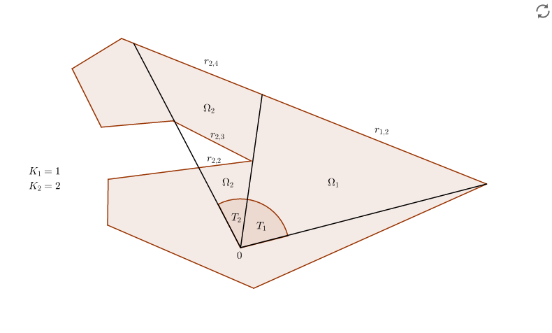
Figure 1: Construction of $\Omega_{i}$ and $r_{i,j}$

Proof.

Step 1. Let $Q=(0,\pi)^{n-2}\times(0,2\pi)$ and $H:Q\to S^{n-1}$ denote the hypershperical coordinates and $g(\varphi)d\varphi$ the surface element of $S^{n-1}$ in these coordinates, see Appendix, Section 5. By an approximation argument, using that $0\notin\partial\Omega$ and $a$ continuous, we can assume that $\Omega$ is of the following form (this is exactly the same as in [3] proof of Theorem 2.1, Step 3): there exists $\Omega_{i},$ $i=1,\ldots,l$ such that $\overline{\Omega}=\bigcup_{i=1}^{l}\Omega_{i}$, and each $\Omega_{i}$ is given in the following way (see Figure 1 giving an idea how to construct $\Omega_{i}$). We assume that there exists disjoint open subsets $T_{i}\subset Q,$ such that

$$\overline{Q}=\bigcup_{i=1}^{l}\overline{T}_{i}\,,$$

and for each $i=1,\ldots,l$ there exists $K_{i}\in\mathbb{N}$ and functions $r_{i,s}$ for $s=1,\ldots,2K_{i}$

$$r_{i,s}\in C^{1}\left(\overline{T}_{i}\right),\quad 0=r_{i,1}<r_{i,2}<\ldots<r_{i,2K_{i}},$$

such that

$$\Omega_{i}=\left\{rH(\varphi)|\;\varphi\in\overline{T}_{i}\,,\quad r_{i,2s-1}(\varphi)\leq r\leq r_{i,2s}(\varphi)\quad\text{ for }s=1,\ldots,K_{i}\right\}.$$

We can assume that $r_{i,1}=0$ because $0\in\Omega.$ Let $G$ denote the polar coordinates $G(t,\varphi)=tH(\varphi)$ (see Appendix) whose Jacobian determinant is given by $t^{n-1}g(\varphi).$ Therefore we obtain that

$$|\Omega_{i}|= \int_{T_{i}}\sum_{s=1}^{K_{i}}\int_{r_{i,2s-1}(\varphi)}^{r_{i,2s}(\varphi)}t^{n-1}g(\varphi)dt\,d\varphi=\int_{T_{i}}\sum_{s=1}^{K_{i}}\frac{1}{n}\left(r_{i,2s}^{n}-r_{i,2s-1}^{n}\right)g(\varphi)d\varphi\vskip 3.0pt plus 1.0pt minus 1.0pt$$

$$\geq \int_{T_{i}}\frac{1}{n}r_{i,2}^{n}(\varphi)g(\varphi)d\varphi.$$

Let us define a function $r:Q\to\mathbb{R},$ $\mathcal{H}^{n-1}$ almost eveywhere in $Q,$ by

$$r:\bigcup_{i=1}^{l}T_{i}\to\mathbb{R},\quad r(\varphi)=r_{i,2}(\varphi)\quad\text{if }\varphi\in T_{i}\,.$$

For $p\in S^{n-1}$ we set $\tilde{r}(p)=r(H^{-1}(p)),$ and thus $\tilde{r}(H(\varphi))=r(\varphi)$ almost everywhere in $Q.$ In this way we obtain that

$$|\Omega|=\sum_{i=1}^{l}|\Omega_{i}|\geq\frac{1}{n}\int_{Q}r(\varphi)^{n}g(\varphi)d\varphi=\frac{1}{n}\int_{S^{n-1}}\tilde{r}^{n}d\mathcal{H}^{n-1}.$$ (22)

Step 2. We now estimate the weighted perimeter. For $i=1,\ldots,l$ us define $\Gamma_{i}$ by

$$\Gamma_{i}=\bigcup_{s=2}^{2K_{i}}\left\{r_{i,s}(\varphi)H(\varphi)|\;\varphi\in\overline{T}_{i}\right\}.$$

In this way $\bigcup_{i=1}^{l}\Gamma_{i}\subset\partial\Omega$ and we obtain that

$$\int_{\partial\Omega}a(|x|)d\mathcal{H}^{n-1}(x)\geq\sum_{i=1}^{l}\int_{\Gamma_{i}}a(|x|)d\mathcal{H}^{n-1}(x)=\sum_{i=1}^{l}\sum_{s=2}^{2K_{i}}\int_{T_{i}}a(r_{i,s}(\varphi))\tilde{g}_{i,s}(\varphi)d\varphi,$$

where $\tilde{g}_{i,s}$ is given by

$$\tilde{g}_{i,s}(\varphi)=\sqrt{\det\left(\left\langle\frac{\partial F_{i,s}}{\partial\varphi_{j}},\frac{\partial F_{i,s}}{\partial\varphi_{k}}\right\rangle\right)_{j,k=1,\ldots,n-1}}$$ (23)

with the parametrizations $F_{i,s}(\varphi)=r_{i,s}(\varphi)H(\varphi).$ Using Lemma 17 and the fact that $a\geq 0,$ we obtain that

$$a\,\tilde{g}_{i,s}\geq a\,r_{i,s}^{n-1}g\quad\text{ for all $i,s.$}$$ (24)

It follows that

$$\int_{\partial\Omega}a(|x|)d\mathcal{H}^{n-1}(x)\geq\sum_{i=1}^{l}\sum_{s=2}^{2K_{i}}\int_{T_{i}}a(r_{i,s}(\varphi))r_{i,s}^{n-1}(\varphi)g(\varphi)d\varphi\geq\sum_{i=1}^{l}\int_{T_{i}}a(r_{i,2}(\varphi))r_{i,2}^{n-1}(\varphi)g(\varphi)d\varphi$$

Using again the definition of $r$ and $\tilde{r}$ introduced at the end of Step 1 we obtain

$$\int_{\partial\Omega}a(|x|)d\mathcal{H}^{n-1}(x)\geq\int_{S^{n-1}}a(\tilde{r})\tilde{r}^{n-1}d\mathcal{H}^{n-1}.$$ (25)

Step 3. Let us define $h$ by

$$h(t)=a\left(t^{\frac{1}{n}}\right)t^{\frac{n-1}{n}}.$$

It now follows from (22), from the fact that $h$ is decreasing, from Jensen inequality and finally (25), that

$$\begin{split}h\left(\frac{n|\Omega|}{\omega_{n-1}}\right)\leq&h\left(\frac{1}{\omega_{n-1}}\int_{S^{n-1}}\tilde{r}^{n}d\mathcal{H}^{n-1}\right)\leq\frac{1}{\omega_{n-1}}\int_{S^{n-1}}h\left(\tilde{r}^{n}\right)d\mathcal{H}^{n-1}\vskip 3.0pt plus 1.0pt minus 1.0pt\\ =&\frac{1}{\omega_{n-1}}\int_{S^{n-1}}a(\tilde{r})\tilde{r}^{n-1}d\mathcal{H}^{n-1}\leq\frac{1}{\omega_{n-1}}\int_{\partial\Omega}a(|x|)d\mathcal{H}^{n-1}(x).\end{split}$$ (26)

Since $|\Omega|=|B_{R}|$ one easily verifies that

$$R=\left(\frac{n|\Omega|}{\omega_{n-1}}\right)^{\frac{1}{n}}\quad\text{ and }\quad h\left(\frac{n|\Omega|}{\omega_{n-1}}\right)=a(R)R^{n-1}=\frac{1}{\omega_{n-1}}\int_{\partial B_{R}}a(|x|)d\mathcal{H}^{n-1}(x).$$ (27)

Plugging this identity into (26) concludes the proof inequality (21).

Step 4. We now deal with the case of equality in (21), first with the additional assumption that $\Omega$ is a $C^{1}$ set starshaped with respect to the origin: i.e. $\partial\Omega$ can be parametrized (up to a set of $\mathcal{H}^{n-1}$ measure zero) as $\partial\Omega=\{r(\varphi)H(\varphi)|\,\varphi\in Q\}.$ In other words $l=1,$ $K_{1}=1$ and $r=r_{1,2}\in C^{1}(Q).$ By hypothesis we must have equality in (22). Let us show that $r$ is constant. If $r$ is not constant, then by Lemma 17 there exists $\varphi_{0}$ and a neighborhood of $U$ in $Q$ containing $\varphi_{0}$ such that, recalling (23),

$$\tilde{g}_{1,1}>r^{n-1}g\quad\text{ in }U.$$

Thus we obtain a strict inequality in (25) and we cannot have equality in (21). (Note that if we additionally assume that $h$ is strictly convex, then equality in Jensen inequality also implies that $\tilde{r}$ must be constant.) We thus obtain that $\Omega$ is a ball centered at the origin with radius $r.$

Step 5. Let us treat now the general case of equality in (21). Since $\Omega$ is bounded there exsist $M>0$ such that

$$|x|\leq M\quad\text{ for all }x\in\partial\Omega\text{ and all }x\in\partial B_{R}\,.$$

Let us define $\tilde{a}$ by

$$\tilde{a}(t)=\left\{\begin{array}[]{rl}a(t)-a(M)&\text{ if }0<t\leq M\vskip 3.0pt plus 1.0pt minus 1.0pt\\ 0&\text{ if }t\geq M.\end{array}\right.$$

Note that $\tilde{a}$ is continuous and $\tilde{a}\geq 0,$ because $a$ is non-increasing (Remark 13). Moreover $\tilde{h}$ defined by

$$\tilde{h}(t)=\tilde{a}\big{(}t^{\frac{1}{n}}\big{)}t^{\frac{n-1}{n}}=\left\{\begin{array}[]{rl}a\big{(}t^{\frac{1}{n}}\big{)}t^{\frac{n-1}{n}}-a(M)t^{\frac{n-1}{n}}&\text{if }0<t^{\frac{1}{n}}\leq M\vskip 3.0pt plus 1.0pt minus 1.0pt\\ 0&\text{if }t^{\frac{1}{n}}\geq M\end{array}\right.$$

is non-increasing and convex, because it is the sum of two nonincreasing and convex functions. Therefore we can apply (21) to obtain that

$$\int_{\partial\Omega}\tilde{a}(|x|)d\mathcal{H}^{n-1}(x)\geq\int_{\partial B_{R}}\tilde{a}(|x|)d\mathcal{H}^{n-1}(x).$$

By the choice of $M$ and the definition of $\tilde{a}$ we have that $\tilde{a}(|x|)=a(|x|)-a(M)$ for any $x\in\partial\Omega\cup\partial B_{R}$. So the inequality becomes

$$\int_{\partial\Omega}a(|x|)d\mathcal{H}^{n-1}(x)-a(M)\mathcal{H}^{n-1}(\partial\Omega)\geq\int_{\partial B_{R}}a(|x|)d\mathcal{H}^{n-1}(x)-a(M)\mathcal{H}^{n-1}(\partial B_{R}).$$

Using now the assumption that we have equality in (21) and that $a(M)>0$, we obtain that $\mathcal{H}^{n-1}(\partial\Omega)\leq\mathcal{H}^{n-1}(\partial B_{R}).$ Which implies, in view of the classical isoperimetric inequality, that $\Omega$ must be a ball. Since $0\in\Omega$ we are in the case of the assumptions of Step 4 and the result follows. ∎

We will now prove Part (ii) of the main theorem. We will use the notation: if $x\in\mathbb{R}^{n}$ write $x=(x_{1},x^{\prime}),$ where $x^{\prime}\in\mathbb{R}^{n-1}.$

Proof of Theorem 9 Part (ii)..

Step 1. It is sufficient to find a sequence of sets $\Omega_{\epsilon}$ such that each $\Omega_{\epsilon}$ is Lipschitz, bounded, connected, $0\in\Omega_{\epsilon}$ and

$$\lim_{\epsilon\to 0}|\Omega_{\epsilon}|\to C>0\quad\text{ but }\quad\lim_{\epsilon\to 0}\int_{\partial\Omega_{\epsilon}}|x|^{p}d\mathcal{H}^{n-1}=0.$$ (28)

Then, by approximation, (28) holds also for a sequence of smooth sets. Then this sequence can be rescaled, defining a new sequence $\widehat{\Omega}_{\epsilon}=\lambda_{\epsilon}\Omega_{\epsilon}$ with $\lambda_{\epsilon}=C^{1/n}|\Omega_{\epsilon}|^{-1/n}$ so that $|\widehat{\Omega}_{\epsilon}|$ is constant and $\widehat{\Omega}_{\epsilon}$ still satisfies the second limit in (28).

Let us now show (28). Again by a rescaling argument, we can fix one $C$ and assume without loss of generality that $C=\alpha_{n}R^{n}$ for some $R>0.$ The idea is to choose $\Omega_{\epsilon}$ as a ball of radius $R$ and center going away to infinity, with a long and narrow cylinder attached to it so that it contains the origing, see Figure 2. One has to choose the length and radius of the cylinder carefully. More precisely: let us fix some $R>0$ define

$$c_{\epsilon}=\sqrt{R^{2}-\epsilon^{4}}+\epsilon^{-n+1}.$$

Then $\Omega_{\epsilon}$ shall be defined as the union of the following three sets: $\Omega_{\epsilon}=A_{\epsilon}\cup M_{\epsilon}\cup D_{\epsilon},$

$$A_{\epsilon}= \left\{x\in B_{\epsilon^{2}}^{n}:\,x_{1}\leq 0\right\}\vskip 3.0pt plus 1.0pt minus 1.0pt$$

$$M_{\epsilon}= \left(0,\epsilon^{-n+1}\right)\times B_{\epsilon^{2}}^{n-1}=\left\{x\in\mathbb{R}^{n}:\,0\leq x_{1}\leq\epsilon^{-n+1},\quad|x^{\prime}|<\epsilon^{2}\right\}\vskip 3.0pt plus 1.0pt minus 1.0pt$$

$$D_{\epsilon}= \left\{x\in\mathbb{R}^{n}:\,\left|x-\left(c_{\epsilon},0\right)\right|<R,\quad x_{1}\geq\epsilon^{-n+1}\right\}$$

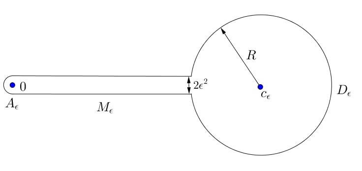
Figure 2: the domain $\Omega_{\epsilon}$

By construction $\Omega_{\epsilon}$ is a bounded connected Lipschitz set containing the origin. Note that

$$|A_{\epsilon}|=\frac{1}{2}\alpha_{n}\epsilon^{2n},\quad|M_{\epsilon}|=\frac{\alpha_{n-1}\epsilon^{2(n-1)}}{\epsilon^{n-1}}=\alpha_{n-1}\epsilon^{n-1}.$$

So we obtain that $\lim_{\epsilon\to 0}|\Omega_{\epsilon}|=\lim_{\epsilon\to 0}|D_{\epsilon}|=\alpha_{n}R^{n}.$

Step 2. It remains to estimate the weighted perimeter of $\partial\Omega_{\epsilon}.$ The contribution coming from $A_{\epsilon}$ is

$$\frac{1}{2}\int_{\partial B_{\epsilon^{2}}^{n}}|x|^{p}d\mathcal{H}^{n-1}=\frac{\omega_{n-1}}{2}\epsilon^{2(n-1)+2p}\to 0\quad\text{ for }\epsilon\to 0,$$

because $n+p-1>0.$ Note that for any $x\in\partial D_{\epsilon},$ we have the estimates, (since $p<0$), $|x|\geq\epsilon^{-n+1}$ and hence $|x|^{p}\leq\epsilon^{-p(n-1)}.$ This gives the estimate

$$\int_{\partial D_{\epsilon}}|x|^{p}d\mathcal{H}^{n-1}\leq\epsilon^{-p(n-1)}\omega_{n-1}R^{n-1}\to 0\quad\text{ for }\epsilon\to 0.$$

It remains to estimate the contribution coming from $M_{\epsilon}.$ It is equal to

$$\int_{0}^{\epsilon^{-n+1}}\int_{S_{\epsilon^{2}}^{n-2}}\left(x_{1}^{2}+|x^{\prime}|^{2}\right)^{\frac{p}{2}}d\mathcal{H}^{n-2}(x^{\prime})dx_{1}=\omega_{n-2}\epsilon^{2(n-2)}\int_{0}^{\epsilon^{-n+1}}\left(x_{1}^{2}+\epsilon^{4}\right)^{\frac{p}{2}}dx_{1}\vskip 3.0pt plus 1.0pt minus 1.0pt\\ =L_{1}+L_{2}\,,$$

where

$$L_{1}=\omega_{n-2}\epsilon^{2(n-2)}\int_{0}^{\epsilon^{2}}\left(x_{1}^{2}+\epsilon^{4}\right)^{\frac{p}{2}}dx_{1}\,\text{ and }\,L_{2}=\omega_{n-2}\epsilon^{2(n-2)}\int_{\epsilon^{2}}^{\epsilon^{-n+1}}\left(x_{1}^{2}+\epsilon^{4}\right)^{\frac{p}{2}}dx_{1}\,.$$

To estimate $L_{1}$ we just use that $x_{1}^{2}+\epsilon^{4}\geq\epsilon^{4},$ and that $p<0$ to get $L_{1}\leq\omega_{n-2}\epsilon^{2(n+p-1)}\to 0.$ To estimate $L_{2}$ we use that $x_{1}^{2}+\epsilon^{4}\geq x_{1}^{2}$ and therefore

$$L_{2}\leq\omega_{n-2}\epsilon^{2(n-2)}\int_{\epsilon^{2}}^{\epsilon^{-n+1}}x_{1}^{p}dx_{1}\,.$$

we distinguish 3 cases.

Case 1, $p>-1$. In this case $p+1>0$ and we obtain by explicit integration

$$L_{2}\leq\frac{\omega_{n-2}}{p+1}\epsilon^{2(n-2)}\left(\epsilon^{-(n-1)(p+1)}-\epsilon^{2(p+1)}\right)\leq\frac{\omega_{n-2}}{p+1}\epsilon^{2(n-2)-(n-1)(p+1)}.$$

So $L_{2}$ tends to zero as $\epsilon\to 0$ if and only if $2(n-2)-(n-1)(p+1)>0,$ which is equivalent to

$$p<\frac{n-3}{n-1}.$$

This is true, because $p<0$ and $n\geq 3.$

Case 2, $p=-1$. Explicit integration as in Case 1 gives that

$$L_{2}\leq-\omega_{n-2}(n+1)\epsilon^{2(n-2)}\log(\epsilon)\to 0,$$

because $n\geq 3.$

Case 3, $p<-1$. Hence $p+1<0$ and we obtain

$$L_{2}\leq-\frac{\omega_{n-2}}{p+1}\epsilon^{2(n-2)}\left(\epsilon^{2(p+1)}-\epsilon^{-(n-1)(p+1)}\right)\leq-\frac{\omega_{n-2}}{p+1}\epsilon^{2(n-2)+2(p+1)}\to 0,$$

using again that $n+p-1>0.$ ∎

Remark 14

Note that also Case 3 cannot occur if $n=2.$

We give here a proof of Theorem 9 (i) in the special case of starshaped domains, since it is quite short and contains a new and interesting interpolation argument due to Alvino et alt. [1]. The general case follows from a more standard, but weighted, symmetrization argument, see also [1].

Proposition 15

Let $n\geq 3,$ $0<p<1,$ $\Omega$ be a bounded open domain, starshaped with respect to the origin and with defining function $R$ (see (35) in Section 5) such that $R$ is Lipschitz. Then it holds that

$$n\alpha_{n}^{\frac{1-p}{n}}|\Omega|^{\frac{p+n-1}{n}}\leq\int_{\partial\Omega}|x|^{p}d\mathcal{H}^{n-1}.$$

Moreover, if there is equality then $\Omega$ has to be a ball centered at the origin.

Proof.

Step 1. Let us define by $P_{p}(\Omega)$ the right hand side of the inequality in the proposition. We abbreviate $S^{n-1}=S_{1}^{n-1},$ see (14) for notation. From Lemma 18 in the appendix we obtain that

$$P_{p}(\Omega):=\int_{\partial\Omega}|x|^{p}d\mathcal{H}^{n-1}=\int_{S^{n-1}}R^{p+n-1}\sqrt{1+\frac{1}{R^{2}}\left|\nabla_{S^{n-1}}R\right|^{2}}\,d\mathcal{H}^{n-1}.$$

Define

$$Z=R^{\frac{p+n-1}{n-1}}\quad\text{ and }\quad A=\left(\frac{n-1}{p+n-1}\right)^{2}\leq 1,$$

Note that for any $n\geq 3$ it holds that

$$1\geq A=\left(\frac{n-1}{p+n-1}\right)^{2}\geq\left(\frac{3-1}{p+3-1}\right)^{2}\geq 1-p\geq 0\quad\text{ for all }p\in[0,1].$$ (29)

From Lemma 19 and the previous inequality we obtain

$$\begin{split}P_{p}(\Omega)=&\int_{S^{n-1}}Z^{n-1}\sqrt{1+\frac{1}{Z^{2}}\left|\nabla_{S^{n-1}}Z\right|^{2}A}\,d\mathcal{H}^{n-1}\vskip 3.0pt plus 1.0pt minus 1.0pt\\ \geq&\int_{S^{n-1}}Z^{n-1}\sqrt{1+\frac{1}{Z^{2}}\left|\nabla_{S^{n-1}}Z\right|^{2}(1-p)}\,d\mathcal{H}^{n-1},\end{split}$$ (30)

Now use that for any $a,b\geq 0$ the mapping $t\mapsto\log\left[\int\sqrt{a+bt}\right]$ is concave, so that

$$\int\sqrt{a+b((1-p)t_{1}+pt_{2})}\geq\left(\int\sqrt{a+bt_{2}}\right)^{p}\left(\int\sqrt{a+bt_{1}}\right)^{1-p},\quad t_{1},t_{2}\geq 0.$$

Using this it follows from (30) (with $t_{1}=1,t_{2}=0)$

$$P_{p}(\Omega)\geq\left(\int_{S^{n-1}}Z^{n-1}d\mathcal{H}^{n-1}\right)^{p}\left(\int_{S^{n-1}}Z^{n-1}\sqrt{1+\frac{1}{Z^{2}}\left|\nabla_{S^{n-1}}Z\right|^{2}}\,d\mathcal{H}^{n-1}\right)^{1-p}$$ (31)

Define a new domain, also starshaped with respect to the origin,

$$\Omega^{Z}=\{0\}\cup\left\{x\in\mathbb{R}^{n}\backslash\{0\}\,:\,\frac{x}{|x|}=\theta\in S^{n-1},\,0<|x|<Z(\theta)\right\}.$$

It follows from Lemma 18, the standard isoperimetric inequality and (36) that

$$\int_{S^{n-1}}Z^{n-1} \sqrt{1+\frac{1}{Z^{2}}\left|\nabla_{S^{n-1}}Z\right|^{2}}\,d\mathcal{H}^{n-1}=\mathcal{H}^{n-1}(\partial\Omega^{Z})\geq\mathcal{L}^{n}(\Omega^{Z})^{\frac{n-1}{n}}n\alpha_{n}^{\frac{1}{n}}\vskip 3.0pt plus 1.0pt minus 1.0pt$$

$$= \left(\frac{1}{n}\int_{S^{n-1}}Z^{n}d\mathcal{H}^{n-1}\right)^{\frac{n-1}{n}}\alpha_{n}^{\frac{1}{n}}n=\left(\int_{S^{n-1}}Z^{n}d\mathcal{H}^{n-1}\right)^{\frac{n-1}{n}}(n\alpha_{n})^{\frac{1}{n}}.$$

We plug this into the (31) and use the definition of $Z$ to conclude that

$$P_{p}(\Omega)\geq\left(\int_{S^{n-1}}R^{p+n-1}d\mathcal{H}^{n-1}\right)^{p}\left(\int_{S^{n-1}}R^{\frac{(p+n-1)n}{n-1}}d\mathcal{H}^{n-1}\right)^{\frac{(1-p)(n-1)}{n}}(n\alpha_{n})^{\frac{1-p}{n}}.$$ (32)

The idea is to use now Hölder inequality in the form

$$\int_{S^{n-1}}R^{n}=\int_{S^{n-1}}R^{np}R^{n-np}\leq\left(\int_{S^{n-1}}R^{npq}\right)^{\frac{1}{q}}\left(\int_{S^{n-1}}R^{(n-np)q^{\prime}}\right)^{\frac{1}{q^{\prime}}}$$ (33)

with $1<q<\infty,$

$$q=\frac{p+n-1}{pn},\quad q^{\prime}=\frac{p+n-1}{(n-1)(1-p)},\quad\frac{1}{q}+\frac{1}{q^{\prime}}=1.$$

We take (33) to the power $(p+n-1)/n$ and multiply by $(n\alpha_{n})^{(1-p)/n}$ to get (using (32) in the last step)

$$(n\alpha_{n})^{\frac{1-p}{n}} \left(\int_{S^{n-1}}R^{n}d\mathcal{H}^{n-1}\right)^{\frac{p+n-1}{n}}\vskip 3.0pt plus 1.0pt minus 1.0pt$$

$$\leq (n\alpha_{n})^{\frac{1-p}{n}}\left(\int_{S^{n-1}}R^{p+n-1}d\mathcal{H}^{n-1}\right)^{\frac{p+n-1}{nq}}\left(\int_{S^{n-1}}R^{\frac{n(p+n-1)}{n-1}}d\mathcal{H}^{n-1}\right)^{\frac{p+n-1}{nq^{\prime}}}\vskip 3.0pt plus 1.0pt minus 1.0pt$$

$$= (n\alpha_{n})^{\frac{1-p}{n}}\left(\int_{S^{n-1}}R^{p+n-1}d\mathcal{H}^{n-1}\right)^{p}\left(\int_{S^{n-1}}R^{\frac{n(p+n-1)}{n-1}}d\mathcal{H}^{n-1}\right)^{\frac{(1-p)(n-1)}{n}}\vskip 3.0pt plus 1.0pt minus 1.0pt$$

$$\leq P_{p}(\Omega).$$

Thus it follows from (36) that

$$n\alpha_{n}^{\frac{1-p}{n}}|\Omega|^{\frac{p+n-1}{n}}=(n\alpha_{n})^{\frac{1-p}{n}}\left(\int_{S^{n-1}}R^{n}d\mathcal{H}^{n-1}\right)^{\frac{p+n-1}{n}}\leq P_{p}(\Omega),$$

which proves the first part of the proposition.

Step 2. Let us consider the case of equality. In that case there must be equality in (33), which is only possible if for some constant $c\in\mathbb{R}$

$$R(\theta)^{p+n-1}=cR(\theta)^{\frac{n(p+n-1)}{n-1}}\quad\text{ for all }\theta\in S^{n-1}.$$

This is only possible if $R$ is constant. ∎

Remark 16

The present proof does not work for $n=2,$ since in that case (29) is not satisfied for all $p\in(0,1).$

5 Appendix: hyperspherical coordinates in $\mathbb{R}^{n}.$

We have used in Section 4 the explicit form of hyperspherical coordinates and their properties. Let us define $Q\subset\mathbb{R}^{n-1}$ by

$$Q=(0,\pi)^{n-2}\times(0,2\pi).$$

The hypershperical coordinates $H=(H_{1},\ldots,H_{n}):Q\to S^{n-1}\subset\mathbb{R}^{n}$ are defined as: for $k=1,\ldots,n$ and $\varphi=(\varphi_{1},\ldots,\varphi_{n-1})$

$$H_{k}(\varphi)=\cos\varphi_{k}\prod_{l=0}^{k-1}\sin\varphi_{l}\quad\text{ with convention }\varphi_{0}=\frac{\pi}{2},\quad\varphi_{n}=0.$$

A calculation shows that $d_{i}(\varphi):=\left\langle\frac{\partial H}{\partial\varphi_{i}},\frac{\partial H}{\partial\varphi_{i}}\right\rangle=\prod_{l=0}^{i-1}\sin^{2}\varphi_{l}>0.$ One verifies that the metric tensor $S^{n-1}$ in these coordinates is diagonal $g_{ij}(\varphi)=\left\langle\frac{\partial H}{\partial\varphi_{i}},\frac{\partial H}{\partial\varphi_{j}}\right\rangle=\delta_{ij}d_{i}(\varphi),$ ($\delta_{ij}=1$ if $i=j$ and $0$ else) and hence the surface element $g$ is given by

$$g(\varphi)=\sqrt{\det g_{ij}(\varphi)}=\prod_{k=1}^{n-1}d_{k}(\varphi)=\prod_{k=1}^{n-2}(\sin\varphi_{k})^{n-k-1}.$$

Let us also denote the polar coordinates in $\mathbb{R}^{n},$ denoted as $G:(0,\infty)\times Q\to\mathbb{R}^{n},$ given by $G(t,\varphi)=tH(\varphi).$ Its Jacobian determinant is then given by

$$\det DG(t,\varphi)=t^{n-1}g(\varphi).$$ (34)

For our purpose the following lemma will be useful.

Lemma 17

Suppose $T\subset Q$ is an open set and a hypersurface $\Gamma\subset\mathbb{R}^{n}$ is given by the parametrization $F:T\to\Gamma$

$$F(\varphi)=r(\varphi)H(\varphi),$$

where $r$ is some smooth function $r:T\to(0,\infty).$ The surface element in this parametrization calculates as

$$\det\left(\left\langle\frac{\partial F}{\partial\varphi_{i}},\frac{\partial F}{\partial\varphi_{j}}\right\rangle\right)_{i,j=1,\ldots,n-1}=r^{2n-4}\left(\sum_{i=1}^{n-1}\Big{(}\frac{\partial r}{\partial\varphi_{i}}\Big{)}^{2}d_{1}\cdots\widehat{d_{i}}\cdots d_{n-1}+r^{2}\prod_{i=1}^{n-1}d_{i}\right),$$

where $\widehat{d_{i}}$ means that $d_{i}$ should be omitted in the product. In particular, since $d_{i}>0,$ the surface element is bigger than $r^{n-1}g(\varphi).$

Proof.

Using the relations $\langle H;H\rangle=1$ and $\left\langle H;\frac{\partial H}{\partial\varphi_{i}}\right\rangle=0,$ one obtains that

$$M_{ij}:=\left\langle\frac{\partial F}{\partial\varphi_{i}},\frac{\partial F}{\partial\varphi_{j}}\right\rangle=\frac{\partial r}{\partial\varphi_{i}}\frac{\partial r}{\partial\varphi_{j}}+r^{2}g_{ij}=\frac{\partial r}{\partial\varphi_{i}}\frac{\partial r}{\partial\varphi_{j}}+r^{2}\delta_{ij}d_{i}\,.$$

Thus the matrix $M$ with entries $M_{ij}$ is of the form $M=A+r^{2}D$ where $A$ has rank $1$ and $D$ is diagonal with entries $d_{i}$. Thus using the linearity of the determinant in the columns one obtains that (since no matrix with two columns of $A$ survives when developing the determinant succesively with respect to the columns)

$$\det M=\sum_{i=1}^{n-1}\det\widehat{A_{i}}+\det r^{2}D,$$

where $\widehat{A_{i}}$ is the matrix obtained from $r^{2}D$ by replacing the $i$-th column of $r^{2}D$ by the $i$-th column of $A.$ From this the lemma follows. ∎

We now use the hypershperical coordinates to deal with domains starshaped with respect to the origin. By definition, a bounded open Lipschitz domain $\Omega\in\mathbb{R}^{n}$ is starshaped with respect to the origin if there exists a function $R:S^{n-1}\to(0,\infty)$ such that

$$\Omega=\{0\}\cup\left\{x\in\mathbb{R}^{n}\backslash\{0\}\,:\,\frac{x}{|x|}=\theta\in S^{n-1},\,0<|x|<R(\theta)\right\}$$ (35)

We shall call $R$ the defining function of $\Omega.$ Note that $R$ is not necessarily Lipschitz, even if $\Omega$ is, and it might even be discontinuous (for example $\Omega=\left(B_{r_{2}}(0)\cap\{x_{2}>0\}\right)\cup\left(B_{r_{1}}(0)\cap\{x_{2}<0\}\right)\subset\mathbb{R}^{2},$ with $r_{1}<r_{2}$). But we will alway assume that $R$ is also Lipschitz. It follows from the relation (34) that the volume of a starshaped domain calculates as

$$\mathcal{L}^{n}(\Omega)=\frac{1}{n}\int_{S^{n-1}}R^{n}d\mathcal{H}^{n-1}$$ (36)

For an almost everywhere differentiable function $f:S^{n-1}\to\mathbb{R}$ we recall that the norm of the covariant gradient of $f$ at $p$ on the manifold $S^{n-1}$ can be calculated as

$$\left|\nabla_{S^{n-1}}f\right|^{2}=\sum_{i=1}^{n-1}\left|\nabla_{E_{i}}f\right|^{2},$$ (37)

where $\left\{E_{1},\ldots,E_{n-1}\right\}$ is any orthonormal basis of $T_{p}S^{n-1},$ and $\nabla_{E}f$ is the derivative in direction $E.$

Lemma 18

Let $\Omega\subset\mathbb{R}^{n}$ be a bounded open Lipschitz set, starshaped with respect to the origin and defining function $R$ as in (35). Assume also that $R$ is Lipschitz. Then for any continuous function $g:(0,\infty)\to\mathbb{R}$ it holds that

$$\int_{\partial\Omega}g(|x|)d\mathcal{H}^{n-1}(x)=\int_{S^{n-1}}(g\circ R)R^{n-1}\sqrt{1+\frac{1}{R^{2}}\left|\nabla_{S^{n-1}}R\right|^{2}}d\mathcal{H}^{n-1}.$$ (38)

The assumption that $g$ is continuous can be reduced, but we will need the lemma only for $g(t)=t^{p}.$

Proof.

We use the hyperspherical coordinates $H,$ definitions of $d_{i}$ and $g,$ respectively their properties (summarized in the beginning of this section). Let $\varphi\in Q,$ $p=H(\varphi)$ and

$$d_{i}(\varphi)=\left|\frac{\partial H}{\partial\varphi_{i}}\right|^{2},\quad\text{ then }\quad E_{i}(p)=\frac{1}{\sqrt{d_{i}(\varphi)}}\frac{\partial H}{\partial\varphi_{i}},\quad i=1,\ldots,n-1$$

form an orthonormal basis of $T_{p}S^{n-1}.$ Thus we obtain from (37) (we can assume that $R$ has been extended to a neighborhood of $S^{n-1}$) that at $p=H(\varphi)$

$$\begin{split}\left|\nabla_{S^{n-1}}R\right|^{2}=&\sum_{i=1}^{n-1}\frac{1}{d_{i}(\varphi)}\Big{|}\Big{\langle}\nabla R(H(\varphi));\frac{\partial H}{\partial\varphi_{i}}\Big{\rangle}\Big{|}^{2}=\sum_{i=1}^{n-1}\frac{1}{d_{i}(\varphi)}\Big{[}\frac{\partial}{\partial\varphi_{i}}(R\circ H)\Big{]}^{2}\vskip 3.0pt plus 1.0pt minus 1.0pt\\ =&\sum_{i=1}^{n-1}\frac{1}{d_{i}(\varphi)}\Big{[}\frac{\partial r}{\partial\varphi_{i}}\Big{]}^{2}\end{split}$$ (39)

where we define for $\varphi\in Q$

$$r(\varphi):=R(H(\varphi))\quad\text{ and }\quad F(\varphi)=r(\varphi)H(\varphi).$$

Hence $F:Q\to\partial\Omega$ is a parametrization of $\partial\Omega.$ Using Lemma 17 we obtain that

$$\sqrt{\det\Big{(}\Big{\langle}\frac{\partial F}{\partial\varphi_{i}},\frac{\partial F}{\partial\varphi_{j}}\Big{\rangle}\Big{)}}= r^{n-1}\sqrt{d_{1}d_{2}\cdots d_{n-1}}\sqrt{1+\frac{1}{r^{2}}\sum_{i=1}^{n-1}\frac{1}{d_{i}}\Big{(}\frac{\partial r}{\partial\varphi_{i}}\Big{)}^{2}}\vskip 3.0pt plus 1.0pt minus 1.0pt$$

$$= r^{n-1}\sqrt{1+\frac{1}{r^{2}}\sum_{i=1}^{n-1}\frac{1}{d_{i}}\Big{(}\frac{\partial r}{\partial\varphi_{i}}\Big{)}^{2}}\,g(\varphi).$$

Therefore, using the parametrization $F$ to calculate the left side of (38), respectively the parametrization $H$ to calculate the right side and (39), the lemma follows. ∎

Lemma 19

Let $R$ be a Lipschitz function, mapping $S^{n-1}$ to $(0,\infty),$ $\alpha\in\mathbb{R}$ and define $Z:S^{n-1}\to\mathbb{R}$ by $Z=R^{\alpha}.$ Then the following identity holds

$$\alpha^{2}\frac{1}{R^{2}}\left|\nabla_{S^{n-1}}R\right|^{2}=\frac{1}{Z^{2}}\left|\nabla_{S^{n-1}}Z\right|^{2}.$$

In particular if $p\in\mathbb{R}$ is such that $p+n-1\neq 0$ and

$$Z=R^{\frac{p+n-1}{n-1}},$$

then

$$R^{p+n-1}\sqrt{1+\frac{1}{R^{2}}\left|\nabla_{S^{n-1}}R\right|^{2}}=Z^{n-1}\sqrt{1+\frac{1}{Z^{2}}\left|\nabla_{S^{n-1}}Z\right|^{2}\left(\frac{n-1}{p+n-1}\right)^{2}}$$

Proof.

Let $E\in T_{p}S^{n-1}$ be a tangent vector. Then we get

$$\nabla_{E}Z=\langle\nabla Z,E\rangle=\alpha R^{\alpha-1}\langle\nabla R,E\rangle$$

and it follows from (37) that $|\nabla_{S^{n-1}}Z|^{2}=\alpha^{2}R^{2\alpha-2}|\nabla_{S^{n-1}}R|^{2}.$ From this the lemma follows easily. ∎

Acknowledgements The author was supported by the Chilean Fondecyt Iniciación grant nr. 11150017. He would also like to thank Friedemann Brock for some helpful discussions related to the simplification of the proofs in [1].

References

- [1] A. Alvino, F. Brock, F. Chiacchio, A. Mercaldo and M.R. Posteraro, Some isoperimetric inequalities on with respect to weights , J. Math. Anal. Appl. (2017) http://dx.doi.org/10.1016/j.jmaa.2017.01.085.
- [2] Adimurthi A. and Sandeep K., A singular Moser-Trudinger embedding and its applications, NoDEA Nonlinear Differential Equations Appl., 13 (2007), no. 5-6, 585–603.
- [3] Betta M.F., Brock F., Mercaldo A. and Posteraro M.R., A weighted isoperimetric inequality and applications to symmetrization, J. of Inequal. and Appl., 4 (1999), 215–240.
- [4] Boyer W., Brown B., Chambers G.R., Loving A. and Tammen S., Isoperimetric Regions in with density arXiv:1504.01720.
- [5] Bayle V., Cañete A. , Morgan F. and Rosales C., On the isoperimetric problem in Euclidean space with density, Calc. Var. Partial Differential Equations 31 (2008), no. 1, 27–46.
- [6] Cabré X. and Ros-Oton X., Sobolev and isoperimetric inequalities with monomial weights, J. Differential Equations 255 (2013), no. 11, 4312–4336.
- [7] Cabré X., Ros-Oton X. and Serra J., Euclidean balls solve some isoperimetric problems with nonradial weights, C. R. Math. Acad. Sci. Paris 350 (2012), no. 21-22, 945–947.
- [8] Cañete A., Miranda M. and Vittone D., Some isoperimetric problems in planes with density, J. Geom. Anal., 20 (2010), no. 2, 243–290.
- [9] Carroll C., Jacob A. Adam, Quinn C. and Walters R., The isoperimetric problem on planes with density, Bull. Aust. Math. Soc., 78 (2008), no. 2, 177–197.
- [10] Chambers G.R., Proof of the log-convex density conjecture, arXiv:1311.4012.
- [11] Csató G., An isoperimetric problem with density and the Hardy-Sobolev inequality in , Differential Integral Equations, 28 (2015), no. 9/10, 971–988.
- [12] Csató G. and Roy P., Extremal functions for the singular Moser-Trudinger inequality in 2 dimensions, Calc. Var. Partial Differential Equations, 54 (2015), no. 2, 2341–2366.
- [13] Csató G. and Roy P., The singular Moser-Trudinger inequality on simply connected domains, Communications in Partial Differential Equations, to appear.
- [14] Dahlberg J., Dubbs A., Newkirk E. and Tran H., Isoperimetric regions in the plane with density , New York J. Math., 16 (2010), 31–51.
- [15] Díaz A., Harman N., Howe S. and Thompson D., Isoperimetric problems in sectors with density, Adv. Geom., 12 (2012), 589–619.
- [16] Barbosa J.L. and do Carmo M., Stability of hypersurfaces with constant mean curvature, Math. Z., 185 (1984), no. 3, 339–353.
- [17] Figalli A. and Maggi F., On the isoperimetric problem for radial log-convex densities, Calc. Var. Partial Differential Equations, 48 (2013), no. 3-4, 447–489.
- [18] Flucher M., Extremal functions for the Trudinger-Moser inequality in 2 dimensions, Comment. Math. Helvetici, 67 (1992), 471–497.
- [19] Fusco N., Maggi F. and Pratelli A., On the isoperimetric problem with respect to a mixed Euclidean-Gaussian density, J. Funct. Anal., 260 (2011), no. 12, 3678–3717.
- [20] Di Giosia L., Habib J., Kenigsberg L., Pittman D and Zhu W, Balls Isoperimetric in with Volume and Perimeter Densities and , arXiv:1610.05830v1.
- [21] Morgan F., Regularity of isoperimetric hypersurfaces in Riemannian manifolds, Trans. Amer. Math. Soc., 355 (2003), no. 12, 5041–5052.
- [22] Morgan F., http://sites.williams.edu/Morgan/2010/06/22/variation-formulae-for-perimeter-and-volume-densities/.
- [23] Morgan F. and Pratelli A., Existence of isoperimetric regions in with density, Ann. Global Anal. Geom., 43 (2013), no. 4, 331–365.
- [24] Walter W., Ordinary differential equations, English translation, Springer, 1998.