A Note on Some Approximation Kernels on the Sphere

Abstract

We produce precise estimates for the Kogbetliantz kernel for the approximation of functions on the sphere. Furthermore, we propose and study a new approximation kernel, which has slightly better properties.

Dedicated to Ian H. Sloan on the occasion of his 80^th birthday.

1 Introduction

For $d\geq 1$, let ${\mathbb{S}}^{d}=\{\mathbf{z}\in{\mathbb{R}}^{d+1}:\langle\mathbf{z},\mathbf{z}\rangle=1\}$ denote the $d$-dimensional unit sphere embedded in the Euclidean space ${\mathbb{R}}^{d+1}$ and $\langle\cdot,\cdot\rangle$ be the usual inner product. We use $\mathrm{d}\sigma_{d}$ for the surface element and set $\omega_{d}=\int_{{\mathbb{S}}^{d}}\mathrm{d}\sigma_{d}$.

In Kogbetliantz1924:recherches_sommabilite E. Kogbetliantz studied Cesàro means of the ultraspherical Dirichlet kernel. Let $C_{n}^{\lambda}$ denote the $n$-th Gegenbauer polynomial of index $\lambda$. Then for $\lambda=\frac{d-1}{2}$

$$K_{n}^{\lambda,0}(\langle\mathbf{x},\mathbf{y}\rangle)=\sum_{k=0}^{n}\frac{k+\lambda}{\lambda}C_{k}^{\lambda}(\langle\mathbf{x},\mathbf{y}\rangle)$$

is the projection kernel on the space of harmonic polynomials of degree $\leq n$ on the sphere $\mathbb{S}^{d}$. The kernel could be studied for all $\lambda>0$, but since we have the application to polynomial approximation on the sphere in mind, we restrict ourselves to half-integer and integer values of $\lambda$. Throughout this paper $d$ will denote the dimension of the sphere and $\lambda=\frac{d-1}{2}$ will be the corresponding Gegenbauer parameter.

Kogbetliantz Kogbetliantz1924:recherches_sommabilite studied how higher Cesàro-means improve the properties of the kernel $K_{n}^{\lambda,0}$: for $\alpha\geq 0$ set

$$K_{n}^{\lambda,\alpha}(t)=\frac{1}{\binom{n+\alpha}{n}}\sum_{k=0}^{n}\binom{n-k+\alpha}{n-k}\frac{k+\lambda}{\lambda}C_{k}^{\lambda}(t).$$

He proved that the kernels $(K_{n}^{\lambda,\alpha})_{n}$ have uniformly bounded $L^{1}$-norm, if $\alpha>\lambda$ and that they are non-negative, if $\alpha\geq 2\lambda+1$. There is a very short and transparent proof of the second fact due to Reimer Reimer1996:kogbetliantz_cesaro . In this paper, we will restrict our interest to the kernel $K_{n}^{\lambda,2\lambda+1}$, which we will denote by $K_{n}^{\lambda}$ for short.

The purpose of this note is to improve Kogbetliantz’ upper bounds for the kernel $K_{n}^{\lambda}$. Especially, the estimates for $K_{n}^{\lambda}(t)$ given in Kogbetliantz1924:recherches_sommabilite exhibit rather bad behaviour at $t=-1$. This is partly a consequence of the actual properties of the kernel at that point, but to some extent the estimate used loses more than necessary. Furthermore, the estimates given in Kogbetliantz1924:recherches_sommabilite contain unspecified constants. We have used some effort to provide good explicit constants.

In the end of this paper we will propose a slight modification of the kernel function, which is better behaved at $t=-1$ and still shares all desirable properties of $K_{n}^{\lambda}$.

2 Estimating the kernel function

In the following we will use the notation

$$A_{n}^{\alpha}=\binom{n+\alpha}{n}.$$

Notice that

$$\sum_{n=0}^{\infty}A_{n}^{\alpha}z^{n}=\frac{1}{(1-z)^{\alpha+1}}.$$ (1)

Let $C_{n}^{\lambda}$ denote the $n$-th Gegenbauer polynomial with index $\lambda$. The Gegenbauer polynomials satisfy two basic generating function relations (cf. Andrews_Askey_Roy1999:special_functions ; Kogbetliantz1924:recherches_sommabilite )

$$\sum_{n=0}^{\infty}C_{n}^{\lambda}(\cos\vartheta)z^{n} =\frac{1}{(1-2z\cos\vartheta+z^{2})^{\lambda}}$$ (2)

$$\sum_{n=0}^{\infty}\frac{n+\lambda}{\lambda}C_{n}^{\lambda}(\cos\vartheta)z^{n} =\frac{1-z^{2}}{(1-2z\cos\vartheta+z^{2})^{\lambda+1}}.$$ (3)

Several different kernel functions for approximation of functions on the sphere and their saturation behaviour have been studied in Berens_Butzer_Pawelke1969:limitierungsverfahren_kugelfunktionen . We will investigate the kernel

$$K_{n}^{\lambda}(\cos\vartheta)=\frac{1}{A_{n}^{2\lambda+1}}\sum_{k=0}^{n}A_{n-k}^{2\lambda+1}\frac{k+\lambda}{\lambda}\,C_{k}^{\lambda}(\cos\vartheta),$$

which has been shown to be positive by E. Kogbetliantz Kogbetliantz1924:recherches_sommabilite for $\lambda>0$.

By the generating functions (1) and (3) it follows

$$\sum_{n=0}^{\infty}A_{n}^{2\lambda+1}K_{n}^{\lambda}(\cos\vartheta)z^{n}=\frac{1+z}{(1-2z\cos\vartheta+z^{2})^{\lambda+1}(1-z)^{2\lambda+1}}.$$ (4)

Thus we can derive integral representations for $K_{n}^{\lambda}$ using Cauchy’s integral formula. As pointed out in the introduction, we will restrict the values of $\lambda$ to integers or half-integers. The main advantage of this is the fact that the exponent of $(1-z)$ in (4) is then an integer.

For $\lambda=k\in\mathbb{N}_{0}$ we split the generating function (4) into two factors

$$\frac{1+z}{(1-2z\cos\vartheta+z^{2})(1-z)}\times\frac{1}{(1-2z\cos\vartheta+z^{2})^{k}(1-z)^{2k}}.$$

The first factor is essentially the generating function of the Fejér kernel, namely

$$\frac{1}{2\pi i}\oint\limits_{|z|=\frac{1}{2}}\frac{1+z}{(1-2z\cos\vartheta+z^{2})(1-z)}\frac{\mathrm{d}z}{z^{n+1}}=\left(\frac{\sin(n+1)\frac{\vartheta}{2}}{\sin\frac{\vartheta}{2}}\right)^{2}\leq\frac{1}{(\sin\frac{\vartheta}{2})^{2}}.$$ (5)

Notice that this is just the kernel $(n+1)K_{n}^{0}$.

We compute the coefficients of the second factor using Cauchy’s formula

$$Q_{n}^{k}(\cos(\vartheta))=\frac{1}{2\pi i}\oint\limits_{|z|=\frac{1}{2}}\frac{1}{(1-2z\cos\vartheta+z^{2})^{k}(1-z)^{2k}}\frac{\mathrm{d}z}{z^{n+1}}.$$ (6)

In order to produce an estimate for $Q_{n}^{k}$, we first compute $Q_{n}^{1}$. This is done by residue calculus and yields

$$Q_{n}^{1}(\cos(\vartheta))=\frac{1}{4\sin^{2}(\frac{\vartheta}{2})}\left(n+2-\frac{\sin((n+2)\vartheta)}{\sin(\vartheta)}\right).$$ (7)

This function is obviously non-negative and satisfies

$$Q_{n}^{1}(\cos(\vartheta))\leq\frac{n+2}{2\sin^{2}(\frac{\vartheta}{2})}.$$ (8)

Now the functions $Q_{n}^{k}$ are formed from $Q_{n}^{1}$ by successive convolution:

$$Q_{n}^{k+1}(\cos(\vartheta))=\sum_{m=0}^{n}Q_{m}^{k}(\cos(\vartheta))Q_{n-m}^{1}(\cos(\vartheta)).$$

Inserting the estimate (8) and an easy induction yields

$$Q_{n}^{k}(\cos(\vartheta))\leq\frac{1}{2^{k}\sin^{2k}(\frac{\vartheta}{2})}\sum_{r=0}^{k}\binom{k}{r}\binom{n+r+k-1}{n}.$$ (9)

Remark 1

Asymptotically, this estimate is off by a factor of $2^{\lambda}$, but as opposed to Kogbetliantz’ estimate it does not contain a negative power of $\sin(\vartheta)$, which would blow up at $\vartheta=\pi$. The size of the constant is lost in the transition from (7) to (8), where the trigonometric term (actually a Chebyshev polynomial of the second kind) is estimated by its maximum. On the one hand this avoids a power of $\sin(\vartheta)$ in the denominator, on the other hand it spoils the constant.

Putting (5) and (9) together yields

$$A_{n}^{2k+1}K_{n}^{k}(\cos(\vartheta))\leq\frac{1}{2^{k}(\sin\frac{\vartheta}{2})^{2k+2}}\sum_{\ell=0}^{k}\binom{k}{\ell}\binom{n+k+\ell}{n},$$ (10)

where we have used the identity

$$\sum_{i=0}^{n}\binom{i+m}{i}=\binom{n+m+1}{n}.$$

Remark 2

Since the generating function of $A_{n}^{2k+1}K_{n}^{k}(\cos(\vartheta))$ is a rational function in this case, an application of residue calculus would have of course been an option. The calculation of the residues at $e^{\pm i\vartheta}$ produces a denominator containing $\sin(\vartheta)^{2k-1}$. Computation of the numerators for small values of $k$ show that this denominator actually cancels, but we did not succeed in proving this in general. Furthermore, keeping track of the estimates through this cancellation seems to be difficult. This denominator could also be eliminated by restricting $\frac{C}{n}\leq\vartheta\leq\pi-\frac{C}{n}$, but this usually spoils any gain in the constants obtained before. This was actually the technique used in Kogbetliantz1924:recherches_sommabilite .

For $\lambda=\frac{1}{2}+k$ we split the generating function (4) into the factors

$$\frac{1}{\sqrt{1-2z\cos\vartheta+z^{2}}(1-z)}\times\frac{1+z}{(1-2z\cos\vartheta+z^{2})^{k+1}(1-z)^{2k+1}}$$ (11)

with $k\in\mathbb{N}_{0}$. The second factor is exactly the generating function related to the case of integer parameter $\lambda$ studied above.

For the coefficients of the first factor in (11) we use Cauchy’s formula again

$$R_{n}(\cos\vartheta)=\frac{1}{2\pi i}\oint\limits_{|z|=\frac{1}{2}}\frac{1}{\sqrt{1-2z\cos\vartheta+z^{2}}(1-z)}\frac{\mathrm{d}z}{z^{n+1}}.$$

Figure 1: The contour of integration used for deriving $R_{n}(\cos\vartheta)$.

We deform the contour of integration to encircle the branch cut of the square root, which is chosen to be the arc of the circle of radius one connecting the points $e^{\pm i\vartheta}$ passing through $-1$. This deformation of the contour passes through $\infty$ and the simple pole at $z=1$, where we collect a residue. This gives

$$R_{n}(\cos\vartheta)=\frac{1}{2\sin\frac{\vartheta}{2}}-\frac{1}{2\sqrt{2}\pi}\int\limits_{\vartheta}^{2\pi-\vartheta}\frac{\cos((n+1)\vartheta)}{\sqrt{\cos\vartheta-\cos t}\sin\frac{t}{2}}\,\mathrm{d}t.$$

We estimate this by

$$R_{n}(\cos\vartheta)\leq\frac{1}{2\sin\frac{\vartheta}{2}}+\frac{1}{2\sqrt{2}\pi}\int\limits_{\vartheta}^{2\pi-\vartheta}\frac{1}{\sqrt{\cos\vartheta-\cos t}\sin\frac{t}{2}}\,\mathrm{d}t=\frac{1}{\sin\frac{\vartheta}{2}}.$$ (12)

This estimate is the best possible independent of $n$, because $R_{2n}(-1)=1$.

Putting the estimates (10) and (12) together we obtain

$$A_{n}^{2k+2}K_{n}^{k+\frac{1}{2}}(\cos(\vartheta))\leq\frac{1}{2^{k}(\sin(\frac{\vartheta}{2}))^{2k+3}}\sum_{\ell=0}^{k}\binom{k}{\ell}\binom{n+k+\ell+1}{n}.$$ (13)

Summing up, we have proved the following.

Theorem 2.1

Let $\lambda=\frac{d-1}{2}$ be a positive integer or half-integer. Then the kernel $K_{n}^{\lambda}$ satisfies the following estimates

$$K_{n}^{\lambda}(\cos\vartheta)\leq\begin{cases}\displaystyle{\frac{1}{2^{\lfloor\lambda\rfloor}(\sin(\frac{\vartheta}{2}))^{2\lambda+2}}\sum_{\ell=0}^{\lfloor\lambda\rfloor}\binom{\lfloor\lambda\rfloor}{\ell}\frac{(2\lambda+1)_{\ell+1}}{(n+2\lambda+1)_{\ell+1}}}&\text{for}\quad 0<\vartheta\leq\pi\\[17.07164pt] \frac{(n+4\lambda+1)_{n}}{(n+2\lambda)_{n}}&\text{for}\quad 0\leq\vartheta\leq\pi,\end{cases}$$ (14)

where $(a)_{n}=a(a-1)\cdots(a-n+1)$ denotes the falling factorial (Pochhammer symbol).

Remark 3

The estimate (14) is best possible with respect to the behaviour in $n$ for a fixed $\vartheta\in(0,\pi)$, as well as for the power of $\sin\frac{\vartheta}{2}$. The constant in front of the main asymptotic term could still be improved, especially its dependence on the dimension. The second estimate is the trivial estimate by $K_{n}^{\lambda}(1)$.

3 A new kernel

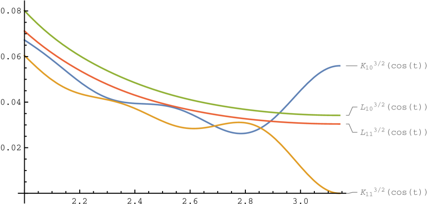
Figure 2: Comparison between the kernels $K_{10}^{\frac{3}{2}}$, $K_{11}^{\frac{3}{2}}$, $L_{10}^{\frac{3}{2}}$, and $L_{11}^{\frac{3}{2}}$. The kernels $K$ show oscillations and a parity phenomenon at $\vartheta=\pi$.

The kernel $K_{n}^{\lambda}(\cos\vartheta)$ exhibits a parity phenomenon at $\vartheta=\pi$, which occurs in the first asymptotic order term (see Figure 2 for illustration). This comes from the fact that the two singularities at $e^{\pm i\vartheta}$ collapse to one singularity of twice the original order for this value of $\vartheta$. In order to avoid this, we propose to study the kernel given by the generating function

$$\frac{(1+z)^{2\lambda+2}}{(1-2z\cos\vartheta+z^{2})^{\lambda+1}(1-z)^{2\lambda+1}}=\frac{1-z^{2}}{(1-2z\cos\vartheta+z^{2})^{\lambda+1}}\times\frac{(1+z)^{2\lambda+1}}{(1-z)^{2\lambda+2}}.$$ (15)

Let $B_{n}^{\lambda}$ be given by

$$\sum_{n=0}^{\infty}B_{n}^{\lambda}z^{n}=\frac{(1+z)^{2\lambda+1}}{(1-z)^{2\lambda+2}},$$ (16)

then the kernel is given by

$$L_{n}^{\lambda}(\cos\vartheta) =\frac{1}{B_{n}^{\lambda}}\sum_{k=0}^{n}B_{n-k}^{\lambda}\frac{k+\lambda}{\lambda}C_{k}^{\lambda}(\cos\vartheta)$$ (17)

$$=\frac{1}{B_{n}^{\lambda}}\sum_{\ell=0}^{2\lambda+1}\binom{2\lambda+1}{\ell}A_{n-\ell}^{2\lambda+1}K_{n-\ell}^{\lambda}(\cos\vartheta).$$ (18)

The coefficients $B_{n}^{\lambda}$ satisfy

$$B_{n}^{\lambda} =\sum_{\ell=0}^{2\lambda+1}\binom{2\lambda+1}{\ell}\binom{n-\ell+2\lambda+1}{n-\ell}$$

$$=\sum_{\ell=0}^{2\lambda+1}(-1)^{\ell}\binom{2\lambda+1}{\ell}2^{2\lambda+1-\ell}\binom{n-\ell+2\lambda+1}{n}\sim\frac{2^{2\lambda+1}n^{2\lambda+1}}{(2\lambda+1)!}.$$

The expression in the second line, which allows to read of the asymptotic behaviour immediately, is obtained by expanding the numerator in (16) into powers of $1-z$.

For $\lambda\in\mathbb{N}_{0}$ we write the generating function of $B_{n}^{\lambda}L_{n}^{\lambda}(\cos\vartheta)$ as

$$\left(\frac{(1+z)^{2}}{(1-2z\cos\vartheta+z^{2})(1-z)^{2}}\right)^{\lambda}\times\frac{(1+z)^{2}}{(1-2z\cos\vartheta+z^{2})(1-z)}.$$ (19)

The coefficients of the first factor are denoted by $S_{n}^{\lambda}(\cos\vartheta)$. They are obtained by successive convolution of

$$S_{n}^{1}(\cos\vartheta) =\frac{1}{2\pi i}\oint\limits_{|z|=\frac{1}{2}}\frac{(1+z)^{2}}{(1-2z\cos\vartheta+z^{2})(1-z)^{2}}\frac{\mathrm{d}z}{z^{n+1}}$$

$$=\frac{n+1}{\sin^{2}\frac{\vartheta}{2}}\left(1-\frac{\cos(\frac{\vartheta}{2})\sin(n+1)\vartheta}{2(n+1)\sin\frac{\vartheta}{2}}\right).$$

In order to estimate $S_{n}^{1}(\cos\vartheta)$, we estimate the $\mathrm{sinc}$-function by its minimum

$$\mathrm{sinc}(t)=\frac{\sin(t)}{t}\geq-C^{\prime}=-0.217233628211221657408279325562\ldots.$$

The value was obtained with the help of Mathematica. This gives

$$1-\cos\left(\frac{\vartheta}{2}\right)\frac{\sin((n+1)\vartheta)}{2(n+1)\sin(\frac{\vartheta}{2})}=1-\mathrm{sinc}((n+1)\vartheta)\frac{\cos\frac{\vartheta}{2}}{\mathrm{sinc}\,\frac{\vartheta}{2}}$$

$$\leq 1+C^{\prime}=:C=1.217233628211221657408279325562\ldots,$$

where we have used that $\cos(\frac{\vartheta}{2})\leq\mathrm{sinc}(\frac{\vartheta}{2})$ for $0\leq\vartheta\leq\pi$. From this we get the estimate

$$S_{n}^{1}(\cos\vartheta)\leq C\frac{n+1}{\sin^{2}\frac{\vartheta}{2}}$$

and consequently

$$S_{n}^{\lambda}(\cos\vartheta)\leq\frac{C^{\lambda}}{\sin^{2\lambda}\frac{\vartheta}{2}}\binom{n+2\lambda-1}{n}$$ (20)

by successive convolution as before.

Remark 4

This expression is bit simpler than the corresponding estimate for $Q_{n}^{\lambda}$, because the iterated convolution of the terms $n+1$ is a binomial coefficient, whereas the iterated convolution of terms $n+2$ can only be expressed as a linear combination of binomial coefficients. The growth order is the same.

In a similar way we estimate the coefficient of the second factor in (19)

$$\frac{1}{2\pi i}\oint\limits_{|z|=\frac{1}{2}}\frac{(1+z)^{2}}{(1-2z\cos\vartheta+z^{2})(1-z)}\frac{\mathrm{d}z}{z^{n+1}}$$

$$=\frac{1}{2\sin^{2}\frac{\vartheta}{2}}\left(2-\cos(n\vartheta)-\cos((n+1)\vartheta)\right)\leq\frac{2}{\sin^{2}\frac{\vartheta}{2}}.$$

As before, this is the kernel function for $\lambda=0$.

Putting this estimate together with (20) we obtain

$$B_{n}^{\lambda}L_{n}^{\lambda}(\cos\vartheta)\leq\frac{2C^{\lambda}}{\sin^{2\lambda+2}\frac{\vartheta}{2}}\binom{n+2\lambda}{n}$$ (21)

for $\lambda\in\mathbb{N}_{0}$.

For $\lambda=k+\frac{1}{2}$ ($k\in\mathbb{N}_{0}$) we factor the generating function as

$$\frac{(1+z)}{\sqrt{1-2z\cos\vartheta+z^{2}}(1-z)}\times\frac{(1+z)^{2k+2}}{(1-2z\cos\vartheta+z^{2})^{k+1}(1-z)^{2k+1}}.$$ (22)

We still have to estimate the coefficient of the first factor, which is given by the integral

$$T_{n}(\cos\vartheta)=\frac{1}{2\pi i}\oint\limits_{|z|=\frac{1}{2}}\frac{(1+z)}{\sqrt{1-2z\cos\vartheta+z^{2}}(1-z)}\frac{\mathrm{d}z}{z^{n+1}}.$$

We transform this integral in the same way as we did before using the contour in Figure 1 which yields

$$T_{n}(\cos\vartheta)=\frac{1}{\sin\frac{\vartheta}{2}}-\frac{1}{\pi\sqrt{2}}\int\limits_{\vartheta}^{2\pi-\vartheta}\frac{\cos(\frac{t}{2})\cos((n+\frac{1}{2})t)}{\sqrt{\cos\vartheta-\cos t}\sin\frac{t}{2}}\,\mathrm{d}t.$$ (23)

The modulus of the integral can be estimated by

$$\frac{\sqrt{2}}{\pi}\int\limits_{\vartheta}^{\pi}\frac{\cos(\frac{t}{2})}{\sqrt{\cos\vartheta-\cos t}\sin\frac{t}{2}}\,\mathrm{d}t=\frac{\pi-\vartheta}{\pi\sin\frac{\vartheta}{2}}\leq\frac{1}{\sin\frac{\vartheta}{2}}.$$

This gives the bound

$$T_{n}(\cos\vartheta)\leq\frac{2}{\sin\frac{\vartheta}{2}}.$$ (24)

Putting this estimate together with (21) we obtain

$$B_{n}^{\lambda}L_{n}^{\lambda}(\cos\vartheta)\leq\frac{4C^{k}}{\sin^{2k+3}\frac{\vartheta}{2}}\binom{n+2k+1}{n}$$ (25)

for $\lambda=k+\frac{1}{2}$.

Summing up, we have proved the following. As before, the second estimate is just the trivial estimate by $L_{n}^{\lambda}(1)$.

Theorem 3.1

Let $\lambda=\frac{d-1}{2}$ be a positive integer or half-integer. Then the kernel $L_{n}^{\lambda}$ satisfies the following estimates

$$L_{n}^{\lambda}(\cos\vartheta)\leq\begin{cases}D_{\lambda}\frac{C^{\lfloor\lambda\rfloor}}{B_{n}^{\lambda}\sin^{2\lambda+2}\frac{\vartheta}{2}}\binom{n+2\lambda}{n}&\text{for}\quad 0<\vartheta\leq\pi\\[17.07164pt] \frac{1}{B_{n}^{\lambda}}\sum_{\ell=0}^{2\lambda+2}\binom{2\lambda+2}{\ell}2^{2\lambda+2-\ell}(-1)^{\ell}\binom{n+4\lambda+2-\ell}{n}&\text{for}\quad 0\leq\vartheta\leq\pi,\end{cases}$$ (26)

where $D_{\lambda}=2$ for $\lambda\in\mathbb{N}$ and $D_{\lambda}=4$, if $\lambda\in\frac{1}{2}+\mathbb{N}_{0}$.

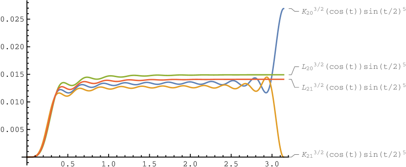
Figure 3: Plots of the functions $K_{20}^{\frac{3}{2}}(\cos\vartheta)(\sin\frac{\vartheta}{2})^{5}$, $K_{21}^{\frac{3}{2}}(\cos\vartheta)(\sin\frac{\vartheta}{2})^{5}$, $L_{20}^{\frac{3}{2}}(\cos\vartheta)(\sin\frac{\vartheta}{2})^{5}$, and $L_{21}^{\frac{3}{2}}(\cos\vartheta)(\sin\frac{\vartheta}{2})^{5}$. Again the parity phenomenon for the kernel $K$ is prominently visible.

Remark 5

Notice that the orders of magnitude in terms of $n$ and the powers of $\sin\frac{\vartheta}{2}$ are the same for $L_{n}^{\lambda}$ as for the kernel $K_{n}^{\lambda}$. This fact is illustrated by Figure 3. The coefficient of the asymptotic leading term of the estimate decays like $(2\lambda+1)(C/4)^{\lambda}$ for $L_{n}^{\lambda}$, whereas this coefficient decays like $(2\lambda+1)(1/2)^{\lambda}$ for $K_{n}^{\lambda}$.

References

(1)
Andrews, G. E., Askey, R., Roy, R.: Special functions, Encyclopedia of
Mathematics and its Applications, vol. 71, Cambridge University Press,
Cambridge (1999)
(2)
Berens, H., Butzer, P. L., Pawelke, S.: Limitierungsverfahren von
Reihen mehrdimensionaler Kugelfunktionen und deren
Saturationsverhalten, Publ. Res. Inst. Math. Sci. Ser. A
4, 201–268 (1968/1969)
(3)
E. Kogbetliantz, Recherches sur la sommabilité; des séries
ultra-sphériques par la méthode des moyennes arithmétiques, J.
Math. Pures Appl. 3, 107–188, (1924)
(4)
M. Reimer, A short proof of a result of Kogbetliantz on the positivity
of certain Cesàro means, Math. Z. 221(2), 189–192 (1996)