Evidence for spatially-correlated Gaia parallax errors in the Kepler field

Abstract

We present evidence for a spatially-dependent systematic error in the first data release of Gaia parallaxes based on comparisons to asteroseismic parallaxes in the Kepler field, and present a parametrized model of the angular dependence of these systematics. We report an error of $0.059^{+0.004}_{-0.004}$mas on scales of $0.3$deg, which decreases for larger scales to become $0.011^{+0.006}_{-0.004}$mas at $8$deg. This is consistent with the $\sim 2\%$ zeropoint offset for the whole sample discussed by Huber et al., and is compatible with the effect predicted by the Gaia team. Our results are robust to dust prescriptions and choices in temperature scales used to calculate asteroseismic parallaxes. We also do not find evidence for significant differences in the signal when using red clump versus red giant stars. Our approach allows us to quantify and map the correlations in an astrophysically interesting field, resulting in a parametrized model of the spatial systematics that can be used to construct a covariance matrix for any work that relies upon TGAS parallaxes.

1 Introduction

The Gaia mission is expected to provide positions, parallaxes, and proper motions for a billion objects, with precisions of $\sim 20$ micro-arcseconds ($\mu$as) for stars down to $15^{\mathrm{th}}$ magnitude (Gaia Collaboration et al., 2016a). Though the final data release is scheduled for 2022, positions, parallaxes, and proper motions for $2$ million stars common to Tycho-2 (Høg et al., 2000) and Gaia have been released as part of Data Release 1 (DR1) (Gaia Collaboration et al., 2016b). By using positions from Tycho-2 as priors on the astrometric solution, Michalik et al. (2015) demonstrated that sub-milliarcsecond accuracy could be achieved, resulting in the Tycho-Gaia Astrometric Solution (TGAS). Though the statistical errors may even be smaller than the $0.3$mas reported in DR1 (see Gould et al., 2016), systematic errors are expected to exist at the level of up to $0.3$mas (Lindegren et al., 2016). Various instrumental and modeling effects that may account for the systematic errors are explored in Lindegren et al. (2016), including the known chromaticity of the CCDs, inadequate temporal resolution of the satellite attitude model, and so-called ‘micro-clanks’ due to mechanical jitter.

In this work, we compute asteroseismic parallaxes for more than 1000 red giants in the $10^{\circ}\times 10^{\circ}$ Kepler field of view for comparison to TGAS parallaxes. Thanks to the order-of-magnitude better precision of asteroseismic parallaxes for red giants, and the high stellar density of the Kepler field, we are able to investigate the presence of correlated errors in TGAS parallaxes on degree and sub-degree scales in an effort to quantify the expected systematic spatial errors in TGAS parallax.

To date, other comparisons of the asteroseismic parallax scale to the TGAS parallax scale have considered global offsets — i.e., non–spatially-dependent differences. De Ridder et al. (2016), for instance, found good agreement between the two scales for a sample of 22 dwarfs and sub-dwarfs, but significant differences among 938 red giants. Huber et al. (in press) suggest that a global offset is partially mitigated when using a hotter temperature scale such as the infrared flux method temperature scale, and that radii inferred from TGAS parallaxes are consistent with asteroseismic radii to within $5\%$ between $0.8$–$8R_{\odot}$.

Compared to other parallax scales, the TGAS parallax scale exhibits a fractional offset. Davies et al. (2017), for example, attributed the red giant asteroseismic parallax offset from De Ridder et al. (2016) to errors in the TGAS parallax scale by comparing TGAS parallaxes to red clump distances. Their suggested correction agrees for $\varpi\gtrsim 1.6$ with that of Stassun & Torres (2016a), who compared TGAS parallaxes to parallaxes from eclipsing binaries. Huber et al. (in press) found that these offsets are too large, and can be partially attributed to a too cool temperature scale, based on a larger sample of stars spanning from the main sequence to the red giant branch. At larger distances, Sesar et al. (2017) found no evidence for a global offset when comparing to RR Lyrae parallaxes at a median parallax of $0.8$mas, and neither did Casertano et al. (2017) when looking at Cepheid parallaxes. And at the smallest distances, Jao et al. (2016) found evidence for a correction consistent with that of Stassun & Torres (2016a) (amounting to $\approx 0.2$mas in the sense that TGAS overestimates distances) when compared to trigonometric parallaxes for 612 dwarfs at distances of less than $100$pc.

To date, two studies independent of the Gaia team have mentioned possible spatial dependencies in TGAS parallax scales. Casertano et al. (2017) found mild evidence for spatially-correlated TGAS parallaxes at the level of $19\pm 34\mu$as on scales less than $10$deg using Cepheids, while Jao et al. (2016) reported a North-South ecliptic hemisphere difference in trigonometric and TGAS parallaxes. Despite the thorough investigation of the quantitative and qualitative existence of such systematic errors in Lindegren et al. (2016), the precise characterization of spatially-dependent systematics in terms of a functional form and/or a characteristic scale at which the $0.3$mas systematic error applies was not released for DR1. Our exercise, then, is to identify and to characterize any spatial correlation of parallax errors in Gaia DR1.

The structure of this paper is as follows: we describe the provenance of and basic calibrations of the observables used to compute asteroseismic parallax in §2. In §3, we detail how we compute asteroseismic parallaxes, treatment of statistical errors therein, and how we test for the presence of spatially-correlated offsets between asteroseismic TGAS parallaxes. We summarize our main findings in §4, discuss potential caveats to those findings in §5, and conclude in §6.

2 Data

Quantifying any systematic errors in Gaia parallaxes requires an independent and unbiased set of parallaxes to compare to the TGAS values. The Gaia team validated their parallaxes against Hipparcos parallaxes, which revealed the presence of systematic offsets (Lindegren et al., 2016). We attempt to present a complementary treatment of potential errors in the TGAS parallax scale for two main reasons. First, the Hipparcos parallaxes themselves have spatially-correlated errors (see references in §5), which limits their usefulness when used as a validation set. More critically, a detailed model of the spatial correlations of TGAS parallax errors has not yet been published, which would be crucial to proper treatment of errors in work using TGAS between now and April 2018, when the next Gaia data release is scheduled.

Our validation set consists of parallaxes of red giants in the Kepler field of view that have spectroscopic metallicities and asteroseismic data, which permits us to infer effective temperature, radii, and, by extension, luminosities. Adding reddening and bolometric flux information then yields distances and hence parallaxes. The resulting asteroseismic parallaxes have statistical errors an order-of-magnitude smaller than those in TGAS, and hence permit a strong test of spatially-correlated offsets in TGAS versus asteroseismic parallax scales.

Our sample consists of over 1000 red giants spread across the $\sim 100$ sq. deg. Kepler field of view, which means that we can probe systematic parallax offsets on scales less than a degree. This is the scale where Lindegren et al. (2016) indicate systematic errors in the TGAS parallaxes are expected to be the largest.

The basis for our sample are TGAS stars that are also listed as asteroseismic giants in the APOGEE-Kepler Asteroseismic Science Consortium catalogue (APOKASC; Pinsonneault et al., 2014), which combines infrared spectroscopic data from Data Release 13 of the The Apache Point Observatory Galactic Evolution Experiment (APOGEE) (Zasowski et al., 2013; Majewski et al., 2015) with asteroseismic data from the Kepler mission (Borucki et al., 2010). We now discuss the provenance of spectroscopic metallicities, asteroseismic parameters, reddenings, and photometry in turn.

APOGEE temperatures, $T_{\mathrm{eff,APOGEE}}$, and metallicities, $\mathrm{[Fe/H]}$, are taken from the Thirteenth Data Release of the Sloan Digital Sky Survey (DR13; SDSS; SDSS Collaboration et al., 2016), and are corrected according to the metallicity-dependent term recommended in the DR13 documentation. Global asteroseismic parameters $\nu_{\mathrm{max}}$ and $\Delta\nu$ — which may be mapped into stellar radii — were adopted from the SYD pipeline (Huber et al., 2009) values in version 3.6.5 of the APOKASC catalogue (Pinsonneault et al., in prep.).

Because there is evidence that asteroseismic radii have evolutionary state–dependent systematics (e.g., Miglio et al., 2012), we divide the TGAS-APOKASC giant sample into red giant branch (RGB) and red clump (RC) sub-samples, to assess any differences in TGAS-asteroseismic parallax offsets as a function of evolutionary state. Evolutionary state information is compiled from the asteroseismic classifications of Stello et al. (2013) or Mosser et al. (2014) (Elsworth et al., in prep.).

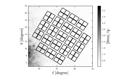
Extinction corrections (described in §3.1) are made using the three-dimensional dust map of Green et al. (2015), as implemented in mwdust (Bovy et al., 2016). The $A_{V}$ extinction for the Kepler field of view is shown in Figure 1.

We opt to calculate an effective temperature and bolometric flux using the InfraRed Flux Method (IRFM), as implemented in González Hernández & Bonifacio (2009), which was used to set the APOGEE effective temperature scale. For this purpose, we use near-infrared photometry in the $J$, $H$, and $K_{\mathrm{s}}$ bands from the Two Micron All Sky Survey (2MASS; Skrutskie et al., 2006). Visual photometry is also required, which we derive from SDSS $g$ and $r$ photometry. We choose to convert these magnitudes to Johnson $B$ and $V$ according to Lupton (2005) rather than use Tycho $B$ and $V$. In doing so, the resulting visual photometry has less scatter than Tycho $B$ and $V$. Furthermore, the $griz$ photometry from the Kepler Input Catalogue (KIC; Brown et al., 2011), as re-calibrated to be on the SDSS scale by Pinsonneault et al. (2012), is consistent with the 2MASS infrared photometry temperature scale for cool stars (see Pinsonneault et al., 2012).

The requirement that our sample of stars have $grJHK_{\mathrm{s}}$, $\nu_{\mathrm{max}}$, $\Delta\nu$, $T_{\mathrm{eff,APOGEE}}$, $\mathrm{[Fe/H]}$, RGB or RC evolutionary state classifications, and Gaia DR1 parallaxes ($\varpi_{\mathrm{TGAS}}$) yields a base sample of 1592 giants.

2.1 Quality cuts

We omit stars known to be members of NGC6791 and NGC6819, as giants residing in these clusters could bias measurements of spatially-correlated quantities.

Comparisons by Gould et al. (2016) of TGAS parallaxes to RR Lyrae parallaxes indicated that DR1 TGAS parallax statistical errors are inflated by $\sim 30\%$. Because the calculation of a spatially-correlated TGAS-asteroseismic parallax offset will be more robust with a proper treatment of the statistical errors, we modify those for the TGAS parallaxes according to their prescription. Reducing statistical errors in this way does not introduce a spatially-correlated, systematic offset of the sort we present in this work.

Finally, TGAS parallaxes are required to have a signal-to-noise ratio greater than $1.6$ (see §3.3).

The above quality cuts yield a total of 1392 giants, which comprise the final TGAS-APOKASC sample used in the following.

Figure 1: We use a three-dimensional dust map from Green et al. (2015), as implemented in mwdust (Bovy et al., 2016). Shown here is $A_{V}$ in the region of the Kepler field of view, in Galactic coordinates. Choosing to include or not the higher extinction region $\ell\lesssim 73^{\circ}$ does not eliminate spatially-correlated offsets between asteroseismic and TGAS parallaxes.

3 Methods

3.1 Asteroseismic parallax

Estimating errors in TGAS parallaxes requires an independent distance measure. Apart from the moving group or parallax methods, distance estimates of stars will require an estimate of stellar luminosity and its bolometric flux. For our purposes, we use asteroseismology to determine stellar luminosity and the infrared flux method to determine a bolometric flux, which are combined to yield a parallax/distance. As the following overview will show, asteroseismology effectively provides a radius, which in combination with an effective temperature of the star, will determine its luminosity via the Stefan-Boltzmann equation; combined with the bolometric flux of the star, one can determine its distance.

In this work, we estimate stellar radius by way of two complementary scaling relations involving two different asteroseismic observables: $\nu_{\mathrm{max}}$ (roughly the frequency at which the largest-amplitude acoustic modes occur) and $\Delta\nu$, the separation between acoustic modes of the same spherical harmonic degree, $\ell$, but differing by one radial order number, $n$.

It is well-established (see, e.g., Tassoul, 1980; Christensen-Dalsgaard, 1993) that $\Delta\nu$ is related to the mean density of a star via a scaling relation, assuming homologous behavior between the Sun and a given star, of the form

$$\frac{\Delta\nu}{\Delta\nu_{\odot}}\approx\sqrt{\frac{M/M_{\odot}}{(R/R_{\odot})^{3}}}.$$ (1)

Similarly, the frequency of maximum acoustic power, $\nu_{\mathrm{max}}$, has been found to scale as the acoustic cutoff frequency (Brown et al., 1991; Kjeldsen & Bedding, 1995; Chaplin et al., 2008), i.e., as

$$\frac{\nu_{\mathrm{max}}}{\nu_{\mathrm{max,}\odot}}\approx\frac{M/M_{\odot}}{(R/R_{\odot})^{2}\sqrt{(T_{\mathrm{eff}}/T_{\mathrm{eff,}\odot})}}.$$ (2)

We can combine these two relations to yield an estimate of the radius, $R$, of the star:

$$(R/R_{\odot})\approx(\nu_{\mathrm{max}}/\nu_{\mathrm{max,}\odot})(\Delta\nu/\Delta\nu_{\odot})^{-2}(T_{\mathrm{eff}}/T_{\mathrm{eff,}\odot})^{1/2}.$$ (3)

With a temperature and the radius, we can compute a luminosity and thus a luminosity distance/parallax, provided we know the bolometric flux, $F_{\mathrm{bol}}$:

$$\varpi_{\mathrm{astero}}=\frac{\sqrt{F_{\mathrm{bol}}}}{R\sqrt{\sigma_{\mathrm{SB}}}T_{\mathrm{eff}}^{2}},$$ (4)

with $\sigma_{\mathrm{SB}}$ being the Stefan-Boltzmann constant. We adopt solar values consistent with those of Huber et al. (2009): $\nu_{\mathrm{max,}\odot}=3090\mu\mathrm{Hz}$; $\Delta\nu_{\odot}=135.1\mu\mathrm{Hz}$; $T_{\mathrm{eff,}\odot}=5777$K; and $\log~{}g_{\odot}=4.438$ (Mamajek et al., 2015).

Figure 2: APOGEE and IRFM temperature scales show a systematic offset that is temperature-dependent. We find that $T_{\mathrm{eff,IRFM}}$ results in parallaxes more consistent with those from TGAS, and use this temperature scale instead of $T_{\mathrm{eff,APOGEE}}$ throughout the paper. Grey dashed lines show one-to-one relations. Median errors on both quantities are shown by the error bar in the top panel. The bottom panel shows a binned median of the temperature difference (grey curve), with grey error bars representing the standard deviation of the difference within each bin and red error bars representing the statistical error on the median within each bin. The IRFM temperature is hotter than APOGEE spectroscopic temperatures by $65\pm 13$K, on average.

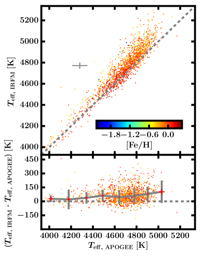
With a radius from asteroseismology, we turn to the bolometric flux and effective temperature, which we infer from the infrared flux method (IRFM) using $BVJHK_{\mathrm{s}}$ photometry, according to González Hernández & Bonifacio (2009). Calculating an effective temperature using the IRFM allows us to self-consistently estimate the reddening (and hence extinction) to each star, which is necessary to achieve a correct distance measure. The basic approach is to simultaneously fit a star’s spectral energy distribution from the optical to the infrared, taking advantage of the insensitivity of infrared stellar emission on effective temperature. First, the observed infrared flux is compared to the infrared flux for a model atmosphere, yielding an angular diameter. Next, a bolometric flux is computed by combining other photometric information (e.g., optical) with infrared photometry, based on an assumed stellar atmosphere model. Finally, a temperature is determined by using the previously computed bolometric flux and angular diameter. The bolometric flux and temperature results converge iteratively. Since the IRFM requires stellar atmosphere lookups as a function of $\mathrm{[Fe/H]}$, $\log~{}g$, and $T_{\mathrm{eff}}$, we implement the IRFM using guesses for these quantities from APOGEE. For the whole process, we assume a fixed metallicity from APOGEE, $\mathrm{[Fe/H]}$. Our initial guess for $T_{\mathrm{eff}}$ is $T_{\mathrm{eff,APOGEE}}$; our initial guess for $\log~{}g$ is calculated from Equation 2 using $T_{\mathrm{eff,APOGEE}}$. An IRFM temperature and bolometric flux are then computed iteratively, as described in González Hernández & Bonifacio (2009). The resulting IRFM temperature, $T_{\mathrm{eff,IRFM}}$, is used to compute a new $\log~{}g$, and the bolometric flux is used via Equation 4 to compute an asteroseismic distance/parallax, $\varpi_{\mathrm{astero}}$. An extinction for each band is then computed using the three-dimensional dust map of Green et al. (2015) using mwdust (Bovy et al., 2016), with which we correct the $JHK_{\mathrm{s}}$ photometry, yielding dust–de-extincted $J_{0}$, $H_{0}$, and $K_{\mathrm{s,\ 0}}$. $B_{0}$ and $V_{0}$ are computed by transforming corrected $g$ and $r$ magnitudes, $g_{0}$ and $r_{0}$. This corrected photometry is then used in subsequent iterations to compute the bolometric flux and temperature, and the process is repeated until convergence in the asteroseismic parallax. We compute uncertainties on the derived quantities $B_{0}$, $V_{0}$, $J_{0}$, $H_{0}$, $K_{\mathrm{s,\ 0}}$, $A_{V}$, $\log~{}g$, $T_{\mathrm{eff,IRFM}}$, and $\varpi_{\mathrm{astero}}$ by repeating the iterative process, perturbing the observable quantities $g$, $r$, $J$, $H$, $K_{\mathrm{s}}$, $\nu_{\mathrm{max}}$, $\Delta\nu$, $T_{\mathrm{eff,APOGEE}}$, and $\mathrm{[Fe/H]}$ based on their statistical errors , and imposing a minimum uncertainty of $0.08$mag for $A_{V}$ to account for variations in $R_{V}$ within the Kepler field and for line-of-sight variations below the resolution of the Green et al. (2015) dust map ($\sim 0.05$deg). Resulting IRFM temperatures are shown in Figure 2. When compared to APOGEE spectroscopic temperatures, the IRFM temperatures are on average $\sim 70$K hotter. As we have found in Huber et al. (in press), the IRFM temperature scale results in a smaller global offset between asteroseismic and TGAS parallaxes than when using, e.g., spectroscopic temperatures from APOGEE.

Figure 3: The absolute magnitude in these Hertzsprung-Russell diagrams for the TGAS-ASPOKASC sample are computed via the IRFM (see text), and either an asteroseismic parallax (left) or a TGAS parallax (right). Median error bars are shown in black. Red clump stars are shown in red and red giant branch stars in blue.

Figure 4: A two-dimensional histogram of statistical errors on parallax versus parallax for asteroseismic parallaxes derived in this work (left) and for TGAS parallaxes (right). The former are an order-of-magnitude more precise than the latter, which makes the TGAS-APOKASC sample in this work a powerful calibrator for investigating systematic errors in TGAS parallaxes.

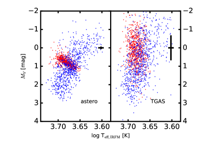
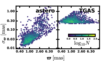
For purposes of illustration, Hertzsprung-Russell diagrams are constructed in Figure 3 from asteroseismic and TGAS parallaxes in combination with de-extincted V-band magnitudes, $V_{0}$. We employ an exponentially decreasing space density prior with a scale length of $1.35$kpc (Bailer-Jones, 2015; Astraatmadja & Bailer-Jones, 2016) for the conversion of parallax to distance. The red clump is particularly sharp using asteroseismic parallaxes compared to the spread of red clump luminosities assuming TGAS parallaxes. Figure 4 demonstrates the relative precision of asteroseismic and TGAS parallaxes as a two-dimensional histogram of statistical parallax error versus parallax for the TGAS-APOKASC giant sample; the median uncertainty for asteroseismic parallaxes is $0.03$mas and the median uncertainty for TGAS parallaxes is $0.3$mas. Clearly, the error budget in the comparisons between the scales is dominated by TGAS parallax uncertainties.

Figure 5: Comparison of our $A_{V}$ to the KIC estimates (Brown et al., 2011), $A_{\mathrm{V,\ KIC}}$. Grey dashed lines show one-to-one relations. The grey error bar in the top panel indicates the median uncertainty on $A_{V}$ for our derived extinctions. Note that uncertainties on extinctions are not reported for the KIC, and that a minimum uncertainty on our derived extinctions of 0.08mag is imposed. The black line is the relation between visual extinctions derived in Rodrigues et al. (2014) and KIC extinctions. The bottom panel shows a binned median, with grey error bars representing the scatter in each bin.

3.2 Extinction

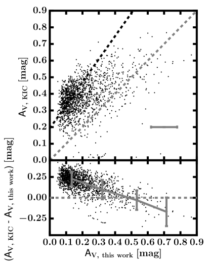
Extinction values are computed as a result of the iterative procedure described in §3.1, which we have compared to extinctions from the Kepler Input Catalogue (KIC; Brown et al., 2011). Previous studies suggest that the KIC extinctions are over-estimated (Rodrigues et al., 2014; Zasowski et al., 2015), and we also find that our extinction values are smaller than those in the KIC. Figure 5 shows that the offset between our derived extinctions and KIC extinctions is comparable to to the offset when checking against Bayesian extinction estimates of APOKASC giants in Rodrigues et al. (2014), who found $A_{\mathrm{V}}=(0.721\pm 0.015)A_{\mathrm{V,\ KIC}}-(0.139\pm 0.007)$. This relation is plotted as a black dashed line on top of our extinctions. Our extinctions based on Green et al. (2015) dust maps also compare well to the extinctions derived from grid-based modeling in Huber et al. (in press). mwdust offers several dust maps, and our result does not significantly change if using the Green et al. (2015) map or a combination of individual maps from Marshall et al. (2006), Green et al. (2015), and Drimmel et al. (2003), as synthesized by Bovy et al. (2016).

(a)

(b)

Figure 6: Comparison of TGAS and asteroseismic parallax scales before ( left) and after ( right) a signal-to-noise ratio cut of $\mathrm{SNR}>1.6$. Median uncertainties are shown as the grey error bars in the top axes. Grey dashed lines show one-to-one relations. The bottom axes show running medians of the fractional parallax differences (grey curves), with grey error bars representing the standard deviation of the difference within each bin and red error bars representing the statistical error on the median within each bin.

3.3 Final TGAS-APOKASC sample

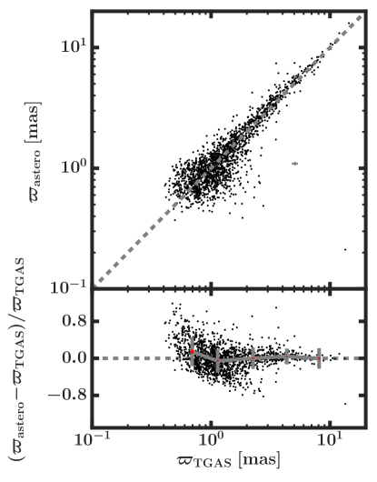
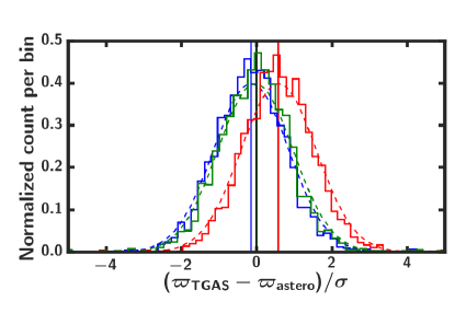
In Figure 6, we show a direct star-by-star comparison of the two parallax scales. It is evident that at smaller $\varpi$, there is a systematic offset between the two scales. This offset is expected from comparing a precise asteroseismic parallax sample to a much less precise sample of TGAS parallaxes: the large fractional errors on TGAS parallax will tend to scatter to low parallax. We can mitigate the offset by applying a signal-to-noise cut such that the median of the difference between the two parallaxes is zero, to within the error on the median. We show the original distribution and the distribution of the parallax difference after a signal-to-noise cut of $\mathrm{SNR}>1.6$ in Figure 7. A potential zeropoint offset in asteroseismic and TGAS parallax scales is discussed in §5.5 (see also Huber et al., in press). We use the high signal-to-noise sample for the rest of the analysis (TGAS-APOKASC sample), which numbers 1392.

Figure 7: The distribution of TGAS and asteroseismic parallax differences, in the sense of TGAS - asteroseismic, normalized by the statistical error on the difference, assuming normality. In blue is the base sample of 1592 stars before a signal-to-noise ratio cut. In red, a zeropoint correction is applied to the base sample, as recommended in Stassun & Torres (2016a). In green is the final TGAS-APOKASC sample of 1392 stars, which differs from the base sample by a signal-to-noise cut of $\mathrm{SNR}>1.6$ such that the median of the resulting distribution is equal to zero, to within the error on the median (a parallax difference of zero is shown as black vertical line).

4 Results

4.1 Spatially-correlated offsets in asteroseismic and TGAS parallaxes

Figure 8: The Pearson correlation coefficient, in bins of angular separation on the sky, which will be positive for correlated TGAS-asteroseismic parallax offsets, zero in the absence of correlated offsets, and negative for anti-correlated offsets. Error bars include a bootstrap and ‘systematic’ error; the black line indicates the best-fitting model of the form in Equation 7; the green band indicates the $68\%$ confidence interval of the recovered binned Pearson correlation coefficient, as computed from a mock catalogue of TGAS parallaxes assuming asteroseismic parallaxes as the true value and spatial correlations according to the black line. Refer to §4.2 for details.

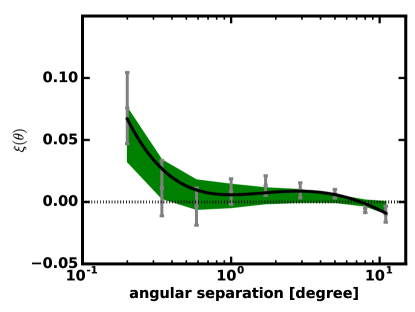
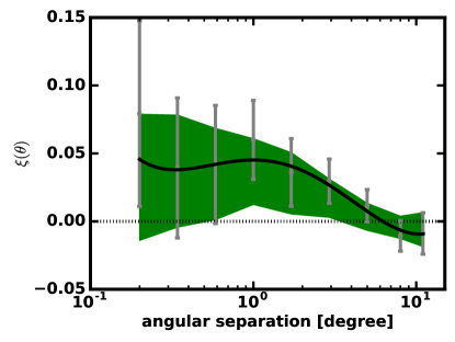
Figure 8 shows our main result, which is a measure of the spatial correlation of the difference in the TGAS and asteroseismic parallax scales for all 1392 giants in the TGAS-APOKASC sample. Below, we first discuss the choice of a binned Pearson correlation coefficient as a metric for the spatially-correlated parallax difference and how it is calculated, and then present model fits to the observed signal.

4.2 Quantification using a binned Pearson correlation coefficient

Our measure of the parallax offset spatial correlation is a binned Pearson correlation coefficient,

$$\xi(\theta)\equiv\frac{\sum_{i\neq j}(\varpi_{\mathrm{TGAS,i}}-\varpi_{\mathrm{astero,i}})_{\theta}(\varpi_{\mathrm{TGAS,j}}-\varpi_{\mathrm{astero,j}})_{\theta}}{\sqrt{((\varpi_{\mathrm{TGAS,i}}-\varpi_{\mathrm{astero,i}})^{2})_{\theta}((\varpi_{\mathrm{TGAS,j}}-\varpi_{\mathrm{astero,j}})^{2})_{\theta}}},$$ (5)

where $i$ and $j$ denote stars that are separated by an angle, $\theta^{\prime}$, such that $\theta-\Delta\theta/2<\theta^{\prime}<\theta+\Delta\theta/2$ for a given angular bin size $\Delta\theta$. Equation 5 describes a Pearson correlation coefficient computed in bins of angular separation. A value of $-1$ indicates that $\varpi_{\mathrm{TGAS}}$ and $\varpi_{\mathrm{astero}}$ are perfectly anti-correlated at that separation; a value of $+1$ indicates that they are perfectly correlated; a value of $0$ indicates they are not correlated. In the absence of spatial errors, then, we would expect a null signal of zero at all angular separations. For errors that increase at small separations, there would be a rise in $\xi(\theta)$ with decreasing $\theta$. A zeropoint error would result in a flat, positive $\xi(\theta)$ for all $\theta$.

We compute error bars in the binned Pearson correlation coefficient via bootstrapping (Loh, 2008). Briefly, the sample of objects were divided into $N$ spatial regions, which were then sampled with replacement (meaning the same region could be used multiple times in a single bootstrap sample) $N$ times to create a bootstrap sample; we divided the sample into spatial regions according to their Kepler module. For $B$ such samples, the $100(1-\alpha)\%$ confidence intervals on each point in the binned Pearson correlation coefficient were computed according to the bootstrap confidence interval (Davison & Hinkley, 1997):

$$\left[2\hat{K}-K_{(B+1)(1-\alpha/2)},2\hat{K}-K_{(B+1)\alpha/2}\right],$$

where $K_{\mathrm{A}}$ is the A^th-ranked statistic (the binned Pearson correlation coefficient, $K=\xi$, in this case) computed from a bootstrap sample and $\hat{K}$ is the statistic computed using all the data.

In order to better characterize the errors on the statistic, we create mock TGAS stellar catalogues, whose positions are the same as those in the data, but whose parallaxes are drawn from the asteroseismic parallaxes, and injected with spatial correlations according to Equation 7, assuming Gaussian statistics, with best-fitting values from Table 1 (see §4.3). These fake TGAS parallaxes are then used to compute the binned Pearson correlation coefficient according to Equation 5, and the resulting distribution of values at each angular bin are used to compute a $68\%$ confidence interval — a ‘systematic’ error — for the statistic. Note that our mock catalogue generation assumes Gaussianity in the distribution of TGAS-asteroseismic parallax difference, which we think is reasonable given the evident Gaussianity of the distribution shown in Figure 7. This ‘systematic’ error is shown as a green band in Figure 8.

We also provide alternate representations of the TGAS-asteroseismic parallax offset in Figures 17 & 18. Both alternate representations indicate a spatial dependence in the offset, in agreement with the binned Pearson correlation coefficient. See the Appendix for details on how these alternate measures are computed.

(a)

(b)

(c)

Figure 9: The distribution of TGAS and asteroseismic parallax differences, in the sense of TGAS-asteroseismic, normalized by the statistical error on the difference, $\sigma\equiv\sqrt{\sigma_{\varpi_{\mathrm{TGAS}}}^{2}+\sigma_{\varpi_{\mathrm{astero}}}^{2}}$, as a function of position on the sky. The smoothed field is calculated by convolving the observed data with a Gaussian filter of standard deviation $0.2$deg. Panel a shows the signal in the TGAS-APOKASC sample; panel b shows a model with no spatial correlation; panel c shows the best-fitting model of panel a, with random spatial phase (see §4.3).

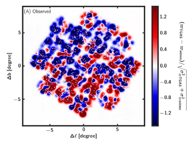
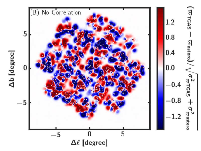
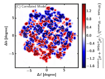
For visualization purposes, a spatial map of the TGAS-asteroseismic parallax offset is plotted in Figure 9a. Each point represents a star in the TGAS-APOKASC sample and is colored by $(\varpi_{\mathrm{TGAS}}-\varpi_{\mathrm{astero}})/\sigma$, where $\sigma$ is the quadrature sum of the statistical errors from $\varpi_{\mathrm{TGAS}}$ and $\varpi_{\mathrm{astero}}$. A smoothed version of the data is calculated by convolving these values by a Gaussian with $0.2$deg standard deviation. For comparison, a map of parallax offset with no spatial correlation is simulated in Figure 9b. Whereas there is visible structure shown in the observed TGAS-asteroseismic parallax differences of Figure 9a, there are no such correlated hot or cold spots in Figure 9b. For comparison, a map injected with spatial correlations according to Equation 7, assuming Gaussian statistics, with best-fitting values from Table 1, is shown in Figure 9c. The spatial correlation model of Figure 9c qualitatively reproduces the patchwork structure seen in the data ( Figure 9a).

4.3 Fitting models to the observed spatially-correlated offset

We fit an analytic form to the observed spatial correlation in order to determine a characteristic scale at which the systematic error is important. We consider two models — one with exponential spatial scale dependence, as might be expected from the Gaia scanning strategy, in which characteristic spatial scales could be strongly imprinted in the data. The first model we fit to the binned Pearson correlation coefficient is a purely exponential model of the form

$$\xi(\theta)=\rho_{\mathrm{max}}\exp{\left[-\theta/\theta_{1/2}\ln 2\right]}+C.$$ (6)

Note that in the above expression, $\rho_{\mathrm{max}}$ is an overall amplitude to the spatially-varying component of $\xi$, and that $\theta_{1/2}$ represents the angular scale at which spatial correlations are half of what they are at the smallest scales.

We also fit a polynomial of the form

$$\xi(\theta)=A+B\log\theta+C(\log\theta)^{2}+D(\log\theta)^{3}+E(\log\theta)^{4}.$$ (7)

We computed best-fitting parameters and their associated uncertainties by fitting with the PYTHON MCMC routine of emcee (Foreman-Mackey et al., 2013) with a covariance matrix calculated from the bootstrap sample, whose diagonal is added in quadrature with the ‘systematic’ error, described above.

In Table 1, we provide the resulting best-fitting parameters for the spatially-correlated parallax offset models. We also provide best-fitting parameters for the RGB and RC sub-samples separately (see §5.2). According to the Akaike Information Criterion (Akaike, 1973), $AIC\equiv 2k-\ln\mathcal{L}$, where $k$ is the number of degrees of freedom and $\ln\mathcal{L}=-0.5\chi^{2}$ is the log-likelihood, Equation 6 is preferred in the fits to binned Pearson correlation coefficient for RGBs and RCs, but Equation 7 is preferred for the combined TGAS-APOKASC sample. We take preference of model 1 over model 2 to be $AIC_{\mathrm{model1}}-AIC_{\mathrm{model2}}<-2$. We refer to the best-fitting model as Equation 7, and recommend the fits to this polynomial model for characterizing covariance matrices. For completeness, we have also compared preference for both models to a null model of zero at all angular scales, finding that the null model is never preferred.

Systematic offsets at a given angular scale, $\theta$, $\sigma_{\mathrm{sys}}(\theta)$, are also reported in Table 1. They are calculated according to

$$\sigma_{\mathrm{sys}}(\theta)=\sqrt{|\xi(\theta)|\sigma^{2}},$$ (8)

where $\sigma\equiv\sqrt{\sigma_{\varpi_{\mathrm{TGAS}}}^{2}+\sigma_{\varpi_{\mathrm{astero}}}^{2}}$. Confidence intervals on $\sigma_{\mathrm{sys}}$ are computed using a covariance matrix built from the MCMC chains from model-fitting (see above), according to which a representative distribution of model parameters is drawn, and for which a resulting distribution of possible $\sigma_{\mathrm{sys}}$ is computed. Note that the sense of this systematic offset between the two parallax scales is not indicated, as it will vary as a function of absolute position on the sky. One can see, for instance, the regions where the sign change of the offset switches in Figure 9. Rather, signs on this systematic offset provided in Table 1 indicate correlation (positive) versus anti-correlation (negative).

Our best-fitting polynomial model using the entire TGAS-APOKASC sample yields parallax offsets at the smallest separations of $0.059^{+0.004}_{-0.004}$mas and $0.011^{+0.006}_{-0.004}$mas at spacial scales of $\theta\approx 0.3$deg and $\theta\approx 8$deg, respectively.

Table 1: Fits to models of the spatially-correlated TGAS-asteroseismic parallax offset

sample	model	$\rho_{\mathrm{max}}/A$	$\theta_{1/2}/B$	$C$	$D$	$E$	$\chi^{2}/dof$	$\sigma_{\mathrm{{sys}}}(\theta=\theta_{1/2})$	$\sigma_{\mathrm{{sys}}}(\theta=0.0^{\circ})$	$\sigma_{\mathrm{{sys}}}(\theta=0.3^{\circ})$	$\sigma_{\mathrm{{sys}}}(\theta=1.0^{\circ})$	$\sigma_{\mathrm{{sys}}}(\theta=8.0^{\circ})$
ALL	$Eq.\ref{eq:model1}^{*}$	$0.059^{+0.045}_{-0.045}$	$0.110^{+0.040\circ}_{-0.040}$	$0.0032^{+0.0005}_{-0.0005}$			7.287	$0.050^{+0.016}_{-0.022}$mas	$0.078^{+0.025}_{-0.037}$mas	$0.030^{+0.010}_{-0.011}$mas	$0.018^{+0.001}_{-0.002}$mas	$0.017^{+0.001}_{-0.001}$mas
ALL	$Eq.\ref{eq:model2}^{*+}$	$0.006^{+0.002}_{-0.002}$	$-0.022^{+0.575\circ}_{-0.575}$	$0.009^{+0.001}_{-0.001}$	$-0.007^{+0.001}_{-0.001}$	$0.0010^{+0.0003}_{-0.0003}$	4.850	$\cdots$	$\cdots$	$0.059^{+0.004}_{-0.004}$mas	$0.024^{+0.004}_{-0.005}$mas	$-0.011^{+0.006}_{-0.004}$mas
RC	$Eq.\ref{eq:model1}^{*}$	$0.085^{+0.019}_{-0.019}$	$4.970^{+2.035\circ}_{-2.035}$	$-0.0310^{+0.0172}_{-0.0172}$			0.976	$0.031^{+0.006}_{-0.009}$mas	$0.071^{+0.006}_{-0.007}$mas	$0.068^{+0.007}_{-0.007}$mas	$0.062^{+0.006}_{-0.006}$mas	$-0.017^{+0.031}_{-0.011}$mas
RC	$Eq.\ref{eq:model2}^{*}$	$0.045^{+0.008}_{-0.008}$	$-0.025^{+0.583\circ}_{-0.583}$	$-0.014^{+0.006}_{-0.006}$	$-0.005^{+0.004}_{-0.004}$	$0.0028^{+0.0011}_{-0.0011}$	1.215	$\cdots$	$\cdots$	$0.058^{+0.011}_{-0.014}$mas	$0.065^{+0.005}_{-0.006}$mas	$-0.025^{+0.011}_{-0.006}$mas
RGB	$Eq.\ref{eq:model1}^{*}$	$0.104^{+0.027}_{-0.027}$	$7.590^{+1.793\circ}_{-1.793}$	$-0.0367^{+0.0206}_{-0.0206}$			0.230	$0.037^{+0.009}_{-0.013}$mas	$0.078^{+0.009}_{-0.009}$mas	$0.078^{+0.008}_{-0.010}$mas	$0.073^{+0.009}_{-0.010}$mas	$0.035^{+0.010}_{-0.015}$mas
RGB	$Eq.\ref{eq:model2}^{*}$	$0.072^{+0.018}_{-0.018}$	$-0.036^{+0.576\circ}_{-0.576}$	$-0.005^{+0.004}_{-0.004}$	$-0.009^{+0.004}_{-0.004}$	$0.0027^{+0.0014}_{-0.0014}$	0.044	$\cdots$	$\cdots$	$0.091^{+0.013}_{-0.015}$mas	$0.082^{+0.010}_{-0.011}$mas	$0.043^{+0.011}_{-0.014}$mas

Note. — Best-fitting parameters for Equations 6 & 7 for the spatially-correlated TGAS-asteroseismic parallax offset, with $68\%$ confidence interval errors. A positive (negative) value in the last five columns indicates the systematic offset is a positive correlation (an anti-correlation). An asterisk indicates preference of the model over a null signal based on the AIC criterion (see text). A plus sign indicates that the model of Equation 7 is preferred over the model of Equation 6 according to the AIC criterion.

Table 2: Spatial correlation in observables

observable	model	$\rho_{\mathrm{max}}$	$\theta_{1/2}$	$C$	$\chi^{2}/dof$	$\sigma_{\mathrm{{sys}}}(\theta=\theta_{1/2})$	$\sigma_{\mathrm{{sys}}}(\theta=0.0^{\circ})$	$\sigma_{\mathrm{{sys}}}(\theta=0.3^{\circ})$	$\sigma_{\mathrm{{sys}}}(\theta=1.0^{\circ})$	$\sigma_{\mathrm{{sys}}}(\theta=8.0^{\circ})$
$\nu_{\mathrm{max}}$	$Eq.\ref{eq:model1}^{*}$	$-0.004^{+0.010}_{-0.010}$	$6.085^{+2.628\circ}_{-2.628}$	$0.0011^{+0.0011}_{-0.0011}$	4.160	$-0.026^{+0.081}_{-0.049}$$\mu$Hz	$-0.046^{+0.126}_{-0.057}$$\mu$Hz	$-0.050^{+0.131}_{-0.053}$$\mu$Hz	$-0.039^{+0.115}_{-0.056}$$\mu$Hz	$-0.022^{+0.072}_{-0.042}$$\mu$Hz
$\Delta\nu$	$Eq.\ref{eq:model1}^{*}$	$-0.0036^{+0.0027}_{-0.0027}$	$5.8721^{+2.7097\circ}_{-2.7097}$	$0.0009^{+0.0011}_{-0.0011}$	4.6685	$-0.0008^{+0.0012}_{-0.0005}$$\mu$Hz	$-0.0015^{+0.0010}_{-0.0006}$$\mu$Hz	$-0.0014^{+0.0010}_{-0.0005}$$\mu$Hz	$-0.0013^{+0.0009}_{-0.0005}$$\mu$Hz	$-0.0007^{+0.0013}_{-0.0004}$$\mu$Hz
$T_{\mathrm{eff,IRFM}}$	$Eq.\ref{eq:model1}^{*}$	$0.007^{+0.021}_{-0.021}$	$0.845^{+3.170\circ}_{-3.170}$	$-0.0011^{+0.0013}_{-0.0013}$	1.445	$1.655^{+3.782}_{-5.467}$K	$2.358^{+3.013}_{-6.215}$K	$2.349^{+3.066}_{-5.968}$K	$1.787^{+4.162}_{-5.457}$K	$-0.815^{+15.744}_{-1.744}$K
$A_{V}$	$Eq.\ref{eq:model1}^{*}$	$0.923^{+0.057}_{-0.057}$	$4.805^{+0.516\circ}_{-0.516}$	$-0.3844^{+0.0546}_{-0.0546}$	0.920	$0.022^{+0.001}_{-0.001}$mag	$0.059^{+0.001}_{-0.001}$mag	$0.057^{+0.001}_{-0.001}$mag	$0.051^{+0.001}_{-0.001}$mag	$-0.024^{+0.001}_{-0.001}$mag
$\mathrm{[Fe/H]}$	$Eq.\ref{eq:model1}^{*}$	$0.025^{+0.005}_{-0.005}$	$8.144^{+1.581\circ}_{-1.581}$	$-0.0152^{+0.0042}_{-0.0042}$	1.529	$-0.0014^{+0.0002}_{-0.0001}$	$0.0025^{+0.0002}_{-0.0003}$	$0.0024^{+0.0002}_{-0.0003}$	$0.0022^{+0.0002}_{-0.0002}$	$-0.0013^{+0.0002}_{-0.0001}$
$J$	$Eq.\ref{eq:model1}^{*}$	$0.002^{+0.014}_{-0.014}$	$2.996^{+3.412\circ}_{-3.412}$	$-0.0006^{+0.0012}_{-0.0012}$	5.029	$-0.0003^{+0.0027}_{-0.0017}$mag	$0.0007^{+0.0017}_{-0.0031}$mag	$0.0006^{+0.0020}_{-0.0029}$mag	$0.0005^{+0.0021}_{-0.0026}$mag	$-0.0004^{+0.0034}_{-0.0010}$mag
$H$	$Eq.\ref{eq:model1}^{*}$	$0.008^{+0.017}_{-0.017}$	$0.636^{+3.311\circ}_{-3.311}$	$-0.0009^{+0.0014}_{-0.0014}$	2.299	$0.0015^{+0.0020}_{-0.0034}$mag	$0.0017^{+0.0014}_{-0.0036}$mag	$0.0015^{+0.0018}_{-0.0037}$mag	$0.0014^{+0.0025}_{-0.0035}$mag	$-0.0001^{+0.0109}_{-0.0011}$mag
$K_{\mathrm{s}}$	$Eq.\ref{eq:model1}$	$0.008^{+0.014}_{-0.014}$	$2.480^{+3.351\circ}_{-3.351}$	$-0.0013^{+0.0020}_{-0.0020}$	15.329	$0.0007^{+0.0028}_{-0.0021}$mag	$0.0015^{+0.0010}_{-0.0030}$mag	$0.0014^{+0.0013}_{-0.0029}$mag	$0.0011^{+0.0014}_{-0.0025}$mag	$-0.0002^{+0.0066}_{-0.0010}$mag
$g$	$Eq.\ref{eq:model1}^{*}$	$-0.008^{+0.002}_{-0.002}$	$3.049^{+2.163\circ}_{-2.163}$	$0.0017^{+0.0016}_{-0.0016}$	4.763	$-0.0005^{+0.0001}_{-0.0001}$mag	$-0.0008^{+0.0001}_{-0.0001}$mag	$-0.0007^{+0.0001}_{-0.0001}$mag	$-0.0007^{+0.0001}_{-0.0001}$mag	$0.0002^{+0.0001}_{-0.0003}$mag
$r$	$Eq.\ref{eq:model1}^{*}$	$-0.009^{+0.001}_{-0.001}$	$4.409^{+2.377\circ}_{-2.377}$	$0.0029^{+0.0019}_{-0.0019}$	4.857	$-0.0003^{+0.0001}_{-0.0001}$mag	$-0.0007^{+0.0001}_{-0.0001}$mag	$-0.0007^{+0.0001}_{-0.0001}$mag	$-0.0006^{+0.0001}_{-0.0001}$mag	$0.0002^{+0.0001}_{-0.0001}$mag

Note. — Best-fitting parameters for Equation 6 for spatial correlations in observables, with $68\%$ confidence interval errors. A positive (negative) value in the last five columns indicates the systematic offset is a positive correlation (an anti-correlation). An asterisk indicates preference of the model over a null signal based on the AIC criterion (see text).

5 Discussion

5.1 ‘Systematic’ error in Pearson statistic

As discussed in §4, we estimate ‘systematic’ errors in the binned Pearson correlation coefficient by creating mock TGAS parallax catalogues. We do this because we expect bootstrap errors to underestimate the true error in the Pearson statistic for at least three reasons: (1) bootstrap sampling cannot account for the finite spatial extent of the Kepler field of view, which will affect the Pearson correlation coefficient in the largest angular separation bins (those comparable to the length of the side of the Kepler field of view); (2) by drawing distributions of parallaxes with correlated error patterns of a random spatial phase (where spatial phase determines the locations on the sky of the hot and cold spots in Figure 9), one marginalizes over the phase of the spatial correlation in a way that cannot be done with the single DR1 TGAS parallax catalogue; (3) bootstrap sampling of the Pearson correlation coefficient does not take into account statistical errors in the parallaxes like creating sets of mock TGAS parallax catalogues does.

By adding the ‘systematic’ and bootstrap errors in quadrature, we have likely overestimated the errors on the binned Pearson correlation coefficient, and so the significance of our result is conservative.

5.2 Correlation as a function of evolutionary type

Figure 10: Same as Figure 8, but calculated using only RCs.

Figure 11: Same as Figure 8, but calculated using only RGBs.

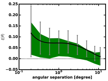
As noted in §2, there is evidence that RGBs and RCs obey different asteroseismic scaling relations, which could lead to systematic differences in their parallaxes, and perhaps a difference in a spatially-correlated offsets from TGAS parallaxes. We present Figures 10 & 11 in order to investigate whether the observed spatial correlations in parallax offset vary with stellar type. We find the two samples to yield consistent signals at all scales, with the RGB sample exhibiting a mildly larger amplitude. Moreover, when averaged over the entire Kepler field, there do not seem to be significant differences in the TGAS and asteroseismic parallax scales as a function of evolutionary type (see §5.5 and Huber et al., in press). We note, furthermore, that this observation also suggests that intrinsic spatial correlations of extinction are not contributing significantly to the signal, because in that case we would expect RC parallaxes to be more spatially-correlated than those of RGBs, since they have larger distances on average than RGBs. However, the RC sample shows mildly smaller, not larger, correlation coefficients than the RGB sample. We discuss asteroseismic parallax scale systematics further in §5.4.

5.3 Bias in observables

As we note in §5.2, spatial correlations should not arise from global biases in the asteroseismic parallaxes. For completeness, however, we perform several checks on the the reliability of the quantities that are used to compute asteroseismic parallaxes.

Figure 12: $V$ magnitudes as derived in this work versus those from APASS (Henden & Munari, 2014), which are consistent within statistical errors (median error bar is shown in the top panel). Grey dashed lines show one-to-one relations. The bottom axes show running medians of the fractional parallax differences (grey curves), with grey error bars representing the standard deviation of the difference within each bin and red error bars representing the statistical error on the median within each bin.

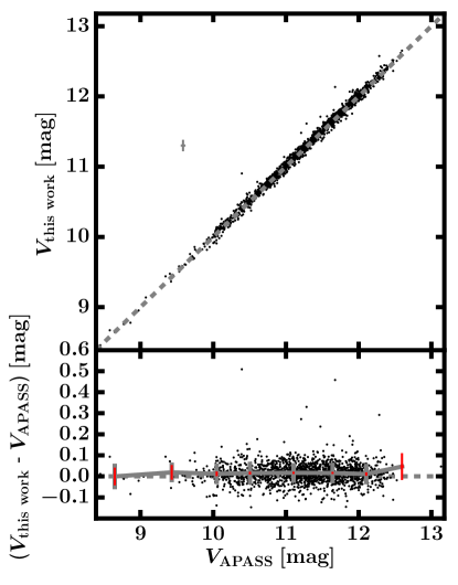
First, we confirmed that our re-reddened $V$ agree with those from APASS (Henden & Munari, 2014) to within statistical errors, as shown in Figure 12.

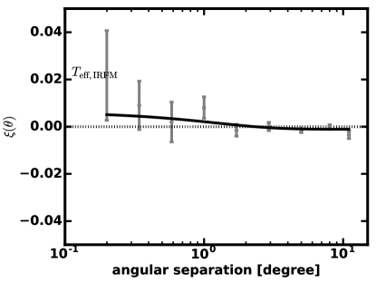
We also tested the effect of using the APOGEE spectroscopic temperature versus an IRFM temperature in computing asteroseismic parallax. The temperature scale does not remove the observed spatial correlation (see §5.4). Nevertheless, there is a different zeropoint offset when using the IRFM temperature scale, which originates from the IRFM being systematically hotter than the APOGEE spectroscopic temperature (see Figure 2).

(a)

(b)

(c)

(d)

(e)

(f)

Figure 13: Same as Figure 8, but for the observables on which asteroseismic parallax depends. Note the difference in scale for the $A_{V}$ panel.

(a)

(b)

(c)

(d)

Figure 14: Continued from Figure 13.

Figure 15: Same as Figures 13 & 14, but for de-extincted $K_{\mathrm{s}}$, $K_{\mathrm{s,\ 0}}$, calculated iteratively, as described in §3.1, and with asteroseismic parallax computed with a $K_{\mathrm{s,\ 0}}$ bolometric correction instead of $F_{\mathrm{bol}}$ from the IRFM, and using $T_{\mathrm{eff,APOGEE}}$ instead of $T_{\mathrm{eff,IRFM}}$. Refer to §5.4 for details.

5.4 Spatial correlation of observables

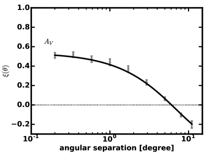
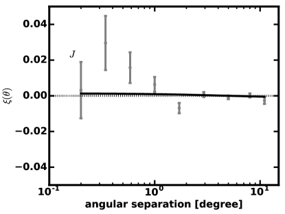
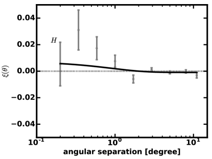
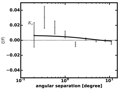
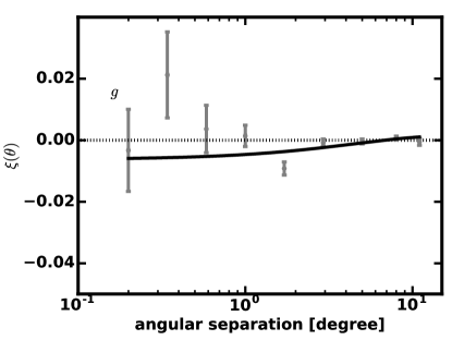
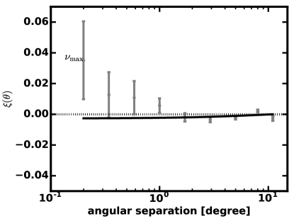
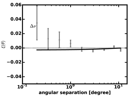
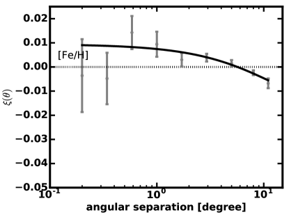
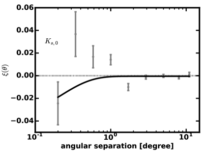
It is possible that the observed spatial dependence of the quantity $\varpi_{\mathrm{TGAS}}-\varpi_{\mathrm{astero}}$ could be the result of spatial correlations in the observables that enter in to the calculation of $\varpi_{\mathrm{astero}}$. We plot all the observable quantities that are used to compute $\varpi_{\mathrm{astero}}$, which are shown in Figures 13 & 14. We have computed a binned Pearson correlation coefficient for these quantities via a modified version of Equation 5:

$$\xi(\theta)\equiv\frac{\sum_{i\neq j}(X_{i}-\langle X\rangle)_{\theta}(X_{j}-\langle X\rangle)_{\theta}}{\sqrt{((X_{i}-\langle X\rangle)^{2})_{\theta}((X_{j}-\langle X\rangle)^{2})_{\theta}}},$$ (9)

where $\langle X\rangle$ is the average value of an observable quantity, $X$, for the entire TGAS-APOKASC sample. The above quantifies, as a function of angular separation, how correlated an observable quantity, $X$, is. Table 2 shows that all observable quantities except $A_{V}$ have negligible spatially-correlated systematic errors, $\sigma_{\mathrm{sys}}$, based on fits to the binned Pearson correlation coefficient, which are mapped to systematic error according to Equation 8.

Unsurprisingly, there are non-negligible spatial correlations in our derived extinctions. In addition to intrinsic spatial clustering of dust in projection, the dust map in Figure 1 shows a region of enhanced extinction in the Kepler field, which is spatially concentrated. Crucially, we do not find significantly different results when we perform our analysis only on the region in which the extinction is the highest ($\ell\lesssim 73^{\circ}$).

Even a systematic spatial correlation at small angular scales (less than $0.1$ degrees) at the level of $0.07$mag in $A_{V}$ would at most translate as a $0.035$mas offset in parallax scales. However, we infer a systematic offset between TGAS and asteroseismic parallaxes of $0.127^{+0.010}_{-0.011}$mas near $0.1$deg for the best-fitting model for the entire TGAS-APOKASC sample. In other words, the correlations in dust cannot account for the correlation we see in TGAS parallaxes.

We performed additional tests to confirm that our result is not due to spatial correlations of extinction propagating into our asteroseismic parallaxes. Figure 15 shows the binned Pearson correlation coefficient for de-extincted $K_{\mathrm{s}}$, $K_{\mathrm{s,\ 0}}$. We note that there is statistically no spatial correlation in $K_{\mathrm{s,\ 0}}$, as there is in $A_{V}$, which is due to the negligible dust extinction in $K_{\mathrm{s}}$ ($A_{K_{\mathrm{s}}}\approx 0.1A_{V}$). We therefore tested a single-band bolometric correction with $K_{\mathrm{s}}$—instead of using $BVJHK_{\mathrm{s}}$, per our fiducial IRFM method described in §3—and found that it does not remove the spatially-correlated parallax offset. We also confirm that using the reddenings derived from stellar models adopted in Huber et al. (in press) instead of those from a dust map does not change our results.

5.5 TGAS-asteroseismic parallax zeropoint

Stassun & Torres (2016a) find that, when compared to 99 eclipsing binaries from Stassun & Torres (2016b) (which have parallaxes with uncertainties of $\sim 200\mu$as), Gaia DR1 parallaxes are smaller by $\sim 200\mu$as. Casertano et al. (2017), however, found no systematic offset above $1\mu$as when comparing with 202 Galactic Cepheids with photometric parallaxes. We find the absolute zeropoint correction suggested by Stassun & Torres (2016a) to over-correct the TGAS parallaxes by about $0.20\pm 0.05$mas (see Figure 7). Though this discrepancy in zeropoints between TGAS and our parallax sample and that of Stassun & Torres (2016a) is likely because the zeropoint offset should be fractional and not absolute, we take the chance here to discuss potential zeropoint systematics in asteroseismic parallax.

One possible bias in asteroseismic parallaxes are systematics in the scaling relations of Equations 1–3. The most evident assumption in using asteroseismic scaling relations to determine stellar radii is the assumption of homology in stellar structure relative to the Sun. Indeed, a growing body of literature indicates that the $\Delta\nu$ scaling relation can deviate by a couple per cent when applied to derive RGB mean densities, compared to asteroseismic stellar models (e.g., White et al., 2011; Miglio et al., 2012; Guggenberger et al., 2016; Sharma et al., 2016). Among dwarfs, comparing asteroseismic radii to radii from Hipparcos parallax and bolometric flux (Silva Aguirre et al., 2012) and to radii from interferometry (Huber et al., 2012) show agreement to within $5\%$. RGB radii comparisons show mixed results (see Huber et al., 2012; Frandsen et al., 2013; Gaulme et al., 2014; Brogaard et al., 2016; Gaulme et al., 2016).

We investigate the validity of scaling relations in Huber et al. (in press) by comparing to Gaia parallaxes by averaging over the entire Kepler field of view. The effect of spatially-correlated offsets in asteroseismic and TGAS parallaxes at the level indicated in this work does not affect the result that asteroseismic radii are consistent with Gaia radii at the $5$ per cent level. We also find evidence for $\Delta\nu$ corrections proposed by Sharma et al. (2016) improving global agreement between the two radii scales.

In light of evidence for red giant $\Delta\nu$ scaling relation corrections, we conservatively apply the $T_{\mathrm{eff}}$- and $\mathrm{[Fe/H]}$-dependent corrections that Sharma et al. (2016) propose to our APOKASC $\Delta\nu$ values. Such corrections do not significantly affect $\log~{}g$ calculations (Hekker et al., 2013), and the significance of our result is not affected by the choice of whether or not to apply $\Delta\nu$ corrections.

Even if the asteroseismic scale is biased with respect to the TGAS parallax scale (which would manifest as a zeropoint offset), the spatial correlation that we retrieve is still valid. Any required corrections to the asteroseismic scaling relations (Equations 1–3) will only be spatially-dependent insofar as the observable quantities that enter in to them (i.e., $g$, $r$, $J$, $H$, $K_{\mathrm{s}}$, $\nu_{\mathrm{max}}$, $\Delta\nu$, $\mathrm{[Fe/H]}$, $T_{\mathrm{eff}}$) are significantly spatially correlated. We demonstrate in §5.4 that no significant spatial correlations exist in these quantities, except in $A_{V}$. Importantly, we have confirmed that the result is insensitive to extinction corrections, which are, in fact, spatially-correlated on the angular scales investigated in this paper.

5.6 Gaia systematics

If the observed difference in TGAS and asteroseismic parallax scales is not due to spatial correlations of asteroseismic parallaxes themselves, then we interpret them as spatially-correlated errors in TGAS parallaxes. There are a few reasons to come to this conclusion. As discussed in Lindegren et al. (2016), for instance, the attitude model of the astrometric solution does not have a high enough temporal resolution to remove small time scale attitude changes. As a result, the Gaia team expects that spatial correlations on scales of a few degrees and less are a result of unmodeled, correlated attitude changes on time scales of minutes, which translate into spatial correlations of degrees and less.

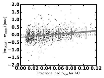
Though we do not have access to the astrometric solution model to independently demonstrate that observed TGAS-asteroseismic parallax offsets are a result of systematic errors in the astrometric solution, we can make inferences based on the published DR1 data. In particular, we show in Figure 16 that the difference in TGAS and asteroseismic parallax scales correlates significantly with the fraction of ‘bad’ across-scan direction observations to total across-scan direction observations. Taking this metric as a proxy for the uncertainty in the across-scan measurement, the correlation corroborates a note in Lindegren et al. (2016) indicating that the across-scan direction measurement error changes parallax solutions in a systematic way, for unknown reasons.

Figure 16: Difference in TGAS and asteroseismic parallax for each star in the TGAS-APOKASC sample, as a function of the ratio of the number of across-scan measurements flagged as ‘bad’ to the total number of across-scan measurements for each star. The straight line is the best-fitting trend, with 1-sigma slopes shown as dashed lines. The standard deviation of parallax difference in bins of the number of ‘bad’ across-scan measurements are shown as error bars.

6 Conclusion

We have independently validated and have quantified spatially-correlated errors in TGAS parallaxes, as predicted by the Gaia team. Our result complements warnings in the Gaia DR1 documentation that there exist systematic uncertainties of amplitude comparable to the statistical uncertainties. For convenience and comparison to future work, we have provided a characteristic scale and amplitude for the spatial correlations: an error of $0.059^{+0.004}_{-0.004}$mas on scales of $0.3$deg, which decreases for larger scales to become $0.011^{+0.006}_{-0.004}$mas at $8$deg. A covariance matrix for the correlated errors in parallax may be computed via Equation 8, using either of the models fit to the observed spatial correlation signal, $\xi(\theta)$, which are provided in Table 1. For any pair of stars, $i$ and $j$, separated by angular distance, $\theta$, their respective entry in a covariance matrix, $\sigma^{2}_{ij}$, would read $\sigma_{ij}^{2}=\xi(\theta)\sigma^{2}$, where $\sigma$ is the statistical error on TGAS parallaxes.

We have done several checks on our result, which is robust to:

1. the dust prescription that is used — without significant differences in the observed spatial correlation in parallax error when omitting the region of the Kepler field of view most affected by dust or when using a stellar model extinction instead of a dust map extinction;

2. the evolutionary status of the stars used to calculate asteroseismic parallax, with both first ascent red giant branch and red clump parallaxes indicating the same spatially-correlated parallax offset with respect to TGAS parallaxes;

3. whether or not a $BVJHK_{\mathrm{s}}$ bolometric correction is used to compute asteroseismic parallax or a $K_{\mathrm{s}}$-band bolometric correction is used;

4. the temperature scale used – whether it be the spectroscopic $T_{\mathrm{eff,APOGEE}}$ scale or the IRFM scale, $T_{\mathrm{eff,IRFM}}$;

5. and whether or not $\Delta\nu$ corrections are applied to the asteroseismic scaling relations.

At this point, we cannot test the possibility of correlations on scales larger than $10$deg due to the $\sim 10^{\circ}\times 10^{\circ}$ spatial extent of the Kepler field of view. Future work could quantify spatial correlations on larger scales using, e.g., K2 asteroseismology, which would yield parallaxes for objects separated by the largest angular scales. We encourage the use of the spatial covariance functional form when computing quantities that depend on TGAS parallaxes, especially in light of the delay of Gaia DR2 to April 2018.

Appendix A Alternate formulations of spatial correlation

Here, we present representations of spatially-correlated parallax offsets that are complementary to the Pearson correlation coefficient presented in the text. We prefer the Pearson correlation coefficient formulation because it is directly mappable to a covariance function, but we include the following representations for completeness.

A.1 Angular correlation function

Figure 17: The angular correlation function of the quantity $(\varpi_{\mathrm{TGAS}}-\varpi_{\mathrm{astero}})/\sqrt{(\sigma_{\varpi_{\mathrm{TGAS}}}^{2}+\sigma_{\varpi_{\mathrm{astero}}}^{2})}$, which will be positive for offsets that are positively correlated (i.e., differences between TGAS and asteroseismic parallaxes are in the same sense for pairs of stars at a given angular scale), zero in the absence of spatially-correlated parallax offsets, and negative for anti-correlated TGAS parallax offsets (i.e., differences between TGAS and asteroseismic parallaxes are in opposite senses for pairs of stars at a given angular scale). Grey points are the observed angular correlation function values, with error bars assuming Poisson statistics; the black dashed line indicates a null correlation. See the Appendix for details.

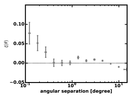
The angular correlation function, often used in cosmological contexts, may be calculated using the Landy-Szalay estimator (Landy & Szalay, 1993):

$$\xi(\theta)=\frac{\langle\mathrm{DD}\rangle_{\theta}-2\langle\mathrm{DR}\rangle_{\theta}+\langle\mathrm{RR}\rangle_{\theta}}{\langle\mathrm{RR}\rangle_{\theta}},$$

where $D$ in our case refers to an observed value of the quantity $(\varpi_{\mathrm{TGAS}}-\varpi_{\mathrm{astero}})/\sqrt{(\sigma_{\varpi_{\mathrm{TGAS}}}^{2}+\sigma_{\varpi_{\mathrm{astero}}}^{2})}$ for a star, and $R$ refers to a sample drawn from the observed values of the normalized parallax difference, but with positions drawn randomly from within the Kepler field of view, making use of K2fov (Mullally et al., 2016); $\langle\rangle_{\theta}$ represents the expected value of that quantity for pairs of points separated by angular distance $\theta$. We compute this statistic with TreeCorr (Jarvis et al., 2004). Error bars for each angular bin are assigned based on Poisson statistics. This statistic is widely-used in cosmology to compute correlation functions. Although complementary to, the angular correlation coefficient will in general not be equivalent to the Pearson correlation coefficient. However, it does explicitly account for stochasticity in the spatial distribution of the TGAS-APOKASC sample. Results using this approach are qualitatively similar, as seen in comparing Figures 8 & 17.

A.2 Binned absolute difference

Figure 18: A binned absolute difference in parallax scales shows excess difference in the scales for angular scales less than a few degrees, offering an alternate representation of the main result of spatially-correlated offsets in asteroseismic and TGAS parallax scales (see Figure 8). See the Appendix for details.

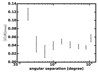
Most intuitive is the simple measure

$$\langle\delta\rangle(\theta)=\sqrt{\langle|(\varpi_{\mathrm{TGAS,i}}-\varpi_{\mathrm{astero,i}})(\varpi_{\mathrm{TGAS,j}}-\varpi_{\mathrm{astero,j}})|\rangle}_{\theta},$$

which is a measure of the absolute difference in the parallax scales computed by binning pairs of stars, $i$ and $j$, separated by an angular distance, $\theta$. This scale will not necessarily be the same as the scale we present in the text, and in particular is insensitive to the sign of the (anti-)correlation. Figure 18 shows this measure for the TGAS-APOKASC sample.

References

- Akaike (1973) Akaike, H. 1973, in 2nd International Symposium on Information Theory, Petrov, B.N.; Csáki, F., 267–281
- Astraatmadja & Bailer-Jones (2016) Astraatmadja, T. L., & Bailer-Jones, C. A. L. 2016, ApJ, 833, 119
- Bailer-Jones (2015) Bailer-Jones, C. A. L. 2015, PASP, 127, 994
- Borucki et al. (2010) Borucki, W. J., Koch, D., Basri, G., et al. 2010, Science, 327, 977
- Bovy et al. (2016) Bovy, J., Rix, H.-W., Green, G. M., Schlafly, E. F., & Finkbeiner, D. P. 2016, ApJ, 818, 130
- Brogaard et al. (2016) Brogaard, K., Jessen-Hansen, J., Handberg, R., et al. 2016, Astronomische Nachrichten, 337, 793
- Brown et al. (1991) Brown, T. M., Gilliland, R. L., Noyes, R. W., & Ramsey, L. W. 1991, ApJ, 368, 599
- Brown et al. (2011) Brown, T. M., Latham, D. W., Everett, M. E., & Esquerdo, G. A. 2011, AJ, 142, 112
- Casertano et al. (2017) Casertano, S., Riess, A. G., Bucciarelli, B., & Lattanzi, M. G. 2017, AAP, 599, A67
- Chaplin et al. (2008) Chaplin, W. J., Houdek, G., Appourchaux, T., et al. 2008, AAP, 485, 813
- Christensen-Dalsgaard (1993) Christensen-Dalsgaard, J. 1993, in Astronomical Society of the Pacific Conference Series, Vol. 42, GONG 1992. Seismic Investigation of the Sun and Stars, ed. T. M. Brown, 347
- Davies et al. (2017) Davies, G. R., Lund, M. N., Miglio, A., et al. 2017, AAP, 598, L4
- Davison & Hinkley (1997) Davison, A. C., & Hinkley, D. V. 1997, Bootstrap Methods and their Applications (Cambridge: Cambridge University Press)
- De Ridder et al. (2016) De Ridder, J., Molenberghs, G., Eyer, L., & Aerts, C. 2016, AAP, 595, L3
- Drimmel et al. (2003) Drimmel, R., Cabrera-Lavers, A., & López-Corredoira, M. 2003, AAP, 409, 205
- Foreman-Mackey et al. (2013) Foreman-Mackey, D., Hogg, D. W., Lang, D., & Goodman, J. 2013, PASP, 125, 306
- Frandsen et al. (2013) Frandsen, S., Lehmann, H., Hekker, S., et al. 2013, AAP, 556, A138
- Gaia Collaboration et al. (2016a) Gaia Collaboration, Prusti, T., de Bruijne, J. H. J., et al. 2016a, AAP, 595, A1
- Gaia Collaboration et al. (2016b) Gaia Collaboration, Brown, A. G. A., Vallenari, A., et al. 2016b, AAP, 595, A2
- Gaulme et al. (2014) Gaulme, P., Jackiewicz, J., Appourchaux, T., & Mosser, B. 2014, ApJ, 785, 5
- Gaulme et al. (2016) Gaulme, P., McKeever, J., Jackiewicz, J., et al. 2016, ApJ, 832, 121
- González Hernández & Bonifacio (2009) González Hernández, J. I., & Bonifacio, P. 2009, AAP, 497, 497
- Gould et al. (2016) Gould, A., Kollmeier, J. A., & Sesar, B. 2016, ArXiv e-prints, arXiv:1609.06315
- Green et al. (2015) Green, G. M., Schlafly, E. F., Finkbeiner, D. P., et al. 2015, ApJ, 810, 25
- Guggenberger et al. (2016) Guggenberger, E., Hekker, S., Basu, S., & Bellinger, E. 2016, MNRAS, 460, 4277
- Hekker et al. (2013) Hekker, S., Elsworth, Y., Basu, S., et al. 2013, MNRAS, 434, 1668
- Henden & Munari (2014) Henden, A., & Munari, U. 2014, Contributions of the Astronomical Observatory Skalnate Pleso, 43, 518
- Høg et al. (2000) Høg, E., Fabricius, C., Makarov, V. V., et al. 2000, AAP, 355, L27
- Huber et al. (2009) Huber, D., Stello, D., Bedding, T. R., et al. 2009, Communications in Asteroseismology, 160, 74
- Huber et al. (2012) Huber, D., Ireland, M. J., Bedding, T. R., et al. 2012, ApJ, 760, 32
- Jao et al. (2016) Jao, W.-C., Henry, T. J., Riedel, A. R., et al. 2016, ApJL, 832, L18
- Jarvis et al. (2004) Jarvis, M., Bernstein, G., & Jain, B. 2004, MNRAS, 352, 338
- Kjeldsen & Bedding (1995) Kjeldsen, H., & Bedding, T. R. 1995, AAP, 293, 87
- Landy & Szalay (1993) Landy, S. D., & Szalay, A. S. 1993, ApJ, 412, 64
- Lindegren et al. (2016) Lindegren, L., Lammers, U., Bastian, U., et al. 2016, AAP, 595, A4
- Loh (2008) Loh, J. M. 2008, ApJ, 681, 726
- Majewski et al. (2015) Majewski, S. R., Schiavon, R. P., Frinchaboy, P. M., et al. 2015, ArXiv e-prints, arXiv:1509.05420
- Mamajek et al. (2015) Mamajek, E. E., Prsa, A., Torres, G., et al. 2015, ArXiv e-prints, arXiv:1510.07674
- Marshall et al. (2006) Marshall, D. J., Robin, A. C., Reylé, C., Schultheis, M., & Picaud, S. 2006, AAP, 453, 635
- Michalik et al. (2015) Michalik, D., Lindegren, L., & Hobbs, D. 2015, AAP, 574, A115
- Miglio et al. (2012) Miglio, A., Brogaard, K., Stello, D., et al. 2012, MNRAS, 419, 2077
- Mosser et al. (2014) Mosser, B., Benomar, O., Belkacem, K., et al. 2014, AAP, 572, L5
- Mullally et al. (2016) Mullally, F., Barclay, T., & Barentsen, G. 2016, ascl:1601.009. http://dx.doi.org/10.5281/zenodo.44283
- Pinsonneault et al. (2012) Pinsonneault, M. H., An, D., Molenda-Żakowicz, J., et al. 2012, ApJS, 199, 30
- Pinsonneault et al. (2014) Pinsonneault, M. H., Elsworth, Y., Epstein, C., et al. 2014, ApJS, 215, 19
- Rodrigues et al. (2014) Rodrigues, T. S., Girardi, L., Miglio, A., et al. 2014, MNRAS, 445, 2758
- SDSS Collaboration et al. (2016) SDSS Collaboration, Albareti, F. D., Allende Prieto, C., et al. 2016, ArXiv e-prints, arXiv:1608.02013
- Sesar et al. (2017) Sesar, B., Fouesneau, M., Price-Whelan, A. M., et al. 2017, ApJ, 838, 107
- Sharma et al. (2016) Sharma, S., Stello, D., Bland-Hawthorn, J., Huber , D., & Bedding, T. R. 2016, ApJ, 822, 15
- Silva Aguirre et al. (2012) Silva Aguirre, V., Casagrande, L., Basu, S., et al. 2012, ApJ, 757, 99
- Skrutskie et al. (2006) Skrutskie, M. F., Cutri, R. M., Stiening, R., et al. 2006, AJ, 131, 1163
- Stassun & Torres (2016a) Stassun, K. G., & Torres, G. 2016a, The Astrophysical Journal Letters, 831, L6. http://stacks.iop.org/2041-8205/831/i=1/a=L6
- Stassun & Torres (2016b) —. 2016b, AJ, 152, 180
- Stello et al. (2013) Stello, D., Huber, D., Bedding, T. R., et al. 2013, ApJL, 765, L41
- Tassoul (1980) Tassoul, M. 1980, ApJS, 43, 469
- White et al. (2011) White, T. R., Bedding, T. R., Stello, D., et al. 2011, The Astrophysical Journal, 743, 161. http://stacks.iop.org/0004-637X/743/i=2/a=161
- Zasowski et al. (2015) Zasowski, G., An, D., & Pinsonneault, M. 2015, in Astrophysics and Space Science Proceedings, Vol. 39, Asteroseismology of Stellar Populations in the Milky Way, ed. A. Miglio, P. Eggenberger, L. Girardi, & J. Montalbán, 83
- Zasowski et al. (2013) Zasowski, G., Johnson, J. A., Frinchaboy, P. M., et al. 2013, AJ, 146, 81