Logarithmic and Riesz Equilibrium for Multiple Sources on the Sphere — the Exceptional Case

Abstract

We consider the minimal discrete and continuous energy problems on the unit sphere $\mathbb{S}^{d}$ in the Euclidean space $\mathbb{R}^{d+1}$ in the presence of an external field due to finitely many localized charge distributions on $\mathbb{S}^{d}$, where the energy arises from the Riesz potential $1/r^{s}$ ($r$ is the Euclidean distance) for the critical Riesz parameter $s=d-2$ if $d\geq 3$ and the logarithmic potential $\log(1/r)$ if $d=2$. Individually, a localized charge distribution is either a point charge or assumed to be rotationally symmetric. The extremal measure solving the continuous external field problem for weak fields is shown to be the uniform measure on the sphere but restricted to the exterior of spherical caps surrounding the localized charge distributions. The radii are determined by the relative strengths of the generating charges. Furthermore, we show that the minimal energy points solving the related discrete external field problem are confined to this support. For $d-2\leq s<d$, we show that for point sources on the sphere, the equilibrium measure has support in the complement of the union of specified spherical caps about the sources. Numerical examples are provided to illustrate our results.

To Ian Sloan, an outstanding mathematician, mentor, and colleague,
with much appreciation for his insights, guidance, and friendship.

1 Introduction

Let $\mathbb{S}^{d}{\,:=\,}\{\mathbf{x}\in\mathbb{R}^{d+1}:|\mathbf{x}|=1\}$ be the unit sphere in $\mathbb{R}^{d+1}$, where $|\mathbf{\cdot}|$ denotes the Euclidean norm. Given a compact set $E\subset\mathbb{S}^{d}$, consider the class $\mathcal{M}(E)$ of unit positive Borel measures supported on $E$. For $0<s<d$ the Riesz $s$-potential and Riesz $s$-energy of a measure $\mu\in\mathcal{M}(E)$ are given, respectively, by

$$U_{s}^{\mu}(\mathbf{x}){\,:=\,}\int k_{s}(\mathbf{x},\mathbf{y})\operatorname{\mathrm{d}}\mu(\mathbf{y}),\ \ \mathbf{x}\in\mathbb{R}^{d+1},\quad\mathcal{I}_{s}(\mu){\,:=\,}\int\int k_{s}(\mathbf{x},\mathbf{y})\operatorname{\mathrm{d}}\mu(\mathbf{x})\operatorname{\mathrm{d}}\mu(\mathbf{y}),$$

where $k_{s}(\mathbf{x},\mathbf{y}){\,:=\,}|\mathbf{x}-\mathbf{y}|^{-s}$ for $s>0$ is the so-called Riesz kernel. For the case $s=0$ we use the logarithmic kernel $k_{0}(\mathbf{x},\mathbf{y}){\,:=\,}\log(1/|\mathbf{x}-\mathbf{y}|)$. The $s$-capacity of $E$ is then defined as $C_{s}(E){\,:=\,}1/W_{s}(E)$ for $s>0$ and $C_{0}(E)=\exp(-W_{0}(E))$, where $W_{s}(E){\,:=\,}\inf\{\mathcal{I}_{s}(\mu):\mu\in\mathcal{M}(E)\}$. A property is said to hold quasi-everywhere (q.e.) if the exceptional set has $s$-capacity zero. When $C_{s}(E)>0$, there exists a unique minimizer $\mu_{E}=\mu_{s,E}$, called the $s$-equilibrium measure on $E$, such that $\mathcal{I}_{s}(\mu_{E})=W_{s}(E)$. The $s$-equilibrium measure is just the normalized surface area measure on $\mathbb{S}^{d}$ which we denote with $\sigma_{d}$. For more details see (Landkof1972, , Chapter II).

We remind the reader that the $s$-energy of $\mathbb{S}^{d}$ is given by

$$U_{s}^{\sigma_{d}}(\mathbf{x})=\mathcal{I}_{s}(\sigma_{d})=W_{s}(\mathbb{S}^{d})=\frac{\operatorname{\Gamma}(d)\operatorname{\Gamma}((d-s)/2)}{2^{s}\operatorname{\Gamma}(d/2)\operatorname{\Gamma}(d-s/2)},\qquad 0<s<d,$$ (1)

and the logarithmic energy of $\mathbb{S}^{d}$ is given by

$$\begin{split}U_{0}^{\sigma_{d}}(\mathbf{x})=\mathcal{I}_{0}(\sigma_{d})=W_{0}(\mathbb{S}^{d})&=\frac{\mathrm{d}W_{s}(\mathbb{S}^{d})}{\mathrm{d}s}\Big{|}_{s=0}=-\log(2)+\frac{1}{2}\left(\operatorname{\psi}(d)-\operatorname{\psi}(d/2)\right),\end{split}$$

where $\operatorname{\psi}(s){\,:=\,}\operatorname{\Gamma}^{\prime}(s)/\operatorname{\Gamma}(s)$ is the digamma function. Using cylindrical coordinates

$$\mathbf{x}=(\sqrt{1-u^{2}}\;\overline{\mathbf{x}},u),\qquad-1\leq u\leq 1,\;\overline{\mathbf{x}}\in\mathbb{S}^{d-1},$$ (2)

we can write the decomposition

$$\operatorname{\mathrm{d}}\sigma_{d}(\mathbf{x})=\frac{\omega_{d-1}}{\omega_{d}}\left(1-u^{2}\right)^{d/2-1}\,\operatorname{\mathrm{d}}u\,\operatorname{\mathrm{d}}\sigma_{d-1}(\overline{\mathbf{x}}).$$ (3)

Here $\omega_{d}$ is the surface area of $\mathbb{S}^{d}$ and the ratio of these areas can be evaluated as

$$\omega_{0}=2,\quad\frac{\omega_{d}}{\omega_{d-1}}=\int_{-1}^{1}\left(1-u^{2}\right)^{d/2-1}\operatorname{\mathrm{d}}u=\frac{\sqrt{\pi}\operatorname{\Gamma}(d/2)}{\operatorname{\Gamma}((d+1)/2)}=2^{d-1}\frac{\left[\operatorname{\Gamma}(d/2)\right]^{2}}{\operatorname{\Gamma}(d)}.$$ (4)

We shall refer to a non-negative lower semi-continuous function $Q:\mathbb{S}^{d}\to[0,\infty]$ such that $Q(\mathbf{x})<\infty$ on a set of positive Lebesgue surface area measure as an external field. The weighted energy associated with $Q$ is then given by

$$I_{Q}(\mu){\,:=\,}\mathcal{I}_{s}(\mu)+2\int Q(\mathbf{x})\operatorname{\mathrm{d}}\mu(\mathbf{x}).$$ (5)

Definition 1

The minimal energy problem on the sphere in the presence of the external field $Q$ refers to the quantity

$$V_{Q}{\,:=\,}\inf\left\{I_{Q}(\mu):\mu\in\mathcal{M}(\mathbb{S}^{d})\right\}.$$ (6)

A measure $\mu_{Q}=\mu_{Q,s}\in\mathcal{M}(\mathbb{S}^{d})$ such that $I_{Q}(\mu_{Q})=V_{Q}$ is called an $s$-extremal (or $s$-equilibrium) measure associated with $Q$.

The discretized version of the minimal $s$-energy problem is also of interest. The associated optimal point configurations have a variety of possible applications, such as for generating radial basis functions on the sphere that are used in the numerical solutions to PDEs (see, e.g., LeGSloWen2012a , LeGSloWen2012b ).

Given a positive integer $N$, we consider the optimization problem

$$\mathcal{E}_{Q,N}{\,:=\,}\min_{\{\mathbf{x}_{1},\ldots,\mathbf{x}_{N}\}\subset\mathbb{S}^{d}}\sum_{1\leq i\not=j\leq N}\big{[}k_{s}(\mathbf{x}_{i},\mathbf{x}_{j})+Q(\mathbf{x}_{i})+Q(\mathbf{x}_{j})\big{]}.$$ (7)

A system that minimizes the discrete energy is called an optimal (minimal) $s$-energy $N$-point configuration w.r.t. $Q$. The field-free case $Q\equiv 0$ is particularly important.

The following Frostman-type result as stated in DraSaf2007 summarizes the existence and uniqueness properties for $s$-equilibrium measures on $\mathbb{S}^{d}$ in the presence of external fields (see also (SafTot1997, , Theorem I.1.3) for the complex plane case and Zorii2003 for more general spaces).

Proposition 1

Let $0\leq s<d$. For the minimal $s$-energy problem on $\mathbb{S}^{d}$ with external field $Q$ the following properties hold:

1. $V_{Q}$ is finite.

2. There exists a unique $s$-equilibrium measure $\mu_{Q}=\mu_{Q,s}\in\mathcal{M}(\mathbb{S}^{d})$ associated with $Q$. Moreover, the support $S_{Q}$ of this measure is contained in the compact set $E_{M}{\,:=\,}\{\mathbf{x}\in\mathbb{S}^{d}:Q(\mathbf{x})\leq M\}$ for some $M>0$.

3. The measure $\mu_{Q}$ satisfies the variational inequalities

   $$U_{s}^{\mu_{Q}}(\mathbf{x})+Q(\mathbf{x}) \geq F_{Q}\quad\text{q.e. on $\mathbb{S}^{d}$,}$$ (8)

   $$U_{s}^{\mu_{Q}}(\mathbf{x})+Q(\mathbf{x}) \leq F_{Q}\quad\text{for all $\mathbf{x}\in S_{Q}$,}$$ (9)

   where

   $$F_{Q}{\,:=\,}V_{Q}-\int Q(\mathbf{x})\operatorname{\mathrm{d}}\mu_{Q}(\mathbf{x}).$$ (10)

4. Inequalities (8) and (9) completely characterize the extremal measure $\mu_{Q}$ in the sense that if $\nu\in\mathcal{M}(\mathbb{S}^{d})$ is a measure with finite $s$-energy such that

   $$U_{s}^{\nu}(\mathbf{x})+Q(\mathbf{x}) \geq C\quad\text{q.e. on $\mathbb{S}^{d}$,}$$ (11)

   $$U_{s}^{\nu}(\mathbf{x})+Q(\mathbf{x}) \leq C\quad\text{for all $\mathbf{x}\in\operatorname{supp}(\nu)$}$$ (12)

   for some constant $C$, we have then $\mu_{Q}=\nu$ and $F_{Q}=C$.

Remark 1

We note that a similar statement holds true when $\mathbb{S}^{d}$ is replaced by any compact subset $K\subset\mathbb{S}^{d}$ of positive $s$-capacity.

The explicit determination of $s$-equilibrium measures or their support is not an easy task. In DraSaf2007 an external field exerted by a single point mass on the sphere was applied to establish that, in the field-free case, minimal $s$-energy $N$-point systems on $\mathbb{S}^{d}$, as defined in (7), are “well-separated” for $d-2<s<d$. Axis-supported external fields were studied in BraDraSaf2009 and rotationally invariant external fields on $\mathbb{S}^{2}$ in Bil2016 . The separation of minimal $s$-energy $N$-point configurations for more general external fields, namely Riesz $s$-potentials of signed measures with negative charge outside the unit sphere, was established in BraDraSaf2014 .

Here we shall focus primarily on the exceptional case when $s=d-2$ and $Q$ is the external field exerted by finitely many localized charge distributions. Let $\mathbf{a}_{1},\mathbf{a}_{2},\dots,\mathbf{a}_{m}\in\mathbb{S}^{d}$ be $m$ fixed points with associated positive charges $q_{1},q_{2},\dots,q_{m}$. Then the external field is given by

$$Q(\mathbf{x}):=\sum_{i=1}^{m}q_{i}\,k_{d-2}(\mathbf{a}_{i},\mathbf{x}).$$ (13)

For sufficiently small charges $q_{1},\dots,q_{m}$ we completely characterize the ${(d-2)}$-equilibrium measure for the external field (13).

The outline of the paper is as follows. In Section 2, we introduce some notion from potential theory utilized in our analysis. In Section 3, we present the important case of the unit sphere in the $3$-dimensional space and logarithmic interactions. An interesting corollary in its own right for discrete external fields in the complex plane is exhibited as well. The situation when $d\geq 3$, considered in Section 4, is more involved as there is a loss of mass in the balayage process. Finally, in Section 5, we derive a result on regions free of optimal points and formulate an open problem.

2 Signed Equilibria, Mhaskar-Saff $\mathcal{F}$-Functional, and Balayage

A significant role in our analysis is played by the so-called signed equilibrium (see BraDraSaf2009 ; BraDraSaf2014 ).

Definition 2

Given a compact subset $E\subset\mathbb{R}^{p}$, $p\geq 3$, and an external field $Q$, we call a signed measure $\eta_{E,Q}=\eta_{E,Q,s}$ supported on $E$ and of total charge $\eta_{E,Q}(E)=1$ a signed $s$-equilibrium on $E$ associated with $Q$ if its weighted Riesz $s$-potential is constant on $E$:

$$U_{s}^{\eta_{E,Q}}(\mathbf{x})+Q(\mathbf{x})=F_{E,Q}\qquad\text{for all $\mathbf{x}\in E$.}$$ (14)

We note that if the signed equilibrium exists, it is unique (see (BraDraSaf2009, , Lemma 23)). In view of (8) and (9), the signed equilibrium on $S_{Q}$ is actually a non-negative measure and coincides with the $s$-extremal measure associated with $Q$, and hence can be obtained by solving a singular integral equation on $S_{Q}$. Moreover, for the equilibrium support we have that $S_{Q}\subset{\rm supp}(\eta_{E,Q}^{+})$ whenever $S_{Q}\subset E\subset\mathbb{S}^{d}$ (see (BraDraSaf2014, , Theorem 9)).

An important tool in our analysis is the Riesz analog of the Mhaskar-Saff $F$-functional from classical logarithmic potential theory in the plane (see MhaSaf1985 and (SafTot1997, , Chapter IV, p. 194)).

Definition 3

The $\mathcal{F}_{s}$-functional of a compact subset $K\subset\mathbb{S}^{d}$ of positive $s$-capacity is defined as

$$\mathcal{F}_{s}(K){\,:=\,}W_{s}(K)+\int Q(\mathbf{x})\,\operatorname{\mathrm{d}}\mu_{K}(\mathbf{x}),$$ (15)

where $W_{s}(K)$ is the $s$-energy of $K$ and $\mu_{K}$ is the $s$-equilibrium measure on $K$.

Remark 2

As pointed out in BraDraSaf2009 ; BraDraSaf2014 , when $d-2\leq s<d$, a relationship exists between the signed $s$-equilibrium constant in (14) and the $\mathcal{F}_{s}$-functional (15), namely $\mathcal{F}_{s}(K)=F_{K,Q}$. Moreover, the equilibrium support minimizes the $\mathcal{F}$-functional; i.e., if $d-2\leq s<d$ and $Q$ is an external field on $\mathbb{S}^{d}$, then the $\mathcal{F}_{s}$-functional is minimized for $S_{Q}=\operatorname{supp}(\mu_{Q})$ (see (BraDraSaf2009, , Theorem 9)).

A tool we use extensively is the Riesz $s$-balayage measure (see (Landkof1972, , Section 4.5)). Given a measure $\nu$ supported on $\mathbb{S}^{d}$ and a compact subset $K\subset\mathbb{S}^{d}$, the measure $\widehat{\nu}:=\operatorname{Bal}_{s}(\nu,K)$ is called the Riesz $s$-balayage of $\nu$ onto $K$, $d-2\leq s<d$, if $\widehat{\nu}$ is supported on $K$ and

$$\begin{split}U_{s}^{\widehat{\nu}}(\mathbf{x})&=U_{s}^{\nu}(\mathbf{x})\qquad\text{on $K$,}\\ U_{s}^{\widehat{\nu}}(\mathbf{x})&\leq U_{s}^{\nu}(\mathbf{x})\qquad\text{on $\mathbb{S}^{d}$.}\end{split}$$ (16)

In general, there is some loss of mass, namely $\widehat{\nu}(\mathbb{S}^{d})<\nu(\mathbb{S}^{d})$. However, in the logarithmic interaction case $s=0$ and $d=2$, the mass of the balayage measures is preserved, but as in the classical complex plane potential theory we have equality of potentials up to a constant term

$$\begin{split}U_{0}^{\widehat{\nu}}(\mathbf{x})&=U_{0}^{\nu}(\mathbf{x})+C\qquad\text{on $K$,}\\ U_{0}^{\widehat{\nu}}(\mathbf{x})&\leq U_{0}^{\nu}(\mathbf{x})+C\qquad\text{on $\mathbb{S}^{2}$.}\end{split}$$ (17)

Balayage of a signed measure $\eta$ is achieved by taking separately the balayage of its positive and its negative part in the Jordan decomposition $\eta=\eta^{+}-\eta^{-}$. An important property is that we can take balayage in steps: if $F\subset K\subset\mathbb{S}^{d}$, then

$$\operatorname{Bal}_{s}(\nu,F)=\operatorname{Bal}_{s}(\operatorname{Bal}_{s}(\nu,K),F).$$ (18)

We also use the well-known relation

$$\operatorname{Bal}_{s}(\nu,K)=\nu_{|_{K}}+\operatorname{Bal}_{s}(\nu_{|_{\mathbb{S}^{d}\setminus K}},K).$$ (19)

3 Logarithmic Interactions on $\mathbb{S}^{2}$

We first state and prove our main theorem for the case of logarithmic interactions on $\mathbb{S}^{2}$. We associate with $Q$ (or equivalently with $\{\mathbf{a}_{i}\}$ and $\{q_{i}\}$) the total charge

$$q:=q_{1}+\cdots+q_{m}$$

the vector

$$\bm{\epsilon}=(\epsilon_{1},\dots,\epsilon_{m}),\qquad\epsilon_{i}:=2\,\sqrt{\frac{q_{i}}{1+q}},\quad i=1,\dots,m,$$ (20)

and the set

$$\Sigma_{\bm{\epsilon}}=\bigcap_{i=1}^{m}\Sigma_{i,\epsilon_{i}},\qquad\Sigma_{i,\epsilon}:=\big{\{}\mathbf{x}\in\mathbb{S}^{2}:|\mathbf{x}-\mathbf{a}_{i}|\geq\epsilon\big{\}},\quad i=1,\dots,m,\,\epsilon\geq 0.$$ (21)

More generally, with any vector $\bm{\gamma}=(\gamma_{1},\dots,\gamma_{m})$ with non-negative components we associate the set $\Sigma_{\bm{\gamma}}=\bigcap_{i=1}^{m}\Sigma_{i,\gamma_{i}}$. Note: if $\bm{\gamma}\leq\bm{\epsilon}$ (i.e., $\gamma_{i}\leq\epsilon_{i}$, $1\leq i\leq m$), then $\Sigma_{\bm{\epsilon}}\subset\Sigma_{\bm{\gamma}}$.

Theorem 3.1

Let $d=2$ and $s=0$. Let $Q$, $\bm{\epsilon}$, and $\Sigma_{\bm{\epsilon}}$ be defined by (13), (20), and (21). Suppose that $\Sigma_{i,\epsilon_{i}}^{c}\cap\Sigma_{j,\epsilon_{j}}^{c}=\emptyset$, $1\leq i<j\leq m$ ($K^{c}$ denotes the complement of $K$ relative to the sphere). Then the logarithmic extremal measure associated with $Q$ is $\mu_{Q}=\left(1+q\right){\sigma_{2}}_{|_{\Sigma_{\bm{\epsilon}}}}$ and the extremal support is $S_{Q}=\Sigma_{\bm{\epsilon}}$.

Remark 3

The theorem has the following electrostatics interpretation. As positively charged particles $\mathbf{a}_{i}$ are introduced on a positively pre-charged unit sphere, they create charge-free regions which we call regions of electrostatic influence. The theorem then states that if the potential interaction is logarithmic and the charges of the particles are sufficiently small (so that the regions of influence do not overlap), then these regions are perfect spherical caps $\Sigma_{i,\epsilon_{i}}^{c}$ whose radii depend only on the amount of charge and the position of the particles. In Section 5, we partially investigate what happens when the $q_{i}$’s increase beyond the critical values imposed by the non-overlapping conditions $\Sigma_{i,\epsilon_{i}}^{c}\cap\Sigma_{i,\epsilon_{j}}^{c}=\emptyset$, $1\leq i<j\leq m$.

Proof

Let $m=1$. This case has already been solved in BraDraSaf2009 . By (BraDraSaf2009, , Theorem 17), the signed equilibrium on $\Sigma_{\gamma}$ associated with $Q(\mathbf{x}):=q\log\frac{1}{|\mathbf{x}-\mathbf{a}|}$, $\mathbf{a}\in\mathbb{S}^{2}$, is given by

$$\eta_{\Sigma_{\gamma},Q} =\left(1+q\right)\operatorname{Bal}_{0}(\sigma_{2},\Sigma_{\gamma})-q\,\operatorname{Bal}_{0}(\delta_{\mathbf{a}},\Sigma_{\gamma})$$

$$=\left(1+q\right){\sigma_{2}}_{|_{\Sigma_{\gamma}}}+\left(1+q\right)\left(\frac{\gamma^{2}}{4}-\frac{q}{1+q}\right)\beta,$$ (22)

where $\beta$ is the normalized Lebesgue measure on the boundary circle of $\Sigma_{\gamma}$.

The logarithmic extremal measure on $\mathbb{S}^{2}$ associated with $Q$ is then given by

$$\mu_{Q}=\left(1+q\right){\sigma_{2}}_{|_{\Sigma_{\epsilon}}},\qquad\text{where $\epsilon=2\,\sqrt{\frac{q}{1+q}}$.}$$

Let $\xi:=\langle\mathbf{x},\mathbf{a}\rangle$ and $\gamma^{2}=2(1-t)$, where $t$ is the projection of the boundary circle $\partial\Sigma_{\gamma}$ onto the $\mathbf{a}$-axis. For future reference, by (BraDraSaf2009, , Lemmas 39 and 41) we have

$$U_{0}^{\operatorname{Bal}_{0}(\sigma_{2},\Sigma_{\gamma})}(\mathbf{x})=\begin{cases}W_{0}(\Sigma_{\gamma}),&\mathbf{x}\in\Sigma_{\gamma},\\[5.0pt] W_{0}(\Sigma_{\gamma})+\dfrac{1}{2}\log\dfrac{1+t}{1+\xi},&\mathbf{x}\in\Sigma_{\gamma}^{c}\end{cases}$$ (23)

and

$$U_{0}^{\operatorname{Bal}_{0}(\delta_{\mathbf{a}},\Sigma_{\gamma})}(\mathbf{x})=U_{0}^{\delta_{\mathbf{a}}}(\mathbf{x})+\begin{cases}\dfrac{1}{2}\log\dfrac{1-t}{1+t}-\dfrac{1}{2}\log\dfrac{1-t}{2},&\mathbf{x}\in\Sigma_{\gamma},\\[5.0pt] \dfrac{1}{2}\log\dfrac{1-\xi}{1+\xi}-\dfrac{1}{2}\log\dfrac{1-t}{2},&\mathbf{x}\in\Sigma_{\gamma}^{c}.\end{cases}$$ (24)

Moreover, $\widehat{\nu}=\operatorname{Bal}_{0}({\sigma_{2}}_{|_{\Sigma_{\gamma}^{c}}},\Sigma_{\gamma})$ and $\widehat{\delta_{\mathbf{a}}}=\operatorname{Bal}_{0}(\delta_{\mathbf{a}},\Sigma_{\gamma})$ are multiples of $\beta$:

$$\widehat{\nu}=\sigma_{2}(\Sigma_{\gamma}^{c})\,\beta=\frac{\gamma^{2}}{4}\beta=\frac{1-t}{2}\beta,\quad\quad\widehat{\delta_{\mathbf{a}}}=\beta,$$ (25)

Let $m\geq 2$. First, we determine the signed equilibrium on the set $\Sigma_{\bm{\gamma}}$, $\bm{\gamma}\leq\bm{\epsilon}$, associated with $Q$. We consider the signed measure

$$\tau:=\left(1+q\right)\operatorname{Bal}_{0}(\sigma_{2},\Sigma_{\bm{\gamma}})-\operatorname{Bal}_{0}(q_{1}\,\delta_{\mathbf{a}_{1}}+\cdots+q_{m}\,\delta_{\mathbf{a}_{m}},\Sigma_{\bm{\gamma}}).$$

As balayage under logarithmic interaction is linear and preserves mass, we have

$$\|\tau\|=\left(1+q\right)\|\sigma_{2}\|-\sum_{i=1}^{m}q_{i}\,\|\delta_{\mathbf{a}_{i}}\|=1+q-\sum_{i=1}^{m}q_{i}=1.$$

The hypotheses on $\Sigma_{\bm{\epsilon}}$ and $\Sigma_{\bm{\epsilon}}\subset\Sigma_{\bm{\gamma}}$, $\bm{\gamma}\leq\bm{\epsilon}$, imply the non-overlapping conditions

$$\Sigma_{i,\gamma_{i}}^{c}\cap\Sigma_{j,\gamma_{j}}^{c}=\emptyset,\qquad 1\leq i<j\leq m.$$

For $i=1,\dots,m$ let

$$\nu_{i}:={\sigma_{2}}_{|_{\Sigma_{i,\gamma_{i}}^{c}}},\qquad\widehat{\nu_{i}}:=\operatorname{Bal}_{0}(\nu_{i},\Sigma_{i,\gamma_{i}}),\qquad\widehat{\delta_{\mathbf{a}_{i}}}:=\operatorname{Bal}_{0}(\delta_{\mathbf{a}_{i}},\Sigma_{i,\gamma_{i}}).$$ (26)

Since $\Sigma_{i,\gamma_{i}}\supset\Sigma_{\bm{\gamma}}$, balayage in steps (cf. (18)) yields

$$\operatorname{Bal}_{0}(\nu_{i},\Sigma_{\bm{\gamma}})=\operatorname{Bal}_{0}(\operatorname{Bal}_{0}(\nu_{i},\Sigma_{i,\gamma_{i}}),\Sigma_{\bm{\gamma}})=\operatorname{Bal}_{0}(\nu_{i},\Sigma_{i,\gamma_{i}})=\widehat{\nu_{i}}.$$

The second step follows because $\widehat{\nu_{i}}$ is supported on $\partial\Sigma_{i,\gamma_{i}}$ which is included in $\partial\Sigma_{\bm{\gamma}}$. Hence

$$\begin{split}\operatorname{Bal}_{0}(\sigma_{2},\Sigma_{\bm{\gamma}})&=\operatorname{Bal}_{0}({\sigma_{2}}_{|_{\Sigma_{\bm{\gamma}}}}+\nu_{1}+\cdots+\nu_{m},\Sigma_{\bm{\gamma}})\\ &={\sigma_{2}}_{|_{\Sigma_{\bm{\gamma}}}}+\sum_{i=1}^{m}\operatorname{Bal}_{0}(\nu_{i},\Sigma_{\bm{\gamma}})\\ &={\sigma_{2}}_{|_{\Sigma_{\bm{\gamma}}}}+\sum_{i=1}^{m}\widehat{\nu_{i}}.\end{split}$$

Likewise,

$$\operatorname{Bal}_{0}(\delta_{\mathbf{a}_{i}},\Sigma_{\bm{\gamma}})=\operatorname{Bal}_{0}(\operatorname{Bal}_{0}(\delta_{\mathbf{a}_{i}},\Sigma_{i,\gamma_{i}}),\Sigma_{\bm{\gamma}})=\operatorname{Bal}_{0}(\delta_{\mathbf{a}_{i}},\Sigma_{i,\gamma_{i}})=\widehat{\delta_{\mathbf{a}_{i}}}.$$

Hence, we obtain the following representation of $\tau$:

$$\tau=\left(1+q\right){\sigma_{2}}_{|_{\Sigma_{\bm{\gamma}}}}+\left(1+q\right)\sum_{i=1}^{m}\widehat{\nu_{i}}-\sum_{i=1}^{m}q_{i}\,\widehat{\delta_{\mathbf{a}_{i}}}.$$ (27)

We show that the weighted logarithmic potential of $\tau$ satisfies (14). Let $\mathbf{x}\in\Sigma_{\bm{\gamma}}$. Then $\mathbf{x}\in\Sigma_{i,\gamma_{i}}$ for every $1\leq i\leq m$ and, by (17) and (24), for every $1\leq i\leq m$

$$U_{0}^{\widehat{\nu_{i}}}(\mathbf{x}) =U_{0}^{\nu_{i}}(\mathbf{x})+C_{i}\qquad\text{on $\Sigma_{i,\gamma_{i}}$,}$$

$$U_{0}^{\widehat{\delta_{\mathbf{a}_{i}}}}(\mathbf{x}) =U_{0}^{\delta_{\mathbf{a}_{i}}}(\mathbf{x})-\frac{1}{2}\,\log\frac{1+t_{i}}{2}\qquad\text{on $\Sigma_{i,\gamma_{i}}$.}$$

Hence, computing the logarithmic potential of $\tau$ in (27) yields, after simplification,

$$U_{0}^{\tau}(\mathbf{x})+Q(\mathbf{x})=\left(1+q\right)U_{0}^{\sigma_{2}}(\mathbf{x})+\sum_{i=1}^{m}\left(\left(1+q\right)C_{i}+\frac{q_{i}}{2}\,\log\frac{1+t_{i}}{2}\right),\qquad\mathbf{x}\in\Sigma_{\bm{\gamma}}.$$

Since $U_{0}^{\sigma_{2}}(\mathbf{x})=W_{0}(\mathbb{S}^{2})$, the weighted potential of $\tau$ is constant on $\Sigma_{\bm{\gamma}}$; i.e., $\tau$ is a signed equilibrium on $\Sigma_{\bm{\gamma}}$ associated with $Q$ and, by uniqueness, $\eta_{\Sigma_{\bm{\gamma}},Q}=\tau$ and

$$F_{\Sigma_{\bm{\gamma}},Q}=\left(1+q\right)W_{0}(\mathbb{S}^{2})+\sum_{i=1}^{m}\left(\left(1+q\right)C_{i}+\frac{q_{i}}{2}\,\log\frac{1+t_{i}}{2}\right).$$

Let $\mathbf{x}\in\Sigma_{\bm{\gamma}}^{c}$. Then $\mathbf{x}\in\Sigma_{i_{0},\gamma_{i_{0}}}^{c}$ for some $i_{0}\in\{1,\dots,m\}$ and $\mathbf{x}\in\Sigma_{i,\gamma_{i}}$ for $i\neq i_{0}$. Using (27), (23), and (24),

$$\begin{split}U_{0}^{\eta_{\Sigma_{\bm{\gamma}},Q}}(\mathbf{x})+Q(\mathbf{x})=F_{\Sigma_{\bm{\gamma}},Q}&+\left(1+q\right)\left[U_{0}^{\widehat{{\nu}_{i_{0}}}}(\mathbf{x})-\left(U_{0}^{{\nu}_{i_{0}}}(\mathbf{x})+C_{i_{0}}\right)\right]\\ &+\frac{q_{i_{0}}}{2}\log\frac{\left(1+\xi_{i_{0}}\right)\left(1-t_{i_{0}}\right)}{\left(1-\xi_{i_{0}}\right)\left(1+t_{i_{0}}\right)}.\end{split}$$ (28)

Observe that the square-bracketed expression is $\leq 0$ by (17). Because of ${t_{i_{0}}<\xi_{i_{0}}<1}$, the ratio under the logarithm is $>1$ and the logarithm tends to zero as $\xi_{i_{0}}$ goes to $t_{i_{0}}$ and the logarithm tends to $+\infty$ as $\xi_{i_{0}}$ approaches $1$ from below. Using (23) again, we derive

$$\begin{split}U_{0}^{\eta_{\Sigma_{\bm{\gamma}},Q}}(\mathbf{x})+Q(\mathbf{x})&=\left(1+q\right)W_{0}(\Sigma_{i_{0},\gamma_{i_{0}}})+\sum_{\begin{subarray}{c}i=1,\\ i\neq i_{0}\end{subarray}}^{m}\left(\left(1+q\right)C_{i}+\frac{q_{i}}{2}\,\log\frac{1+t_{i}}{2}\right)\\ &\phantom{=}+\frac{q_{i_{0}}}{2}\,\log\frac{1+t_{i_{0}}}{2}+f(t_{i_{0}})-f(\xi_{i_{0}}),\end{split}$$ (29)

where

$$f(u):=\frac{1+q-q_{i_{0}}}{2}\log(1+u)+\frac{q_{i_{0}}}{2}\log(1-u),\qquad-1<u<1.$$ (30)

The function $f$ has a unique maximum at $u^{*}=1-\frac{2q_{i_{0}}}{1+q}$ in the interval $(-1,1)$ for $0<q_{i_{0}}<1+q$. Assuming that $-1<t_{i_{0}}<u<1$, $f^{\prime}(u)<0$ if and only if

$$\max\Big{\{}t_{i_{0}},1-\frac{2q_{i_{0}}}{1+q}\Big{\}}<u<1\ \Leftrightarrow\ 0<2(1-u)<\min\Big{\{}\frac{4q_{i_{0}}}{1+q},\gamma_{i_{0}}^{2}\Big{\}}=\min\Big{\{}\epsilon_{i_{0}}^{2},\gamma_{i_{0}}^{2}\Big{\}}.$$

By assumption, $\gamma_{i_{0}}\leq\epsilon_{i_{0}}$. Hence, the infimum of the weighted potential of $\eta_{\Sigma_{\bm{\gamma}},Q}$ in the set $\Sigma_{i_{0},\gamma_{i_{0}}}^{c}$ is assumed on its boundary. Continuity of the potentials in (28) yields

$$U_{0}^{\eta_{\Sigma_{\bm{\gamma}},Q}}(\mathbf{x})+Q(\mathbf{x})\geq F_{\Sigma_{\bm{\gamma}},Q}\qquad\text{on $\Sigma_{i_{0},\gamma_{i_{0}}}^{c}$.}$$

As $i_{0}$ was determined by $\mathbf{x}\in\Sigma_{\bm{\gamma}}^{c}$, we deduce that the last relation holds on $\Sigma_{\bm{\gamma}}^{c}$.

Summarizing, for each $\bm{\gamma}\leq\bm{\epsilon}$

$$U_{0}^{\eta_{\Sigma_{\bm{\gamma}},Q}}(\mathbf{x})+Q(\mathbf{x}) \geq F_{\Sigma_{\bm{\gamma}},Q}\qquad\text{on $\Sigma_{\bm{\gamma}}^{c}$,}$$ (31)

$$U_{0}^{\eta_{\Sigma_{\bm{\gamma}},Q}}(\mathbf{x})+Q(\mathbf{x}) =F_{\Sigma_{\bm{\gamma}},Q}\qquad\text{on $\Sigma_{\bm{\gamma}}$}$$ (32)

and from (27) and (25),

$$\eta_{\Sigma_{\bm{\gamma},Q}}=\left(1+q\right){\sigma_{2}}_{|_{\Sigma_{\bm{\gamma}}}}+\left(1+q\right)\sum_{i=1}^{m}\left(\frac{\gamma_{i}^{2}}{4}-\frac{\epsilon_{i}^{2}}{4}\right)\beta_{i}.$$

It is not difficult to see that the signed equilibrium $\eta_{\Sigma_{\bm{\gamma},Q}}$ becomes a positive measure, and at the same time satisfies the characterization inequalities (11) and (12), if and only if $\bm{\gamma}=\bm{\epsilon}$. By Proposition 1(d), $\mu_{Q}=\eta_{\Sigma_{\bm{\epsilon},Q}}=\left(1+q\right){\sigma_{2}}_{|\Sigma_{\bm{\epsilon}}}$.

Theorem 3.1 and (BraDraSaf2014, , Corollary 13) yield the following result.

Corollary 1

Under the assumptions of Theorem 3.1, the optimal logarithmic energy $N$-point configurations w.r.t. $Q$ are contained in $S_{Q}$ for every $N\geq 2$.

Proof

From (BraDraSaf2014, , Corollary 13) we have that the optimal $N$-point configurations lie in

$$\widetilde{S}_{Q}=\{\mathbf{x}\ :\ U_{0}^{\mu_{Q}}(\mathbf{x})+Q(\mathbf{x})\leq F_{Q}\}.$$

The strict monotonicity of the function $f$ in (30) yields $\widetilde{S}_{Q}=S_{Q}$.

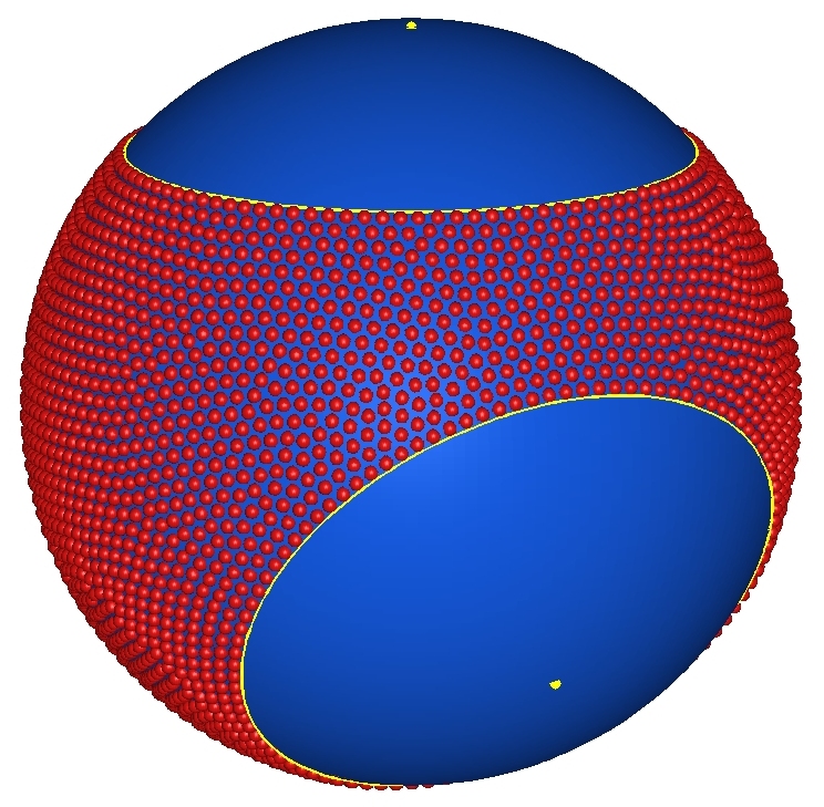
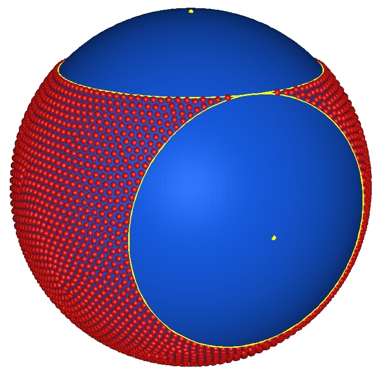
Figure 1: Approximate log-optimal points for $m=2$, $N=4000$ with $q_{1}=q_{2}=\frac{1}{4}$, $\mathbf{a}_{1}=(0,0,1)$ and $\mathbf{a}_{2}=(\frac{\sqrt{91}}{10},0,-\frac{3}{10})$ or $\mathbf{a}_{2}=(\frac{4\sqrt{5}}{9},0,-\frac{1}{9})$

Remark 4

Theorem 3.1 and Corollary 1 are illustrated in Figures 1 and 2 for two and three point sources, respectively. Observe, that the density of the (approximate) log-optimal configuration approaches the normalized surface area of the equilibrium support $S_{Q}=\Sigma_{\bm{\epsilon}}$.

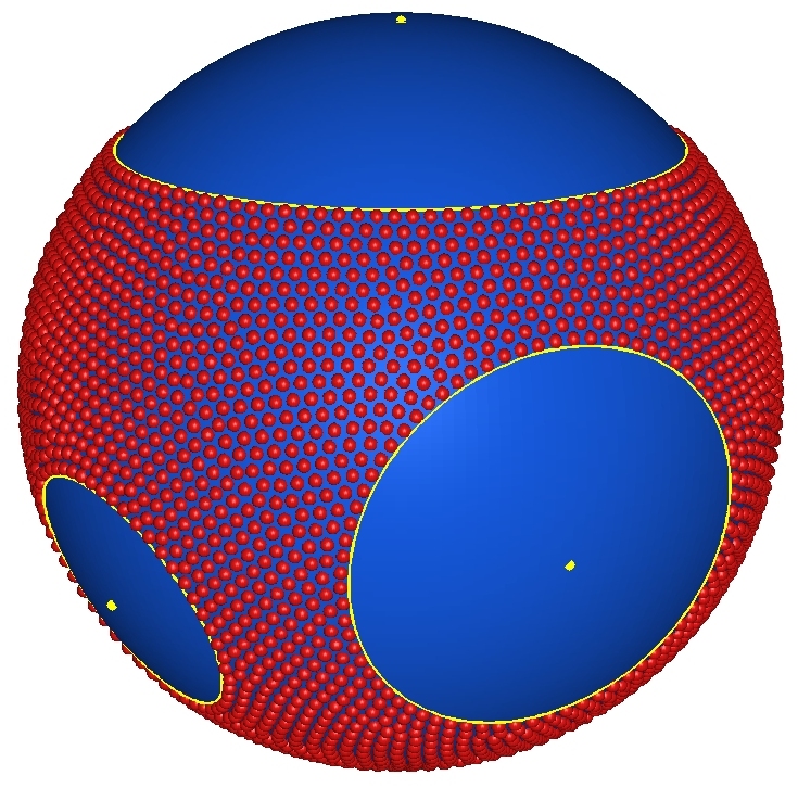
Figure 2: Approximate log-optimal points for $m=3$, $N=4000$ with $q_{1}=\frac{1}{4}$, $q_{2}=\frac{1}{8}$, $q_{3}=\frac{1}{20}$, $\mathbf{a}_{1}=(0,0,1)$, $\mathbf{a}_{2}=(\frac{\sqrt{91}}{10},0,-\frac{3}{10})$, and $\mathbf{a}_{3}=(0,\frac{\sqrt{3}}{2},-\frac{1}{2})$

Remark 5

The objective function for the optimization problem (7) with the discrete external field (13) is

$$E_{Q,N}(\mathbf{x}_{1},\ldots,\mathbf{x}_{N})=\sum_{1\leq i\neq j\leq N}k_{s}(\mathbf{x}_{i},\mathbf{x}_{j})+2(N-1)\sum_{i=1}^{m}q_{i}\sum_{j=1}^{N}k_{s_{i}}(\mathbf{a}_{i},\mathbf{x}_{j}),$$

where $k(\mathbf{x},\mathbf{y})$ is the Riesz kernel defined at he beginning of Section 1. The standard spherical parametrisation, $\mathbf{x}_{i}=(\sin(\theta_{i})\cos(\phi_{i})\;\sin(\theta_{i})\sin(\phi_{i})\;\cos(\theta_{i}))^{T}\in\mathbb{S}^{2}$ for $\theta_{i}\in[0,\pi]$ and $\phi_{i}\in[0,2\pi)$ is used to avoid the non-linear constraints $\mathbf{x}_{i}\cdot\mathbf{x}_{i}=1,i=1,\ldots,N$. This introduces singularities at the poles $\theta=0,\pi$, one of which can be avoided by using the rotational invariance of the objective function to place the first external field at the north pole. For $\theta_{i}\neq 0,\pi$ the gradient of $E_{Q,N}(\theta_{1},\phi_{1},\ldots,\theta_{N},\phi_{N})$ can be calculated for use in a nonlinear optimization method.

Point sets $\{\mathbf{x}_{1},\ldots,\mathbf{x}_{N}\}$ that provide approximate optimal s-energy configurations were obtained using this spherical parametrisation of the points and applying a nonlinear optimization method, for example a limited memory BFGS method for bound constrained problems ZhuByrLuNoc1997 , to find a local minimum of $E_{Q,N}$. The initial point sets $\{\mathbf{x}_{1},\ldots,\mathbf{x}_{N}\}$ used as starting points for the nonlinear optimization were uniformly distributed on $\mathbb{S}^{2}$, so did not reflect the structure of the external fields. A local perturbation of the point set achieving a local minimum was then used to generate a new starting point and the nonlinear optimization applied again. The best local minimizer found provided an approximation (upper bound) on the global minimum of $E_{Q,N}$. Different local minima arose from the fine structure of the points within their support.

The results above lend themselves to the following generalization. Given $m$ points $\mathbf{a}_{1},\dots,\mathbf{a}_{m}\in\mathbb{S}^{2}$, for each $i=1,\dots,m$ let $\phi_{i}$ be a radially-symmetric measure centered at $\mathbf{a}_{i}$ and supported on $\Sigma_{i,\rho_{i}}^{c}$ for some $\rho_{i}>0$ that has absolutely continuous density with respect to $\sigma_{2}$; i.e.,

$$\mathrm{d}\phi_{i}(\mathbf{x})=f_{i}(\langle\mathbf{x},\mathbf{a}_{i}\rangle)\,\mathrm{d}\sigma_{2}(\mathbf{x}),\qquad f_{i}(u)=0\quad\text{on $\bigg{[}-1,\sqrt{1-\rho_{i}^{2}/2}\bigg{]}$.}$$ (33)

Let $q_{i}:=\|\phi_{i}\|=\int\mathrm{d}\phi_{i}(\mathbf{x})$, $1\leq i\leq m$, and define the external field

$$Q_{\bm{\phi}}(\mathbf{x}):=\sum_{i=1}^{m}U_{0}^{\phi_{i}}(\mathbf{x})=\sum_{i=1}^{m}\int\log\frac{1}{|\mathbf{x}-\mathbf{a}_{i}|}\,\mathrm{d}\phi_{i}(\mathbf{x}),$$ (34)

where $\bm{\phi}=(\phi_{1},\dots,\phi_{m})$. Then the following theorem holds.

Theorem 3.2

Let $d=2$ and $s=0$. Let $Q_{\bm{\phi}}$ be defined by (34) and $\bm{\epsilon}$, $\Sigma_{\bm{\epsilon}}$ be defined by (20), (21). Suppose that $\Sigma_{i,\epsilon_{i}}^{c}\cap\Sigma_{j,\epsilon_{j}}^{c}=\emptyset$, $1\leq i<j\leq m$. Then the logarithmic extremal measure associated with $Q_{\bm{\phi}}$ is $\mu_{Q_{\bm{\phi}}}=\left(1+q\right){\sigma_{2}}_{|_{\Sigma_{\bm{\epsilon}}}}$ and the extremal support is $S_{Q_{\bm{\phi}}}=\Sigma_{\bm{\epsilon}}$.

Proof

The proof proceeds as in the proof of Theorem 3.1 with the adaption that the balayage measure of $\phi_{i}$ is given by

$$\widehat{\phi}_{i}=\operatorname{Bal}_{0}(\phi_{i},\Sigma_{i,\epsilon_{i}})=\|\phi\|\,\beta_{i}=q_{i}\,\beta_{i},$$

which follows easily from the hypothesis $\rho_{i}\leq\epsilon_{i}$ and the uniqueness of balayage measures.

We next formulate the analog of Theorem 3.1 in the complex plane $\mathbb{C}$. Let us fix one of the charges, say $\mathbf{a}_{m}$, at the North Pole $\mathbf{p}$, which will also serve as the center of the Kelvin transformation $\mathcal{K}$ (stereographic projection, or equivalently, inversion about the center $\mathbf{p}$) with radius $\sqrt{2}$ onto the equatorial plane. Set $w_{i}:=\mathcal{K}(\mathbf{a}_{i})$, $1\leq i\leq m$. The image of $\mathbf{a}_{m}$ under the Kelvin transformation is the ”point at infinity” in $\mathbb{C}$. Letting $z=\mathcal{K}(\mathbf{x})$, $\mathbf{x}\in\mathbb{S}^{2}$, we can utilize the following formulas

$$\left|\mathbf{x}-\mathbf{p}\right|=\frac{2}{\sqrt{1+|z|^{2}}},\qquad\left|\mathbf{x}-\mathbf{a}_{i}\right|=\frac{2|z-w_{i}|}{\sqrt{1+|z|^{2}}\,\sqrt{1+|w_{i}|^{2}}},\quad 1\leq i\leq m-1$$

to convert the continuous minimal energy problem (cf. (6)) and the discrete minimal energy problem (cf. (7)) on the sphere to their analog forms in the complex plane $\mathbb{C}$. Neglecting a constant term, we obtain in the complex plane the external field

$$\widetilde{Q}(z):=\sum_{i=1}^{m-1}q_{i}\log\frac{1}{|z-w_{i}|}+\left(1+q\right)\log\sqrt{1+|z|^{2}},\qquad z\in\mathbb{C}.$$ (35)

This external field is admissible in the sense of Saff-Totik SafTot1997 , since

$$\lim_{|z|\to\infty}\left(\widetilde{Q}(z)-\log|z|\right)=\lim_{|z|\to\infty}q_{m}\log|z|=\infty.$$

Therefore, there is a unique equilibrium measure $\mu_{\widetilde{Q}}$ characterized by variational inequalities similar to the ones in Proposition 1(d). The following theorem giving the extremal support $S_{\widetilde{Q}}$ and the extremal measure $\mu_{\widetilde{Q}}$ associated with the external field $\widetilde{Q}$ in (35) for sufficiently small $q_{i}$’s is a direct consequence of Theorem 3.1.

Theorem 3.3

Let $w_{1},\dots,w_{m-1}\in\mathbb{C}$ be fixed and $q_{1},\dots,q_{m}$ be positive real numbers with $q=q_{1}+\cdots+q_{m}$ and $\widetilde{Q}$ be the corresponding external field given in (35). Further, let $\mathbf{a}_{1},\dots,\mathbf{a}_{m-1}\in\mathbb{S}^{2}$ be the pre-images under the Kelvin transformation $\mathcal{K}$, i.e., $w_{i}=\mathcal{K}(\mathbf{a}_{i})$, $1\leq i\leq m-1$, and $a_{m}=\mathbf{p}$. If the $q_{i}$’s are sufficiently small so that $\Sigma_{i,\epsilon_{i}}^{c}\cap\Sigma_{j,\epsilon_{j}}^{c}=\emptyset$, $1\leq i<j\leq m$, where the spherical caps $\Sigma_{i,\epsilon_{i}}$ are defined in (21), then there are open discs $D_{1},\dots,D_{m-1}$ in $\mathbb{C}$ with $w_{i}\in D_{i}=\mathcal{K}(\Sigma_{i,\epsilon_{i}})$, $1\leq i\leq m-1$, such that

$$S_{\widetilde{Q}}=\left\{z\in\mathbb{C}\,:\,|z|\leq\sqrt{\frac{1+q-q_{m}}{q_{m}}}\right\}\setminus\bigcup_{i=1}^{m-1}D_{i}.$$ (36)

The extremal measure $\mu_{\widetilde{Q}}$ associated with $\widetilde{Q}$ is given by

$$\mathrm{d}\mu_{\widetilde{Q}}(z)=\frac{1+q}{\pi\left(1+|z|^{2}\right)^{2}}\,\mathrm{d}A(z),$$ (37)

where $\mathrm{d}A$ denotes the Lebesgue area measure in the complex plane.

Proof

The proof follows by a straight forward application of the Kelvin transformation to the weighted potential $U_{0}^{\mu_{Q}}(\mathbf{x})+Q(\mathbf{x})$ and using the identity relating the regular (not normalized) Lebesgue measure on the sphere and the area measure on the complex plane

$$\frac{4\pi}{\left|\mathbf{x}-\mathbf{p}\right|^{2}}\,\mathrm{d}\sigma_{2}(\mathbf{x})=\frac{1}{\left|z-\mathbf{p}\right|^{2}}\,\mathrm{d}A(z)$$

This change of variables yields the identity

$$U_{0}^{\mu_{Q}}(\mathbf{x})+Q(\mathbf{x})=U_{0}^{\mu_{\widetilde{Q}}}(z)+\widetilde{Q}(z)+const$$

from which, utilizing (31) and (32), one derives

$$U_{0}^{\mu_{\widetilde{Q}}}(z)+\widetilde{Q}(z) \geq C\quad\text{in $\mathbb{C}$,}$$ (38)

$$U_{0}^{\mu_{\widetilde{Q}}}(z)+\widetilde{Q}(z) =C\quad\text{on $S_{\widetilde{Q}}$,}$$ (39)

which implies that $\mu_{\widetilde{Q}}$ is the equilibrium measure by (SafTot1997, , Theorem 1.3).

Remark 6

At first it seems like a surprising fact that the equilibrium measure in Theorem 3.2 is uniform on $S_{Q}$ (i.e. has constant density). However, this can be easily seen alternatively from the planar version Theorem 3.3. Once we derive that the support $S_{\widetilde{Q}}$ is given by (36), we can recover the measure $\mu_{\widetilde{Q}}$ by applying Gauss’ theorem (cf. (SafTot1997, , Theorem II.1.3)), namely on any subregion of $S_{\widetilde{Q}}$ we have

$$d\mu_{\widetilde{Q}}=-\frac{1}{2\pi}\Delta U^{\mu_{\widetilde{Q}}}dA(z)=\frac{1}{2\pi}\Delta\widetilde{Q}(z)=\frac{1+q}{\pi(1+|z|^{2})^{2}}\,dA(z).$$

Recall that on this subregion $\log|z-w_{i}|$ is harmonic for all $i=1,\dots,m-1$. As $d\sigma_{2}(x)=dA(z)/[\pi(1+|z|^{2})^{2}]$, we get that $\mu_{Q}$ is the normalized Lebesgue surface measure on $S_{Q}$. Observe, that the same argument applies to the setting of Theorem 5.1 ($d=2,\ s=0$), from which we derive $\mu_{Q}=\left(1+q\right){\sigma_{2}}_{|_{S_{Q}}}$ even in the case when $\Sigma_{\epsilon_{i}}^{c}$ are not disjoint. Of course, we don’t know the equilibrium support $S_{Q}$ in this case. For related results see Bel2013 ; Bel2015 .

4 Riesz $(d-2)$-Energy Interactions on $\mathbb{S}^{d}$, $d\geq 3$

The case of $(d-2)$-energy interactions on $\mathbb{S}^{d}$, $d\geq 3$, and an external field $Q$ given by (13) is considerably more involved as the balayage measures utilized to determine the signed equilibrium on $\Sigma_{\bm{\gamma}}$ diminish their masses. This phenomenon yields an implicit nonlinear system for the critical values of the radii $\epsilon_{1},\dots,\epsilon_{m}$ (see (54) and (55)) characterizing the regions of electrostatic influence.

Let $d\geq 3$ and $0<d-2\leq s<d$. Let $\Phi_{s}(t_{i}):=\mathcal{F}_{s}(\Sigma_{i,\gamma_{i}})$ be the Mhaskar-Saff $\mathcal{F}$-functional associated with the external field $Q_{i}(\mathbf{x}):=q_{i}\,|\mathbf{x}-\mathbf{a}_{i}|^{-s}$ evaluated for the spherical cap $\Sigma_{i,\gamma_{i}}$. Then the signed $s$-equilibrium measure $\eta_{i,s}:=\eta_{\Sigma_{i,\gamma_{i}},Q_{i},s}$ on $\Sigma_{i,\gamma_{i}}$ associated with $Q_{i}$ is given by (see (BraDraSaf2009, , Theorem 11 and 15))

$$\eta_{i,s}=\frac{\Phi_{s}(t_{i})}{W_{s}(\mathbb{S}^{d})}\,\operatorname{Bal}_{s}(\sigma_{d},\Sigma_{i,\gamma_{i}})-q_{i}\,\operatorname{Bal}_{s}(\delta_{\mathbf{a}_{i}},\Sigma_{i,\gamma_{i}}).$$ (40)

For $d-2<s<d$ this signed measure is absolutely continuous

$$\mathrm{d}\eta_{i,s}(\mathbf{x})=\frac{\omega_{d-1}}{\omega_{d}}\eta_{i,s}^{\prime}(u)\left(1-u^{2}\right)^{d/2-1}\,\operatorname{\mathrm{d}}u\,\operatorname{\mathrm{d}}\sigma_{d-1}(\overline{\mathbf{x}}),\quad\mathbf{x}=(\sqrt{1-u^{2}}\,\overline{\mathbf{x}},u)\in\Sigma_{i,\gamma_{i}},$$

with density function

$$\begin{split}\eta_{i,s}^{\prime}(u)&=\frac{1}{W_{s}(\mathbb{S}^{d})}\frac{\operatorname{\Gamma}(d/2)}{\operatorname{\Gamma}(d-s/2)}\left(\frac{1-t_{i}}{1-u}\right)^{d/2}\left(\frac{t_{i}-u}{1-t_{i}}\right)^{(s-d)/2}\\ &\phantom{=\times}\times\Bigg{\{}\Phi_{s}(t_{i})\,{\sideset{{}_{2}}{{}_{1}}{\operatorname{\mathop{\mathbf{F}\/}\nolimits\!}}\!\left(\begin{subarray}{c}\displaystyle 1,d/2\\ \displaystyle 1-(d-s)/2\end{subarray};\frac{t_{i}-u}{1-u}\right)}-\frac{q_{i}\,2^{d-s}}{{\gamma_{i}}^{d}}\Bigg{\}}.\end{split}$$ (41)

For the ratio $\frac{\omega_{d-1}}{\omega_{d}}$ see (4), a formula for the Riesz $s$-energy $W_{0}(\mathbb{S}^{d})$ is given in (1), and ${}_{2}\operatorname{\mathop{\mathbf{F}\/}\nolimits\!}_{1}$ denotes Olver’s regularized ${}_{2}F_{1}$-hypergeometric function (NIST:DLMF, , Eq. 15.2.2). For $s=d-2$ the signed $(d-2)$-equilibrium

$$\eta_{i,d-2}=\frac{\Phi_{d-2}(t_{i})}{W_{d-2}(\mathbb{S}^{d})}{\sigma_{d}}_{|_{\Sigma_{i,\gamma_{i}}}}+\frac{1-t_{i}}{2}\left(1-t_{i}^{2}\right)^{d/2-1}\left[\Phi_{d-2}(t_{i})-\frac{4q_{i}}{\gamma_{i}^{d}}\right]\beta_{i}$$ (42)

has, like in the logarithmic case (see (22)), a boundary-supported component $\beta_{i}$, which is the normalized Lebesgue measure on the boundary circle of $\Sigma_{i,\gamma}$. Observe that in either case the signed equilibrium has a negative component if and only if

$$\Phi_{s}(t_{i})-\frac{2^{d-s}q_{i}}{\gamma_{i}^{d}}<0,\qquad\text{where $2(1-t_{i})=\gamma_{i}^{2}$.}$$ (43)

The weighted $s$-potential of $\eta_{i,s}$, $d-2<s<d$, satisfies ((BraDraSaf2009, , Theorem 11))

$$U_{s}^{\eta_{i,s}}(\mathbf{z})+Q_{i}(\mathbf{z}) =\Phi_{s}(t_{i}),\qquad\mathbf{z}\in\Sigma_{i,\gamma_{i}},$$ (44)

$$\begin{split}U_{s}^{\eta_{i,s}}(\mathbf{z})+Q_{i}(\mathbf{z})&=\Phi_{s}(t_{i})+\frac{q_{i}}{[2(1-\xi_{i})]^{s/2}}\,\operatorname{I}\Bigg{(}\frac{2}{1-t_{i}}\frac{\xi_{i}-t_{i}}{1+\xi_{i}};\frac{d-s}{2},\frac{s}{2}\Bigg{)}\\ &\phantom{=\pm}-\Phi_{s}(t_{i})\,\operatorname{I}\Bigg{(}\frac{\xi_{i}-t_{i}}{1+\xi_{i}};\frac{d-s}{2},\frac{s}{2}\Bigg{)},\qquad\mathbf{z}\in\mathbb{S}^{d}\setminus\Sigma_{i,\gamma_{i}},\end{split}$$ (45)

where $\mathbf{z}=(\sqrt{1-\xi_{i}^{2}}\;\overline{\mathbf{z}},\xi_{i})\in\mathbb{S}^{d}$, $-1\leq\xi_{i}\leq 1$ and $\overline{\mathbf{z}}\in\mathbb{S}^{d-1}$, and

$$\operatorname{I}(x;a,b):=\frac{\operatorname{B}(x;a,b)}{\operatorname{B}(a,b)},\quad\operatorname{B}(a,b):=\operatorname{B}(1;a,b),\quad\operatorname{B}(x;a,b):=\int_{0}^{x}u^{a-1}(1-u)^{b-1}\,du$$

are the regularized incomplete beta function, the beta function, and the incomplete beta function (NIST:DLMF, , Ch. 5 and 8); whereas ((BraDraSaf2009, , Lemmas 33 and 36))

$$U_{d-2}^{\eta_{i,d-2}}(\mathbf{z})+Q_{i}(\mathbf{z}) =\Phi_{d-2}(t_{i}),\qquad\mathbf{z}\in\Sigma_{i,\gamma_{i}},$$ (46)

$$\begin{split}U_{d-2}^{\eta_{i,d-2}}(\mathbf{z})+Q_{i}(\mathbf{z})&=\Phi_{d-2}(t_{i})\left(\frac{1+t_{i}}{1+\xi_{i}}\right)^{d/2-1}+\frac{q_{i}}{\left(2(1-\xi_{i})\right)^{d/2-1}}\\ &\phantom{=\pm}-\frac{q_{i}}{\gamma_{i}^{d-2}}\left(\frac{1+t_{i}}{1+\xi_{i}}\right)^{d/2-1},\qquad\mathbf{z}\in\mathbb{S}^{d}\setminus\Sigma_{i,\gamma_{i}}.\end{split}$$ (47)

The last relation follow from (45) if $s$ is changed to $d-2$.

In the proof of our main result for $s=d-2$, $d\geq 3$, we need the analog of (31), which we derive from a similar result for the weighted potential (45). As this is of independent interest, we state and prove the following lemma for $d-2\leq s<d$.

Lemma 1

Let $d\geq 3$ and $d-2\leq s<d$. If (43) is satisfied, then the weighted $s$-potential of the signed $s$-equilibrium $\eta_{i,s}$ satisfies the variational inequalities

$$U_{s}^{\eta_{i,s}}(\mathbf{z})+Q_{i}(\mathbf{z}) =\Phi_{s}(t_{i}),\qquad\mathbf{z}\in\Sigma_{i,\gamma_{i}},$$ (48)

$$U_{s}^{\eta_{i,s}}(\mathbf{z})+Q_{i}(\mathbf{z}) >\Phi_{s}(t_{i}),\qquad\mathbf{z}\in\mathbb{S}^{d}\setminus\Sigma_{i,\gamma_{i}}.$$ (49)

Furthermore, both relations remain valid if equality is allowed in (43).

Proof

The first equality (48) was established in (BraDraSaf2009, , Theorems 11 and 15).

Let $d\geq 3$ and $d-2\leq s<d$. The right-hand side of (45) is a function of $\xi_{i}$ with $t_{i}<\xi_{i}\leq 1$. We denote it by $G(\xi_{i})$. Using the integral form of the incomplete regularized beta function, we get

$$\begin{split}\operatorname{B}\Big{(}\frac{d-s}{2},\frac{s}{2}\Big{)}\,\Big{(}G(\xi_{i})-\Phi_{s}(t_{i})\Big{)}&=\left(\frac{1-t_{i}}{1-\xi_{i}}\right)^{s/2}\frac{2^{d-s}q_{i}}{\gamma_{i}^{d}}\int_{0}^{\frac{\xi_{i}-t_{i}}{1+\xi_{i}}}u^{\frac{d-s}{2}-1}\left(1-\frac{2\,u}{1-t_{i}}\right)^{\frac{s}{2}-1}\operatorname{\mathrm{d}}u\\ &\phantom{=}-\Phi_{s}(t_{i})\int_{0}^{\frac{\xi_{i}-t_{i}}{1+\xi_{i}}}u^{\frac{d-s}{2}-1}\left(1-u\right)^{\frac{s}{2}-1}\operatorname{\mathrm{d}}u.\end{split}$$

Let (43) be satisfied. Then

$$\begin{split}\operatorname{B}\Big{(}\frac{d-s}{2},\frac{s}{2}\Big{)}\,\frac{G(\xi_{i})-\Phi_{s}(t_{i})}{\Phi_{s}(t_{i})}&>\left[\frac{1-t_{i}}{1-\xi_{i}}\right]^{s/2}\int_{0}^{\frac{\xi_{i}-t_{i}}{1+\xi_{i}}}u^{\frac{d-s}{2}-1}\left(1-\frac{2}{1-t_{i}}\,u\right)^{\frac{s}{2}-1}\operatorname{\mathrm{d}}u\\ &\phantom{=}-\int_{0}^{\frac{\xi_{i}-t_{i}}{1+\xi_{i}}}u^{\frac{d-s}{2}-1}\left(1-u\right)^{\frac{s}{2}-1}\operatorname{\mathrm{d}}u.\end{split}$$

The square-bracketed expression is $>1$ for $-1<t_{i}<\xi_{i}\leq 1$. Since ${\frac{2}{1-t_{i}}>1}$, the first integrand is bounded from below by the second integrand if $\frac{s}{2}-1\leq 0$. In the case $\frac{s}{2}-1>0$, we observe that for $0\leq u\leq\frac{\xi_{i}-t_{i}}{1+\xi_{i}}$,

$$\begin{split}\left[\frac{1-t_{i}}{1-\xi_{i}}\right]^{s/2}\left(1-\frac{2}{1-t_{i}}\,u\right)^{\frac{s}{2}-1}&=\frac{1-t_{i}}{1-\xi_{i}}\left(\frac{1-t_{i}}{1-\xi_{i}}-\frac{2}{1-\xi_{i}}\,u\right)^{\frac{s}{2}-1}\\ &>\left(\frac{1-t_{i}}{1-\xi_{i}}-\frac{2}{1-\xi_{i}}\,u\right)^{\frac{s}{2}-1}\\ &\geq\left(1-u\right)^{\frac{s}{2}-1}.\end{split}$$

The estimates are strict in both cases. Hence, equality is allowed in (43).

We are now ready to state and prove the second main result.

Theorem 4.1

Let $d\geq 3$ and $s=d-2$. Let $Q$ be defined by (13). Suppose the positive charges $q_{1},\dots,q_{m}$ are sufficiently small. Then there exists a critical $\bm{\epsilon}=(\epsilon_{1},\dots,\epsilon_{m})$, uniquely defined by these charges, such that $\Sigma_{\epsilon_{i}}^{c}\cap\Sigma_{\epsilon_{j}}^{c}=\emptyset$, $1\leq i<j\leq m$, and the $(d-2)$-extremal measure associated with $Q$ is $\mu_{Q}=C\,{\sigma_{d}}_{|_{\Sigma_{\bm{\epsilon}}}}$ for a uniquely defined normalization constant $C>1$ and the extremal support is $S_{Q}=\Sigma_{\bm{\epsilon}}$.

Furthermore, an optimal $(d-2)$-energy $N$-point configuration w.r.t. $Q$ is contained in $S_{Q}$ for every $N\geq 2$.

Proof

Let $\bm{\gamma}=(\gamma_{1},\dots,\gamma_{m})$ be a vector of $m$ positive numbers such that ${\Sigma_{i,\gamma_{i}}^{c}\cap\Sigma_{i,\gamma_{j}}^{c}=\emptyset}$, $1\leq i<j\leq m$. We consider the signed measure

$$\tau:=C\,\operatorname{Bal}_{d-2}(\sigma_{d},\Sigma_{\bm{\gamma}})-\operatorname{Bal}_{d-2}(q_{1}\,\delta_{\mathbf{a}_{1}}+\cdots+q_{m}\,\delta_{\mathbf{a}_{m}},\Sigma_{\bm{\gamma}}).$$

As balayage under Riesz $(d-2)$-kernel interactions satisfies (16), we have

$$U_{d-2}^{\tau}(\mathbf{z})+Q(\mathbf{z}) =C\,U_{d-2}^{\sigma_{d}}(\mathbf{z})=C\,W_{d-2}(\mathbb{S}^{d}), \mathbf{z} \in\Sigma_{\bm{\gamma}},$$

$$U_{d-2}^{\tau}(\mathbf{z})+Q(\mathbf{z}) \geq C\,U_{d-2}^{\operatorname{Bal}_{d-2}(\sigma_{d},\Sigma_{\bm{\gamma}})}(\mathbf{z}), \mathbf{z} \in\mathbb{S}^{d}\setminus\Sigma_{\bm{\gamma}}.$$

If the normalization constant $C=C(\bm{\gamma})$ is chosen such that $\|\tau\|=\tau(\Sigma_{\bm{\gamma}})=1$, then $\tau$ is a signed $(d-2)$-equilibrium measure on $\Sigma_{\bm{\gamma}}$ associated with $Q$ and, by uniqueness, $\eta_{\Sigma_{\bm{\gamma}},Q}=\tau$ and $F_{\Sigma_{\bm{\gamma}},Q}=\mathcal{F}_{s}(\Sigma_{\bm{\gamma}})$ with $C=\mathcal{F}_{s}(\Sigma_{\bm{\gamma}})/W_{d-2}(\mathbb{S}^{d})$.

We show the variational inequality for $\mathbf{z}\in\mathbb{S}^{d}\setminus\Sigma_{\bm{\gamma}}$ and proceed in a similar fashion as in the proof of Theorem 3.1. For $i=1,\ldots,m$ let

$$\nu_{i}:={\sigma_{d}}_{|_{\Sigma_{i,\gamma_{i}}^{c}}},\qquad\widehat{\nu_{i}}:=\operatorname{Bal}_{d-2}(\nu_{i},\Sigma_{i,\gamma_{i}}),\qquad\widehat{\delta_{\mathbf{a}_{i}}}:=\operatorname{Bal}_{d-2}(\delta_{\mathbf{a}_{i}},\Sigma_{i,\gamma_{i}}),$$ (50)

where $t_{i}$ is the projection of the boundary circle $\partial\Sigma_{i,\gamma_{i}}$ onto the $\mathbf{a}_{i}$-axis; recall that $2(1-t_{i})=\gamma_{i}^{2}$. As the open spherical caps $\Sigma_{i,\gamma_{i}}^{c}$, $1\leq i\leq m$, do not intersect for $i\neq j$, we have $\partial\Sigma_{\gamma_{i}}\subset\partial\Sigma_{\bm{\gamma}}$. Balayage in steps yields

$$\operatorname{Bal}_{d-2}(\nu_{i},\Sigma_{\bm{\gamma}}) =\operatorname{Bal}_{d-2}(\nu_{i},\Sigma_{i,\gamma_{i}})=\widehat{\nu_{i}}=W_{d-2}(\mathbb{S}^{d})\,\frac{1-t_{i}}{2}\left(1-t_{i}^{2}\right)^{d/2-1}\beta_{i},$$

$$\operatorname{Bal}_{d-2}(\delta_{\mathbf{a}_{i}},\Sigma_{\bm{\gamma}}) =\operatorname{Bal}_{d-2}(\delta_{\mathbf{a}_{i}},\Sigma_{i,\gamma_{i}})=\widehat{\delta_{\mathbf{a}_{i}}}=\frac{4}{\gamma_{i}^{d}}\,\frac{1-t_{i}}{2}\left(1-t_{i}^{2}\right)^{d/2-1}\beta_{i},$$

where the respective last step follow from (BraDraSaf2009, , Lemmas 33 and 36) and it is crucial that $\widehat{\nu_{i}}$ and $\widehat{\delta_{\mathbf{a}_{i}}}$ are supported on $\partial\Sigma_{i,\gamma_{i}}$ and thus $\partial\Sigma_{\bm{\gamma}}$, so that

$$\tau =C\,{\sigma_{d}}_{|_{\Sigma_{\bm{\gamma}}}}+C\,\sum_{i=1}^{m}\widehat{\nu}_{i}-\sum_{i=1}^{m}q_{i}\,\widehat{\delta_{\mathbf{a}_{i}}}$$ (51)

$$=C\,{\sigma_{d}}_{|_{\Sigma_{\bm{\gamma}}}}+\sum_{i=1}^{m}\left(C\,W_{d-2}(\mathbb{S}^{d})-\frac{4q_{i}}{\gamma_{i}^{d}}\right)\frac{1-t_{i}}{2}\left(1-t_{i}^{2}\right)^{d/2-1}\beta_{i}.$$ (52)

Observe, the signed measure $\tau$ has a negative component if and only if

$$C\,W_{d-2}(\mathbb{S}^{d})-\frac{4q_{i}}{\gamma_{i}^{d}}<0\qquad\text{for at least one $i\in\{1,\dots,m\}$.}$$

Let $\mathbf{z}\in\mathbb{S}^{d}\setminus\Sigma_{\bm{\gamma}}$. Then $\mathbf{z}\in\Sigma_{i_{0},\gamma_{i_{0}}}^{c}$ for some $i_{0}\in\{1,\dots,m\}$ and $\mathbf{z}\in\Sigma_{i,\gamma_{i}}$ for all $i\neq i_{0}$. Hence,

$$U_{d-2}^{\tau}(\mathbf{z})+Q(\mathbf{z})=C\,W_{d-2}(\mathbb{S}^{d})+C\left(U_{d-2}^{\widehat{\nu_{i_{0}}}}(\mathbf{z})-U_{d-2}^{\nu_{i_{0}}}(\mathbf{z})\right)-q_{i_{0}}\left(U_{d-2}^{\widehat{\delta_{\mathbf{a}_{i_{0}}}}}(\mathbf{z})-U_{d-2}^{\delta_{\mathbf{a}_{i_{0}}}}(\mathbf{z})\right).$$

Using (19), from (BraDraSaf2009, , Lemmas 33)

$$U_{d-2}^{\widehat{\nu_{i_{0}}}}(\mathbf{z})-U_{d-2}^{\nu_{i_{0}}}(\mathbf{z})=W_{d-2}(\mathbb{S}^{d})\left(\frac{1+t_{i_{0}}}{1+\xi_{i_{0}}}\right)^{d/2-1}-W_{d-2}(\mathbb{S}^{d})<0$$

and from (BraDraSaf2009, , Lemmas 36),

$$U_{d-2}^{\widehat{\delta_{\mathbf{a}_{i_{0}}}}}(\mathbf{z})-U_{d-2}^{\delta_{\mathbf{a}_{i_{0}}}}(\mathbf{z})=\frac{1}{\gamma_{i_{0}}^{d-2}}\left(\frac{1+t_{i_{0}}}{1+\xi_{i_{0}}}\right)^{d/2-1}-\frac{1}{\left(2(1-\xi_{i_{0}})\right)^{d/2-1}}<0;$$

hence

$$\begin{split}U_{d-2}^{\tau}(\mathbf{z})+Q(\mathbf{z})&=C\,W_{d-2}(\mathbb{S}^{d})\left(\frac{1+t_{i_{0}}}{1+\xi_{i_{0}}}\right)^{d/2-1}-\frac{q_{i_{0}}}{\gamma_{i_{0}}^{d-2}}\left(\frac{1+t_{i_{0}}}{1+\xi_{i_{0}}}\right)^{d/2-1}\\ &\phantom{=}+\frac{q_{i_{0}}}{\left(2(1-\xi_{i_{0}})\right)^{d/2-1}}.\end{split}$$

Observe the similarity to (47). Essentially the same argument as in the proof of Lemma 1 shows that

$$U_{d-2}^{\tau}(\mathbf{z})+Q(\mathbf{z})>C\,W_{d-2}(\mathbb{S}^{d}),\qquad\mathbf{z}\in\Sigma_{i_{0},\gamma_{i_{0}}}$$

in the case when

$$C\,W_{d-2}(\mathbb{S}^{d})-\frac{4q_{i_{0}}}{\gamma_{i_{0}}^{d}}\leq 0,\qquad i=1,\dots,m.$$ (53)

It is not difficult to see that near $\partial\Sigma_{i_{0},\gamma_{i_{0}}}$ the following asymptotics holds:

$$\begin{split}U_{d-2}^{\tau}(\mathbf{z})+Q(\mathbf{z})&=C\,W_{d-2}(\mathbb{S}^{d})+\left(\frac{d}{2}-1\right)\left(\frac{4q_{i_{0}}}{\gamma_{i_{0}}^{d}}-C\,W_{0}(\mathbb{S}^{d})\right)\frac{\xi_{i_{0}}-t_{i_{0}}}{1+t_{i_{0}}}\\ &\phantom{=C\,W_{d-2}(\mathbb{S}^{d})}+\frac{1}{2}\left(\frac{d}{2}-1\right)\frac{d}{2}\left(\frac{4q_{i_{0}}}{\gamma_{i_{0}}^{d}}\frac{2t_{i_{0}}}{1+t_{i_{0}}}+C\,W_{0}(\mathbb{S}^{d})\right)\left(\frac{\xi_{i_{0}}-t_{i_{0}}}{1+t_{i_{0}}}\right)^{2}\\ &\phantom{=C\,W_{d-2}(\mathbb{S}^{d})}+\mathcal{O}\Big{(}\left(\frac{\xi_{i_{0}}-t_{i_{0}}}{1+t_{i_{0}}}\right)^{3}\Big{)}\qquad\text{as $\xi_{i_{0}}\to t_{i_{0}}^{+}$;}\end{split}$$

i.e., the weighted $(d-2)$-potential of $\tau$ will be negative sufficiently close to $\partial\Sigma_{i_{0},\gamma_{i_{0}}}$ if (53) does not hold. Hence, if the necessary conditions (53) are satisfied, then

$$U_{d-2}^{\tau}(\mathbf{z})+Q(\mathbf{z})>C\,W_{d-2}(\mathbb{S}^{d}),\qquad\mathbf{z}\in\Sigma_{\bm{\gamma}}^{c}.$$

Suppose, the system

$$C\,W_{d-2}(\mathbb{S}^{d}) =\frac{4q_{i}}{\gamma_{i}^{d}},\qquad i=1,\dots,m,$$ (54)

$$C\,\sigma_{d}(\Sigma_{\bm{\gamma}}) =1,$$ (55)

subject to the geometric side conditions

$$\Sigma_{i,\gamma_{i}}\bigcap\Sigma_{j,\gamma_{j}}=\emptyset,\qquad 1\leq i<j\leq m,$$ (56)

has a solution $(\bm{\gamma},C)$ with $\bm{\gamma}=\bm{\gamma}(C)\in(0,2)^{m}$ and $C>0$, then $\eta_{\Sigma_{\bm{\gamma}},Q}=\tau=C\,{\sigma_{d}}_{|_{\Sigma_{\bm{\gamma}}}}$ with $F_{\Sigma_{\bm{\gamma}},Q}=C\,W_{d-2}(\mathbb{S}^{d})$ satisfies the variational inequalities

$$\begin{split}U_{d-2}^{\eta_{\Sigma_{\bm{\gamma}},Q}}(\mathbf{z})+Q(\mathbf{z})&=F_{\Sigma_{\bm{\gamma}},Q},\qquad\mathbf{z}\in\Sigma_{\bm{\gamma}},\\ U_{d-2}^{\eta_{\Sigma_{\bm{\gamma}},Q}}(\mathbf{z})+Q(\mathbf{z})&>F_{\Sigma_{\bm{\gamma}},Q},\qquad\mathbf{z}\in\Sigma_{\bm{\gamma}}^{c},\end{split}$$ (57)

and thus, by Proposition 1(d), $\mu_{Q}=\eta_{\Sigma_{\bm{\gamma}},Q}=C\,{\sigma_{d}}_{|_{\Sigma_{\bm{\gamma}}}}$ and $S_{Q}=\Sigma_{\bm{\gamma}}$. Observe that, given a collection of pairwise different points $\mathbf{a}_{1},\dots,\mathbf{a}_{m}\in\mathbb{S}^{d}$, for sufficiently small charges $q_{1},\dots,q_{m}$, there always exists such a solution. In particular, this is the case if (55) holds for $\gamma_{i}=[4q_{i}/W_{d-2}(\mathbb{S}^{d})]^{1/d}$.

To determine the parameter $C$, denote $g(C):=C\sigma_{d}(\Sigma_{\bm{\gamma}})$, where

$$\gamma_{i}:=\gamma_{i}(C)=\left[\frac{4q_{i}}{CW_{d-2}(\mathbb{S}^{d})}\right]^{1/d},\qquad i=1,\dots,m.$$

As $\gamma_{i}=\gamma_{i}(C)$ are decreasing and continuous functions for all $i=1,\dots,m$, we derive that $\sigma_{d}(\Sigma_{\bm{\gamma}})$ is an increasing and continuous function of $C$ and so is $g(C)$. Also, note that $g(1)=\sigma_{d}(\Sigma_{\bm{\gamma}})<1$, and $\lim_{C\to\infty}g(C)=\infty$. Therefore, there exists a unique solution $C^{*}$ of the equation

$$C\sigma_{d}\left(\bigcap_{i=1}^{m}\Sigma_{i,\gamma_{i}}\right)=1,$$

where the $\gamma_{i}$’s are defined by (54).

Finally, we invoke (BraDraSaf2014, , Corollary 13) and (57) to conclude that an optimal $(d-2)$-energy $N$-point configuration w.r.t. $Q$ is contained in $S_{Q}$.

5 Regions of Electrostatic Influence and Optimal $(d-2)$-Energy Points

In this section we consider what happens when the regions of electrostatic influence (see Remark 3 after Theorem 3.1) have intersecting interiors. We are going to utilize the techniques in the proofs of (BraDraSaf2014, , Theorem 14 and Corollary 15) to show that the support of the $(d-2)$-equilibrium measure associated with the external field (13) satisfies $S_{Q}\subset\Sigma_{\bm{\epsilon}}$, and hence the optimal $(d-2)$-energy points stay away from $\Sigma_{\bm{\epsilon}}^{c}$. We are going to a prove our result for $s$ in the range $d-2\leq s<d$.

Let $\mathbf{a}_{1},\dots,\mathbf{a}_{m}\in\mathbb{S}^{d}$ be $m$ fixed points with associated positive charges $q_{1},\dots,q_{m}$. We define for $d-2\leq s<d$ the external field

$$Q_{s}(\mathbf{x}):=\sum_{i=1}^{m}q_{i}\,k_{s}(\mathbf{a}_{i},\mathbf{x}),\qquad\mathbf{x}\in\mathbb{S}^{d}.$$ (58)

We introduce the reduced charges

$$\overline{q}_{i}:=\frac{q_{i}}{1+q-q_{i}},\qquad 1\leq i\leq m.$$

Let $\overline{\Phi}_{s}(t_{i})$ be the Mhaskar-Saff $\mathcal{F}_{s}$-functional associated with the external field $\overline{q}_{i}\,k_{s}(\mathbf{a}_{i},\bm{\cdot})$ evaluated for the spherical cap $\Sigma_{i,\gamma_{i}}$ (cf. Section 4) where it is used that $t_{i}$ and $\gamma_{i}$ are related by $2(1-t_{i})=\gamma_{i}^{2}$. Let $\overline{\gamma}_{i}$ denote the unique solution of the equation

$$\overline{\Phi}_{s}(t_{i})=\frac{2^{d-s}\overline{q}_{i}}{\gamma_{i}^{d}},\qquad 1\leq i\leq m.$$ (59)

Theorem 5.1

Let $d-2\leq s<d$, $d\geq 2$, and let $\overline{\bm{\gamma}}=(\overline{\gamma}_{1},\dots,\overline{\gamma}_{m})$ be the vector of solutions of (59). Then the support $S_{Q_{s}}$ of the $s$-extremal measure $\mu_{Q_{s}}$ associated with the external field $Q_{s}$ defined in (58) is contained in the set $\Sigma_{\overline{\bm{\gamma}}}=\bigcap_{i=1}^{m}\Sigma_{i,\overline{\gamma}_{i}}$. If $d=2$ and $s=0$, then $\overline{\gamma}_{i}=\epsilon_{i}$, $1\leq i\leq m$, where $\epsilon_{i}$ is defined in (20).

Furthermore, no point of an optimal $N$-point configuration w.r.t. $Q_{s}$ lies in $\Sigma_{i,\overline{\gamma}_{i}}$, $1\leq i\leq m$.

Proof

First, we consider the case $d-2<s<d$. Let $i$ be fixed. Since the external field (58) has a singularity at $\mathbf{a}_{i}$, it is true that $S_{Q_{s}}\subset\Sigma_{i,\rho}$ for some $\rho>0$. Moreover, as noted after Definition 2, $S_{Q_{s}}\subset\operatorname{supp}(\eta_{\Sigma_{i,\gamma},Q_{s}}^{+})$ for all $\gamma$ such that $S_{Q_{s}}\subset\Sigma_{i,\gamma}$. It is easy to see that the signed equilibrium on $\Sigma_{i,\gamma}$ associated with $Q_{s}$ is given by

$$\eta_{\Sigma_{i,\gamma},Q_{s}}=\frac{1+\sum_{j=1}^{m}q_{j}\,\|\widehat{\delta_{\mathbf{a}_{j}}}\|}{\|\widehat{\nu_{i}}\|}\,\widehat{\nu_{i}}-\sum_{j=1}^{m}q_{j}\,\widehat{\delta_{\mathbf{a}_{j}}},$$ (60)

where

$$\widehat{\nu_{i}}=\operatorname{Bal}_{s}(\sigma_{d},\Sigma_{i,\gamma}),\qquad\widehat{\delta_{\mathbf{a}_{j}}}=\operatorname{Bal}_{s}(\delta_{\mathbf{a}_{j}},\Sigma_{i,\gamma}).$$

Observe, that if $\mathbf{a}_{j}\in\Sigma_{i,\gamma}$ then $\widehat{\delta_{\mathbf{a}_{j}}}=\delta_{\mathbf{a}_{j}}$. We will show that for all $\rho<\gamma<\overline{\gamma}_{i}$ the signed $s$-equilibrium measure in (60) will be negative near the boundary $\partial\Sigma_{i,\gamma}$. Indeed, with the convention that the inequality between two signed measures ${\nu_{1}\leq\nu_{2}}$ means that ${\nu_{2}-\nu_{1}}$ is a non-negative measure, we have

$$\eta_{\Sigma_{i,\gamma},Q_{s}} \leq\frac{1+\sum_{j=1}^{m}q_{j}\,\|\widehat{\delta_{\mathbf{a}_{j}}}\|}{\|\widehat{\nu_{i}}\|}\,\widehat{\nu_{i}}-q_{i}\,\widehat{\delta_{\mathbf{a}_{i}}}$$

$$\leq\left(1+q-q_{i}\right)\left(\frac{1+\overline{q}_{i}\,\|\widehat{\delta_{\mathbf{a}_{i}}}\|}{\|\widehat{\nu_{i}}\|}\,\widehat{\nu_{i}}-\overline{q}_{i}\,\widehat{\delta_{\mathbf{a}_{i}}}\right)$$

$$=\left(1+q-q_{i}\right)\left[\frac{\overline{\Phi}_{s}(t)}{W_{s}(\mathbb{S}^{d})}\widehat{\nu_{i}}-\overline{q}_{i}\,\widehat{\delta_{\mathbf{a}_{i}}}\right],$$ (61)

where $2(1-t)=\gamma^{2}$. The square-bracketed part is the signed equilibrium measure on $\Sigma_{i,\gamma}$ associated with the external field $\overline{q}_{i}\,k_{s}(\mathbf{a}_{i},\bm{\cdot})$ and has a negative component near the boundary $\partial\Sigma_{i,\gamma}$ if and only if $\overline{\Phi}_{s}(t)-\frac{2^{d-s}\overline{q}_{i}}{\gamma^{d}}<0$ as noted after (42). This inequality holds whenever $\rho<\gamma<\overline{\gamma}_{i}$ and the inclusion relation $S_{Q_{s}}\subset\Sigma_{i,\gamma}$ for all $\rho<\gamma<\overline{\gamma}_{i}$ can now be easily deduced. As $i$ was arbitrarily fixed, we derive $S_{Q_{s}}\subset\Sigma_{\overline{\bm{\gamma}}}$. As an optimal $N$-point configuration w.r.t. $Q_{s}$ is confined to $S_{Q_{s}}$, no point of such a configuration lies in $\Sigma_{i,\overline{\gamma}_{i}}^{c}$, $1\leq i\leq m$.

In order to obtain the result of the theorem for $d=2$ and $s=0$, we use that balayage under logarithmic interaction preserves mass. Hence

$$\eta_{\Sigma_{i,\gamma},Q_{0}}=\overline{\Phi}_{0}(t)\,\widehat{\nu_{i}}-\sum_{j=1}^{m}q_{j}\,\widehat{\delta_{\mathbf{a}_{j}}}\leq\overline{\Phi}_{0}(t)\,\widehat{\nu_{i}}-\overline{q}_{i}\,\widehat{\delta_{\mathbf{a}_{i}}},\qquad\overline{\Phi}_{0}(t):=1+q$$

and the characteristic equation $\overline{\Phi}_{0}(t)=\frac{4\overline{q}_{i}}{\overline{\gamma}^{2}}$ reduces to $\overline{\gamma}^{2}=\frac{4\overline{q}_{i}}{1+\overline{q}_{i}}$. As before, no point of an optimal $N$-point configuration w.r.t. $Q_{0}$ lies in $\Sigma_{i,\overline{\gamma}_{i}}^{c}$, $1\leq i\leq m$. This completes the proof.

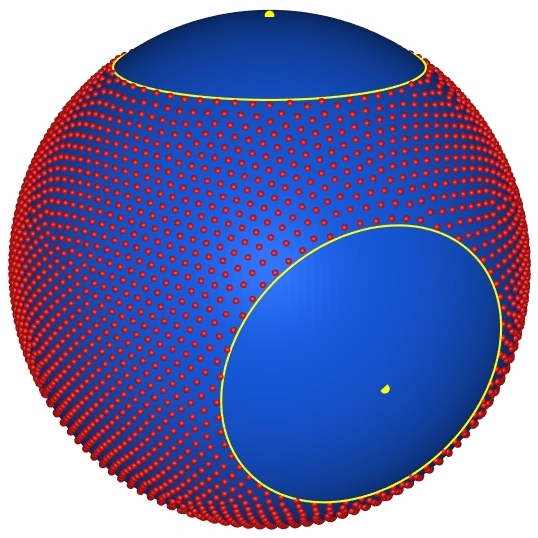
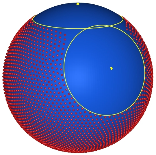
Figure 3: Approximate Coulomb-optimal points for $m=2$, $N=4000$, $q_{1}=q_{2}=\frac{1}{4}$, $\mathbf{a}_{1}=(0,0,1)$ and $\mathbf{a}_{2}=(0,\frac{\sqrt{91}}{10},-\frac{3}{10})$ or $\mathbf{a}_{2}=(0,\frac{\sqrt{91}}{10},\frac{3}{10})$

Example 1

Observe, that if the charges $q_{1},\dots,q_{m}$ are selected sufficiently small so that for all $i$ we have $\mathbf{a}_{j}\in\Sigma_{\gamma_{i}}$, then close to the boundary $\partial\Sigma_{\gamma_{i}}$ equality holds in (61). So, the critical $\gamma_{i}$ can be determined by solving the equation

$$\overline{\Phi}_{s}(t_{i})-2^{d-s}\overline{q}_{i}/\gamma_{i}^{d}=0,$$

where

$$\overline{\Phi}_{s}(t_{i})=W_{s}(\mathbb{S}^{d})\frac{1+\overline{q}_{i}\|\widehat{\delta}_{t_{i},s}\|}{\|\operatorname{Bal}_{s}(\sigma_{2},\Sigma_{\gamma_{i}})\|}.$$ (62)

Motivated by this, we consider the important case of Coulomb interaction potential, namely when $d=2$ and $s=1$. We find that (see (BraDraSaf2009, , Lemmas 29 and 30))

$$W_{1}(\mathbb{S}^{2})=1,\quad\|\widehat{\delta}_{t_{i},1}\|=\frac{\arcsin t_{i}}{\pi}+\frac{1}{2},\quad\|\operatorname{Bal}_{s}(\sigma_{2},\Sigma_{\gamma_{i}})\|=\frac{\sqrt{1-t_{i}^{2}}+\arcsin t_{i}}{\pi}+\frac{1}{2}.$$

Maximizing the Mhaskar-Saff $\mathcal{F}_{1}$-functional $\overline{\Phi}_{1}(t)$ is equivalent to solving the equation

$$\frac{\pi(1+\overline{q}_{i}/2)+\overline{q}_{i}\arcsin t_{i}}{\sqrt{1-t_{i}^{2}}+\arcsin t_{i}+\pi/2}=\frac{\overline{q}_{i}}{1-t_{i}}.$$

An equivalent equation in term of the geodesic radius $\alpha_{i}$ of the cap $\Sigma_{\epsilon_{i}}^{c}$ of electrostatic influence, so $t_{i}=\cos(\alpha_{i})$ is

$$({\bar{q}}_{i}+1)\pi\cos(\alpha)-{\bar{q}}_{i}\alpha\cos(\alpha)+{\bar{q}}_{i}\sin(\alpha)-\pi=0.$$

Problem 1

The two images in Figure 4 compare approximate log-optimal configurations with $4000$ and $8000$ points. The two yellow circles are the boundaries of $\Sigma_{1,\epsilon_{1}}$ and $\Sigma_{2,\epsilon_{2}}$. It is evident that optimal log-energy points stay away from the caps of electrostatic influence $\Sigma_{1,\epsilon_{1}}^{c}$ and $\Sigma_{2,\epsilon_{2}}^{c}$ of the two charges. In the limit, the log-optimal points approach the log-equilibrium support, which seems to be a smooth region excluding these caps of electrostatic influence. We conclude this section by posing as an open problem, the precise determination of the support in such a case.

Figure 4: Approximate log-optimal points for $m=2$, $N=4000$ (left) and $N=8000$ (right), $q_{1}=q_{2}=\frac{1}{4}$, $\mathbf{a}_{1}=(0,0,1)$, $\mathbf{a}_{2}=(\frac{\sqrt{91}}{10},0,\frac{3}{10})$

References

• (1) Beltrán, C.: Harmonic properties of the logarithmic potential and the computability of elliptic Fekete points. Constr. Approx. 37(1), 135–165 (2013). DOI 10.1007/s00365-012-9158-y. URL http://dx.doi.org/10.1007/s00365-012-9158-y
• (2) Beltrán, C.: A facility location formulation for stable polynomials and elliptic Fekete points. Found. Comput. Math. 15(1), 125–157 (2015). DOI 10.1007/s10208-014-9213-0. URL http://dx.doi.org/10.1007/s10208-014-9213-0
• (3) Bilogliadov, M.: Weighted energy problem on the unit sphere. Anal. Math. Phys. 6(4), 403–424 (2016). DOI 10.1007/s13324-016-0125-9. URL http://dx.doi.org/10.1007/s13324-016-0125-9
• (4) Brauchart, J.S., Dragnev, P.D., Saff, E.B.: Riesz extremal measures on the sphere for axis-supported external fields. J. Math. Anal. Appl. 356(2), 769–792 (2009). DOI 10.1016/j.jmaa.2009.03.060. URL http://dx.doi.org/10.1016/j.jmaa.2009.03.060
• (5) Brauchart, J.S., Dragnev, P.D., Saff, E.B.: Riesz external field problems on the hypersphere and optimal point separation. Potential Anal. 41(3), 647–678 (2014). DOI 10.1007/s11118-014-9387-8. URL http://dx.doi.org/10.1007/s11118-014-9387-8
• (6) NIST Digital Library of Mathematical Functions. http://dlmf.nist.gov/, Release 1.0.15 of 2017-06-01. URL http://dlmf.nist.gov/. F. W. J. Olver, A. B. Olde Daalhuis, D. W. Lozier, B. I. Schneider, R. F. Boisvert, C. W. Clark, B. R. Miller and B. V. Saunders, eds.
• (7) Dragnev, P.D., Saff, E.B.: Riesz spherical potentials with external fields and minimal energy points separation. Potential Anal. 26(2), 139–162 (2007). DOI 10.1007/s11118-006-9032-2. URL http://dx.doi.org/10.1007/s11118-006-9032-2
• (8) Landkof, N.S.: Foundations of modern potential theory. Springer-Verlag, New York-Heidelberg (1972). Translated from the Russian by A. P. Doohovskoy, Die Grundlehren der mathematischen Wissenschaften, Band 180
• (9) Le Gia, Q.T., Sloan, I.H., Wendland, H.: Multiscale approximation for functions in arbitrary Sobolev spaces by scaled radial basis functions on the unit sphere. Appl. Comput. Harmon. Anal. 32(3), 401–412 (2012). DOI 10.1016/j.acha.2011.07.007. URL http://dx.doi.org/10.1016/j.acha.2011.07.007
• (10) Le Gia, Q.T., Sloan, I.H., Wendland, H.: Multiscale RBF collocation for solving PDEs on spheres. Numer. Math. 121(1), 99–125 (2012). DOI 10.1007/s00211-011-0428-6. URL http://dx.doi.org/10.1007/s00211-011-0428-6
• (11) Mhaskar, H.N., Saff, E.B.: Where does the sup norm of a weighted polynomial live? (A generalization of incomplete polynomials). Constr. Approx. 1(1), 71–91 (1985). DOI 10.1007/BF01890023. URL http://dx.doi.org/10.1007/BF01890023
• (12) Saff, E.B., Totik, V.: Logarithmic potentials with external fields, Grundlehren der Mathematischen Wissenschaften [Fundamental Principles of Mathematical Sciences], vol. 316. Springer-Verlag, Berlin (1997). DOI 10.1007/978-3-662-03329-6. URL http://dx.doi.org/10.1007/978-3-662-03329-6. Appendix B by Thomas Bloom
• (13) Zhu, C., Byrd, R.H., Lu, P., Nocedal, J.: Algorithm 778: L-BFGS-B: Fortran subroutines for large-scale bound-constrained optimization. ACM Trans. Math. Software 23(4), 550–560 (1997). DOI 10.1145/279232.279236. URL http://dx.doi.org/10.1145/279232.279236
• (14) Zoriĭ, N.V.: Equilibrium potentials with external fields. Ukraïn. Mat. Zh. 55(9), 1178–1195 (2003). DOI 10.1023/B:UKMA.0000018005.67743.86. URL http://dx.doi.org/10.1023/B:UKMA.0000018005.67743.86