Keyring models: an approach to steerability

Carl A. Miller National Institute of Standards and Technology, 100 Bureau Dr., Gaithersburg, MD 20899, USA Joint Center for Quantum Information and Computer Science, University of Maryland, College Park, MD 20742, USA camiller@umd.edu    Roger Colbeck Department of Mathematics, University of York, York, YO10 5DD, UK roger.colbeck@york.ac.uk    Yaoyun Shi Aliyun Quantum Laboratory, Alibaba USA, Bellevue, WA 98004, USA y.shi@alibaba-inc.com
($9^{\mathrm{th}}$ February 2018)
Abstract

If a measurement is made on one half of a bipartite system, then, conditioned on the outcome, the other half has a new reduced state. If these reduced states defy classical explanation—that is, if shared randomness cannot produce these reduced states for all possible measurements—the bipartite state is said to be steerable. Determining which states are steerable is a challenging problem even for low dimensions. In the case of two-qubit systems a criterion is known for $T$-states (that is, those with maximally mixed marginals) under projective measurements. In the current work we introduce the concept of keyring models—a special class of local hidden state models. When the measurements made correspond to real projectors, these allow us to study steerability beyond $T$-states.

Using keyring models, we completely solve the steering problem for real projective measurements when the state arises from mixing a pure two-qubit state with uniform noise. We also give a partial solution in the case when the uniform noise is replaced by independent depolarizing channels.

I Introduction

In his 1964 paper Bell John Bell made the fundamental observation that measurement correlations exhibited by some entangled quantum states cannot be explained by any local causal model. Specifically, if $\rho_{AB}$ is the state of a bipartite system shared by Alice and Bob, and Alice is given a private input $q\in\mathcal{Q}$ and Bob is given a private input $s\in\mathcal{S}$, then it is possible for Alice and Bob to measure $\rho_{AB}$ and produce output messages $a\in\mathcal{A}$ and $b\in\mathcal{B}$ such that the conditional probability distribution $\mathbf{P}(ab\mid qs)$ cannot be simulated by any local hidden variable (LHV) model.

This can be interpreted as a fundamental confirmation of the models for nonlocality used in quantum physics, and it also has important applications in information processing. Device-independent quantum cryptography is based on the observation that if two untrusted input-output devices exhibit nonlocal correlations, their internal processes must be quantum. With correctly chosen protocols and mathematical proof, this observation allows a classical user to manipulate the devices to perform cryptographic tasks and at the same time verify their security Mayers:1998 ; BHK .

In 2007, the related notion of quantum steering was distilled Wiseman:2007 , in which, rather than having Bob make a measurement, we directly consider the subnormalized marginal states $\tilde{\rho}_{B}^{\,q,a}$ that he holds when Alice receives input $q$ and produces output $a$. A local hidden state (LHS) model attempts to generate these using shared randomness. Denoting the shared randomness by a random variable $\lambda$, distributed according to probability distribution $\mu(\lambda)$, Bob can output quantum state $\sigma_{\lambda}$, while Alice outputs $a$ according to a probability distribution $\mathbf{P}_{q,\lambda}(a)$.

Suppose when Alice gets input $q$ she performs a POVM $\{E^{q}_{a}\}_{a\in\mathcal{A}}$, so that $\tilde{\rho}_{B}^{\,q,a}={\rm Tr}_{A}((E^{q}_{a}\otimes\mathbb{I}_{B})\rho_{AB})$. A LHS model produces a faithful simulation if $\tilde{\rho}_{B}^{\,q,a}=\int_{\lambda}\mathbf{P}_{q,\lambda}(a)\sigma_{\lambda}\ \mathrm{d}\mu(\lambda)$ for all $q$ and $a$. If such a model exists, then we say that the state $\rho_{AB}$ is unsteerable for the family of measurements $\{\{E^{q}_{a}\}_{a\in\mathcal{A}}\}_{q\in\mathcal{Q}}$. If a LHS model exists for all possible measurements Alice could do (i.e., all POVMs), we say $\rho_{AB}$ is unsteerable. Conversely, if there exists a set of measurements for which no LHS model exists, then $\rho_{AB}$ is said to be steerable.

One can think of steering as an analog of non-locality for the case where one party (Bob) trusts his measurement device (and hence in principle could do tomography to determine his marginal state after being told Alice’s measurement and outcome). It is hence a useful intermediate between entanglement witnessing (both measurement devices trusted) and Bell violations (neither trusted) and has applications such as one-sided device-independent quantum cryptography Branciard:2012 and (sub)channel discrimination Piani:2015 . Exhibiting new steerable states offers an expanded toolbox for such problems.

The steering decision problem is to determine whether or not a given state is steerable. This problem has proved to be difficult even for $2$-qubit systems. To understand why this is so, consider a two-qubit state $\rho_{AB}$. If Alice were to measure $\{{|0\rangle\!\langle 0|},{|1\rangle\!\langle 1|}\}$ on input $q=0$ and $\{{|+\rangle\!\langle+|},{|-\rangle\!\langle-|}\}$ on input $q=1$ (where $|\pm\rangle=(|0\rangle\pm|1\rangle)/\sqrt{2}$), then it is possible for Bob to obtain one of four subnormalized states which we denote $\tilde{\rho}_{B}^{\,0},\tilde{\rho}_{B}^{\,1},\tilde{\rho}_{B}^{\,+},\tilde{\rho}_{B}^{\,-}$ (where, for example, $\tilde{\rho}_{B}^{\,0}={\rm Tr}_{A}[({|0\rangle\!\langle 0|}\otimes\mathbb{I}_{B})\rho]$). Determining whether a LHS model exists for these four states is a search over a finite-dimensional space and is not difficult (see Cavalcanti ; Hirsch for techniques for searching for LHS models). Next suppose Alice additionally performs the measurement $\{{|\pi/4\rangle\!\langle\pi/4|},{|5\pi/4\rangle\!\langle 5\pi/4|}\}$ for input $q=2$, where

$$|\theta\rangle:=\cos\frac{\theta}{2}|0\rangle+\sin\frac{\theta}{2}|1\rangle\,,$$ (1)

leading to states $\tilde{\rho}_{B}^{\,\pi/4},\tilde{\rho}_{B}^{\,5\pi/4}$. There is no guarantee that a local hidden state model that simulates the previous four states will simulate this new pair as well (generally, the states $\tilde{\rho}_{B}^{\,\pi/8},\tilde{\rho}_{B}^{\,5\pi/8}$ are not in the convex hull of the former states). A new search for local hidden state models is required, and the search space increases exponentially with each new measurement. Thus a direct approach—even when just dealing with measurements of the form $\{{|\theta\rangle\!\langle\theta|},{|\theta+\pi\rangle\!\langle\theta+\pi|}\}$—is unlikely to be feasible.

Previous work on steering has achieved success by exploiting the symmetries of certain classes of states. For the class of Werner states Werner $\left\{\rho_{AB}(\eta)\mid\eta\in[0,1]\right\}$ given by

$\displaystyle\rho_{AB}(\eta)$ $\displaystyle=$ $\displaystyle\eta{|\Phi_{+}\rangle\!\langle\Phi_{+}|}+(1-\eta)\mathbb{I}/4,$ (2)

where $|\Phi_{+}\rangle=\frac{1}{\sqrt{2}}(|00\rangle+|11\rangle)$, an exact classification of $P$-steerability (i.e., steerability for all projective measurements) has been performed (see Appendix A for a summary of results on Werner states). More recently a complete classification of $P$-steerability for $T$-states (i.e., states for which $\rho_{A}$ and $\rho_{B}$ are maximally mixed) has been given Jevtic:2015 ; Nguyen:PRA ; Nguyen:2016 . [Note that the requirement on $\rho_{B}$ can be dropped—see Lemma 16 below.] In both cases the methods depend critically on the symmetry of the states. For $2$-qubit states outside the family of $T$-states, partial results on steerability exist (e.g., Jones07 ; Bowles:2016 ) but a full classification is not known.

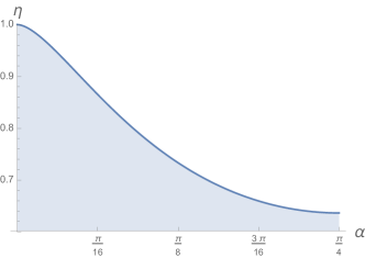
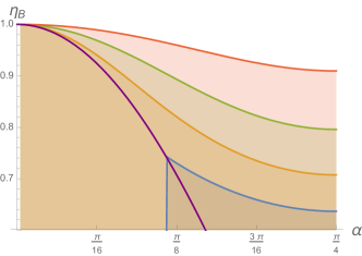
In the current work, we develop new techniques to decide steerability in the case where $\rho_{A}$ is not maximally mixed. We study Real Projective (RP)-steerability (i.e., steerability by the family of all measurements of the form $\{{|\theta\rangle\!\langle\theta|},{|\theta+\pi\rangle\!\langle\theta+\pi|}\}$) for real two-qubit states. [A state is real if its matrix elements are real in the $\{|0\rangle,|1\rangle\}$ basis.] To illustrate our techniques, we give a complete classification of RP-steerability for the class of states, $\left\{\rho_{AB}(\alpha,\eta)\right\}$, formed by mixing partially entangled pure states with uniform noise, i.e.,

$\displaystyle\rho_{AB}(\alpha,\eta)=\eta{|\phi_{\alpha}\rangle\!\langle\phi_{\alpha}|}+(1-\eta)\mathbb{I}/4\,,$ (3)

where $|\phi_{\alpha}\rangle=\cos\alpha|00\rangle+\sin\alpha|11\rangle$. The classification is shown in Figure 1, where the shaded/unshaded region represents the states that are unsteerable/steerable for real projective measurements. As a special case we recover the existing result Jones11 ; Uola16 that Werner states are RP-steerable if and only if $\eta>2/\pi$ (see Theorem 17).

Our criterion also applies to a larger class of real $2$-qubit states, specifically, all states whose steering ellipse is tilted at an angle less than $\pi/4$—see Theorem 14 and Corollary 15 for the formal statements. To achieve this classification we introduce the concept of keyring models, which are a geometrically motivated class of local hidden state models for one-dimensional families of measurements. We explain these in more detail in the next subsection.

Our approach invites generalizations. In its current form we have a criterion for steerability among all real $2$-qubit states whose steering ellipse is tilted at an angle less than $\pi/4$. With additional work one may be able to go further identify the set of all $RP$-steerable real $2$-qubit states. Additionally, the keyring approach could be applied in more general scenarios where steering is attempted with any one-dimensional family of measurements.

Refer to caption
Figure 1: $RP$-unsteerability for the states $\rho_{AB}(\alpha,\eta)$. In the shaded region the states are unsteerable under real projective measurements, while above it they are steerable. (Note that the shaded region extends to $\eta=0$.)

Studying the behavior of qubit states under real projective measurements is a natural problem for experimental setups in which measurements in one plane of the Bloch sphere are easier than the most general measurements. However, another future goal would be to extend our methods to arbitrary complex measurements on $2$-qubit states. This looks more challenging—steering with a $2$-dimensional family of measurements is considerably harder than with a $1$-dimensional family of measurements—but if it can be accomplished, it would be an important step towards a complete criterion for steering among arbitrary $2$-qubit states.

Keyring models can also be used to construct a class of LHV models if we also use a (classical) function on Bob’s side to map his input and the hidden state to his output. They can hence be applied to the related problem of classically simulating bipartite correlations and may, for example, be useful for shedding new light on the problem of identifying the smallest detector efficiency for observing Bell inequality violations. We hope to find further applications of keyring models in this direction.

I.1 Sketch of the proof techniques

The difficulty in establishing steerability over all measurements is the need to rule out all LHS models. Our proof begins with the observation that, in the case where $\rho_{AB}$ is a real $2$-qubit state and where the set of measurements comprises real projective measurements (i.e., those of the form $\{{|\theta\rangle\!\langle\theta|},{|\theta+\pi\rangle\!\langle\theta+\pi|}\}$), a more tractable (though still infinite dimensional) class of LHS models suffices. Specifically, we consider a class of LHS models that we call “keyring models”, which we now define.
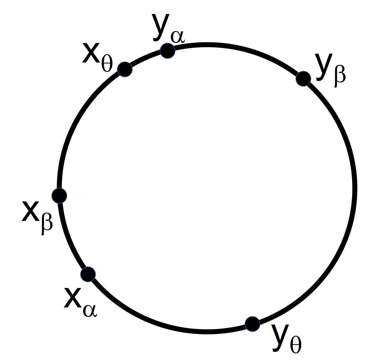
Let $\mathbb{RP}^{1}$ denote the set of all real one-dimensional projectors on $\mathbb{C}^{2}$ (i.e., the set $\{{|\theta\rangle\!\langle\theta|}\}_{\theta\in[0,2\pi)}$). A keyring model is a pair $(\mu,\{f_{\theta}\}_{\theta})$, where $\mu$ is a probability distribution on $\mathbb{RP}^{1}$, and $f_{\theta}\colon\mathbb{RP}^{1}\to[0,1]$ is a two-step function—that is, roughly speaking, a function that takes two possible values and switches between them at two elements of $\mathbb{RP}^{1}$ (see Definition 4). The word “keyring” refers to the configuration of the two switching points on $\mathbb{RP}^{1}$ as $\theta$ varies. An example configuration is shown in Figure 2. (This definition is related to the local hidden state models of Jones11 ; Jevtic:2015 ; Nguyen:PRA ; Nguyen:2016 , which are based on functions on $\mathbb{RP}^{2}$ that are supported on half-spheres. One key difference in the definition of a keyring model is that there is no uniformity in the positioning of the switching points of the functions $f_{\theta}$—they need not be diametrically opposite.)

Refer to caption
Figure 2: An example configuration of endpoints in a keyring distribution. For every point in $\mathbb{RP}^{1}$ there are two associated endpoints in $\mathbb{RP}^{1}$. Here three pairs of endpoints are illustrated with $(x_{\alpha},y_{\alpha})$ being the end points for $\alpha$, for example.

We show that $\rho_{AB}$ is RP-steerable if and only if it can be simulated by a keyring model. Denoting the subnormalized reduced states on Bob’s side by $\tilde{\rho}_{B}(\theta)={\rm Tr}_{A}\left(({|\theta\rangle\!\langle\theta|}\otimes\mathbb{I}_{B})\rho_{AB}\right)$, this is equivalent to the requirement

$\displaystyle\tilde{\rho}_{B}(\theta)$ $\displaystyle=$ $\displaystyle\int_{x\in\mathbb{RP}^{1}}xf_{\theta}(x)\ \mathrm{d}\mu$ (4)

for all $\theta$. From this we can conclude that that if the circumference of the steering ellipse $\{\tilde{\rho}_{B}(\theta)\}$ is greater than $2$, i.e.,

$\displaystyle\int_{\mathbb{RP}^{1}}\left\|\frac{\mathrm{d}}{\mathrm{d}\theta}\tilde{\rho}_{B}(\theta)\right\|_{1}\mathrm{d}\theta$ $\displaystyle>$ $\displaystyle 2,$ (5)

where $\|\cdot\|_{1}$ is the trace norm, then the state $\rho_{AB}$ has no local hidden state model (see Proposition 6).

At this point our proof diverges from that of Jones11 ; Jevtic:2015 ; Nguyen:PRA ; Nguyen:2016 , since the converse of the above statement is not true in our case: if (5) fails to hold, there could still be no local hidden state model. However, the following stronger condition guarantees the existence of a local hidden state model:

$\displaystyle\int_{\mathbb{RP}^{1}}\left|\frac{\mathrm{d}}{\mathrm{d}\theta}\tilde{\rho}_{B}(\theta)\right|\mathrm{d}\theta$ $\displaystyle\leq$ $\displaystyle 2\rho_{B},$ (6)

where $|X|=\sqrt{X^{\dagger}X}$ is the absolute value of the operator. Moreover, the state $\rho_{AB}$ is steerable if and only if

$\displaystyle\rho^{\prime}_{AB}:=(\mathbb{I}_{A}\otimes Y)\rho_{AB}(\mathbb{I}_{A}\otimes Y)$ (7)

is steerable for all positive definite $Y$ (see Lemma 16), and by substituting in $\rho^{\prime}_{AB}$ for $\rho_{AB}$ in (5) and (6) we obtain an infinite family of criteria for $RP$-steerability and $RP$-unsteerability. We thus need to find a $Y$ such that one of (5) and (6) holds for $\rho^{\prime}_{AB}$.

The most technically difficult part of our proof then shows that there must exist a positive definite density matrix $Y$ such that

$\displaystyle Y^{-1}\left[\int_{\mathbb{RP}^{1}}\left|Y\left(\frac{\mathrm{d}}{\mathrm{d}\theta}\tilde{\rho}_{B}(\theta)\right)Y\right|\mathrm{d}\theta\right]Y^{-1}$ (8)

is a scalar multiple of $\rho_{B}$. This compels (8) to either be greater than, or less than or equal to $\rho_{B}$, and thus we achieve a criterion for steering which is both necessary and sufficient. We prove this by demonstrating that if we let $Y$ tend to any projector $P$ in $\mathbb{RP}^{1}$, then (8) must tend to an operator proportional to the orthogonal projector $\widehat{P}$. Any continuous map from a $2$-dimensional disc to itself which rotates the boundary of the disc must be an onto map, and this gives the desired result. (The proof of the aforementioned limit assertion is surprisingly subtle—it turns out that the rate at which the normalization of (8) approaches $\widehat{P}$ is only logarithmic.)

Theorem 14 gives a formal statement of our main result. To apply the criteria (e.g., to obtain Figure 1), we use numerical computations to find the appropriate operators $Y$ from a given state $\rho_{AB}$.

II Preliminaries

II.1 Notation and Definitions

For any Hilbert space $\mathcal{H}$, let $\mathcal{A}(\mathcal{H})$ denote the set of all Hermitian operators on $\mathcal{H}$, $\mathcal{P}_{\geq}(\mathcal{H})$ be the set of positive semidefinite operators on $\mathcal{H}$, $\mathcal{P}_{>}(\mathcal{H})$ be the set of positive definite operators on $\mathcal{H}$, $\mathcal{D}(\mathcal{H})$ denote the set of all density operators on $\mathcal{H}$, and $\mathcal{D}_{>}(\mathcal{H})$ denote the set of all positive definite density operators on $\mathcal{H}$. Let $\mathcal{RA}(\mathcal{H}),\mathcal{RP}_{\geq}(\mathcal{H})$ etc. denote the respective subsets of real operators (an operator $X$ is real if $\langle i|X|j\rangle\in\mathbb{R}$ for all $i,j$, where $\{|i\rangle\}$ is the standard basis). If $A,B\in\mathcal{P}_{\geq}(\mathcal{H})$ we write $A\geq B$ to mean that $A-B\in\mathcal{P}_{\geq}(\mathcal{H})$ and $A\ngeq B$ for the complement of this. For an operator $X$ on $\mathcal{H}$ we use $|X|:=\sqrt{X^{\dagger}X}$ and $\|X\|_{1}:={\rm Tr}|X|$, the latter being the trace norm of $X$. If ${\rm Tr}(X)\neq 0$, we use $\left<X\right>$ to denote the normalized version of $X$, i.e., $\left<X\right>:=X/{\rm Tr}(X)$. In addition, if $Y$ is also an operator on $\mathcal{H}$, then we use $\langle X,Y\rangle:={\rm Tr}(X^{\dagger}Y)$.

Throughout this paper, we take $\mathcal{H}_{A}=\mathcal{H}_{B}=\mathbb{C}^{2}$ to be qubit systems possessed by Alice and Bob and use $\mathbb{RP}^{1}\subseteq\mathcal{RD}(\mathcal{H})$ to denote the set of one-dimensional real projectors on $\mathbb{C}^{2}$.

II.1.1 The steering ellipse

Any operator $\lambda\in\mathcal{RA}(\mathbb{C}^{2})$ can be expressed uniquely in terms of real numbers $n$, $r_{1}$, $r_{3}$ as

$\displaystyle\lambda=\frac{1}{2}(n\mathbb{I}+r_{1}\sigma_{1}+r_{3}\sigma_{3})\,,$ (9)

where $\sigma_{1}=|0\rangle\!\langle 1|+|1\rangle\!\langle 0|$ and $\sigma_{3}={|0\rangle\!\langle 0|}-{|1\rangle\!\langle 1|}$ are the usual Pauli operators. Note that $\lambda\in\mathbb{RP}^{1}$ if and only if $n=1$ and $r_{1}^{2}+r_{3}^{2}=1$.

The tilt of $\lambda$, denoted ${\rm Tilt}(\lambda)$, is the quantity $\sqrt{r^{2}_{1}+r^{2}_{3}}/|n|$ (if $n=0$, the tilt is $\infty$). The tilt angle of $\lambda$ is $\arctan({\rm Tilt}(\lambda))$. If we think of $(n,r_{1},r_{3})$ as $3$-dimensional Cartesian coordinates, then the tilt angle of $\lambda$ is angle that it forms with the $(1,0,0)$ axis. We use these coordinates when we sketch steering ellipses later in this work. Note that an operator is positive semidefinite if and only if $n\geq 0$ and its tilt is less than or equal to $1$. It is useful to note that

$$\|\lambda\|_{1}=\left\{\begin{array}[]{ll}|n|&\text{if }{\rm Tilt}(\lambda)\leq 1\\ \sqrt{r_{1}^{2}+r_{3}^{2}}&\text{if }{\rm Tilt}(\lambda)>1\end{array}\right.$$ (10)

Let $\rho_{AB}\in\mathcal{RD}(\mathbb{C}^{2}\otimes\mathbb{C}^{2})$. Then, the steering ellipse of $\rho_{AB}$ on $B$ is the function $\tilde{\rho}_{B}\colon\mathbb{RP}^{1}\to\mathcal{P}_{\geq}(\mathbb{C}^{2})$ given by

$\displaystyle\tilde{\rho}_{B}(\theta)$ $\displaystyle:=$ $\displaystyle{\rm Tr}_{A}\left[\left({|\theta\rangle\!\langle\theta|}\otimes\mathbb{I}_{B}\right)\rho_{AB}\right]\,,$ (11)

where $|\theta\rangle$ is defined in (1). Note that $\{|\theta\rangle,|\theta+\pi\rangle\}$ form an orthonormal basis, so $\rho_{B}=\tilde{\rho}_{B}(\theta)+\tilde{\rho}_{B}(\theta+\pi)$ for any $\theta$. (In the more general case of arbitrary projective measurements, the states on Bob’s side are a two-parameter family that define an ellipsoid rather than an ellipse. Note also that the term “steering ellipsoid” is used to refer to the set of normalized states in the literature JPJR ; Jevtic:2015 , while our steering ellipse comprises subnormalized states).

Definition 1.

Let $\rho_{AB}\in\mathcal{RD}(\mathbb{C}^{2}\otimes\mathbb{C}^{2})$. Then, the tilt of the steering ellipse of $\rho_{AB}$ is the equal to the tilt of any nonzero vector that is normal to the $2$-dimensional affine space that contains the steering ellipse of $\rho_{AB}$. [If the steering ellipse does not span a $2$-dimensional affine space (i.e., it is degenerate) then we say that its tilt is equal to $\infty$.]

Note that if the tilt of the steering ellipse is less than or equal to $1$, then no element of the steering ellipse is strictly greater (in the positive semidefinite sense) than any other. This is a consequence of Lemma 20 in the appendix.

II.1.2 Local hidden state models

In this section we give a definition of a local hidden state model. It is not the most general definition possible, but it suffices for our purposes because of the form of the steering problem we are considering, as we now explain.

In the most general sense, a local hidden state model for a set of real $2$-qubit subnormalized states $\left\{\tilde{\rho}_{B}^{\,q,a}\right\}_{q\in\mathcal{Q},a\in\mathcal{A}}$ is a probability distribution $\mu$ on $\mathcal{D}(\mathbb{C}^{2})$ and set of functions $\left\{f_{q,a}\colon\mathcal{D}(\mathbb{C}^{2})\to[0,1]\right\}_{q,a}$ with $\sum_{a\in\mathcal{A}}f_{q,a}(x)=1$ such that

$\displaystyle\tilde{\rho}_{B}^{\,q,a}$ $\displaystyle=$ $\displaystyle\int_{x\in\mathcal{D}(\mathbb{C}^{2})}xf_{q,a}(x)\ \mathrm{d}\mu\,.$ (12)

(To connect with the earlier description, $f_{q,a}(x)$ is the probability that Alice gives the outcome $a$ for measurement $q$ when the hidden variable takes the value $x$.) However, via the map $\mathcal{D}(\mathbb{C}^{2})\to\mathcal{RD}(\mathbb{C}^{2})$ given by $x\mapsto(x+\overline{x})/2$, we may assume $\mu,f_{a,q}$ have support $\mathcal{RD}(\mathbb{C}^{2})$, and by decomposing each operator in $\mathcal{RD}(\mathbb{C}^{2})$ into a convex combination of one-dimensional projectors, we may further assume that $\mu,f_{q,a}$ have support $\mathbb{RP}^{1}$. We are thus led to the following definition.

Definition 2.

A local hidden state model for a set $\left\{\tilde{\rho}_{B}^{\,q,a}\right\}_{q\in\mathcal{Q},a\in\mathcal{A}}\subseteq\mathcal{RP}_{\geq}(\mathbb{C}^{2})$ is a pair $(\mu,\{f_{q,a}\}_{q,a})$ such that $\mu$ is a probability distribution on $\mathbb{RP}^{1}$, $f_{q,a}\colon\mathbb{RP}^{1}\to[0,1]$ with $\sum_{a\in\mathcal{A}}f_{q,a}(x)=1$ for all $q$, and

$\displaystyle\tilde{\rho}_{B}^{\,q,a}$ $\displaystyle=$ $\displaystyle\int_{x\in\mathbb{RP}^{1}}xf_{q,a}(x)\ \mathrm{d}\mu\,.$ (13)

In the case of steering for real 2-qubit states under real projective measurements, it suffices to consider whether we can find $(\mu,\{f_{\theta}\}_{\theta})$ with $f_{\theta}\colon\mathbb{RP}^{1}\to[0,1]$ such that

$$\tilde{\rho}_{B}(\theta)=\int_{x\in\mathbb{RP}^{1}}xf_{\theta}(x)\ \mathrm{d}\mu\,.$$ (14)

(Here $f_{\theta}(x)$ is the probability that Alice gives the outcome corresponding to the first projector for the measurement $\{{|\theta\rangle\!\langle\theta|},{|\theta+\pi\rangle\!\langle\theta+\pi|}\}$ when the hidden variable has value $x$.) If such a $(\mu,\{f_{\theta}\}_{\theta})$ can be found, this constitutes a LHS model for the set $\{\tilde{\rho}_{B}(\theta)\}_{\theta\in[0,2\pi)}$ and we say that $\rho_{AB}$ is RP-unsteerable. Conversely, if no such model exists, we say that $\rho_{AB}$ is RP-steerable.

Remark 3.

The property of having a LHS model is convex, i.e., if $\rho_{AB}$ and $\rho^{\prime}_{AB}$ have LHS models (for some set of measurements), then so does $p\rho_{AB}+(1-p)\rho^{\prime}_{AB}$ for all $0\leq p\leq 1$ (and the same set of measurements).

III Keyring models

In this section we formalize the class of keyring models. We begin with some preliminary definitions. Drawing from Nguyen:2016 , if $\mu$ is a probability distribution on $\mathbb{RP}^{1}$, let $\textnormal{Box}(\mu)$ denote the convex set of all operators of the form

$\displaystyle\int_{x\in\mathbb{RP}^{1}}xf(x)\ \mathrm{d}\mu,$ (15)

where $f:\mathbb{RP}^{1}\to[0,1]$. Note that $\textnormal{Box}(\mu)\subset\mathcal{R}\mathcal{A}(\mathbb{C}^{2})$ with ${\rm Tr}(z)\leq 1$ for $z\in\textnormal{Box}(\mu)$ and that an ellipse has a local hidden state model if and only if it is contained in $\textnormal{Box}(\mu)$ for some probability distribution $\mu$.

Note that there is a natural identification between $\mathbb{RP}^{1}$ and the unit circle $S^{1}\subseteq\mathbb{R}^{2}$ which is given by $\frac{1}{2}(\mathbb{I}+r_{1}\sigma_{1}+r_{3}\sigma_{3})\leftrightarrow(r_{1},r_{3})$ with $r_{1}^{2}+r_{3}^{2}=1$. We say that a sequence $s_{1},s_{2},s_{3}\in\mathbb{RP}^{1}$ is a clockwise sequence if the images of $s_{1},s_{2},s_{3}$ form a clockwise sequence in $S^{1}$, and a counterclockwise sequence if the images of $s_{1},s_{2},s_{3}$ form a counterclockwise sequence in $S^{1}$. (If any of the points $s_{1},s_{2},s_{3}$ are the same, then we will say that the sequence is both clockwise and counterclockwise.) We say that a sequence $t_{1},\ldots,t_{n}\in\mathbb{RP}^{1}$ is clockwise (resp. counterclockwise) if every $3$-term subsequence of $t_{1},t_{2},\ldots,t_{n},t_{1}$ is clockwise (resp. counterclockwise).

For any $x,y\in\mathbb{RP}^{1}$, let $[x,y]$ denote the set of all $z\in\mathbb{RP}^{1}$ such that $x,y,z$ is a clockwise sequence. Let $(x,y)=\mathbb{RP}^{1}\smallsetminus[y,x]$. Note that, as implied by the notation, $[x,y]$ is a closed set and $(x,y)$ is open.

Definition 4.

A function $f\colon\mathbb{RP}^{1}\to[0,1]$ is a two-step function if there are (not necessarily distinct) elements $x,y\in\mathbb{RP}^{1}$ and $q\in[0,1/2]$ such that

$\displaystyle f(z)$ $\displaystyle=$ $\displaystyle\left\{\begin{array}[]{ccl}1-q&\textnormal{ if }&z\in(x,y)\\ q&\textnormal{ if }&z\in(y,x),\end{array}\right.$ (18)

with $q\leq f(x)\leq 1-q$ and $q\leq f(y)\leq 1-q$. We refer to $q$ as the bias of the function and to $x,y$ as the endpoints of the function. If $q<1/2$, then we refer specifically to $x$ as the left endpoint and to $y$ as the right endpoint.

A keyring model for a set $\{\sigma^{a}\}_{a}\subseteq\mathcal{RP}_{\geq}(\mathbb{C}^{2})$ of subnormalized states is a local hidden state model $(\mu,\{f_{a}\})$ in which the functions are all two-step functions (see Figure 2). The next proposition, which is proven in Appendix B.1, shows that any set that has a local hidden state model also has a keyring model. Hence when considering our steering problem it suffices to restrict the set of local hidden state models to keyring models.

Proposition 5.

Let $\mu$ be a probability distribution on $\mathbb{RP}^{1}$. Any element of $z\in\textnormal{Box}(\mu)$ can be written

$\displaystyle z=\int_{x\in\mathbb{RP}^{1}}xg(x)\ \mathrm{d}\mu,$ (19)

where $g$ is a two-step function. If $z$ is on the boundary of $\textnormal{Box}(\mu)$, then such a function $g$ exists with bias $q=0$.

Next we will use these techniques to prove a geometric fact about steerability. Let us say that the length of a piecewise differentiable curve $S\colon[0,1]\to\mathcal{RA}(\mathbb{C}^{2})$ is its length under the trace norm:

$\displaystyle\int_{0}^{1}\left\|\frac{\mathrm{d}}{\mathrm{d}t}S(t)\right\|_{1}\mathrm{d}t.$ (20)
Proposition 6.

Let $\rho_{AB}\in\mathcal{RD}(\mathbb{C}^{2}\otimes\mathbb{C}^{2})$ be a two-qubit state whose steering ellipse has tilt $<1$ and whose steering ellipse $\{\tilde{\rho}_{B}(\theta)\}_{\theta}$ has a local hidden state model. Then, the length of $\{\tilde{\rho}_{B}(\theta)\}_{\theta}$ is no more than $2$.

Note that, using (10), the length of this curve is the Euclidean length of the projection of the ellipse onto the $n=0$ plane in Bloch representation. It can be calculated using

$$\int_{0}^{2\pi}\sqrt{\left(\frac{\mathrm{d}}{\mathrm{d}\theta}r_{1}(\theta)\right)^{2}+\left(\frac{\mathrm{d}}{\mathrm{d}\theta}r_{3}(\theta)\right)^{2}}\ \mathrm{d}\theta\,.$$

To prove Proposition 6, we first consider LHS models in which the distribution $\mu$ is supported on a finite set of points of $\mathbb{RP}^{1}$. Any probability distribution $\mu$ on $\mathbb{RP}^{1}$ can be approximated to an arbitrary degree of accuracy by a probability distribution which is supported on a finite set of points in the sense that for any $\epsilon>0$ there exists a finitely supported distribution $\mu^{\prime}$ such that for all two-step functions $f$ we have

$$\left\|\int_{x\in\mathbb{RP}^{1}}xf(x)\ \mathrm{d}\mu-\int_{x\in\mathbb{RP}^{1}}xf(x)\ \mathrm{d}\mu^{\prime}\right\|_{1}\leq\epsilon\,.$$

The next lemma shows that if $\mu$ is a probability distribution with finite support then certain slices of $\textnormal{Box}(\mu)$ must have circumference $\leq 2$ under the trace norm.

Lemma 7.

Let $\mu$ be a probability distribution on $\mathbb{RP}^{1}$ with finite support such that $\int_{x\in\mathbb{RP}^{1}}x\ \mathrm{d}\mu=\rho$, and let $H\in\mathcal{R}\mathcal{P}_{>}(\mathbb{C}^{2})$. Then, the set

$\displaystyle\left\{M\in\textnormal{Box}(\mu)\mid\left<M,H\right>=(1/2)\left<\rho,H\right>\right\}$ (21)

is enclosed by a curve of length $\leq 2$.

This is proven in Appendix B.2.

Proof of Proposition 6.

Let $(\mu,\{f_{\theta}\})$ be a keyring local hidden state model for the steering ellipse of $\rho_{AB}$. Let $H$ be a positive definite operator that is normal to the steering ellipse of $\rho_{AB}$ (such an operator exists because the tilt of the steering ellipse of $\rho_{AB}$ is less than 1 by assumption). Because it is normal to the ellipse, $\langle\tilde{\rho}_{B}(\theta),H\rangle=u$ (independent of $\theta$). Choose a sequence $\mu_{1},\mu_{2},\ldots$ of probability distributions on $\mathbb{RP}^{1}$ with finite support which converges to $\mu$. Then, due to Lemma 7 the sets

$\displaystyle\left\{M\in\textnormal{Box}(\mu_{i})\mid\left<M,H\right>=(1/2)\left<\rho_{B},H\right>\right\},$ (22)

are each enclosed by some curve of circumference $\leq 2$. They furthermore converge to the set

$\displaystyle\left\{M\in\textnormal{Box}(\mu)\mid\left<M,H\right>=(1/2)\left<\rho_{B},H\right>\right\}.$ (23)

Because $\langle\tilde{\rho}_{B},H\rangle=\langle\tilde{\rho}_{B}(\theta),H\rangle+\langle\tilde{\rho}_{B}(\theta+\pi),H\rangle=2u$, this set contains $\tilde{\rho}_{B}(\theta)$. The desired result follows. ∎

IV The steering operator

Proposition 6 gives a criterion for steerability that is sufficient but not necessary. In order to develop a criterion that is both necessary and sufficient, we will need to work not with the circumference of the steering ellipse, but with the following operator whose trace is equal to the circumference of the steering ellipse:

$\displaystyle\int_{0}^{2\pi}\left|\frac{\mathrm{d}}{\mathrm{d}\theta}\tilde{\rho}_{B}(\theta)\right|\mathrm{d}\theta.$ (24)

It is easiest to work with cases in which (24) is a scalar multiple of $\rho_{B}$. Our goal in the current section is to show that for any $2$-qubit state $\rho_{AB}$ whose steering ellipse has tilt $<1$, there is a $Y\in\mathcal{R}\mathcal{D}_{>}(\mathbb{C}^{2})$ such that the operator (24) for $\rho^{\prime}_{AB}=(\mathbb{I}_{A}\otimes Y)\rho_{AB}(\mathbb{I}_{A}\otimes Y)$ is a scalar multiple of $\rho^{\prime}_{B}$. This will enable the proof of our main result in Section V.

The first two subsections will contain technical preparations. First we prove a concentration result for a particular type of integral.

IV.1 Integrals of the form $\int[F(x)/\sqrt{G(x)}]\ \mathrm{d}x$

Proposition 8.

Let $U\subset\mathbb{R}^{n}$ contain the origin in its interior, $F\colon U\to\mathcal{RP}_{\geq}(\mathbb{C}^{2})$ be a continuous function such that $F({\bf 0})\neq{\bf 0}$ and let $G:U\to\mathbb{R}_{\geq 0}$ be twice differentiable with $G({\bf x})=0$ if and only if ${\bf x}={\bf 0}$. Then,

$\displaystyle\lim_{(x_{2},\ldots,x_{n})\to{\bf 0}}\left<\int_{-a}^{a}\frac{F({\bf x})}{\sqrt{G({\bf x})}}\ \mathrm{d}x_{1}\right>$ $\displaystyle=$ $\displaystyle\left<F({\bf 0})\right>.$ (25)
Proof.

Since $G$ is twice differentiable and ${\bf x}={\bf 0}$ is a minimum of $G$, we have $\left|G({\bf x})\right|\leq C|{\bf x}|^{2}$ for some constant $C>0$. Thus,

$\displaystyle\int_{-a}^{a}\frac{\mathrm{d}x_{1}}{G({\bf x})}$ $\displaystyle\geq$ $\displaystyle\frac{1}{C}\int_{-a}^{a}\frac{\mathrm{d}x_{1}}{\sqrt{x_{1}^{2}+y^{2}}}$ (26)
$\displaystyle=$ $\displaystyle\frac{1}{C}\log\left(\frac{\sqrt{a^{2}+y^{2}}+a}{\sqrt{a^{2}+y^{2}}-a}\right)$ (27)
$\displaystyle=$ $\displaystyle\frac{1}{C}\left(\log(1/y^{2})+2\log(\sqrt{a^{2}+y^{2}}+a)\right)\,,$ (28)

where $y^{2}=\sum_{i=2}^{n}x_{i}^{2}$. Since $y\to 0$ as $(x_{2},\ldots,x_{n})\to(0,\ldots,0)$, this tends to $\infty$. On the other hand, for any $\delta\in(0,a)$,

$\displaystyle\lim_{(x_{2},\ldots,x_{n})\to{\bf 0}}\int_{[-a,a]\smallsetminus(-\delta,\delta)}\frac{\mathrm{d}x_{1}}{\sqrt{G({\bf x})}}=\int_{[-a,a]\smallsetminus(-\delta,\delta)}\frac{\mathrm{d}x_{1}}{\sqrt{G(x_{1},0,\ldots,0)}}<\infty,$ (29)

since we assumed that $G({\bf x})$ has only one zero. Thus as $(x_{2},\ldots,x_{n})\to{\bf 0}$, the integral of $F(\mathbf{x})/\sqrt{G({\bf x})}$ on $(-\delta,\delta)$ dominates the integral of the same quantity on $[-a,a]\smallsetminus(-\delta,\delta)$. The quantity on the left side of Equation (25) is therefore in the convex hull of $F((-\delta,\delta))$. Since this holds true for any $\delta>0$, Equation (25) follows. ∎

IV.2 Formulas for the absolute value of a $2\times 2$ matrix

Throughout this section, $X$ and $Y$ denote $2\times 2$ real symmetric matrices. For any such matrix $Y=\left[\begin{array}[]{cc}d&e\\ e&f\end{array}\right]$, let $\widehat{Y}=\left[\begin{array}[]{cc}f&-e\\ -e&d\end{array}\right]$ denote the adjugate matrix. (The adjugate matrix has the same eigenspaces as $Y$, with the two eigenvalues interchanged.) Note that $Y\widehat{Y}=\det(Y)\mathbb{I}$.

Definition 9.

If $X,Y\in\mathcal{RA}(\mathbb{C}^{2})$ and $Y$ is invertible, let

$\displaystyle\left|X\right|_{Y}=Y^{-1}\left|YXY\right|Y^{-1}.$ (30)

Note that if $X$ is positive semidefinite, then its trace-norm and absolute value are easily computed: $\|X\|_{1}={\rm Tr}(X)$, and $|X|=X$. The next propositions compute these values in the case where $X$ is neither positive semidefinite nor negative semidefinite.

Proposition 10.

If $X$ is such that $X\ngeq 0$ and $X\nleq 0$, then

$\displaystyle\left\|X\right\|_{1}$ $\displaystyle=$ $\displaystyle\sqrt{{\rm Tr}(X^{2}-X\widehat{X})}$ (31)
$\displaystyle\left|X\right|$ $\displaystyle=$ $\displaystyle\frac{X^{2}-X\widehat{X}}{\left\|X\right\|_{1}}.$ (32)
Proof.

Direct computation. ∎

Proposition 11.

If $X$ is such that $X\ngeq 0$ and $X\nleq 0$, and $Y$ is invertible, then

$\displaystyle\left|X\right|_{Y}$ $\displaystyle=$ $\displaystyle\frac{XY^{2}X-(\det{X})\widehat{Y}^{2}}{\left\|YXY\right\|_{1}}.$ (33)
Proof.

See Appendix B.5. ∎

Note that $\left\|YXY\right\|_{1}^{2}$ is a polynomial in the entries of $X$ and $Y$ (via (31)) and is therefore infinitely differentiable as a function of $X$ and $Y$.

IV.3 The steering operator of a two-qubit state

We now apply the results from the previous subsections. Suppose, that that $\rho_{AB}$ is a two-qubit state and that its steering ellipse $\{\tilde{\rho}_{B}(\theta)\mid\theta\in\mathbb{R}\}$ has tilt less than $1$. Define function $X\colon\mathbb{R}\to\mathcal{RA}(\mathbb{C}^{2})$ so that

$\displaystyle X(\theta)=\frac{\mathrm{d}}{\mathrm{d}\theta}\tilde{\rho}_{B}(\theta)={\rm Tr}_{A}((D(\theta)\otimes\mathbb{I})\rho_{AB})\,,$ (34)

where $D(\theta)=\frac{1}{2}(-\sin\theta{|0\rangle\!\langle 0|}+\cos\theta(|0\rangle\!\langle 1|+|1\rangle\!\langle 0|)+\sin\theta{|1\rangle\!\langle 1|})$.

Note that because the steering ellipse $\{\tilde{\rho}_{B}(\theta)\}$ has tilt $<1$, for every $\theta$ the operator $X(\theta)$ is neither positive semidefinite nor negative semidefinite (cf. Corollary 21).

Let $P\in\mathbb{RP}^{1}$. Let $Y\colon\mathbb{R}^{2}\to\mathcal{RP}_{\geq}(\mathbb{C}^{2})$ be given by

$\displaystyle Y(r_{1},r_{3})$ $\displaystyle=$ $\displaystyle P+r_{1}\sigma_{1}+r_{3}\sigma_{3}.$ (35)

The function $\theta\mapsto{\rm Tr}(PX(\theta))$ varies sinusoidally and has exactly two zeros in $[0,2\pi)$. Without loss of generality, we will assume that the zeros are $\theta=0$ and $\theta=\pi$. We wish to compute

$\displaystyle\lim_{(r_{1},r_{3})\to(0,0)}\left<\int_{-\pi/2}^{\pi/2}\left|X\right|_{Y}\mathrm{d}\theta\right>$ (36)
$\displaystyle=$ $\displaystyle\lim_{(r_{1},r_{3})\to(0,0)}\left<\int_{-\pi/2}^{\pi/2}\frac{XY^{2}X-(\det X)\widehat{Y}^{2}}{\sqrt{\left\|YXY\right\|_{1}^{2}}}\ \mathrm{d}\theta\right>.$ (37)

The function $\left\|PX(\theta)P\right\|^{2}_{1}=({\rm Tr}(PX(\theta)))^{2}$ on the interval $[-\pi/2,\pi/2]$ has a zero only at $\theta=0$. By Proposition 8 (with $G(\theta,r_{1},r_{3})=\left\|YXY\right\|_{1}^{2}$ and $F(\theta,r_{1},r_{3})$ equal to the numerator of the integrand in (37)), we obtain the following:

$\displaystyle\lim_{(r_{1},r_{3})\to(0,0)}\left<\int_{-\pi/2}^{\pi/2}\left|X\right|_{Y}\mathrm{d}\theta\right>$ $\displaystyle=$ $\displaystyle\left<X(0)P^{2}X(0)-\det(X(0))\widehat{P}^{2}\right>$ (38)
$\displaystyle=$ $\displaystyle\left<-2\det(X(0))\widehat{P}^{2}\right>$ (39)
$\displaystyle=$ $\displaystyle\widehat{P}.$ (40)

Exploiting symmetry, the same equality holds when we replace the upper and lower integral limits with $-\pi/2$ and $3\pi/2$ (or equivalently, with 00 and $2\pi$). We therefore have the following.

Theorem 12.

Let $\rho_{AB}$ be a two-qubit state whose steering ellipse $\{\tilde{\rho}_{B}(\theta)\mid\theta\in\mathbb{R}\}$ has tilt less than $1$. Then, for any $P\in\mathbb{RP}^{1}$,

$\displaystyle\lim_{Y\to P}\left<\int_{0}^{2\pi}\left|\frac{\mathrm{d}}{\mathrm{d}\theta}\tilde{\rho}_{B}(\theta)\right|_{Y}\mathrm{d}\theta\right>=\widehat{P}=\mathbb{I}-P,$ (41)

where the limit is taken over all positive definite density operators $Y$.

As a consequence of Theorem 12, the function $\mathcal{RD}_{>}(\mathbb{C}^{2})\to\mathcal{RD}(\mathbb{C}^{2})$ given by

$\displaystyle Y\mapsto\left<\int_{0}^{2\pi}\left|\frac{\mathrm{d}}{\mathrm{d}\theta}\tilde{\rho}_{B}(\theta)\right|_{Y}\mathrm{d}\theta\right>$ (42)

extends continuously to a map $\mathcal{RD}(\mathbb{C}^{2})\to\mathcal{RD}(\mathbb{C}^{2})$ which has the effect of mapping each element of $\mathbb{RP}^{1}$ to its orthogonal complement [see, for example, Theorem D on Page 78 of Simmons .]. By Lemma 22 in the appendix, the function given by (42) is onto. In particular, its image contains $\rho_{B}$. We therefore have the following.

Lemma 13.

Let $\rho_{AB}\in\mathcal{R}\mathcal{D}(\mathbb{C}^{2}\otimes\mathbb{C}^{2})$ be a two-qubit state whose steering ellipse has tilt $<1$. Then, there exists $Y\in\mathcal{RD}_{>}(\mathbb{C}^{2})$ such that

$\displaystyle\int_{0}^{2\pi}\left|\frac{\mathrm{d}}{\mathrm{d}\theta}\tilde{\rho}_{B}(\theta)\right|_{Y}\mathrm{d}\theta$ (43)

is a scalar multiple of $\rho_{B}$.

Note that if we use $\rho^{\prime}_{AB}=(\mathbb{I}_{A}\otimes Y)\rho_{AB}(\mathbb{I}_{A}\otimes Y)$ in Lemma 13 then we have that

$\displaystyle\int_{0}^{2\pi}\left|\frac{\mathrm{d}}{\mathrm{d}\theta}\tilde{\rho}^{\prime}_{B}(\theta)\right|\mathrm{d}\theta$ (44)

is a scalar multiple of $\rho^{\prime}_{B}$, which was our original goal.

V A criterion for RP-steerability

Now we are ready to prove a criterion for RP-steerability that is both necessary and sufficient. The next theorem and corollary contain our main result.

Theorem 14.

Let $\rho_{AB}\in\mathcal{R}\mathcal{D}(\mathbb{C}^{2}\otimes\mathbb{C}^{2})$ be a two-qubit state whose steering ellipse has tilt $<1$. Then, $\rho_{AB}$ is RP-unsteerable if and only if there exists $Y\in\mathcal{R}\mathcal{P}_{>}(\mathbb{C}^{2})$ such that

$\displaystyle Y\rho_{B}Y-\int_{0}^{\pi}\left|Y\frac{\mathrm{d}}{\mathrm{d}\theta}\left(\tilde{\rho}_{B}\left(\theta\right)\right)Y\right|\ \mathrm{d}\theta\geq 0\,.$ (45)
Corollary 15.

Let $\rho_{AB}\in\mathcal{R}\mathcal{D}(\mathbb{C}^{2}\otimes\mathbb{C}^{2})$ be a two-qubit state whose steering ellipse has tilt $<1$. Then $\rho_{AB}$ is RP-steerable if and only if there exists $Y\in\mathcal{R}\mathcal{P}_{>}(\mathbb{C}^{2})$ such that

$\displaystyle Y\rho_{B}Y-\int_{0}^{\pi}\left|Y\frac{\mathrm{d}}{\mathrm{d}\theta}\left(\tilde{\rho}_{B}\left(\theta\right)\right)Y\right|\mathrm{d}\theta\leq 0\,,$ (46)

with the left-hand-side not equal to 0.

Note that (45) can be rewritten as

$\displaystyle\rho_{B}-\int_{0}^{\pi}\left|\frac{\mathrm{d}}{\mathrm{d}\theta}\left(\tilde{\rho}_{B}\left(\theta\right)\right)\right|_{Y}\mathrm{d}\theta\geq 0\,.$ (47)

The following result found in Quintino15 will be important for the proofs that follow.

Lemma 16.

If $\rho_{AB}$ has a LHS model (for any set of measurements), then so does $\langle(\mathcal{I}\otimes\mathcal{M})(\rho_{AB})\rangle$ for any positive linear map $\mathcal{M}$.

In particular, for any invertible Hermitian operator $Y$, $\rho_{AB}$ is RP-steerable if and only if $\left\langle(\mathbb{I}_{A}\otimes Y)\rho_{AB}(\mathbb{I}_{A}\otimes Y)\right\rangle$ is RP-steerable.

Proof of Theorem 14..

For any Hermitian operator $X$, define $|X|_{\pm}:=(|X|\pm X)/2$, and $\left\|X\right\|_{\pm}={\rm Tr}\left|X\right|_{\pm}$.

Case 1: Suppose

$\displaystyle\rho_{B}$ $\displaystyle\geq$ $\displaystyle\rho^{\prime}:=\int_{0}^{\pi}\left|\frac{\mathrm{d}}{\mathrm{d}\theta}\left(\tilde{\rho}_{B}\left(\theta\right)\right)\right|\mathrm{d}\theta\,,$ (48)

and define

$\displaystyle\sigma_{\lambda}$ $\displaystyle:=$ $\displaystyle\left|\frac{\mathrm{d}}{\mathrm{d}\lambda}\left(\tilde{\rho}_{B}\left(\lambda\right)\right)\right|_{+}+\frac{\rho_{B}-\rho^{\prime}}{2\pi}.$ (49)

Because $\tilde{\rho}_{B}(\lambda+\pi)=\rho_{B}-\tilde{\rho}_{B}(\lambda)$, the operator $(\mathrm{d}/\mathrm{d}\lambda)\tilde{\rho}_{B}(\lambda+\pi)$ is the negation of the operator $(\mathrm{d}/\mathrm{d}\lambda)\tilde{\rho}_{B}(\lambda)$, and so the following equality also holds:

$\displaystyle\sigma_{\lambda}$ $\displaystyle=$ $\displaystyle\left|\frac{\mathrm{d}}{\mathrm{d}\lambda}\left(\tilde{\rho}_{B}\left(\lambda+\pi\right)\right)\right|_{-}+\frac{\rho_{B}-\rho^{\prime}}{2\pi}.$ (50)

We proceed to construct a local hidden state model from $\{\sigma_{\lambda}\}_{\lambda}$. We have the following:

$\displaystyle\int_{0}^{2\pi}\sigma_{\lambda}\ \mathrm{d}\lambda$ $\displaystyle=$ $\displaystyle\int_{0}^{2\pi}\left|\frac{\mathrm{d}}{\mathrm{d}\lambda}\tilde{\rho}_{B}\left(\lambda\right)\right|_{+}\mathrm{d}\lambda+\rho_{B}-\rho^{\prime}$ (51)
$\displaystyle=$ $\displaystyle\int_{0}^{\pi}\left|\frac{\mathrm{d}}{\mathrm{d}\lambda}\tilde{\rho}_{B}\left(\lambda\right)\right|_{+}\mathrm{d}\lambda+\int_{\pi}^{2\pi}\left|\frac{\mathrm{d}}{\mathrm{d}\lambda}\tilde{\rho}_{B}\left(\lambda\right)\right|_{+}\mathrm{d}\lambda+(\rho_{B}-\rho^{\prime})$ (52)
$\displaystyle=$ $\displaystyle\int_{0}^{\pi}\left|\frac{\mathrm{d}}{\mathrm{d}\lambda}\tilde{\rho}_{B}\left(\lambda\right)\right|_{+}\mathrm{d}\lambda+\int_{0}^{\pi}\left|\frac{\mathrm{d}}{\mathrm{d}\lambda}\tilde{\rho}_{B}\left(\lambda\right)\right|_{-}\mathrm{d}\lambda+(\rho_{B}-\rho^{\prime})$ (53)
$\displaystyle=$ $\displaystyle\int_{0}^{\pi}\left|\frac{\mathrm{d}}{\mathrm{d}\lambda}\tilde{\rho}_{B}\left(\lambda\right)\right|\mathrm{d}\lambda+(\rho_{B}-\rho^{\prime})$ (54)
$\displaystyle=$ $\displaystyle\rho^{\prime}+\rho_{B}-\rho^{\prime}$ (55)
$\displaystyle=$ $\displaystyle\rho_{B}.$ (56)

For any $\theta\in[0,\pi]$ let $g_{\theta}\colon\mathbb{RP}^{1}\to[0,1]$ be equal to zero on the interval $[\theta,\theta+\pi]$ and equal to $1$ elsewhere, and define $g_{\theta}$ for $\theta\in(\pi,2\pi]$ by $g_{\theta}=1-g_{\theta-\pi}$. Then,

$\displaystyle\int_{0}^{2\pi}\!\!\!g_{\theta}(\lambda)\sigma_{\lambda}\ \mathrm{d}\lambda$ $\displaystyle=$ $\displaystyle\frac{1}{2}\left[\int_{0}^{2\pi}(2g_{\theta}(\lambda)-1)\sigma_{\lambda}\ \mathrm{d}\lambda+\int_{0}^{2\pi}\sigma_{\lambda}\ \mathrm{d}\lambda\right]$
$\displaystyle=$ $\displaystyle\frac{1}{2}\left[-\!\int_{\theta}^{\theta+\pi\textbf{ mod }2\pi}\sigma_{\lambda}\ \mathrm{d}\lambda+\int_{\theta+\pi\textbf{ mod }2\pi}^{\theta+2\pi\textbf{ mod }2\pi}\sigma_{\lambda}\ \mathrm{d}\lambda+\rho_{B}\right]$
$\displaystyle=$ $\displaystyle\frac{1}{2}\left[-\!\int_{\theta}^{\theta+\pi\textbf{ mod }2\pi}\!\!\left(\left|\frac{\mathrm{d}}{\mathrm{d}\lambda}\tilde{\rho}_{B}(\lambda)\right|_{+}\!\!\!-\left|\frac{\mathrm{d}}{\mathrm{d}\lambda}\tilde{\rho}_{B}(\lambda)\right|_{-}\right)\mathrm{d}\lambda\!+\!\rho_{B}\right]$
$\displaystyle=$ $\displaystyle\frac{1}{2}\left[-\!\int_{\theta}^{\theta+\pi\textbf{ mod }2\pi}\frac{\mathrm{d}}{\mathrm{d}\lambda}\tilde{\rho}_{B}(\lambda)\ \mathrm{d}\lambda+\rho_{B}\right]$
$\displaystyle=$ $\displaystyle\frac{1}{2}\left[-\tilde{\rho}_{B}(\theta+\pi)+\tilde{\rho}_{B}(\theta)+\rho_{B}\right]=\tilde{\rho}_{B}(\theta)\,.$

Thus $\{\tilde{\rho}_{B}(\theta)\}_{\theta}$ has a local hidden state model.

Case 2: Suppose that there exists $Y\in\mathcal{R}\mathcal{P}_{>}(\mathbb{C}^{2})$ such that

$\displaystyle Y\rho_{B}Y$ $\displaystyle\geq$ $\displaystyle\int_{0}^{\pi}\left|Y\frac{\mathrm{d}}{\mathrm{d}\theta}\left(\tilde{\rho}_{B}\left(\theta\right)\right)Y\right|\mathrm{d}\theta\,.$ (57)

In this case, the state

$\displaystyle\overline{\rho_{AB}}=\langle(\mathbb{I}\otimes Y)\rho_{AB}(\mathbb{I}\otimes Y)\rangle$ (58)

satisfies the conditions of Case 1. Since $\mathcal{M}:X\mapsto Y^{-1}XY^{-1}$ is a positive map, by Lemma 16, a local hidden state model exists for $\rho_{AB}$.

Case 3: Suppose that for all $Y\in\mathcal{R}\mathcal{P}_{>}(\mathbb{C})$,

$\displaystyle Y\rho_{B}Y$ $\displaystyle\ngeq$ $\displaystyle I_{Y}:=\int_{0}^{\pi}\left|Y\frac{\mathrm{d}}{\mathrm{d}\theta}\left(\tilde{\rho}_{B}\left(\theta\right)\right)Y\right|\mathrm{d}\theta$ (59)

By Lemma 13, we can find $Y$ such that $I_{Y}$ is a scalar multiple of $Y\rho_{B}Y$ (this is why Corollary 15 follows from Theorem 14). Thus we have

$\displaystyle Y\rho_{B}Y$ $\displaystyle=$ $\displaystyle c\int_{0}^{\pi}\left|Y\frac{\mathrm{d}}{\mathrm{d}\theta}\left(\rho_{B}\left(\theta\right)\right)Y\right|\mathrm{d}\theta$ (60)

for some $c<1$. Letting $\gamma_{AB}=\langle(\mathbb{I}\otimes Y)\rho_{AB}(\mathbb{I}\otimes Y)\rangle$, we have

$\displaystyle\gamma_{B}$ $\displaystyle=$ $\displaystyle c\int_{0}^{\pi}\left|\frac{\mathrm{d}}{\mathrm{d}\theta}\left(\gamma_{B}\left(\theta\right)\right)\right|\mathrm{d}\theta$ (61)

which in particular means

$\displaystyle\int_{0}^{\pi}\left\|\frac{\mathrm{d}}{\mathrm{d}\theta}\left(\gamma_{B}\left(\theta\right)\right)\right\|_{1}\mathrm{d}\theta$ $\displaystyle\geq$ $\displaystyle(1/c){\rm Tr}(\gamma_{B})>1.$ (62)

By symmetry, replacing the upper limit ($\pi$) in the integral above has the effect of doubling its value; thus,

$\displaystyle\int_{0}^{2\pi}\left\|\frac{\mathrm{d}}{\mathrm{d}\theta}\left(\gamma_{B}\left(\theta\right)\right)\right\|_{1}\mathrm{d}\theta$ $\displaystyle>$ $\displaystyle 2,$ (63)

which implies by Proposition 6 that $\gamma$ (and therefore $\rho$) has no local hidden variable model. ∎

VI Explicit calculations for steering ellipses

VI.1 Application I: RP-steerability of Werner states

It is interesting to see what this criteria gives for Werner states, i.e., the family $\rho_{AB}(\eta)=\eta{|\Phi_{+}\rangle\!\langle\Phi_{+}|}+(1-\eta)\mathbb{I}/4$ where $\eta\in[0,1]$ and $|\Phi_{+}\rangle=\frac{1}{\sqrt{2}}(|00\rangle+|11\rangle)$.

Theorem 17.

States of the form $\rho_{AB}(\eta)$ are RP-unsteerable for $\eta\leq\frac{2}{\pi}$ and are RP-steerable for $\eta>\frac{2}{\pi}$.

Proof.

The steering ellipses for these states are $\tilde{\rho}_{B}(\theta)=\frac{1}{4}\left(\begin{array}[]{cc}1+\eta\cos\theta&\eta\sin\theta\\ \eta\sin\theta&1-\eta\cos\theta\end{array}\right)$ and have zero tilt for all $\eta$ (since all these states have the same trace, the difference between any two states on the ellipse is orthogonal to $\mathbb{I}/2$). The derivative with respect to $\theta$ is $\frac{\mathrm{d}}{\mathrm{d}\theta}(\tilde{\rho}_{B}(\theta))=\frac{\eta}{4}\left(\begin{array}[]{cc}-\sin\theta&\cos\theta\\ \cos\theta&\sin\theta\\ \end{array}\right)$ which has $|\frac{\mathrm{d}}{\mathrm{d}\theta}(\tilde{\rho}_{B}(\theta))|=\frac{\eta}{4}\mathbb{I}$. Hence,

$$\rho_{B}-\int_{0}^{\pi}\left|\frac{\mathrm{d}}{\mathrm{d}\theta}\left(\tilde{\rho}_{B}\left(\theta\right)\right)\right|\mathrm{d}\theta=\mathbb{I}/2-\frac{\pi\eta}{4}\mathbb{I}\,.$$

Applying Theorem 14 and Corollary 15 with $Y=\mathbb{I}$ we have that Werner states are RP-unsteerable if $\frac{\pi\eta}{4}\leq\frac{1}{2}$, i.e., $\eta\leq\frac{2}{\pi}\approx 0.637$ and are RP-steerable if $\eta>\frac{2}{\pi}$. ∎

Note that this boundary was already known Jones11 ; Uola16 , and that it is possible to get close to this bound with small numbers of measurements Jones11 ; Bavaresco .

VI.2 Application II: RP-steerability of partially entangled states mixed with uniform noise
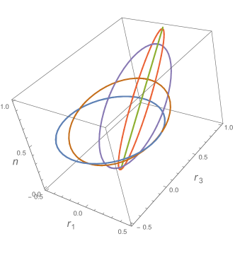
Consider the family $\rho_{AB}(\alpha,\eta):=\eta{|\phi_{\alpha}\rangle\!\langle\phi_{\alpha}|}+(1-\eta)\mathbb{I}/4$, where $|\phi_{\alpha}\rangle:=\cos\alpha|00\rangle+\sin\alpha|11\rangle$ for $0\leq\alpha\leq\frac{\pi}{4}$. The steering ellipses for these states are $\tilde{\rho}_{B}^{\,\alpha,\eta}(\theta)=\left(\begin{array}[]{cc}\eta\cos^{2}(\alpha)\cos^{2}\left(\frac{\theta}{2}\right)-\frac{\eta}{4}+\frac{1}{4}&\frac{1}{2}\eta\cos(\alpha)\sin(\alpha)\sin(\theta)\\ \frac{1}{2}\eta\cos(\alpha)\sin(\alpha)\sin(\theta)&\eta\sin^{2}(\alpha)\sin^{2}\left(\frac{\theta}{2}\right)-\frac{\eta}{4}+\frac{1}{4}\end{array}\right)$ and are plotted in the Bloch representation in Fig. 3.

Refer to caption
Refer to caption

(a)                      (b)

Figure 3: (a) Steering ellipses in the Bloch representation for $\eta=1$, $\alpha=\pi/4$ (blue), $0.65$ (brown), $0.35$ (purple), $0.1$ (red) and 00 (green); (b) $\alpha=0.35$ and $\eta=1$ (blue), $\frac{3}{4}$ (brown), $\frac{1}{2}$ (purple), $\frac{1}{4}$ (red) and $\eta=0.01$ (green). The small yellow circle on the right marks the origin.

One can verify that for $A_{\alpha}=\left(\begin{array}[]{cc}\sin^{2}\alpha&0\\ 0&\cos^{2}\alpha\end{array}\right)$, ${\rm Tr}(A_{\alpha}\tilde{\rho}_{B}^{\,\alpha,\eta}(\theta))=\frac{1}{8}(2-\eta(1-\cos(4\alpha)))$, which is independent of $\theta$. $A_{\alpha}$ is hence normal to the steering ellipse and so the tilt of the ellipse is $\cos(2\alpha)\leq 1$, and approaches $1$ as $\alpha$ approaches 00.

Remark 18.

The tilt is independent of $\eta$ and hence the steering ellipse for any two-qubit pure state has tilt at most 1.

We have $\rho_{B}(\alpha,\eta)=\frac{1}{2}(1+\eta\cos(2\alpha)){|0\rangle\!\langle 0|}+\frac{1}{2}(1-\eta\cos(2\alpha)){|1\rangle\!\langle 1|}$.

The derivative of the steering ellipse with respect to $\theta$ is

$$\frac{\mathrm{d}}{\mathrm{d}\theta}\tilde{\rho}_{B}^{\,\alpha,\eta}(\theta)=\frac{\eta}{2}\left(\begin{array}[]{cc}-\cos^{2}(\alpha)\sin\left(\theta\right)&\cos(\alpha)\sin(\alpha)\cos(\theta)\\ \cos(\alpha)\sin(\alpha)\cos(\theta)&\sin^{2}(\alpha)\sin\left(\theta\right)\end{array}\right)\,.$$ (64)

For $\alpha=\frac{\pi}{4}$ the case is as before. To investigate other values of $\alpha$, we note that, by Remark 3, if $\rho_{AB}(\alpha,\eta)$ has a LHS model, then so does $\rho_{AB}(\alpha,\eta^{\prime})$ for $\eta^{\prime}<\eta$. Thus, for each $\alpha$ there is a critical value $\bar{\eta}(\alpha)$ such that $\rho_{AB}(\alpha,\eta)$ is RP-steerable for $\eta>\bar{\eta}(\alpha)$ and is RP-unsteerable for $\eta\leq\bar{\eta}(\alpha)$. We search for this critical value numerically.

Since $Y$ has real entries, is positive and multiplying by a constant doesn’t affect whether (45) holds, we can take $Y$ to have ${\rm Tr}(Y)=1$ and parameterize it in terms of two parameters $r_{1}$ and $r_{3}$ using a plane of the Bloch sphere via $Y=\frac{1}{2}(\mathbb{I}+r_{1}\sigma_{1}+r_{3}\sigma_{3})$. To do the search we use the following subroutines:

  1. 1.

    For fixed $\alpha$ and $\eta$ this searches over $r_{1},r_{3}$ to find the largest value of the minimum eigenvalue of the expression on the left of (45). This uses gradient ascent with decreasing step-size, terminating when no improvement can be found for some minimal step-size, or when $r_{1},r_{3}$ are found such that the minimum eigenvalue is positive (i.e., (45) is satisfied). The output is either the largest value found or the first positive value found.

  2. 2.

    This is analogous to Subroutine 1, except it searches for the smallest value of the maximum eigenvalue of the expression on the left of (45), terminating either when a negative value is obtained or when no improvement can be found for some minimal step-size.

  3. 3.

    For fixed $\alpha$, this uses Binary Search to find the largest $\eta$ for which Subroutine 1 returns a positive value, for some number of search steps.

  4. 4.

    For fixed $\alpha$, this uses Binary Search to find the smallest $\eta$ for which Subroutine 2 returns a negative value, for some number of search steps.

Subroutine 3 hence gives a certified lower bound on $\bar{\eta}(\alpha)$ and Subroutine 4 a certified upper bound. By varying the step-sizes and number of steps, in principle, we can make the gap between these as small as we like (in practice, the limits of machine precision provide a cut-off).

Note that if Subroutine 1 has a negative output, we cannot strictly rule out that there exists a $Y$ such that condition (45) holds: in principle a smaller step-size might reveal a suitable $Y$. This is why we use Subroutine 2 in parallel.

The result is given in Figure 1 (although the plot only shows $\eta>0.6$, the region extends to $\eta=0$).

VI.3 RP-steerability of depolarizing channel states

Consider a source that generates an entangled state that is sent to two parties via two depolarizing channels with parameters $\eta_{A}$ and $\eta_{B}$, i.e., these channels take

$$\mathcal{S}(\mathbb{C}^{2}\otimes\mathbb{C}^{2})\to\mathcal{S}(\mathbb{C}^{2}\otimes\mathbb{C}^{2}):\rho_{AB}\mapsto\hat{\rho}_{AB}:=(\mathcal{E}_{\eta_{A}}\otimes\mathcal{E}_{\eta_{B}})(\rho_{AB})\,,$$

where $\mathcal{E}_{\eta}:\mathcal{S}(\mathbb{C}^{2})\to\mathcal{S}(\mathbb{C}^{2})$ is given by $\mathcal{E}_{\eta}(\rho)=\eta\rho+(1-\eta)\mathbb{I}/2$.

For $\rho_{AB}={|\Phi_{+}\rangle\!\langle\Phi_{+}|}$, this channel leads to Werner states (with parameter $\eta_{A}\eta_{B}$ instead of $\eta$). The states are hence RP-unsteerable iff $\eta_{A}\eta_{B}\leq\frac{2}{\pi}\approx 0.637$.

More generally, for $\rho_{AB}={|\phi_{\alpha}\rangle\!\langle\phi_{\alpha}|}$, we call the state after the channel $\hat{\rho}_{AB}(\alpha,\eta_{A},\eta_{B})$ and note that

$$\hat{\rho}_{B}=\frac{1}{2}\left((1+\eta_{B}\cos(2\alpha)){|0\rangle\!\langle 0|}+(1-\eta_{B}\cos(2\alpha)){|1\rangle\!\langle 1|}\right)$$

is independent of $\eta_{A}$. The steering ellipse for such a state is

$$\tilde{\rho}_{B}^{\,\alpha,\eta_{A},\eta_{B}}(\theta)=\frac{1}{4}\left(\begin{array}[]{cc}1+\eta_{A}\cos(2\alpha)\cos(\theta)+\eta_{B}(\eta_{A}\cos(\theta)+\cos(2\alpha))&\eta_{A}\eta_{B}\sin(2\alpha)\sin(\theta)\\ \eta_{A}\eta_{B}\sin(2\alpha)\sin(\theta)&1+\eta_{A}\cos(2\alpha)\cos(\theta)-\eta_{B}(\eta_{A}\cos(\theta)+\cos(2\alpha))\end{array}\right)$$

For $A_{\alpha,\eta_{A},\eta_{B}}=\left(\begin{array}[]{cc}\frac{\eta_{B}-\cos(2\alpha)}{2\eta_{B}}&0\\ 0&\frac{\eta_{B}+\cos(2\alpha)}{2\eta_{B}}\end{array}\right)$, we have ${\rm Tr}(A_{\alpha,\eta_{A},\eta_{B}}\tilde{\rho}_{B}^{\,\alpha,\eta_{A},\eta_{B}}(\theta))=\frac{1}{2}\sin^{2}(2\alpha)$, which is independent of $\theta$. Hence $A_{\alpha,\eta_{A},\eta_{B}}$ is the normal to the steering ellipse, and the ellipse has tilt $\frac{\cos(2\alpha)}{\eta_{B}}$. This is less than 1 for $\eta_{B}>\cos(2\alpha)$, so we can use Theorem 14 and Corollary 15 provided this holds.

The derivative of the steering ellipse is

$$\frac{\mathrm{d}}{\mathrm{d}\theta}\tilde{\rho}_{B}^{\,\alpha,\eta_{A},\eta_{B}}(\theta)=\frac{\eta_{A}}{4}\left(\begin{array}[]{cc}-(\eta_{B}+\cos(2\alpha))\sin(\theta)&\eta_{B}\sin(2\alpha)\cos(\theta)\\ \eta_{B}\sin(2\alpha)\cos(\theta)&(\eta_{B}-\cos(2\alpha))\sin(\theta)\end{array}\right)\,.$$ (65)

Since this is proportional to $\eta_{A}$, the amount of noise on Alice’s side (the untrusted side), the case of noise only on Bob’s side is representative of the general case.

We first make two observations for special cases, before proceeding with the general case:

  1. 1.

    If there is no noise on Bob’s side (i.e., the trusted side), i.e., if $\eta_{B}=1$, then $\frac{\mathrm{d}}{\mathrm{d}\theta}\tilde{\rho}_{B}^{\,\alpha,\eta_{A},1}(\theta)$ is identical to that in (64), and the tilt of the steering ellipse of $\rho_{AB}(\alpha,\eta_{A},1)$ is $\cos(2\alpha)\leq 1$, so we obtain the same result.

  2. 2.

    If the state is maximally entangled, i.e., $\alpha=\frac{\pi}{4}$, then the situation is exactly the same as for a Werner state with $\eta=\eta_{A}\eta_{B}$. In other words, $\eta_{A}\eta_{B}\leq\frac{2}{\pi}$ is a necessary and sufficient condition for RP-unsteerability of a state of the form $\rho_{AB}(\pi/4,\eta_{A},\eta_{B})$.

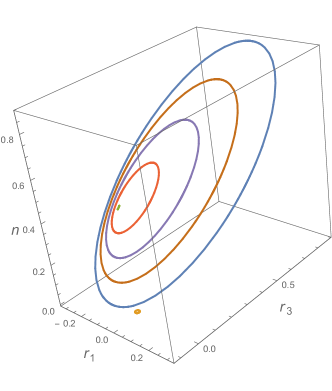
We study the general case numerically, using similar techniques to before. The results are shown in Figure 4.

Refer to caption
Figure 4: Plot of the regions where a LHS model exists for all real projective measurements for $\eta_{A}=1$ (blue), $\eta_{A}=0.9$ (orange) and $\eta_{A}=0.8$ (green), $\eta_{A}=0.7$ (red) (although not shown, all regions extend downwards to $\eta_{B}=0$), together with the purple curve $\eta_{B}=\cos(2\alpha)$ which we need to be above to use Theorem 14 and Corollary 15. In the case $\eta_{A}=\frac{2}{\pi}$ (not shown), the state is RP-unsteerable for all $\eta_{B}$ and $\alpha$. For $\eta_{A}=0.9$, $0.8$ and $0.7$ we have a complete classification: above each of the corresponding regions, the state is RP-steerable. In the case $\eta_{A}=1$, the classification is incomplete for $\alpha\lessapprox 0.37$. Here, if $\eta_{B}\leq\cos(2\alpha)$ we are unable to decide whether or not the states are RP-steerable (while for $\eta_{B}>\cos(2\alpha)$ we know the states are RP-steerable).

The left hand side of (45) becomes easier to satisfy for lower $\eta_{A}$ and so the region of RP-unsteerability increases as $\eta_{A}$ is lowered. In other words, if $\hat{\rho}_{AB}(\alpha,\eta_{A},\eta_{B})$ is RP-unsteerable, then so is $\hat{\rho}_{AB}(\alpha,\eta^{\prime}_{A},\eta_{B})$ for $\eta^{\prime}_{A}\leq\eta_{A}$. At $\eta_{A}=\frac{2}{\pi}$ the state is RP-unsteerable for all $\eta_{B}$ and $\alpha$.

Note that the regions shown in the above plot extend below the purple curve, although the condition on the tilt of the steering ellipse ceases to be satisfied there. To extend to this region we use the fact that more noise (lower $\eta_{B}$) makes a LHS model easier to construct. This is stated in the following lemma.

Lemma 19.

If $\hat{\rho}_{AB}(\alpha,\eta_{A},\eta_{B})$ has a LHS model (for any set of measurements), then so does $\hat{\rho}_{AB}(\alpha,\eta_{A},\eta_{B}^{\prime})$ for all $\eta_{B}^{\prime}<\eta_{B}$.

Proof.

This follows from Remark 3 and the fact that $\hat{\rho}_{AB}(\alpha,\eta_{A},\eta_{B}^{\prime})$ is equal to $\frac{\eta_{B}^{\prime}}{\eta_{B}}\hat{\rho}_{AB}(\alpha,\eta_{A},\eta_{B})+\frac{\eta_{B}-\eta_{B}^{\prime}}{\eta_{B}}\hat{\rho}_{A}(\alpha,\eta_{A},\eta_{B})\otimes\mathbb{I}/2,$ i.e., is a convex combination of $\hat{\rho}_{AB}(\alpha,\eta_{A},\eta_{B})$ and $\hat{\rho}_{A}(\alpha,\eta_{A},\eta_{B})\otimes\mathbb{I}/2$, both of which have LHS models. ∎

Hence, although we cannot use Theorem 14 throughout the $\alpha$-$\eta_{B}$ plane, we can nevertheless establish steerability of all states of the form $\hat{\rho}_{AB}(\alpha,1,\eta_{B})$ for $\alpha\gtrapprox 0.37$ (for example). Furthermore, the numerics point to the existence of a critical value around $0.92$ such that for values of $\eta_{A}$ below this we can always use our criteria (graphically, the boundary of the region in which a LHS model exists always lies above $\eta_{B}=\cos(2\alpha)$ for $\eta_{A}\lessapprox 0.92$).

Acknowledgements.
We are grateful to Kim Winick for numerous helpful discussions, to Emanuel Knill, Sania Jevtic, Stephen Jordan, and Chau Nguyen for useful feedback on an earlier version of the manuscript, and to Nicholas Brunner, Daniel Cavalcanti and Ivan Supic for pointers to the literature. RC is supported by the EPSRC’s Quantum Communications Hub (grant number EP/M013472/1) and by an EPSRC First Grant (grant number EP/P016588/1). CAM and YS were supported in part by US NSF grants 1500095, 1526928, and 1717523. YS was also supported in part by University of Michigan.

Appendix A Summary of known results for Werner states

Werner states (cf. (2)) are separable if and only if $\eta\leq\frac{1}{3}$ Werner , are steerable if $\eta>\frac{1}{2}$ Wiseman:2007 and are non-local if $\eta>1/K_{G}(3)$ AGT06 , where $K_{G}(3)$ is Grothendieck’s constant of order 3 Grothendieck , which is known to satisfy $1.426<K_{G}(3)<1.464$, so that $0.683<1/K_{G}(3)<0.701$ Brierly ; Hirsch17 . They are local for projective measurements if $\eta\leq 1/K_{G}(3)$ AGT06 and are local for all measurements for $\eta\leq 0.455$ Hirsch17 and also have a LHS model for all measurements for $\eta\leq 5/12$ Barrett02 ; Quintino15 . For $1/3<\eta\leq 5/12$ the states are non-separable and unsteerable. For $\frac{1}{2}<\eta\leq\frac{1}{K_{G}(3)}$ the states are local for projective measurements and steerable. It is unknown whether these states are local for all measurements anywhere in this range, which would show steerability $\kern 6.00006pt\not\kern-6.00006pt\implies$ non-locality, however, this non-implication is known using another family of states Quintino15 .

The above is summarized in Figure 5.

Refer to caption
Figure 5: Summary of known results for Werner states. The approximation taken for $1/K_{G}(3)$ is the mean of the known upper and lower bounds.

Appendix B Additional Proofs

B.1 Proof of Proposition 5

This proof uses similar methods to those in Nguyen:2016 .

The proof will be divided into two cases: (1) the case where $z$ lies on the boundary of $\textnormal{Box}(\mu)$, and (2) the case where $z$ lies in the interior of $\textnormal{Box}(\mu)$.

(1) In the case where $z$ lies on the boundary of $\textnormal{Box}(\mu)$, because $\textnormal{Box}(\mu)$ is convex, there must exist $H\in\mathcal{RA}(\mathbb{C}^{2})$ such that the function $x\mapsto\left<x,H\right>$ on $\textnormal{Box}(\mu)$ is maximized at $z$. We subdivide into three cases depending on $H$.

Case 1a: The element $z$ is on the boundary and $H>0$.

The operator

$\displaystyle\rho$ $\displaystyle=$ $\displaystyle\int_{x\in\mathbb{RP}^{1}}x\ \mathrm{d}\mu$ (66)

is greater than or equal to $z$, so $\left<\rho-z,H\right>\geq 0$. But this quantity cannot exceed 00 by assumption, so $\left<\rho-z,H\right>=0$, which yields $\rho=z$. Since the constant function $\mathbb{RP}^{1}\to\{1\}$ satisfies the definition of a two-step function, we are done.

Case 1b: The element $z$ is on the boundary and $H\ngeq 0$.

In this case, there are unique distinct elements $y,w\in\mathbb{RP}^{1}$ such that $\left<y,H\right>=\left<w,H\right>=0$, $\left<x,H\right>>0$ for all $x\in(y,w)$, and $\left<x,H\right><0$ for all $x\in(w,y)$. Choose a function $f\colon\mathbb{RP}^{1}\to[0,1]$ such that

$\displaystyle z=\int_{x\in\mathbb{RP}^{1}}xf(x)\ \mathrm{d}\mu$ (67)

(such a function must exist because $z\in\textnormal{Box}(\mu)$). Let $g$ be the two step-function

$\displaystyle g(x)$ $\displaystyle=$ $\displaystyle\left\{\begin{array}[]{ccl}1&\textnormal{ if }&x\in(y,w)\\ 0&\textnormal{ if }&x\in(w,y)\\ f(y)&\textnormal{ if }&x=y\\ f(w)&\textnormal{ if }&x=w.\end{array}\right.$ (72)

and let

$\displaystyle r$ $\displaystyle=$ $\displaystyle\int_{x\in\mathbb{RP}^{1}}xg(x)\ \mathrm{d}\mu\,.$ (73)

Since $r\in\textnormal{Box}(\mu)$, $\left<r,H\right>\leq\left<z,H\right>$. Hence we have

$\displaystyle 0\geq\left<r-z,H\right>$ $\displaystyle=$ $\displaystyle\left<\int_{x\in(y,w)}(1-f(x))x\ \mathrm{d}\mu,H\right>-\left<\int_{x\in(w,y)}f(x)x\ \mathrm{d}\mu,H\right>\geq 0\,,$ (74)

where the final inequality follows because any operator $x\in(y,w)$ has positive inner product with $H$ and any operator $x\in(w,y)$ has negative inner product with $H$. It follows that $z=r$, which completes this case.

Case 1c: The element $z$ is on the boundary and $H$ is positive semidefinite and rank-one.

Let $y\in\mathbb{RP}^{1}$ be the unique element such that $\left<H,y\right>=0$. Let

$\displaystyle g(x)$ $\displaystyle=$ $\displaystyle\left\{\begin{array}[]{ccl}1&\textnormal{ if }&x\neq y\\ f(y)&\textnormal{ if }&x=y\,,\end{array}\right.$ (77)

where $f\colon\mathbb{RP}^{1}\to[0,1]$ is a function such that (67) holds. By similar reasoning as in Case 1b, this function also computes $z$.

Case 2: The element $z$ is in the interior of $\textnormal{Box}(\mu)$.

Let

$\displaystyle c$ $\displaystyle=$ $\displaystyle\int_{x\in\mathbb{RP}^{1}}(1/2)x\ \mathrm{d}\mu.$ (78)

Since $z$ is interior it can be written as $z=tc+(1-t)b$, where $t\in[0,1]$ and $b$ is an element on the boundary of $\textnormal{Box}(\mu)$. Let $g$ be a two-step function which computes $b$, which must exist from the first part of the proof. Then, the function $t/2+(1-t)g$ computes $z$. ∎

B.2 Proof of Lemma 7

We will construct an explicit curve which is the boundary of (21). Let $S=\{s_{1},\ldots,s_{n}\}$ be the support of $\mu$, where the points ${|0\rangle\!\langle 0|},s_{1},\ldots,s_{n}$ are in clockwise order, and define $\tilde{\rho}_{m}:=\sum_{i=1}^{m}\mu(s_{i})s_{i}$.

For any $t\in[0,\left<H,\rho\right>]$, define a two-step function $h_{t}\colon\mathbb{RP}^{1}\to[0,1]$ as follows: if

$\displaystyle t\in\left[\left<\rho_{m},H\right>,\left<\rho_{m+1},H\right>\right),$ (79)

then

$\displaystyle h_{t}(x)$ $\displaystyle=$ $\displaystyle 1\quad\text{for }x\in\left[{|0\rangle\!\langle 0|},s_{m+1}\right)$ (80)
$\displaystyle h_{t}(s_{m+1})$ $\displaystyle=$ $\displaystyle\left(\frac{t-\left<\rho_{m},H\right>}{\mu(s_{m+1})\left<s_{m+1},H\right>}\right),$ (81)

and $h_{t}$ is zero elsewhere. Note that, by construction,

$\displaystyle\int_{x\in\mathbb{RP}^{1}}h_{t}(x)\left<x,H\right>\ \mathrm{d}\mu$ $\displaystyle=$ $\displaystyle t.$ (82)

Also define a zero-bias two-step function $\overline{h}_{t}\colon\mathbb{RP}^{1}\to[0,1]$ by

$\displaystyle\overline{h}_{t}$ $\displaystyle=$ $\displaystyle\left\{\begin{array}[]{ll}h_{\left(t+\left<\rho,H\right>/2\right)}-h_{t}&\hskip 21.68121pt\textnormal{ if }t<\left<\rho,H\right>/2\\ \\ 1-h_{t}+h_{\left(t-\left<\rho,H\right>/2\right)}&\hskip 21.68121pt\textnormal{ otherwise,}\\ \end{array}\right.$ (86)

so that for any $t$,

$\displaystyle\int_{x\in\mathbb{RP}^{1}}\overline{h}_{t}(x)\left<x,H\right>\ \mathrm{d}\mu$ $\displaystyle=$ $\displaystyle\left<\rho,H\right>/2.$ (87)

Let

$\displaystyle G(t)$ $\displaystyle=$ $\displaystyle\int_{x\in\mathbb{RP}^{1}}\overline{h}_{t}(x)x\ \mathrm{d}\mu.$ (88)

The points in the image of $G(t)$ are in the region (21) by construction, and since they are obtained from zero-bias two-level functions, they lie on the boundary of $\textnormal{Box}(\mu)$ (see Proposition 5). The image of $G$ is the boundary of (21).

Note that for any fixed $i$, the function $t\mapsto\overline{h}_{t}(s_{i})$ is bitonic (in the sense that it only increases once and decreases once, modulo $\left<\rho,H\right>$) and thus

$\displaystyle\int_{0}^{\left<\rho,H\right>}\left|\frac{\mathrm{d}}{\mathrm{d}t}\left(\overline{h}_{t}(s_{i})\right)\right|\mathrm{d}t\leq 2.$ (89)

Therefore, the length of the curve $G$ satisfies

$\displaystyle\int_{0}^{\left<\rho,H\right>}\left\|\frac{\mathrm{d}}{\mathrm{d}t}G(t)\right\|_{1}\mathrm{d}t$ $\displaystyle=$ $\displaystyle\int_{0}^{\left<\rho,H\right>}\left\|\frac{\mathrm{d}}{\mathrm{d}t}\int_{x\in\mathbb{RP}^{1}}\overline{h}_{t}(x)x\mathrm{d}\mu\right\|_{1}\mathrm{d}t$ (90)
$\displaystyle=$ $\displaystyle\int_{0}^{\left<\rho,H\right>}\left\|\frac{\mathrm{d}}{\mathrm{d}t}\sum_{i=1}^{n}\overline{h}_{t}(s_{i})s_{i}\mu(s_{i})\right\|_{1}\mathrm{d}t$ (91)
$\displaystyle\leq$ $\displaystyle\int_{0}^{\left<\rho,H\right>}\sum_{i=1}^{n}\left|\frac{\mathrm{d}}{\mathrm{d}t}\left(\overline{h}_{t}(s_{i})\right)\right|\mu(s_{i})\ \mathrm{d}t$ (92)
$\displaystyle\leq$ $\displaystyle\sum_{i=1}^{n}2\mu(s_{i})=2\,,$ (93)

as desired.∎

B.3 Tilt of the derivative of the steering ellipse

Lemma 20.

Suppose $\lambda,\mu\in\mathcal{R}\mathcal{A}(\mathbb{C}^{2})$ with ${\rm Tr}(\lambda\mu)=0$ and ${\rm Tilt}(\mu)<1$. Then ${\rm Tilt}(\lambda)>1$.

Proof.

Suppose $\lambda=\frac{1}{2}(n\mathbb{I}+r_{1}\sigma_{1}+r_{3}\sigma_{3})$ and $\mu=\frac{1}{2}(m\mathbb{I}+s_{1}\sigma_{1}+s_{3}\sigma_{3})$ and write $(r_{1},r_{3})=r{\bf e}_{r}$ and $(s_{1},s_{3})=s{\bf e}_{s}$, where ${\bf e}_{r},{\bf e}_{s}$ are unit vectors and $r,s\geq 0$.

The condition ${\rm Tr}(\lambda\mu)=0$ can be written $-{\bf r}.{\bf s}=nm$. ${\rm Tilt}(\mu)<1$ is equivalent to $s^{2}<m^{2}$. It follows that $({\bf r}.{\bf s})^{2}=n^{2}m^{2}>n^{2}s^{2}$. This rearranges to $({\bf r}.{\bf e_{s}})^{2}>n^{2}$, from which it follows that $r^{2}>n^{2}$, i.e., ${\rm Tilt}(\lambda)>1$. ∎

Corollary 21.

Let $\rho_{AB}\in\mathcal{R}\mathcal{D}(\mathbb{C}^{2}\otimes\mathbb{C}^{2})$ be a two-qubit state whose steering ellipse $\{\tilde{\rho}_{B}(\theta)\}$ has tilt smaller than $1$. Then ${\rm Tilt}(\frac{\mathrm{d}}{\mathrm{d}\theta}\tilde{\rho}_{B}(\theta))>1$ for all $\theta$.

B.4 A topological lemma

Lemma 22.

Let $D=\{z\in\mathbb{C}\mid\left|z\right|\leq 1\}$ and let $S^{1}=\{z\in\mathbb{C}\mid\left|z\right|=1\}$. Let $F\colon D\to D$ be a continuous function such that for any $z\in S^{1}$, $F(z)=-z$. Then, $F$ is onto.

Proof.

Suppose, for the sake of contradiction, that $y\in D\smallsetminus F(D)$. Let $G\colon D\to S^{1}$ be the (unique) function defined by the condition that for any $z\in D$, $F(z)$ lies on the line segment from $y$ to $G(z)$. Note that the function $G$ also satisfies $G(z)=-z$ for $z\in S^{1}$. The family of functions $\left\{H_{\alpha}\colon S^{1}\to S^{1}\mid\alpha\in[0,1]\right\}$ given by $H_{\alpha}(z)=G(\alpha z)$ is a continuous deformation between the negation map on $S^{1}$ and the constant map which takes $S^{1}$ to $G(0)$. This is impossible, since these maps represent different elements of the fundamental group of $S^{1}$. Thus, by contradiction, the original map $F$ must be onto. ∎

B.5 Proof of Proposition 11

By Proposition 10, we have

$\displaystyle\left|X\right|_{Y}$ $\displaystyle=$ $\displaystyle Y^{-1}\left|YXY\right|Y^{-1}$ (94)
$\displaystyle=$ $\displaystyle\frac{Y^{-1}(YXY)(YXY)Y^{-1}-Y^{-1}(YXY)(\hat{Y}\hat{X}\hat{Y})Y^{-1}}{\left\|YXY\right\|_{1}}$ (95)
$\displaystyle=$ $\displaystyle\frac{XY^{2}X-X\det(Y)\hat{X}\hat{Y}Y^{-1}}{\left\|YXY\right\|_{1}}$ (96)
$\displaystyle=$ $\displaystyle\frac{XY^{2}X-X\hat{X}\hat{Y}(\det(Y)Y^{-1})}{\left\|YXY\right\|_{1}}$ (97)
$\displaystyle=$ $\displaystyle\frac{XY^{2}X-\det(X)\hat{Y}\hat{Y}}{\left\|YXY\right\|_{1}},$ (98)

which is equal to the desired formula.

References

  • (1) Bell, J. S. On the Einstein-Podolsky-Rosen paradox. In Speakable and unspeakable in quantum mechanics, chap. 2 (Cambridge University Press, 1987).
  • (2) Mayers, D. & Yao, A. Quantum cryptography with imperfect apparatus. In Proceedings 39th Annual Symposium on Foundations of Computer Science (Cat. No.98CB36280), 503–509 (1998).
  • (3) Barrett, J., Hardy, L. & Kent, A. No signalling and quantum key distribution. Physical Review Letters 95, 010503 (2005). URL https://doi.org/10.1103/PhysRevLett.95.010503.
  • (4) Wiseman, H. M., Jones, S. J. & Doherty, A. C. Steering, entanglement, nonlocality, and the Einstein-Podolsky-Rosen paradox. Phys. Rev. Lett. 98, 140402 (2007). URL http://link.aps.org/doi/10.1103/PhysRevLett.98.140402.
  • (5) Branciard, C., Cavalcanti, E. G., Walborn, S. P., Scarani, V. & Wiseman, H. M. One-sided device-independent quantum key distribution: Security, feasibility, and the connection with steering. Phys. Rev. A 85, 010301 (2012). URL https://link.aps.org/doi/10.1103/PhysRevA.85.010301.
  • (6) Piani, M. & Watrous, J. Necessary and sufficient quantum information characterization of Einstein-Podolsky-Rosen steering. Phys. Rev. Lett. 114, 060404 (2015). URL https://link.aps.org/doi/10.1103/PhysRevLett.114.060404.
  • (7) Cavalcanti, D., Guerini, L., Rabelo, R. & Skrzypczyk, P. General method for constructing local hidden variable models for entangled quantum states. Phys. Rev. Lett. 117, 190401 (2016). URL https://doi.org/10.1103/PhysRevLett.117.190401.
  • (8) Hirsch, F., Quintino, M. T., Vértesi, T., Pusey, M. F. & Brunner, N. Algorithmic construction of local hidden variable models for entangled quantum states. Phys. Rev. Lett. 117, 190402 (2016). URL https://doi.org/10.1103/PhysRevLett.117.190402.
  • (9) Werner, R. F. Quantum states with Einstein-Podolsky-Rosen correlations admitting a hidden-variable model. Phys. Rev. A 40, 4277–4281 (1989). URL https://doi.org/10.1103/PhysRevA.40.4277.
  • (10) Jevtic, S., Hall, M. J. W., Anderson, M. R., Zwierz, M. & Wiseman, H. M. Einstein–Podolsky–Rosen steering and the steering ellipsoid. J. Opt. Soc. Am. B 32, A40–A49 (2015). URL http://josab.osa.org/abstract.cfm?URI=josab-32-4-A40.
  • (11) Nguyen, H. C. & Vu, T. Nonseparability and steerability of two-qubit states from the geometry of steering outcomes. Phys. Rev. A 94, 012114 (2016). URL http://doi.org/10.1103/PhysRevA.94.012114.
  • (12) Nguyen, H. C. & Vu, T. Necessary and sufficient condition for steerability of two-qubit states by the geometry of steering outcomes. Europhysics Letters 115, 10003 (2016). URL http://stacks.iop.org/0295-5075/115/i=1/a=10003.
  • (13) Jones, S. J., Wiseman, H. M. & Doherty, A. C. Entanglement, Einstein-Podolsky-Rosen correlations, Bell nonlocality, and steering. Phys. Rev. A 76, 052116 (2007). URL https://doi.org/10.1103/PhysRevA.76.052116.
  • (14) Bowles, J., Hirsch, F., Quintino, M. T. & Brunner, N. Sufficient criterion for guaranteeing that a two-qubit state is unsteerable. Phys. Rev. A 93, 022121 (2016). URL https://link.aps.org/doi/10.1103/PhysRevA.93.022121.
  • (15) Jones, S. J. & Wiseman, H. M. Nonlocality of a single photon: Paths to an einstein-podolsky-rosen-steering experiment. Phys. Rev. A 84, 012110 (2011). URL http://doi.org/10.1103/PhysRevA.84.012110.
  • (16) Uola, R., Luoma, K., Moroder, T. & Heinosaari, T. Adaptive strategy for joint measurements. Phys. Rev. A 94, 022109 (2016). URL http://doi.org/10.1103/PhysRevA.94.022109.
  • (17) Jevtic, S., Pusey, M., Jennings, D. & Rudolph, T. Quantum steering ellipsoids. Phys. Rev. Lett. 13, 020402 (2014). URL https://doi.org/10.1103/PhysRevLett.113.020402.
  • (18) Simmons, G. F. Introduction to Topology and Modern Analysis (Krieger Publishing Company, 1983), reprint edn.
  • (19) Quintino, M. T. et al. Inequivalence of entanglement, steering, and Bell nonlocality for general measurements. Phys. Rev. A 92, 032107 (2015). URL http://doi.org/10.1103/PhysRevA.92.032107.
  • (20) Bavaresco, J. et al. Most incompatible measurements for robust steering tests. Phys. Rev. A 96, 022110 (2017). URL http://doi.org/10.1103/PhysRevA.96.022110.
  • (21) Acín, A., Gisin, N. & Toner, B. Grothendieck’s constant and local models for noisy entangled quantum states. Phys. Rev. A 73, 062105 (2006). URL http://doi.org/10.1103/PhysRevA.73.062105.
  • (22) Grothendieck, A. Résumé de la théorie métrique des produits tensoriels topologiques. Bol. Soc. Mat. São Paulo 8, 1–79 (1953).
  • (23) Brierley, S., Navascués, M. & Vértesi, T. Convex separation from convex optimization for large-scale problems. e-print arXiv:1609.05011 (2016).
  • (24) Hirsch, F., Quintino, M. T., Vértesi, T., Navascués, M. & Brunner, N. Better local hidden variable models for two-qubit Werner states and an upper bound on the Grothendieck constant $K_{G}(3)$. Quantum 1, 3 (2017). URL https://doi.org/10.22331/q-2017-04-25-3.
  • (25) Barrett, J. Nonsequential positive-operator-valued measurements on entangled mixed states do not always violate a Bell inequality. Phys. Rev. A 65, 042302 (2002). URL http://doi.org/10.1103/PhysRevA.65.042302.