Multilevel preconditioning of Polynomial Chaos Method for quantifying uncertainties in a blood pump

Abstract

Heart failure (HF) is a severe cardiovascular disease, it happens when the heart muscle is so weakened such that it can not provide sufficient blood as body needs. More than 23 million people are suffered by HF worldwide. Despite the modern transplant operation is well established, the lack of heart donations becomes a big restriction on transplantation frequency. With respect to this matter, ventricular assist devices (VADs) can play an important role in supporting patients during waiting period and after the surgery.

Moreover, it has been shown that VADs by means of blood pump have advantages for working under different conditions. While a lot of work has been done on modeling the functionality of the blood pump, but quantifying uncertainties in a numerical model is a challenging task. We consider the Polynomial Chaos (PC) method, which is introduced by Wiener for modeling stochastic process with Gaussian distribution. The Galerkin projection, the intrusive version of the generalized Polynomial Chaos (gPC), has been densely studied and applied for various problems. The intrusive Galerkin approach could represent stochastic process directly at once with Polynomial Chaos series expansions, it would therefore optimize the total computing effort comparing with classical non-intrusive methods. We compared different preconditioning techniques for a steady state simulation of a blood pump configuration in our previous work, the comparison shows that an inexact multilevel preconditioner has a promising performance. In this work, we show an instationary blood flow through a FDA blood pump configuration with Galerkin Projection method, which is implemented in our open source Finite Element library Hiflow3. Three uncertainty sources are considered : inflow boundary condition, rotor angular speed and dynamic viscosity, the numerical results are demonstrated with more than 30 Million degrees of freedom by using supercomputer.

Chen Song, Vincent Heuveline

1 INTRODUCTION

Since last two decades, medical instruments have been playing an important role in the field of health care, they sustain patients’ life by providing advanced clinical solutions or help surgeons to obtain better medical diagnosis. The innovation of medical devices expanded significantly recent years owing to the improvement of mechanical design, numerical modeling, computing hardware, etc. Especially, the blood pump device became one of the most popular assist apparatuses in heart failure treatment [4, 8, 23]. Ventricular assist devices (VADs) can be applied as long-term implant for patients who are not eligible for heart transplantation, or served as a generation of sufficient blood flow for patients during the surgery. However, the verification and validation (V&V) procedure is still demanding due to the lack of knowledge about input parametric data, specially for numerical modeling. Whereas, these uncertainties should not be ignored, because quantifying the impact of these uncertainties can be one of the key points for patient-specific implantation.

In our previous work [26], we investigate the steady state of Navier-Stokes equations for laminar flow in a blood pump geometry. We modeled the rotating impact with the Multiple Reference Frame (MRF) method [7, 20, 10], for quantifying uncertainties, we employed the intrusive Polynomial Chaos Expansion (PCE) method in order to take geometrical uncertainty and specific model parameters into account. We placed also our attention on comparing different solving strategies for the intrusive Polynomial Chaos approach for fluid problem, as being capable of solving efficiently this highly coupled system is very crucial in practice.

In this paper, we will analyze an unsteady blood flow in a blood pump device based on the Variational Multi-Scale method (VMS) for the incompressible Navier-Stokes equations. We concentrate again three different uncertainty sources: inflow boundary condition, dynamic viscosity and angular speed of the rotor. The geometry of the blood pump is referred to the U.S. Food and Drug Administration (FDA) ”critical path” initiative benchmark problem [13], the aim of this project is to utilize advanced computational simulations to predict the biological response. So as to cope with the rotating machinery modelization, we employ a shear layer update approach, which is very similar to The Shear-Slip Mesh Update Method (SSMUM) [2, 3], the main difference is to deploy two layers instead of one in order to facilitate the update process once a regeneration of the mesh is needed. By this setting, the local linear algebra structure remains the same, hence, only few values demand update. We employ the Variational Multi-Scale method [11, 22], which inherits the consideration of two separated scales from the large eddy simulation (LES) model and the concept of stabilized finite element method [28], it provides the feasibility of modeling the blood flow within the high rotation speed instrument.

We here apply the stochastic finite element method (SFEM) [14], this conveys that the spatial domain is discretized by the finite element method (FEM), and the stochastic space is expressed by Polynomial Chaos Expansion(PCE) [29]. One important advantage of utilizing PCE is when the model output is smooth regarding to the input, a spectral convergence of PCE is achieved [9]. PCE exhibits the stochastic solution via the orthogonal multivariate polynomials, and the input random variables are represented in predefined polynomials regarding to their probability distribution. The stochastic Galerkin projection [14, 21] is a powerful tool, which provides the possibility to obtain the coefficients of the PCE system at once. However, efficient solving strategies are needed for such complex structure. From our previous contribution [26], we compared three different preconditioning techniques for a stationary flow in a simplified blood pump geometry, the inexact Multilevel method outperformed the Mean based preconditioner and the exact Multilevel method. We focus therefore in this paper on the inexact Multilevel method, and apply it to the instationary flow in the pump geometry.

The rest of this paper is organized as follow. In Section 2, we introduce the mathematical modeling for high Reynolds number flow in a rotating machinery, illustrate our moving mesh technique and the modelization of stochastic system. Section 3 presents our Multilevel preconditioner algorithm. The numerical results are showed in Section 4. We conclude our contribution and provide an outlook for further development in Section 5.

2 MATHEMATICAL MODELING

We consider the unsteady state of the incompressible Navier-Stokes equations in a rotating machinery, it yields:

$$\frac{\partial\bm{u}}{\partial t}+((\bm{u}-\bm{u}^{r})\cdot\nabla)\bm{u}-\frac{\mu}{\rho}\Delta\bm{u}+\frac{1}{\rho}\nabla p =0\;, \text{in}\>\Omega\;,$$ (1a)

$$\nabla\cdot\bm{u} =0\;, \text{in}\>\Omega\;,$$ (1b)

$$\bm{u}^{r} =\bm{d}\times\bm{\omega}\;, \text{in}\>\Omega_{rot}\;,$$ (1c)

$$\bm{u}^{r} =0\;, \text{in}\>\Omega_{stat}\;,$$ (1d)

$$\bm{u} =\bm{g}\;, \text{on}\>\Gamma_{in}\;,$$ (1e)

$$(\frac{\mu}{\rho}\nabla\bm{u}-p\mathds{1}) =0\;, \text{on}\>\Gamma_{out}\;,$$ (1f)

$$\bm{u}^{r} =\bm{d}\times\bm{\omega}\;, \text{on}\>\Gamma_{rotor}\;,$$ (1g)

$$\bm{u} =0\;, \text{on}\>\partial\Omega\backslash(\Gamma_{in}\cup\Gamma_{out}\cup\Gamma_{rotor})\;.$$ (1h)

Where, $\bm{u}$ is the velocity, and $p$ is the pressure. The flow is described on $\Omega\subset\mathbb{R}^{3}$, $\Omega=\Omega_{rot}\cup\Omega_{stat}$, $\Omega_{stat}\cap\Omega_{rot}=\emptyset$. $\Omega_{stat}$ and $\Omega_{rot}$ denote static and rotating domain respectively [3]. $\bm{u}^{r}$ is the rotation speed, which pre-describes the motion of a moving mesh, it is defined by the angular speed $\bm{\omega}$ and the distance to the rotating axis $\bm{d}$. $\mu$ is the dynamic viscosity and $\rho$ is the density. We ignore here the external body force $\bm{f}$ in N-S equations.

We prescribe a ”do-nothing” condition on the outflow boundary $\Gamma_{out}$, two different Dirichlet boundary conditions are applied on the inflow boundary $\Gamma_{in}$ and the rotor’s surface $\Gamma_{rotor}$ separately. The rest of boundary is covered by ”no-slip” condition (Figure 1). The inflow boundary condition is modeled with a Poiseuille profile:

$$\bm{g}=\begin{bmatrix}0\\ 0\\ -U_{max}(1-l^{2}/L^{2})\end{bmatrix}\;,$$ (2)

$L$ is the radius of the circular inflow boundary, $l$ is the distance from a point on $\Gamma_{in}$ to the center point. $U_{max}$ is the maximum inflow speed, and $U_{max}>0$, as the inflow direction is in $-\bm{e}_{3}=[0,0,-1]^{T}$.

The angular speed is defined as:

$$\bm{\omega}=\begin{bmatrix}0\\ 0\\ \omega\end{bmatrix}\;,$$ (3)

the direction of the axis of rotation for the rotor is showed in Figure 1.

Figure 1: Illustration of the boundaries and the axis of rotation on the blood pump geometry.

2.1 Shear layer update approach

With the purpose of modeling a rotating machinery, we propose here a shear layer update approach, which is inherited from SSMUM [2, 3], we employ though two layers instead of one to achieve the efficiency of the update process once a regeneration of mesh is required. In general, for the mesh patching technique [27], the computational domain is divided by two, static and rotating domain ($\Omega_{stat}$ and $\Omega_{rot}$). The static domain stays unchanged, the rotating domain evolves corresponding the speed of blade.

(a)

(b)

(c)

(d)

Figure 2: Illustration of mesh motion during shear process and reconnecting process.

Figure 2 demonstrates the main procedure of moving mesh for rotating machinery modeling, static and rotating domain own one layer separately and each cell on those two layers has the same shape. The border between these two domains is therefore the interface between the two identical layers as well. At the beginning, the initial position of the mesh looks like in step a, when the rotating part moves in relation to the rotor, we first shear one of these layers in order to obtain more freedom of movement, as we are limited by the mesh size most of the time. The connectivity of mesh cell remains unchanged during the shear process (step b), only spatial location needs to be modified, the adaptation is then uncomplicated. When the shearing attends the same length as the cell (step c). Afterwards, the vertices on the common interface detach, and reconnect to the subsequent points (step d).

If we could ensure that the local mesh only contains either a part of static mesh or rotating mesh (it can be accomplished easily by using group of communicator or similar concept of parallel communication), thus, we would benefit from this setting, as the structure of the local vector does not alter [1]. Therefore, only values on the ghost cells in the local vector need to be updated. For that reason, projecting solution into a new linear algebra structure is avoided, the update process after reconnecting vertices can be accelerated.

2.2 Variational Multiscale method (VMS)

The Reynolds number for a rotating machinery is defined like:

$$Re:=\frac{\omega D^{2}\rho}{\mu}\;,$$ (4)

due to the high rotation speed $\omega$ of our instrument (2500 RPM ), the Reynolds number is approximately $21000$ in our blood pump, an additional high Reynolds number flow modeling is required, we choose in this work the Variational Multiscale method (VMS) for this purpose. This technique considers a separation of complete solution scale into two different groups: resolvable scale and unresolvable scale. In general, VMS can be considered as a kind of stabilized finite element technique [28], whereas, it can also be meanwhile interpreted as large eddy simulation (LES) for turbulence modeling. Without describing the theory, we illustrate only the projection-based finite element variational multiscale method for Navier-Stokes equations. Further insight about this method can be found in [17, 18, 19, 15].

The variational multiscale formulation can only be seen in a weak form:

$$\begin{split}\int_{\Omega}(\frac{\partial\bm{u}}{\partial t}+((\bm{u}-\bm{u}^{r})\cdot\nabla)\bm{u})\cdot\bm{v}\>d\Omega+\int_{\Omega}\frac{\mu}{\rho}\nabla{\bm{u}}:\nabla\bm{v}\>d\Omega-\int_{\Omega}\frac{1}{\rho}p\nabla\cdot\bm{v}\>d\Omega\>d\Omega&\\ +\int_{\Omega}[\frac{\partial\bm{u}}{\partial t}+((\bm{u}-\bm{u}^{r})\cdot\nabla)\bm{u}-\frac{\mu}{\rho}\Delta\bm{u}+\frac{1}{\rho}\nabla p]\tau_{M}((\bm{u}-\bm{u}^{r})\cdot\nabla\bm{v})\>d\Omega&\\ +\int_{\Omega}(\nabla\cdot\bm{u})\cdot\tau_{C}(\nabla\cdot\bm{v})\>d\Omega&=0\;,\end{split}$$ (5a)

$$\begin{split}\int_{\Omega}q\nabla\cdot\bm{u}\>d\Omega&\\ +\int_{\Omega}\tau_{M}\nabla q[\frac{\partial\bm{u}}{\partial t}+(\bm{u}\cdot\nabla)\bm{u}-\frac{\mu}{\rho}\Delta\bm{u}+\frac{1}{\rho}\nabla p]\>d\Omega&=0\;.\end{split}$$ (5b)

$\bm{v}$ and $q$ are the test functions for velocity and pressure. $\tau_{M}$ and $\tau_{C}$ are the elementwise constant stabilization operators, which project the unsolvable solution on the fine scale into the coarse scale based the residual of the governing equations.

2.3 Uncertainty model

We consider three different parametric uncertainties: the inflow boundary condition $\bm{g}$, the angular speed $\bm{\omega}$ and the dynamic viscosity $\mu$. We model each of those uncertain parameters with independent, uniformly distributed random variables $\xi_{i}\sim U(-1,1),i=1,2,3$, it reads:

$$\bm{g} =\bm{g}_{0}+\bm{g}_{1}\xi_{1}\;,$$ (6a)

$$\bm{\omega} =\bm{\omega}_{0}+\bm{\omega}_{2}\xi_{2}\;,$$ (6b)

$$\mu =\mu_{0}+\mu_{3}\xi_{3}\;.$$ (6c)

Where, $\bm{g}_{1}=\sigma_{1}\bm{g}_{0}$, $\bm{\omega}_{2}=\sigma_{2}\bm{\omega}_{0}$ and $\mu_{3}=\sigma_{3}\mu_{0}$. $\sigma_{i}$ are the decay factors respect to the mean value, thus $0<\sigma_{i}<1$. With reference to PCE, we define a multivariate random variable $\bm{\xi}:=(\xi_{1},\xi_{2},\xi_{3})$. Accordingly, $\bm{\xi}$ allows us directly map the outcomes of an abstract probability space $(\Omega,\mathcal{A},\mathbb{P})$ to a subset $T$ of $\mathbb{R}^{3}$. Afterwards, we can express our stochastic solution immediately with the aid of $\bm{\xi}$.

2.4 Stochastic Galerkin projection

The velocity and pressure in Equation 1 are expressed with the Polynomial Chaos Expansion (PCE) method [21] by employing the orthogonal polynomial $\psi$:

$$\bm{u}(\bm{x},\bm{\xi}) =\sum_{i=0}^{\infty}\bm{u}_{i}\psi_{i}(\bm{\xi})\;,$$ (7a)

$$p(\bm{x},\bm{\xi}) =\sum_{i=0}^{\infty}p_{i}\psi_{i}(\bm{\xi})\;.$$ (7b)

$\psi_{i}$ represents the Chaos Polynomials, more specifically in this paper, their are the normalized Legendre Polynomials. $\bm{u}$ and $p$ follow certain general assumptions, such as square-integrable respect to $\bm{\xi}$, more details can be found in [21]. The orthogonality of $\psi_{i}$ with respect to the probability density function of $\bm{\xi}$ can be explicit written as:

$$\int_{[-1,1]^{3}}\psi_{i}(\bm{\xi})\psi_{h}(\bm{\xi})\frac{1}{2^{3}}d\bm{\xi}=\delta_{ij}\;,$$ (8)

$\delta_{ij}$ here is the Kronecker delta function. In order to be able of computing our stochastic solution numerically, we need to truncate Equation 7 up to certain polynomials order $No$, it yields:

$$\bm{u}(\bm{x},\bm{\xi}) \approx\sum_{i=0}^{P}\bm{u}_{i}\psi_{i}(\bm{\xi})\;,$$ (9a)

$$p(\bm{x},\bm{\xi}) \approx\sum_{i=0}^{P}p_{i}\psi_{i}(\bm{\xi})\;.$$ (9b)

$P+1=(M+No)!/(M!No!)$ is the total number of the PC modes, $M$ is the number of uncertain variables, in our case, $M=3$.

Therefore, we could pursuit the generalized Polynomial Chaos Expansion (gPCE) [30] procedure by first inserting Equation 9 into Equation 5, then multiplying an additional polynomial $\psi_{k},k=0,...,P$ on both side of governing equations, and taking $L^{2}$ inner product on $L^{2}(T)$. By considering the orthogonality of the polynomials, the regarding momentum equation and mass conservation can be thus written as:

$$\frac{\partial\bm{u}_{k}}{\partial t}\bm{v}_{k}+\sum_{i=0}^{P}\sum_{j=0}^{P}((\bm{u}_{i}-\bm{u}_{i}^{r})\cdot\nabla)\bm{u}_{j}\bm{v}_{k}c_{ijk}+\sum_{i=0}^{P}\sum_{j=0}^{P}\frac{\mu_{i}}{\rho}\nabla\bm{u}_{i}:\nabla\bm{v}_{j}c_{ijk}+\frac{1}{\rho}p_{i}\nabla\cdot\bm{v}_{k}$$ (10a)

$$+\tau_{M}((\bm{u}_{k}-\bm{u}_{k}^{r})\cdot\nabla\bm{v}_{k})[\frac{\partial\bm{u}_{k}}{\partial t}+\sum_{i=0}^{P}\sum_{j=0}^{P}((\bm{u}_{i}-\bm{u}_{j}^{r})\cdot\nabla)\bm{u}_{j}c_{ijk}$$

$$-\sum_{i=0}^{P}\sum_{j=0}^{P}\frac{\mu_{i}}{\rho}\Delta\bm{u}_{j}c_{ijk}+\frac{1}{\rho}\nabla p_{k}]+(\nabla\cdot\bm{u}_{k})\tau_{C}(\nabla\cdot\bm{v}_{k})\;, \text{in}\>\Omega\;,$$

$$q_{k}\nabla\cdot\bm{u}_{k}$$ (10b)

$$\tau_{M}\nabla q_{k}[\frac{\partial\bm{u}_{k}}{\partial t}+\sum_{i=0}^{P}\sum_{j=0}^{P}((\bm{u}_{i}-\bm{u}_{i}^{r})\cdot\nabla)\bm{u}_{j}c_{ijk}$$

$$-\sum_{i=0}^{P}\sum_{j=0}^{P}\frac{\mu_{i}}{\rho}\Delta\bm{u}_{j}c_{ijk}+\frac{1}{\rho}\nabla p_{k}]\;, \text{in}\>\Omega\;.$$

for $$k=0,...,P c_{ijk}:=<\psi_{i}\psi_{j},\psi_{k}>$$, and .

So fair, we introduce the variational multiscale formulation for the incompressible Navier-Stokes equations in a rotating machinery based on our moving mesh technique, the modeling of input uncertain parameters and the generalized Polynomial Chaos Expansion according to considered problem is also presented. In the following section, we will focus on the numerical methods for solving this specially system.

3 NUMERICAL METHODS

The nonlinear terms in Equation 10 are linearized with Newton method, the general scheme can be written as:

$$\mathbf{J}_{\mathbf{F}}(\bm{x}_{n})(\bm{x}_{n+1}-\bm{x}_{n})=\mathbf{F}(\bm{x}_{n})\;,$$ (11)

$\mathbf{F}$ is the system equation, $\mathbf{J}_{F}$ is the Jacobian matrix of $\mathbf{F}$. $\bm{x}_{n}$ is the solution vector at $n$-th Newton iteration, $\bm{x}_{n}=[\bm{u}_{n},p_{n}]^{T}$. At each Newton iteration, an update ($\bm{x}_{n+1}-\bm{x}_{n}$) of the solution vector will be computed, until it meets to certain convergence criterion.

The spatial part of our problem is therefore discretized by the finite element method with equal order P1/P1 element for velocity and pressure respectively, thanks to VMS, no Taylor-Hood element is necessary. Afterwards, we will obtain a linear system of equations for the variational multiscale formulation for the Navier-Stokes equations in rotating system. The stiffness matrix $A(\bm{x}_{n})\in\mathbb{R}^{(P+1)N,(P+1)N}$ can be expressed as:

$$A(\bm{x_{n}})=\sum_{i=0}^{P}K_{i}\otimes A_{i}(\bm{x_{n}})\;.$$ (12)

Note that, $N$ is the number of degree of freedom for the finite element discretization, $\bm{x}_{n}$ is the linearized point. $A_{i}(\bm{x}_{n})\in\mathbb{R}^{N,N},i=0,...,P$ are the Kronecker factors and $K_{i}\in\mathbb{R}^{P+1,P+1},i=0,...,P$ denote the stochastic Galerkin matrices defined by $(K_{i})_{j,k}=c_{ijk}$, which will play an important role in the multilevel method.

3.1 Multilevel method

Solving a such complex stochastic Galerkin system is very challenging, choosing a good solving strategy is very crucial. The multilevel method has been applied with good convergence behavior [26, 24, 25].

The stochastic Galerkin system possesses a hierarchical structure due to the polynomial construction, thus we make use of this feature. If space $\mathcal{S}_{l}$ is spanned by the Chaos Polynomials:

$$\mathcal{S}_{l}=\text{span}\{\psi_{0},...,\psi_{P_{l}}\}\;,$$ (13)

$l\in\mathbb{N},\;l\leq No$ is certain polynomial degree, $P_{l}=(M+l)!/(M!l!)$. $M$ is again the number of uncertain parameters, in this paper, $M=3$. $P_{l}$ is the total number of PC mode with respect to the polynomial order $l$. The hierarchical space $\mathcal{S}$ can be also expressed as a nested sequence of spaces with the consideration of the total polynomial degree $No$:

$$\mathcal{S}_{0}\subseteq\mathcal{S}_{1}\subseteq\cdots\subseteq\mathcal{S}_{l}\cdots\subseteq\mathcal{S}_{No}\;.$$ (14)

The discretized Newton step of Equation 10 at iteration $n$ based on Equation 13 can be found like:

$$\sum_{i=0}^{P_{No}}K_{i}\otimes A_{i}(\bm{x}_{n})\bm{\tilde{x}}_{n}^{No}=-\bm{b}_{n}^{No}\;.$$ (15)

$\bm{\tilde{x}}_{n}^{No},\bm{b}_{n}^{No}\in\mathbb{R}^{N(P+1)}$, and $\bm{\tilde{x}}_{n}^{No}=\bm{x}_{n+1}^{No}-\bm{x}_{n}^{No}$. We bring into play the principle of multigrid method [5, 6, 16], and consider the polynomial degree $l$ in Equation 14 as the ”grid level”. Hence, the restriction operator $\mathcal{R}_{l-1}$ and the prolongation operator $\mathcal{P}_{l}$ are naturally defined as a $L^{2}$ projection from $\mathcal{S}_{l-1}$ to $\mathcal{S}_{l}$ or vice versa.

One of very crucial procedure for Multilevel method (as well as for Multigrid scheme) is to choose an appropriate smoother, we utilize here the Mean based preconditioner as our smoother [26], we apply $\theta$ times smoothing process to a given initial solution $x_{0}^{l}$:

$$x_{k+1}^{l}:=\mathcal{B}_{l}x_{l}^{l}=x_{k}^{l}+(I_{d}\otimes A_{0})^{-1}\;.$$ (16)

1:  if $l=0$ then

2:     solve $A_{0}x^{0}=b^{0}$

3:  else

4:     $x^{l}=\mathcal{S}^{l}x^{l}$  ($\nu_{1}$ times pre-smoothing)

5:     $r^{l}=b^{l}-\sum_{i=0}^{P_{l}}(K_{i}\otimes A_{i})x^{l}$  (compute residual)

6:     $r^{l-1}=\mathcal{R}_{l-1}r^{l}$  (restriction)

7:     for $i=1$ to $\mu$ do

8:        ML($b^{l-1}$, $x^{l-1}$, $l$)  (V-cycle/W-cycle)

9:     end for

10:     $c^{l}=\mathcal{P}_{l}c^{l-1}$  (prolongation)

11:     $x^{l}=x^{l}+c^{l}$  (update with correction)

12:     $x^{l}=\mathcal{S}^{l}x^{l}$  ($\nu_{2}$ times post-smoothing)

13:  end if

Algorithm 1 PCE Multilevel preconditioner/solver : ML

Figure 3: One cycle of the multilevel method: ML($x^{l},b^{l},l)$ given a vector $x^{l}$ and right hand side $b^{l}$ on level $l$. $\mu=1$ results in a $V$-cycle, $\mu=2$ in a $W$-cycle.

Note that, the subscript $k$ indicates the iteration number within the smoothing procedure, which is not the same for Newton step in Equation 11 and Equation 12. A pseudo algorithm about our stochastic Multilevel solver/preconditioner can be found in Algorithm 1.

4 NUMERICAL RESULTS

We use the Crank-Nicolson time stepping scheme for the instationary Navier-Stokes equations, and the nonlinear system Equation 10 is solved via the inexact Newton scheme, it implies that only an approximated solution is applied for each Newton step. We applied the strategy ”choice 1” of Eisenstat and Walker in [12] with an initial forcing term equals to $0.5$.

Inflow maximal speed ($m/s$)	0.5	Inflow speed variation ($\sigma_{1}$)	10%
Dynamic viscosity ($N\cdot s/m^{2}$)	0.0035	Viscosity variation ($\sigma_{3}$)	10%
Angular speed ($rad/s$)	261.8	Angular speed variation ($\sigma_{2}$)	10%
RPM	2500	Density ($Kg/m^{3}$)	1035

Table 1: Model parameter values.

For each Newton step, we apply an iterative Krylov subspace solver, the flexible generalized minimal residual method (FGMRES), with a Multilevel method preconditioner, which is presented in previous section. For the mean block solver, we use the generalized minimal residual method (GMRES), which is preconditioned with Schur Complement preconditioner. We use an inexact Multilevel method here, it indicates that we compute the inverse of $A_{0}$ only respect to certain lower accuracy criterion. In this case, we solve the linear system with $A_{0}$ (in Equation 16) only up to a relative error $1.0e-1$. In contract, the relative accuracy of the Newton step is set to $1e-9$.

Table 1 indicates the information about input parameters, the Reynolds number, according to Equation 4 is about $210000$. The geometry discretization contains $2,984,259$ unstructured cells, it results thus $2,274,904$ degrees of freedom for the deterministic case. As mentioned in Section 2.3, we consider three different input uncertain parameters:inflow boundary condition, dynamic viscosity and angular speed of the rotor. In this work, we consider the situation that the polynomial degree equals to $3$, which gives us in total $20$ PC modes. Therefore, the total number of degrees of freedom is about $45.5$ Millions.

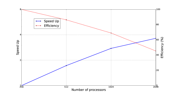
Figure 4: Scalability test with the first $50$ time steps, $3$ uncertainties parameters and polynomial degrees equals to $2$.

Figure 4 shows a scalability test by using the information of the first $50$ time steps. The speed up and the efficiency is defined as $S_{p}:=\frac{T_{1}}{T_{p}},E_{p}:=\frac{S_{p}}{p}$. We find out that the efficiency of our full solving process could still catch around $48\%$ when the number of processor is up to $2048$. We have to mention that we start our test with $256$ processors, because it is the minimal requirement of cores we can use regarding to our problem size, the efficiency of the Multilevel preconditioner itself can perform better if we consider a simpler problem and start the scalability with only one processor.

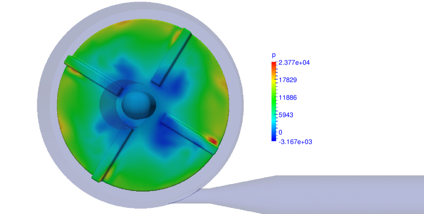
(a) Mean value.

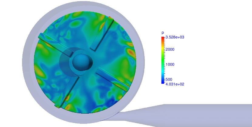
(b) Standard deviation.

Figure 5: The mean value and standard deviation of the pressure at time step = 500.

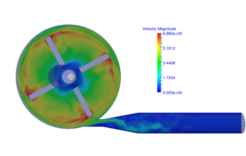
(a) Mean value.

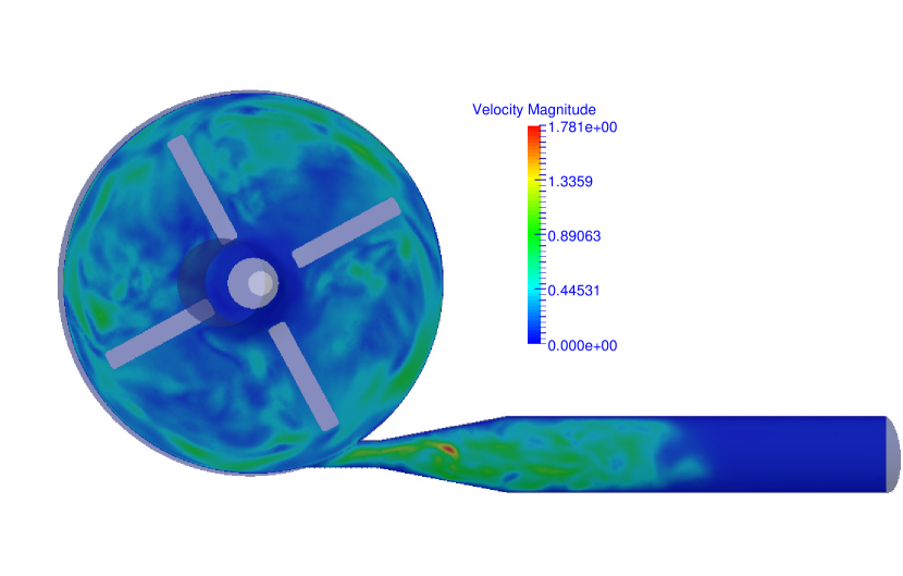
(b) Standard deviation.

Figure 6: The mean value and standard deviation of the velocity at time step = 500.

Figure 5 shows the mean value and standard deviation of pressure distribution on the rotor, the standard deviation follows slightly the magnitude of the mean value, as at the center it is lower and on the hub of the blade is higher. But the uncertainty distribution arises also at certain locations where the pressure is less important. Figure 6 represents the mean value and the standard deviation of the velocity, the standard deviation becomes higher after the flow at the outlet, it might be due to the acceleration after the nozzle structure. Figure 7 represents the value of pressure integration over the rotor. It shows the mean value (red) and mean $\pm$ $3$ standard deviation involving along time.

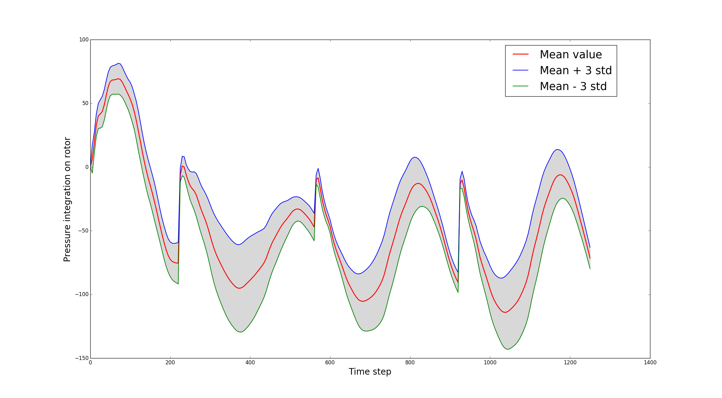
Figure 7: Mean value and mean $\pm$ 3 standard deviation for the pressure integration over the rotor.

5 CONCLUSIONS

This work is a continuation of our last contribution [26], which considered a simplified geometry and an artificial stabilized laminar flow. Within this work, we introduce first with our moving mesh strategy in order to be able of modeling this rotating machine in unsteady state, the evolution speed is therefore coupled into the governing equation. The variational multiscale method offers the viability of modeling the high Reynolds number flow. Hence, the intrusive Polynomial Chaos Expansion method is build upon this modelization for quantifying the impact of different uncertain parameters simultaneously.

Besides mathematical modeling, we place also our interest on the solver/preconditioner technique as solving such a complex system is challenging in practice. We therefore employ the inexact Multilevel preconditioner based on the comparison in our last paper [26] in a large system, we benefit from the low accuracy smoothing process to save computational effort.

Our following work will be focused on developing more analysis about the device’s performance respect to surgical requirements. Further process of post-processing of our numerical simulation data and drawing more insight information about the uncertainties.

6 ACKNOWLEDGMENT

The results of this work is computed on bwForCluster MLS&WISO (production and development). The authors acknowledge support by the state of Baden-Württemberg through bwHPC and the German Research Foundation (DFG) through grant INST 35/1134-1 FUGG. The authors acknowledge support by the Heidelberg Institute for Theoretical Studies, HITS gGmbH.

References

- [1] Hartwig Anzt, Werner Augustin, Martin Baumann, Hendryk Bockelmann, Thomas Gengenbach, Tobias Hahn, Vincent Heuveline, Eva Ketelaer, Dimitar Lukarski, Andrea Otzen, Sebastian Ritterbusch, Björn Rocker, Staffan Ronnas, Michael Schick, Chandramowli Subramanian, Jan-Philipp Weiss, and Florian Wilhelm. Hiflow3 – a flexible and hardware-aware parallel finite element package. Preprint Series of the Engineering Mathematics and Computing Lab, 0(06), 2013.
- [2] M. Behr and T. Tezduyar. The shear-slip mesh update method. Computer Methods in Applied Mechanics and Engineering, 174(3–4):261 – 274, 1999.
- [3] Marek Behr and Dhruv Arora. Shear-slip mesh update method: Implementation and applications. Computer Methods in Biomechanics and Biomedical Engineering, 6(2):113–123, 2003. PMID: 12745425.
- [4] Emma J Birks, Patrick D Tansley, James Hardy, Robert S George, Christopher T Bowles, Margaret Burke, Nicholas R Banner, Asghar Khaghani, and Magdi H Yacoub. Left ventricular assist device and drug therapy for the reversal of heart failure. New England Journal of Medicine, 355(18):1873–1884, 2006.
- [5] Achi Brandt. Multi-level adaptive technique (MLAT) for fast numerical solution to boundary value problems, pages 82–89. Springer Berlin Heidelberg, Berlin, Heidelberg, 1973.
- [6] Achi Brandt. Multi-level adaptive solutions to boundary-value problems. Mathematics of Computation, 31(138):333–390, 1977.
- [7] W. Bujalski, Z. Jaworski, and A.W. Nienow. CFD study of homogenization with dual rushton turbines—comparison with experimental results: Part ii: The multiple reference frame. Chemical Engineering Research and Design, 80(1):97 – 104, 2002. Process and Product Development.
- [8] Daniel Burkhoff, Howard Cohen, Corinna Brunckhorst, and William W. O’Neill. A randomized multicenter clinical study to evaluate the safety and efficacy of the tandemheart percutaneous ventricular assist device versus conventional therapy with intraaortic balloon pumping for treatment of cardiogenic shock. American Heart Journal, 152(3):469.e1 – 469.e8, 2006.
- [9] Thierry Crestaux, Olivier Le Maıˆtre, and Jean-Marc Martinez. Polynomial chaos expansion for sensitivity analysis. Reliability Engineering & System Safety, 94(7):1161 – 1172, 2009. Special Issue on Sensitivity Analysis.
- [10] S.M.A. Cruz, A.J.M. Cardoso, and H.A. Toliyat. Diagnosis of stator, rotor and airgap eccentricity faults in three-phase induction motors based on the multiple reference frames theory. In Industry Applications Conference, 2003. 38th IAS Annual Meeting. Conference Record of the, volume 2, pages 1340–1346 vol.2, Oct 2003.
- [11] T. Dubois, F. Jauberteau, and R. M. Temam. Dynamic Multilevel Methods and Turbulence. John Wiley & Sons, Ltd, 2004.
- [12] Stanley C. Eisenstat and Homer F. Walker. Choosing the forcing terms in an inexact newton method. SIAM Journal on Scientific Computing, 17(1):16–32, 1996.
- [13] U.S. Food and Drug Administration (FDA). Fda’s “critical path” computational fluid dynamics (cfd)/blood damage project, 2013.
- [14] Roger G. Ghanem and Pol D. Spanos. Stochastic Finite Elements: A Spectral Approach. Springer-Verlag New York, Inc., New York, NY, USA, 1991.
- [15] Volker Gravemeier, Stefan Lenz, and Wolfgang A Wall. Variational multiscale methods for incompressible flows. International Journal of Computing Science and Mathematics, 1(2-4):444–466, 2007.
- [16] W. Hackbusch. On the computation of approximate eigenvalues and eigenfunctions of elliptic operators by means of a multi-grid method. SIAM Journal on Numerical Analysis, 16(2):201–215, 1979.
- [17] Thomas JR Hughes, Gonzalo R Feijóo, Luca Mazzei, and Jean-Baptiste Quincy. The variational multiscale method—a paradigm for computational mechanics. Computer methods in applied mechanics and engineering, 166(1-2):3–24, 1998.
- [18] Thomas JR Hughes, Luca Mazzei, and Kenneth E Jansen. Large eddy simulation and the variational multiscale method. Computing and Visualization in Science, 3(1-2):47–59, 2000.
- [19] Volker John and Songul Kaya. A finite element variational multiscale method for the navier–stokes equations. SIAM Journal on Scientific Computing, 26(5):1485–1503, 2005.
- [20] P.C. Krause. Method of multiple reference frames applied to the analysis of symmetrical induction machinery. Power Apparatus and Systems, IEEE Transactions on, PAS-87(1):218–227, Jan 1968.
- [21] O.L. Maitre and O.M. Knio. Spectral Methods for Uncertainty Quantification: With Applications to Computational Fluid Dynamics. Scientific Computation. Springer Netherlands, 2010.
- [22] James M. McDonough and E. C. Hylin. Chaotic small-scale velocity fields as prospective models for unresolved turbulence in an additive decomposition of the navier-stokes equations. International Journal of Fluid Mechanics Research, 26(5-6):539–567, 1999.
- [23] Francis D. Pagani, Leslie W. Miller, Stuart D. Russell, Keith D. Aaronson, Ranjit John, Andrew J. Boyle, John V. Conte, Roberta C. Bogaev, Thomas E. MacGillivray, Yoshifumi Naka, Donna Mancini, H. Todd Massey, Leway Chen, Charles T. Klodell, Juan M. Aranda, Nader Moazami, Gregory A. Ewald, David J. Farrar, and O. Howard Frazier. Extended mechanical circulatory support with a continuous-flow rotary left ventricular assist device. Journal of the American College of Cardiology, 54(4):312 – 321, 2009.
- [24] Eveline Rosseel and Stefan Vandewalle. Iterative solvers for the stochastic finite element method. SIAM Journal on Scientific Computing, 32(1):372–397, 2010.
- [25] M. Schick. A parallel multilevel spectral galerkin solver for linear systems with uncertain parameters. In 2014 22nd Euromicro International Conference on Parallel, Distributed, and Network-Based Processing, pages 352–359, Feb 2014.
- [26] Michael Schick, Chen Song, and Vincent Heuveline. A Polynomial Chaos Method for Uncertainty Quantification in blood pump simulation, pages 93–106. National Technical University of Athens, 2015.
- [27] Joseph L Steger, F Carroll Dougherty, and John A Benek. A chimera grid scheme.[multiple overset body-conforming mesh system for finite difference adaptation to complex aircraft configurations]. In Advances in grid generation; Proceedings of the Applied Mechanics, Bioengineering, and Fluids Engineering Conference, Houston, TX, pages 59–69, 1983.
- [28] Tayfun E Tezduyar. Stabilized finite element formulations for incompressible flow computations. Advances in applied mechanics, 28:1–44, 1991.
- [29] Norbert Wiener. The homogeneous chaos. American Journal of Mathematics, 60(4):897–936, 1938.
- [30] Dongbin Xiu and George E Karniadakis. The wiener-askey polynomial chaos for stochastic differential equations. SIAM Journal on Scientific Computing, 24(2):614–644, 2002.