Total variation regularized non-negative matrix factorization for smooth hyperspectral unmixing

Abstract.

Hyperspectral analysis has gained popularity over recent years as a way to infer what materials are displayed on a picture whose pixels consist of a mixture of spectral signatures. Computing both signatures and mixture coefficients is known as unsupervised unmixing, a set of techniques usually based on non-negative matrix factorization. Unmixing is a difficult non-convex problem, and algorithms may converge to one out of many local minima, which may be far removed from the true global minimum. Computing this true minimum is NP-hard and seems therefore out of reach. Aiming for interesting local minima, we investigate the addition of total variation regularization terms. Advantages of these regularizers are two-fold. Their computation is typically rather light, and they are deemed to preserve sharp edges in pictures. This paper describes an algorithm for regularized hyperspectral unmixing based on the Alternating Direction Method of Multipliers.

Adrien Faivre^∗

Digital Surf, 16 Rue Lavoisier, 25000 Besançon, FRANCE

Email: afaivre@digitalsurf.fr

and

Laboratoire de Mathématiques de Besançon, UMR CNRS 6623,

Université de Bourgogne Franche-Comté,

16 route de Gray, 25030 Besançon cedex, FRANCE

Clément Dombry

Laboratoire de Mathématiques de Besançon, UMR CNRS 6623,

Université de Bourgogne Franche-Comté,

16 route de Gray, 25030 Besançon cedex, FRANCE

Email: clement.dombry@univ-fcomte.fr

1. Hyperspectral unmixing

Spectral sensors can nowadays acquire electromagnetic intensity with a resolution of thousands of wavebands, spread across an increasing number of pixels. Analyzing hyperspectral data is therefore of growing complexity. This article tackles with hyperspectral unmixing, a matrix factorization technique designed to retrieve spectral signatures of pure materials and corresponding proportions from an hyperspectral image, while enhancing smoothness of both spectrums and mixing proportions. Pure spectral signatures and their mixing proportions are usually respectively referred to as endmembers and abundances throughout the hyperspectral analysis literature.

Spectral signatures are by nature positive, and abundances are by definition positive proportions. These facts lead to a formulation of unmixing as the following constrained optimization problem:

(1) $$\min_{W\in\mathbb{R}_{+}^{m\times k},H\in\mathbb{R}_{+}^{k\times n}}\frac{1}{2}\|M-WH\|_{F}^{2},$$

designed to recover $k$ endmembers $W_{1},\cdots,W_{k}$ and their corresponding abundances $H_{1},\cdots,H_{n}$ from $n$ observed spectrums $M_{1},\cdots,M_{n}$. Notations $W_{i},H_{i}$ and $M_{i}$ respectively stand for the $i$-th column of matrices $W,H$ and $M$. The non-negative reals are denoted $\mathbb{R}_{+}$, and $\mathbb{R}_{+}^{m\times n}$ stands for the set of $m\times n$ non-negative matrices. The norm $\|\cdot\|_{F}$ is the standard Frobenius matrix norm.

Problem (1) is known as Non-negative Matrix Factorization (NMF), and is deemed quite difficult. While optimizing with respect to $W$ or $H$ alone is a simple non-negative least squares problem that can be solved in polynomial time, optimizing with both $W$ and $H$ simultaneously turns out to be very hard. Vavasis [14] proved that deciding whether the non-negative rank of a matrix is the same as its rank is NP-complete. Arora et al. [2] showed how under the Exponential Time Hypothesis, there can be no exact algorithm for NMF running in time $(mn)^{o(r)}$. There already exists many algorithms producing approximate solutions to NMF [5]. They range from simple alternating algorithms [10], to more theoretically involved convexifications [9]. In hyperspectral literature, one recurring trend is to try to recover first the endmembers, and only then compute abundances. This is the path followed by VCA [11], SPA [5], SIVM [3], and a few others. Another approach is to add constraints to the NMF problem, aiming for more interesting local minima. The most obvious one we can add is for columns of $H$ to sum to $1$. Abundances are indeed supposed to be proportions. Every column of the abundances matrix must therefore belong to the $k$-simplex. We note:

$$H=\begin{pmatrix}H_{1}&H_{2}&\cdots&H_{n}\end{pmatrix}\in\Delta_{k}^{n}.$$

Hoyer [7] remarked that the matrices resulting from NMF are usually sparse, and emphasized this by adding sparseness constraints on $W$ or $H$. More recently, it was considered natural for abundances to display some sort of spatial regularity across the image. Inspired by Total Variation (TV) regularization techniques, Iordache et al. [8] penalized the $l_{1}$ norm of the abundances gradient. A related idea from Warren and Osher [15] is to consider that endmembers should also display limited total variation. The main topic of the present paper is to combine both spectral and spatial TV regularization to produce a smoothed NMF.

Adding all these constraints and regularizers together yields a goal functional a little more complicated than the one described in Equation (1). The TV regularized NMF problem reads

(2) $$\min_{W\in\mathbb{R}_{+}^{m\times k},H\in\Delta_{k}^{n}}\frac{1}{2}\|M-WH\|_{2}^{2}+\mu\text{TV}(H)+\lambda\text{TV}(W).$$

This problem can fortunately be split into easier sub-problems, through techniques such as the Alternating Direction Method of Multipliers (ADMM). See the seminal paper of Boyd et al. [4] for an in-depth treatment of ADMM techniques.

The ADMM algorithm allows for the optimization of composite problems of the form

(3) $$\min f(x)+g(z)\text{ such that }Ax+Bz=c.$$

To achieve this, first form the augmented Lagrangian

$$L_{\rho}(x,z,y)=f(x)+g(z)+y^{T}(Ax+Bz-c)+\frac{\rho}{2}\|Ax+Bz-c\|_{2}^{2}.$$

Then, using updates

(4) $$\begin{cases}&x_{k+1}=\text{argmin}_{x}L_{\rho}(x,z_{k},y_{k}),\\ &z_{k+1}=\text{argmin}_{z}L_{\rho}(x_{k+1},z,y_{k}),\\ &y_{k+1}=y_{k}+\rho(Ax_{k+1}+Bz_{k+1}-c),\end{cases}$$

one is guaranteed to get a local optimum for problem (3) under relatively mild assumptions. In this paper we will instead use the equivalent shortened version

$$\begin{cases}&x_{k+1}=\text{argmin}_{x}f(x)+\frac{\rho}{2}\|Ax+Bz_{k}-c+u_{k}\|_{2}^{2},\\ &z_{k+1}=\text{argmin}_{z}g(z)+\frac{\rho}{2}\|Ax_{k+1}+Bz-c+u_{k}\|_{2}^{2},\\ &u_{k+1}=u_{k}+(Ax_{k+1}+Bz_{k+1}-c),\end{cases}$$

that follows from Equation (4) by introducing $u_{k}=y/\rho$.

NMF hardly fits the ADMM framework, but Zhang [17] studied the convergence of the following splitting scheme

(5) $$\min_{X_{1},X_{2},Z_{1},Z_{2}}\|M-X_{1}Z_{2}\|_{F}^{2}+\chi_{+}(X_{2})+\chi_{+}(Z_{1})\text{ such that }\begin{cases}X_{1}=Z_{1},\\ X_{2}=Z_{2}.\end{cases}$$

In Equation (5), $\chi_{+}$ denotes the characteristic function of matrices with positive entries, valued $0$ for matrices with no negative entries, and $\infty$ for any other. The sub-problem in $X_{1}$ is a least square problem, and the one in $X_{2}$ can be solved using a projection on the positive orthant. Sub-problems in $Z_{1},Z_{2}$ can be dealt with similarly. These four sub-problems can be solved efficiently. The difference with standard ADMM formulation is that it does not seem possible to properly split Equation (1) as the sum of two functions.

One advantage of the ADMM technique is that adding regularization terms is rather straightforward, enabling us to interleave TV regularization steps between every NMF factor update. ADMM algorithms were already shown to be quite successful for TV denoising problems [13].

In Section 2, we present how classical ADMM algorithms for image TV denoising can be adapted to hyperspectral images, using realistic boundary conditions. In Section 3, we derive an efficient ADMM algorithm for TV regularized NMF.

2. Total Variation Denoising

2.1. Neuman boundary conditions

The penalization of total variation is a popular technique used to remove noise, introduced by Rudin et al [13]. The idea is that a pure signal should have limited variation. Typically, the norm of the discrete gradient is penalized, while faithfulness to the original signal is promoted. Corresponding optimization problem for $1$-dimensional signal $y\in\mathbb{R}^{n}$ reads

(6) $$\min_{x}\frac{1}{2}\|y-x\|_{2}^{2}+\lambda\|D_{n}x\|_{p},$$

where $D_{n}$ denotes a discrete differentiation operator for signals of length $n$, and $\lambda$ is a parameter controlling the strength of the denoising. Using $p=1$ leads to anisotropic denoising, and $p=2$ to isotropic denoising. We will focus on the case $p=1$. Problem (6) can be solved efficiently using ADMM. It can indeed be split as

$$\min_{x,z}\frac{1}{2}\|y-x\|_{2}^{2}+\lambda\|z\|_{1}\text{ such that }D_{n}x=z.$$

The sub-problem for $z$ reads

(7) $$\min_{z}\lambda\|z\|_{1}+\frac{\rho}{2}\left\|D_{n}x-z+u\right\|_{2}^{2},$$

and can be solved efficiently. Let $\text{soft}(x,\lambda)=\text{sgn}(x)(\left|x\right|-\lambda)_{+}$ denote the soft-thresholding operator for real $x$. The solution of sub-problem (7) is then given by

$$z_{k+1}=\text{soft}\left(D_{n}x+u,\frac{\lambda}{\rho}\right),$$

where soft is applied coefficient-wise. The $x$ update computation is harder, as it requires to solve

(8) $$(I_{n}+\rho D_{n}^{T}D_{n})x=y+\rho(z-u),$$

which can be quite difficult for large values of $n$. One common way to handle this is to pretend that the signal has some sort of specific boundaries. Periodic boundaries are for instance often used as they allow to represent operator $D_{n}$ as a circulant matrix. This enables the use of Fast Fourier Transform (FFT) to solve Equation (8), which is very efficient in practice. However, real images are usually not periodic, and we will therefore focus on slightly more complicated boundary conditions called Neuman boundaries.

Those conditions express that the gradient is zero on one side of the signal. Corresponding gradient operator reads

$$D_{n}=\begin{pmatrix}1&-1&&\\ &1&-1&&\\ &&\ddots&\ddots\\ &&&1&-1\end{pmatrix}.$$

In order to solve Equation (8), we need to invert matrix $L_{n}=D_{n}^{T}D_{n}$, which is a lengthy computation using standard dense matrix inversion algorithms. But $L_{n}$ is a tridiagonal matrix with a very specific structure

(9) $$L_{n}=\begin{pmatrix}1&-1&&&\\ -1&2&-1&&\\ &\ddots&\ddots&\ddots&\\ &&-1&2&-1\\ &&&-1&1\\ \end{pmatrix}.$$

One key property enabling us to inverse $L_{n}$ swiftly is that Toeplitz-plus-Hankel matrices can be diagonalized by Discrete Cosine Transform (DCT) operators, as shown by Ng et al. [12]. There are many flavors of DCT. We will focus on DCT-II, as it is the most common one. The DCT-II matrix is given by

$$(\text{DCT}^{\text{II}}_{n})_{i,j}=\cos i(j+\frac{1}{2})\frac{\pi}{n},$$

which is not orthogonal. Its inverse is known as the DCT-III matrix. The diagonalization of the squared gradient operator $L_{n}$ from Equation (9) reads

$$\text{DCT}^{\text{II}}_{n}L_{n}\text{DCT}^{\text{III}}_{n}=\text{diag}(s_{1},\cdots,s_{n}),$$

where the diagonal values $s_{1},\cdots,s_{n}$ can be recovered from

$$\text{DCT}^{\text{II}}_{n}L_{n}e_{1}=\text{diag}(s_{1},\cdots,s_{n})\text{DCT}^{\text{II}}_{n}e_{1},$$

with $e_{1}$ the first vector of the canonical basis of $\mathbb{R}^{n}$. We get

(10) $$s_{i}=\frac{\cos(\frac{\pi i}{2n})-\cos(\frac{3\pi i}{2n})}{\cos(\frac{\pi i}{2n})}.$$

2.2. Discrete differentiation in $3$-dimensions

Hypercubes are multi-indices tables, and a few notions of tensor calculus can be useful to derive update rules for TV regularization. See Appendix for a brief overview of those rules. The proposed unmixing algorithm is based on spatial, or even spectral-spatial regularization. For one-dimensional problems we introduced operator $D_{n}$ in Section 2.

$$D_{n}x=\left(x_{i}-x_{i+1}\right)_{1\leq i\leq n}.$$

Higher orders come with more intricate formulas, especially when unfolding the cube. A synthetic and efficient way to write down multidimensional discrete differentiation is through tensor contraction. For notational simplicity, we focus on the $3$-dimensional case that corresponds to hyperspectral images. Our discussion remains valid for any other dimension. For a cube $\mathcal{Y}\in\mathbb{R}^{m\times n\times o}$, differentiation on the first mode can be written as

$$\mathcal{Y}\times_{1}D_{m}=D_{m}Y^{(1)},$$

where $Y^{(1)}$ denotes the first unfolding of $\mathcal{Y}$ (see Appendix for more details).

Matricization enables us to simply state $3$-dimensional anisotopic TV as

$$\text{TV}(\mathcal{Y})=\left\|\mathcal{Y}\times_{1}D_{m}\right\|_{1}+\left\|\mathcal{H}\times_{2}D_{n}\right\|_{1}+\left\|\mathcal{H}\times_{3}D_{o}\right\|_{1}.$$

Combining matricization with ADMM theory, we then derive a simple spectral-spatial filtering method close in spirit to the one described by Aggarwal [1]. But instead of using a conjugate-gradient type method for solving sparse linear equations every other update, we use two $3$-dimensional DCT.

Such a filter could for instance read

$$\min_{\mathcal{X}}\frac{1}{2}\left\|\mathcal{Y}-\mathcal{X}\right\|_{F}^{2}+\lambda_{s}\left\|\mathcal{X}\times_{1}D_{m}\right\|_{1}+\lambda_{s}\left\|\mathcal{X}\times_{2}D_{n}\right\|_{1}+\lambda_{t}\left\|\mathcal{X}\times_{3}D_{o}\right\|_{1}.$$

We split last problem as

$$\min_{\mathcal{X},\mathcal{Z}_{1},\mathcal{Z}_{2},\mathcal{Z}_{3}}\frac{1}{2}\left\|\mathcal{Y}-\mathcal{X}\right\|_{F}^{2}+\lambda_{s}\left\|\mathcal{Z}_{1}\right\|_{1}+\lambda_{s}\left\|\mathcal{Z}_{2}\right\|_{1}+\lambda_{t}\left\|\mathcal{Z}_{3}\right\|_{1}$$

subject to constraints

$$\begin{cases}\mathcal{Z}_{1}=\mathcal{X}\times_{1}D_{m},\\ \mathcal{Z}_{2}=\mathcal{X}\times_{2}D_{n},\\ \mathcal{Z}_{3}=\mathcal{X}\times_{3}D_{o}.\end{cases}$$

In order to compute the zeros the gradient with respect to $\mathcal{X}$, we need to solve a generalized Sylvester equation

(11) $$\mathcal{X}+\rho\mathcal{X}\times_{1}L_{m}+\rho\mathcal{X}\times_{2}L_{n}+\rho\mathcal{X}\times_{3}L_{o}=\mathcal{B},$$

where

$$\mathcal{B}=\mathcal{Y}+\rho(\mathcal{Z}_{1}-\mathcal{B}_{1})\times_{1}D_{m}^{T}+\rho(\mathcal{Z}_{2}-\mathcal{B}_{2})\times_{1}D_{n}^{T}+\rho(\mathcal{Z}_{3}-\mathcal{B}_{3})\times_{1}D_{o}^{T}.$$

The easiest way to solve the classical Sylvester matrix equation is to vectorize the unknown and use Kronecker products to produce an equivalent one. Applying this idea to Equation (11) yields

(12) $$A\text{ vec}\left(X^{(1)}\right)=\text{vec}\left(B^{(1)}\right),$$

with

$$A=\left[I_{mno}+\rho\left(I_{o}\otimes I_{n}\otimes L_{m}+I_{o}\otimes L_{n}\otimes I_{m}+L_{o}\otimes I_{n}\otimes I_{m}\right)\right].$$

The interested reader can report to the Appendix to see details concerning the previous operation. Matrix $A$ is potentially enormous and solving Equation (12) may seem impossible at first. However, noticing that $A$ can be written as a Kronecker sum $I_{mno}+\rho L_{o}\oplus L_{n}\oplus L_{m}$, one can diagonalize $A$ as

$$A=\text{DCT}^{\text{II}}_{o,n,m}\left[I_{mno}+\rho(S_{o}\oplus S_{n}\oplus S_{m})\right]\text{DCT}^{\text{III}}_{o,n,m},$$

where $\text{DCT}^{\text{II}}_{o,n,m}$ is the $3$-dimensionnal DCT-II defined as $\text{DCT}^{\text{II}}_{o}\otimes\text{DCT}^{\text{II}}_{n}\otimes\text{DCT}^{\text{II}}_{m}$, and $\text{DCT}^{\text{III}}_{o,n,m}$ is defined similarly. Matrices $S_{o},S_{n}$ and $S_{m}$ are diagonal matrices whose values are given by Equation (10).

Assuming Neumann boundary conditions, we can now solve efficiently Equation (11) using two $3$-dimensional DCT only.

(13) $$\mathcal{X}=\text{DCT}^{\text{III}}_{o,n,m}\left(\frac{\text{DCT}^{\text{II}}_{o,n,m}\left(\mathcal{B}\right)}{\rho\mathcal{S}+1}\right),$$

where $\mathcal{S}$ is defined as in (10) as

(14) $$s_{i,j,k}=\frac{\cos(\frac{\pi i}{2m})-\cos(\frac{3\pi i}{2m})}{\cos(\frac{\pi i}{2m})}+\frac{\cos(\frac{\pi j}{2n})-\cos(\frac{3\pi j}{2n})}{\cos(\frac{\pi j}{2n})}+\frac{\cos(\frac{\pi k}{2o})-\cos(\frac{3\pi k}{2o})}{\cos(\frac{\pi k}{2o})}.$$

Tensors $\mathcal{Z}_{1},\mathcal{Z}_{2},\mathcal{Z}_{3}$ are then readily updated according to

$$\begin{cases}\mathcal{Z}_{1}=\text{soft}\left(\mathcal{X}\times_{1}D_{m}+\mathcal{U}_{1},\frac{\lambda_{s}}{\rho}\right),\\ \mathcal{Z}_{2}=\text{soft}\left(\mathcal{X}\times_{2}D_{n}+\mathcal{U}_{2},\frac{\lambda_{s}}{\rho}\right),\\ \mathcal{Z}_{3}=\text{soft}\left(\mathcal{X}\times_{3}D_{o}+\mathcal{U}_{3},\frac{\lambda_{t}}{\rho}\right),\end{cases}$$

where the soft-thresholding operator is applied coefficient-wise. The $\mathcal{X}$ and $\mathcal{Z}$ updates are relatively simple. The hardest one, the $\mathcal{X}$ update, is computable in $O(mno\log(mno))$. Despite consisting of these simple steps, the algorithm is rather slow for big cubes. We improve on this issue in Section 3 by regularizing a smaller tensor than $\mathcal{X}$ obtained through factorization.

3. Non-negative matrix factorization

TV regularization is able to preserve discontinuities in images and is often used in image treatment applications, for instance when facing debluring problems [16, 12] that would otherwise be numerically unstable. NMF is an ill-posed problem [5] for which solutions are usually not unique. We hope that adding TV regularization to the problem can lead to better solutions. In this section, we show that TV denoising can be integrated to the unmixing phase without slowing down convergence significantly.

We have to modify slightly what was introduced in Section 2 in order to fit the NMF framework. Indeed, the total variation on the third mode does not mean anything any meaning any more. It could increase or decrease simply by changing the order in which we stack the endmembers in matrix $W$. That is why we will not focus on the spectral variation of abundances, but will rather add a TV-regularization term on each endmember instead. Abundances will be regularized slice by slice with $2$-dimensional TV.

More precisely, we are going to devise an algorithm able to solve the following problem:

$$\min_{\begin{subarray}{c}\mathcal{H}\in\Delta_{k}^{m\times n}\\ W\in\mathbb{R}_{+}^{o\times k}\end{subarray}}\frac{1}{2}\left\|\mathcal{M}-\mathcal{H}\times_{3}W\right\|_{F}^{2}+\lambda_{s}\left\|\mathcal{H}\times_{1}D_{m}\right\|_{1}+\lambda_{s}\left\|\mathcal{H}\times_{2}D_{n}\right\|_{1}+\lambda_{t}\left\|D_{o}W\right\|_{1},$$

which is a $3$-dimensional equivalent to problem (2).

As in Section 2, we start by splitting the problem as:

(15) $$\min\frac{1}{2}\left\|\mathcal{M}-\mathcal{Z}_{1}\times_{3}X_{1}\right\|_{F}^{2}+\lambda_{s}\left\|\mathcal{Z}_{2}\right\|_{1}+\lambda_{s}\left\|\mathcal{Z}_{3}\right\|_{1}+\chi_{+}\left(\mathcal{Z}_{4}\right)+\lambda_{t}\left\|X_{2}\right\|_{1}+\chi_{+}\left(X_{3}\right),$$

with the following constraints:

$$\begin{cases}X_{1}=Z_{0},\\ X_{2}=D_{o}Z_{0},\\ X_{3}=Z_{0},\end{cases}\text{\ \ \ \ \ and\ \ \ \ \ }\begin{cases}\mathcal{Z}_{1}=\mathcal{X}_{0}\\ \mathcal{Z}_{2}=\mathcal{X}_{0}\times_{1}D_{m},\\ \mathcal{Z}_{3}=\mathcal{X}_{0}\times_{2}D_{n},\\ \mathcal{Z}_{4}=\mathcal{X}_{0}.\end{cases}$$

We now list every update for solving problem (15).

• The first sub-problem to solve is

  $$\min_{\mathcal{X}_{0}}\begin{pmatrix}&\frac{\rho}{2}\left\|\mathcal{Z}_{1}-\mathcal{X}_{0}+\mathcal{U}_{4}\right\|_{F}^{2}+\\ &\frac{\rho}{2}\left\|\mathcal{Z}_{2}-\mathcal{X}_{0}\times_{1}D_{m}+\mathcal{U}_{5}\right\|_{F}^{2}+\\ &\frac{\rho}{2}\left\|\mathcal{Z}_{3}-\mathcal{X}_{0}\times_{2}D_{n}+\mathcal{U}_{6}\right\|_{F}^{2}+\\ &\frac{\rho}{2}\left\|\mathcal{Z}_{4}-\mathcal{X}_{0}+\mathcal{U}_{7}\right\|_{F}^{2}\end{pmatrix}.$$

  Nullity of gradient implies

  $$2\mathcal{X}_{0}+\mathcal{X}_{0}\times_{1}D_{m}D_{m}^{T}+\mathcal{X}_{0}\times_{2}D_{n}D_{n}^{T}=\mathcal{B},$$

  with $\mathcal{B}=\mathcal{Z}_{1}+\mathcal{U}_{4}+\mathcal{Z}_{2}\times_{1}D_{m}^{T}+\mathcal{U}_{5}+\mathcal{Z}_{3}\times_{2}D_{n}^{T}+\mathcal{U}_{6}+\mathcal{Z}_{4}+\mathcal{U}_{7}$. As in Section 2, we use a discrete cosine transform to solve this Sylvester equation. We get

  (16) $$\mathcal{X}_{0}=\text{DCT}^{\text{III}}_{k,n,m}\left(\frac{\text{DCT}^{\text{II}}_{k,n,m}\left(\mathcal{B}\right)}{\rho\mathcal{S}+1}\right),$$

  with $s_{i,j,k}=s_{i,j,0}$ adapted to the $2$-dimensional case from Equation (14).

• The second sub-problem is an order-$3$ least-squares problem, and reads

  $$\min_{X_{1}}\frac{1}{2}\left\|\mathcal{M}-\mathcal{Z}_{1}\times_{3}X_{1}\right\|_{F}^{2}+\frac{\rho}{2}\left\|X_{1}-Z_{0}+U_{1}\right\|_{F}^{2}.$$

  A third mode unfolding of the previous equation gets us a classical least squares problem

  $$\min_{X_{1}}\frac{1}{2}\left\|M^{(3)}-X_{1}Z_{1}^{(3)}\right\|_{F}^{2}+\frac{\rho}{2}\left\|X_{1}-Z_{0}+U_{1}\right\|_{F}^{2}.$$

  The update is then given by

  $$X_{1}=\left(M^{(3)}{Z_{1}^{(3)}}^{T}+\rho\left(Z_{0}-U_{1}\right)\right)\left(Z_{1}^{(3)}{Z_{1}^{(3)}}^{T}+\rho I_{k}\right)^{-1}.$$

• The third sub-problem reads:

  $$\min_{X_{2}}\lambda_{t}\left\|X_{2}\right\|_{1}+\frac{\rho}{2}\left\|X_{2}-D_{o}Z_{0}+U_{2}\right\|_{F}^{2}.$$

  It is a simple proximal problem, with a straightforward solution, that reads

  $$X_{2}=\text{soft}\left(D_{o}Z_{0}-U_{2},\frac{\lambda_{t}}{\rho}\right)$$

• The fourth sub-problem reads

  $$\min_{X_{3}}\chi_{+}(X_{3})+\frac{\rho}{2}\left\|X_{3}-Z_{0}+U_{3}\right\|_{F}^{2}.$$

  The solution is given by the projection $\Pi_{+}$ on the positive orthant applied coefficient-wise to the difference between $Z_{0}$ and $U_{3}$:

  $$X_{3}=\Pi_{+}\left(Z_{0}-U_{3}\right).$$

• The fifth sub-problem reads

  $$\min_{Z_{0}}\frac{\rho}{2}\left\|X_{1}-Z_{0}+U_{1}\right\|_{F}^{2}+\frac{\rho}{2}\left\|X_{2}-D_{o}Z_{0}+U_{2}\right\|_{F}^{2}+\frac{\rho}{2}\left\|X_{3}-Z_{0}+U_{3}\right\|_{F}^{2}.$$

  It is solved by

  $$Z_{0}=\left(D_{o}^{T}D_{o}+2I_{k}\right)^{-1}\left(X_{1}+U_{1}+D_{o}^{T}(X_{2}+U_{2})+X_{3}+U_{3}\right).$$

• The sixth sub-problem is again a least squares-problem :

  $$\min_{\mathcal{Z}_{1}}\frac{1}{2}\left\|\mathcal{M}-\mathcal{Z}_{1}\times_{3}X_{1}\right\|_{F}^{2}+\frac{\rho}{2}\left\|\mathcal{Z}_{1}-\mathcal{X}_{0}+\mathcal{U}_{4}\right\|_{F}^{2}.$$

  This yields

  (17) $$\mathcal{Z}_{1}=\left[\mathcal{M}\times_{3}X_{1}^{T}+\rho(\mathcal{X}_{0}-\mathcal{U}_{4})\right]\times_{3}\left(X_{1}^{T}X_{1}+\rho I_{k}\right)^{-1}.$$

• The seventh and eighth sub-problem read respectively

  $$\min_{\mathcal{Z}_{2}}\lambda_{s}\left\|\mathcal{Z}_{2}\right\|_{1}+\frac{\rho}{2}\left\|\mathcal{Z}_{2}-\mathcal{X}_{0}\times_{1}D_{m}+\mathcal{U}_{5}\right\|_{F}^{2},$$

  $$\min_{\mathcal{Z}_{3}}\lambda_{s}\left\|\mathcal{Z}_{3}\right\|_{1}+\frac{\rho}{2}\left\|\mathcal{Z}_{3}-\mathcal{X}_{0}\times_{2}D_{n}+\mathcal{U}_{6}\right\|_{F}^{2}.$$

  Solutions for both problems are given by

  $$\mathcal{Z}_{2}=\text{soft}\left(\mathcal{X}_{0}\times_{1}D_{m}-\mathcal{U}_{5},\frac{\lambda_{s}}{\rho}\right),$$

  $$\mathcal{Z}_{3}=\text{soft}\left(\mathcal{X}_{0}\times_{2}D_{n}-\mathcal{U}_{6},\frac{\lambda_{s}}{\rho}\right).$$

• The ninth sub-problem is another projection:

  $$\min_{\mathcal{Z}_{4}}\chi_{+}(\mathcal{Z}_{4})+\frac{\rho}{2}\left\|\mathcal{Z}_{4}-\mathcal{X}_{0}+\mathcal{U}_{7}\right\|_{F}^{2}.$$

  The update is thus given by

  $$\mathcal{Z}_{4}=\Pi_{+}\left(\mathcal{X}_{0}-\mathcal{U}_{7}\right).$$

The longest update is the one involving the tensor contraction, described in Equation (17). The computation of ${X_{1}}^{T}M^{(3)}$ indeed takes $O(kmno)$ steps to compute. The one involving the DCT of the abundance matrix, described by Equation (16), can be computed in $O(mnk\log(mnk))$ and is therefore usually lighter (depending on $o$). This is also lighter that the DCT computations described in Section 2, where Equation (13) required a $O(mno\log(mno))$ computation.

4. Discussion and final remarks

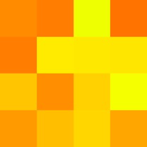
(a)

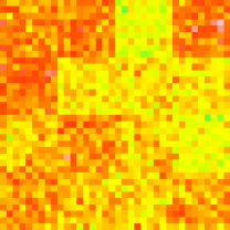
(b)

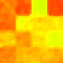
(c)

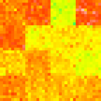
(d)

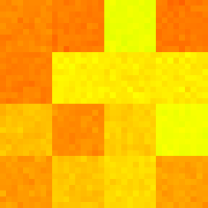
(e)

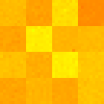
(f)

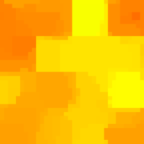
(g)

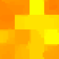
(h)

(i)

Figure 1. Simulation results for band $132$. (1a) Simulated hypercube before adding noise, (1b) Simulated hypercube after adding noise, (1c) Median denoising, (1d) Wiener denoising, (1e) Lee and Seung’s NMF used for denoising, (1f) SPA used for denoising, (1g) TV denoising with $\lambda_{s}=0.05$, and $\lambda_{t}=0$, (1h) TV denoising with $\lambda_{s}=0.05$, and $\lambda_{t}=0.01$, (1i) NMF-TV denoising with $\lambda_{s}=2.0$, and $\lambda_{t}=0.1$.

We were able to add TV regularization to the ADMM algorithm for NMF without slowing it down significantly. Resulting unmixings seem to benefit from introduced regularization.

To illustrate the denoising techniques proposed in this article, we generate a synthetic hypercube, and apply the $3$-dimensional TV denoising introduced in Section 2, and the NMF-TV algorithm from Section 3. NMF was not designed to remove noise. Its goal is to recover non-negative factors from a matrix. However, these factors are usually not unique, and can be quite different from the ones used to generate an example. Instead of assessing factors, we therefore focus on their product.

We generate a cube consisting of $16$ homogenous regions, each consisting of a randomly chosen mixture of $5$ randomly chosen spectrums in the USGS 1995 Library. We then add white noise, and try out our techniques.

More precisely, we start by building true endmembers matrix $W_{0}\in\mathbb{R}^{224\times 5}$ by stacking up $5$ endmembers randomly selected amongst the $498$ ones available in the library. We then build a first abundance matrix ${H_{0}}\in\mathbb{R}^{5\times 16}$ where every column is randomly drawn from a Dirichlet distribution. The matrix product $W_{0}H_{0}$ defines a matrix $M_{0}\in\mathbb{R}^{224\times 16}$ whom we fold into hypercube $\mathcal{M}_{0}\in\mathbb{R}^{4\times 4\times 224}$. To induce spatial regularity, we then replace each pixel $x$ of $\mathcal{M}_{0}$ by a $9\times 9$ block of copies of $x$. We get a cube of size ${36\times 36\times 224}$. We finally obtain hypercube $\mathcal{M}$ by adding gaussian noise.

$$\mathcal{M}=\mathcal{M}_{0}+\mathcal{N},$$

where every coefficient of $\mathcal{N}\in\mathbb{R}^{36\times 36\times 224}$ was randomly chosen according to the centered normal distribution.

We compare proposed techniques with $4$ relatively common algorithms, a median filter, a Wiener filter, and two $NMF$ algorithms : the seminal multiplicative update scheme from Lee and Seung [10], and the Successive Projection Algorithm (SPA) described by Gillis in [5]. The median filter replaces each pixel by the median of its $3\times 3\times 3$ neighborhood. The Wiener filter changes every pixel value $x$ according to

(18) $$y=\begin{cases}\frac{\sigma^{2}}{\sigma_{x}^{2}}m_{x}+\left(1-\frac{\sigma^{2}}{\sigma_{x}^{2}}\right)x\text{ if }\sigma_{x}^{2}\geq\sigma^{2},\\ m_{x}\text{ if }\sigma_{x}^{2}<\sigma^{2},\\ \end{cases}$$

where $m_{x}$ and $\sigma_{x}$ are the local mean and variance of the $3\times 3\times 3$ neighborhood of pixel $x$.

The median filter, Wiener filter and TV filter all give a result that we can directly compare to our synthesized example. The NMF algorithms results consist of two factors $W$ and $H$. We use their product $WH$ for comparisons.

ADMM parameter $\rho$ can theoretically be set to any value without compromising convergence. In practice, a good choice for $\rho$ is important, as it has an influence on the algorithm’s speed. We experimentally determined that setting $\rho=10$ allows our algorithm to converge reasonably fast. Parameters $\lambda$ and $\rho$ controlling the desired strength of TV-regularization were also set experimentally.

Results are displayed in Figure 1. Only one slice of the resulting hypercubes is displayed. The median and Wiener filter are not able to recover precisely the boundaries of every region as can be seen in Figure 1c and 1d. The classical NMF algorithms are not designed specifically with denoising in mind. However, their result displayed in Figure 1e and 1f show that they are quite successful at recovering sharp boundaries between every region. They however fail at producing smooth regions. Figure 1g results from a spatial only TV regularization, whereas Figure 1h is regularized by spatial–spectral TV. A careful comparison of both figures reveals that adding a spectral component to the TV denoising algorithm described in Section 2 seems to slightly improve the result. The NMF-TV algorithm recovers almost perfectly the original cube, as can be seen in Figure 1i.

To conclude, we state an interesting direction for future research. The base ingredient we used throughout our paper is a simple ADMM algorithm. We could instead try to use the Nesterov accelerated scheme described by Goldstein et al. in [6]. This would most likely speed up convergence.

Appendix

For an order $3$ tensor $\mathcal{T}\in\mathbb{R}^{m\times n\times o}$ the mode $1$-fiber corresponding to indices $(j,k)$ is the vector $(T_{i,j,k})_{1\leq i\leq m}$, the $2$-fiber corresponding to $(i,k)$ is defined as $(T_{i,j,k})_{1\leq j\leq n}$ and mode $3$-fibers are defined similarly as $(T_{i,j,k})_{1\leq k\leq n}$. Mode $n$ matricization, also known as unfolding, of tensor $\mathcal{T}$ transforms a tensor of any order in a matrix, by stacking its $n$-fibers in a precise order. The mode $k$ unfolding of tensor $\mathcal{T}$ is denoted $T^{(k)}$. A mode $n$ tensor contraction with a matrix is the generalization of the usual matrix product. The notion is probably better understood through an example. Let $\mathcal{T}$ be an order $3$ tensor, and $X$ be a matrix. The mode $2$ contraction of $\mathcal{T}$ and $X$, denoted $\mathcal{T}\times_{2}X$ is defined as

$$\left(\mathcal{T}\times_{2}X\right)_{i,l,k}=\sum_{l}T_{i,l,k}X_{l,j}.$$

Tensor contractions, unfoldings, and matrix product are linked by the following property :

$$\mathcal{U}=\mathcal{T}\times_{k}X\Leftrightarrow U^{(k)}=XT^{(k)}.$$

Multiple tensor contractions can be expressed with Kronecker products, thanks to one of its fundamental properties

$$\left(B^{T}\otimes A\right)\mbox{vec}(X)=\mbox{vec}(AXB)=\mbox{vec}(C).$$

This fact can be used to prove that the following propositions are equivalent :

1. $\mathcal{Y}=\mathcal{X}\times_{1}A^{1}\times_{2}A^{2}\times_{3}\cdots\times_{n}A^{n},$

2. $Y^{(k)}=A^{k}X^{(k)}\left(A^{n}\otimes\cdots\otimes A^{k+1}\otimes A^{k-1}\otimes\cdots\otimes A^{1}\right)^{T},$

3. $\mbox{vec}(Y^{(k)})=\left(A^{n}\otimes\cdots\otimes A^{k+1}\otimes A^{k-1}\otimes\cdots\otimes A^{1}\otimes A^{k}\right)\mbox{vec}(X^{(k)}).$

Last property lets us derive successively to the vectorization of Equation (11) in Section 2 :

$$B^{(1)}=(I_{mno}+\rho L_{o}\otimes I_{n}\otimes I_{m}+\rho I_{o}\otimes L_{n}\otimes I_{m}+\rho I_{o}\otimes I_{n}\otimes L_{m})X^{(1)}.$$

Kronecker sums are usually defined by

$$A\oplus B=A\otimes I_{n}+I_{m}\otimes B.$$

This definition can be extended to

$$A\oplus B\oplus C=A\otimes I_{n}\otimes I_{k}+I_{m}\otimes B\otimes I_{k}+I_{m}\otimes I_{n}\otimes C.$$

Note that Kronecker sums are associative but do not commute.

A useful fact about Kronecker sums and products is that they behave well with eigenvalue decompositions. Specifically, if $A=Q_{A}D_{A}Q_{A}^{T}$ and $B=Q_{B}D_{B}Q_{B}^{T}$ are the eigenvalue decompositions of matrices $A$ and $B$, then

$$A\otimes B=(Q_{A}\otimes Q_{B})(D_{A}\otimes D_{B})(Q_{A}\otimes Q_{B})^{T},$$

$$A\oplus B=(Q_{A}\otimes Q_{B})(D_{A}\oplus D_{B})(Q_{A}\otimes Q_{B})^{T},$$

are the respective eigen-decompositions of $A\otimes B$ and $A\oplus B$.

References

- [1] Hemant Kumar Aggarwal and Angshul Majumdar, Hyperspectral image denoising using spatio-spectral total variation, IEEE Geoscience and Remote Sensing Letters 13 (2016), no. 3, 442–446.
- [2] Sanjeev Arora, Rong Ge, Ravindran Kannan, and Ankur Moitra, Computing a nonnegative matrix factorization–provably, Proceedings of the forty-fourth annual ACM symposium on Theory of computing, ACM, 2012, pp. 145–162.
- [3] Christian Bauckhage, A purely geometric approach to non-negative matrix factorization., LWA, 2014, pp. 125–136.
- [4] Stephen Boyd, Neal Parikh, Eric Chu, Borja Peleato, and Jonathan Eckstein, Distributed optimization and statistical learning via the alternating direction method of multipliers, Foundations and Trends in Machine Learning 3 (2011), no. 1, 1–122.
- [5] Nicolas Gillis, The why and how of nonnegative matrix factorization, Regularization, Optimization, Kernels, and Support Vector Machines 12 (2014), 257.
- [6] Tom Goldstein, Brendan O’Donoghue, Simon Setzer, and Richard Baraniuk, Fast alternating direction optimization methods, SIAM Journal on Imaging Sciences 7 (2014), no. 3, 1588–1623.
- [7] Patrik O Hoyer, Non-negative matrix factorization with sparseness constraints, The Journal of Machine Learning Research 5 (2004), 1457–1469.
- [8] Marian-Daniel Iordache, José M Bioucas-Dias, and Antonio Plaza, Total variation spatial regularization for sparse hyperspectral unmixing, Geoscience and Remote Sensing, IEEE Transactions on 50 (2012), no. 11, 4484–4502.
- [9] Vijay Krishnamurthy and Alexandre d’Aspremont, Convex algorithms for nonnegative matrix factorization, arXiv preprint arXiv:1207.0318 (2012).
- [10] Daniel D Lee and H Sebastian Seung, Algorithms for non-negative matrix factorization, Advances in neural information processing systems, 2001, pp. 556–562.
- [11] José MP Nascimento and José MB Dias, Vertex component analysis: A fast algorithm to unmix hyperspectral data, IEEE transactions on Geoscience and Remote Sensing 43 (2005), no. 4, 898–910.
- [12] Michael K Ng, Raymond H Chan, and Wun-Cheung Tang, A fast algorithm for deblurring models with neumann boundary conditions, SIAM Journal on Scientific Computing 21 (1999), no. 3, 851–866.
- [13] Leonid I Rudin, Stanley Osher, and Emad Fatemi, Nonlinear total variation based noise removal algorithms, Physica D: Nonlinear Phenomena 60 (1992), no. 1, 259–268.
- [14] Stephen A Vavasis, On the complexity of nonnegative matrix factorization, SIAM Journal on Optimization 20 (2009), no. 3, 1364–1377.
- [15] R Warren and S Osher, Hyperspectral unmixing by the alternating direction method of multipliers, Inverse Problems and Imaging 14 (2015), no. 3, 00–00.
- [16] Junfeng Yang, Wotao Yin, Yin Zhang, and Yilun Wang, A fast algorithm for edge-preserving variational multichannel image restoration, SIAM Journal on Imaging Sciences 2 (2009), no. 2, 569–592.
- [17] Yin Zhang, An alternating direction algorithm for nonnegative matrix factorization, Rice Technical Report (2010).