Instabilities of a U(1) quantum spin liquid in disordered non-Kramers pyrochlores

Abstract

Quantum spin liquids (QSLs) are exotic phases of matter exhibiting long-range entanglement and supporting emergent gauge fields. A vigorous search for experimental realizations of these states has identified several materials with properties hinting at QSL physics. A key issue in understanding these QSL candidates is often the interplay of weak disorder of the crystal structure with the spin liquid state. It has recently been pointed out that in at least one important class of candidate QSLs - pyrochlore magnets based on non-Kramers ions such as Pr³⁺ or Tb³⁺- structural disorder can actually promote a $U(1)$ QSL ground state. Here we set this proposal on a quantitative footing by analyzing the stability of the QSL state in the minimal model for these systems: a random transverse field Ising model. We consider two kinds of instability, which are relevant in different limits of the phase diagram: condensation of spinons and confinement of the $U(1)$ gauge fields. Having obtained stability bounds on the QSL state we apply our results directly to the disordered candidate QSL Pr₂Zr₂O₇. We find that the available data for currently studied samples of Pr₂Zr₂O₇ is most consistent with it a ground state outside the spin liquid regime, in a paramagnetic phase with quadrupole moments near saturation due to the influence of structural disorder.

Experimental realizations of Quantum Spin Liquid (QSL) states are the goal of a long-running research effort lee08 ; balents10 . Interest in QSLs stems from their ability to support fractional excitations, emergent gauge fields and large-scale quantum entanglement savary17-RMP80 ; zhou17 . Several candidate QSLs are known and one key subset of these is found amongst pyrochlore oxides R₂M₂O₇ gardner10 ; gingras14 . The geometrical frustration of the pyrochlore lattice famously gives rise to spin ice- a classical spin liquid with magnetic monopole excitations- in Ho and Dy based pyrochlores harris97 ; castelnovo08 ; castelnovo12 . The theoretical result that a spin ice imbued with quantum fluctuations can host a $U(1)$ QSL with emergent photons hermele04 ; banerjee08 ; savary12 ; shannon12 ; benton12 ; hao14 ; kato15 ; mcclarty15 ; chen16 has fueled interest in spin-ice-like systems with stronger quantum effects ross11 ; chang12 ; tokiwa15 ; thompson-arXiv ; fennell12 ; kermarrec15 ; takatsu16 ; hallas15 ; sibille15 ; zhou08 ; kimura13 ; petit16-NatPhys12 ; sibille16 ; anand16 ; sibille17-arXiv .

A recurrent issue in these investigations is the role of quenched disorder ross12 ; taniguchi13 ; arpino17 ; mostaed17 . Recently savary17-PRL118 , Savary and Balents have demonstrated that for pyrochlores based on non-Kramers ions weak structural disorder can actually promote the QSL ground state. This is because structural imperfections around the magnetic sites act as transverse fields on the low energy effective $S=1/2$ degrees of freedom. These transverse fields induce tunneling between classical spin ice ground states, which stabilizes the $U(1)$ QSL. Experiments confirm the presence of these transverse fields in the candidate quantum spin ice Pr₂Zr₂O₇ wen17 ; martin17 suggesting the possibility of a disorder-induced QSL ground state.

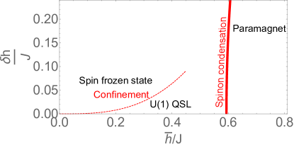
Figure 1: Instabilites of the $U(1)$ QSL in the random transverse field Ising model on the pyrochlore lattice [Eq. (5)]. There are two instabilities which appear upon increasing the average strength $\bar{h}$ and width $\delta h$ of the distribution of transverse fields. The condensation of spinons leads to a trivial paramagnetic phase, and the threshold for this instablity can be calculated by calcularing the spinon energy perturbatively [Eq. (15)]. The second instability is to confinement of the $U(1)$ gauge field, leading to a glassy state with frozen magnetic moments. The threshold for this instability occurs along a line $\delta h=\alpha\bar{h}^{3}$, for small $\delta h/J,\bar{h}/J$. The coefficient $\alpha$ depends on the details of the distribution of transverse fields, the figure shows a sketch with $\alpha=1$.

This Letter addresses two questions. Firstly, what is the extent of the QSL phase in the minimal model for non-Kramers pyrochlores with weak structural disorder? Secondly, do currently studied samples of Pr₂Zr₂O₇ fall within this QSL phase?

The first of these questions is answered by considering two instabilities of the $U(1)$ QSL: spinon condensation and confinement. The threshhold for each can be calculated in perturbation theory. Fig. 1 shows the results of this calculation.

Determining to which phase Pr₂Zr₂O₇ belongs requires parameterizing a model for this material. We do this by comparing available thermodynamic data to Numerical Linked Cluster (NLC) rigol06 ; rigol07 ; tang13 calculations. Our model suggests current samples of Pr₂Zr₂O₇ fall within a paramagnetic phase, with $4f$ quadrupole moments nearly saturated by the effective transverse fields. Exact Diagonalization (ED) calculations suggest this conclusion is consistent with scattering experiments showing an excitation continuum and broadened, spin-ice-like, correlations at low energies kimura13 ; petit16-PRB94 .

Stability regime of the QSL- We consider a minimal model for non-Kramers pyrochlores where the degeneracy of the ground crystal electric field (CEF) doublet is lifted by local deviations from $D_{3d}$ site symmetry. We assume that the gap to higher energy CEF states is large such that the only relevant degrees of freedom are Pauli matrices $\vec{\sigma}_{i}$ describing the two states of the ground doublet. Due to the symmetry of non-Kramers doublets onoda10 ; onoda11 on the pyrochlore lattice, the magnetic moment on site $i$ points only along the local-axis $\hat{{\bf z}_{i}}$ joining the centers of the pyrochlore tetrahedra sharing the site

$${\bf m}_{i}=\mu_{\sf eff}\sigma^{z}_{i}\hat{\bf z}_{i}$$ (1)

where $\mu_{\sf eff}$ is the effective moment size. Nearest-neighbor Ising interactions

$$\mathcal{H}_{\sf SI}=J\sum_{\langle ij\rangle}\sigma^{z}_{i}\sigma^{z}_{j}$$ (2)

with $J>0$ favour spin-ice-like states in which the total value of $\sigma^{z}_{i}$ vanishes on every tetrahedron in the lattice

$$\sum_{i\in t}\sigma^{z}_{i}=0\quad\forall\ \text{tetrahedra}\ t$$ (3)

The transverse pseudospin operators $\sigma^{x,y}_{i}$ are time-reversal invariant and cannot contribute to the magnetic moment. A finite value of these operators corresponds instead to a finite quadrupole moment onoda10 ; onoda11 . The time-reversal invariance of $\sigma^{x,y}_{i}$ allows them to couple linearly to lattice imperfections which lift the local $D_{3d}$ symmetry savary17-PRL118 . These imperfections thus act as a transverse field on $\sigma_{i}$

$$\mathcal{H}_{\sf TF}=-\sum_{i}h_{i}\sigma^{x}_{i}$$ (4)

where we have used local coordinate transformations on $\sigma^{\alpha}_{i}$ such that the coupling is always to $\sigma^{x}_{i}$ savary17-PRL118 . The transverse fields $h_{i}$ are distributed on the interval $[0,\infty]$ and we assume them to be uncorrelated in space $\overline{h_{i}h_{j}}=\overline{h_{i}}\ \ \overline{h_{j}}$. We use $\overline{x}$ to denote the average of $x$ over disorder realizations, reserving $\langle x\rangle$ for quantum statistical averages at fixed disorder realization.

The minimal model for non-Kramers pyrochlores with weak structural disorder is thus a random transverse field Ising model savary17-PRL118

$$\mathcal{H}_{\sf RTFIM}=\mathcal{H}_{\sf SI}+\mathcal{H}_{\sf TF}.$$ (5)

For weak, uniform, $h_{i}$ the ground state is a $U(1)$ QSL, while for $h_{i}\gg J$ a trivial paramagnetic state is expected savary17-PRL118 . The transition between these phases occurs via condensation of the gapped spinon excitations of the $U(1)$ QSL savary17-PRL118 ; roechner16 . Below, we use perturbation theory to estimate the threshhold for this transition. We then consider an alternative, confinement, instability of the QSL which leads to a frozen moment state.

In the limit $h_{i}=0$ a spinon corresponds to a tetrahedron $t$ where Eq. (3) is violated, with $\sum_{i\in t}\sigma^{z}_{i}=\pm 2$ and a gap $\Delta_{0}=2J$. To calculate the gap in the presence of disordered transverse fields we consider a state containing $M$ spinons. We take $1\ll M\ll N_{t}$, where $N_{t}$ is the number of tetrahedra in the lattice, such that the spinon density is low and spinon interactions may be neglected. Using second order perturbation theory we obtain an effective Hamiltonian acting amongst these $M$ spinon states

$$\mathcal{H}_{\sf eff}^{(M)}=E_{0}^{\sf cl}+M\Delta_{0}+\mathcal{H}_{1}^{(M)}+\mathcal{H}_{2}^{(M)}$$ (6)

$$\mathcal{H}_{1}^{(M)}=\mathcal{P}_{M}\mathcal{H}_{\sf TF}\mathcal{P}_{M}$$ (7)

$$\mathcal{H}_{2}^{(M)}=-\mathcal{P}_{M}\mathcal{H}_{\sf TF}\frac{\mathcal{Q}_{M}}{\mathcal{H}_{\sf SI}-(E_{0}^{\sf cl}+M\Delta_{0})}\mathcal{H}_{\sf TF}\mathcal{P}_{M}\quad$$ (8)

where $E_{0}^{\sf cl}=-NJ$, $\mathcal{P}_{M}$ projects onto the manifold of states with $M$ spinons and $\mathcal{Q}_{M}$ projects onto its orthogonal complement.

To find the lowest energy state for $M$ spinons we use the fact that for $1\ll M\ll N_{t}$ the column sum of $\mathcal{H}_{\sf eff}^{(M)}$ is approximately constant kourtis16 ; wan16 . To see this, consider first $\mathcal{H}_{1}^{(M)}$, which allows each spinon to hop to three of its four neighboring tetrahedra. The column sum of $\mathcal{H}_{1}^{(M)}$ is

$$\sum_{\alpha}\left(\mathcal{H}_{1}^{(M)}\right)_{\alpha\beta}=-\sum_{i\in{\text{flippable}}}h_{i}$$ (9)

For sparse spinons $M\ll N$ there are $3M$ flippable spins and

$$\sum_{\alpha}\left(\mathcal{H}_{1}^{(M)}\right)_{\alpha\beta}=-3M\frac{1}{3M}\sum_{i\in{\text{flippable}}}h_{i}=-3M\overline{h}$$ (10)

where we have used the fact that $M\gg 1$ and the assumption that $h_{i}$ are uncorrelated on different sites.

The second order part of the effective Hamiltonian $\mathcal{H}_{2}^{(M)}$, contains a diagonal contribution which is constant for $1\ll M\ll N$

$$\left(\mathcal{H}_{2}^{(M)}\right)_{\alpha\alpha}=-\frac{N_{t}}{2J}\overline{h^{2}}+\frac{7M}{8J}\overline{h^{2}}$$ (11)

coming from virtual processes which flip the same spin twice. The off-diagonal part of $\left(\mathcal{H}_{2}^{(M)}\right)_{\alpha\beta}$ enables spinons to hop to 6 out of their 12 second-nearest-neighbor tetrahedra by flipping two spins $k,l$ with matrix element $-\frac{h_{k}h_{l}}{4J}$. Since each $M$ spinon configuration can tunnel to the same number of other $M$ spinon configurations we find that the column sum of the second order Hamiltonian is also approximately constant:

$$\sum_{\alpha}\left(\mathcal{H}_{2}^{(M)}\right)_{\alpha\beta}=-\frac{N_{t}}{2J}\overline{h^{2}}+\frac{7M}{8J}\overline{h^{2}}-\frac{3M}{2J}\overline{h}^{2}$$ (12)

Since $\mathcal{H}_{\sf eff}^{(M)}$ [Eq. (6)] has approximately constant column sum, and negative off-diagonal matrix elements its ground state must be an equal weight, Rokhsar-Kivelson-like, superposition of all configurations containing $M$ spinons kourtis16 ; wan16 ; rokhsar88

$$|\phi_{M}\rangle=\frac{1}{\sqrt{\mathcal{N}_{M}}}\sum_{|\alpha\rangle\in\{|M\rangle\}}|\alpha\rangle$$ (13)

where $\mathcal{N}_{M}$ is the number of such configurations.

Using this wave function and Eq. (6) to calculate the energy gives

$$E(M)=E_{0}^{\sf cl}-\frac{N_{t}\overline{h^{2}}}{2J}+M\left(2J-3\overline{h}+\frac{7\delta h^{2}-5\overline{h}^{2}}{8J}\right)\ \ \ \quad$$ (14)

where $\delta h=\sqrt{\overline{h^{2}}-\overline{h}^{2}}$.

When the coefficient of $M$ in Eq. (14) becomes negative it becomes favorable for spinons to proliferate and condense. Stability of the QSL against spinon condensation thus requires

$$2J-3\overline{h}+\frac{7}{8J}\delta h^{2}-\frac{5\overline{h}^{2}}{8J}>0$$ (15)

as plotted in Fig. 1. Beyond this line the system gives way to a trivial paramagnetic ground state.

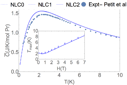
(a)  Heat capacity

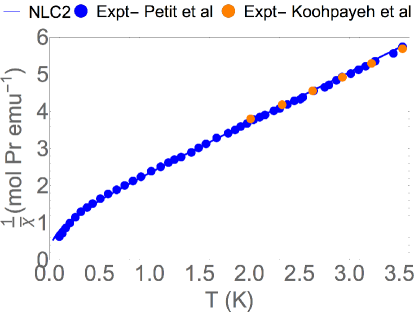
(b)  Inverse susceptibility

Figure 2: Establishing a model for Pr₂Zr₂O₇. NLC calculations for the random transverse field Ising model [Eq. (5)] using $J=0.02$ meV, effective moment $\mu_{\sf eff}=2.45\mu_{B}$ and a Lorentzian distribution of transverse fields with width $\Gamma=0.2$ meV give a good description of the heat capacity [(a)] and inverse susceptibility [(b)]. Experimental results for the heat capacity are extracted footnote1 from Ref. petit16-PRB94 and results for the susceptibility from Refs. petit16-PRB94 ; koohpayeh14 . The inset of (a) shows the development of the temperature of the specific heat maximum under a magnetic field applied along the [110] direction, compared between NLC calculations and data from Ref. petit16-PRB94 . The heat capacity of isostructural La₂Zr₂O₇ matsuhira09 was subtracted from the data from petit16-PRB94 to remove the phonon contribution. Calculations are averaged over $10^{6}$ disorder realizations.

We can compare the result of Eq. (15) to the phase boundary of the uniform transverse field model ($\delta h=0$) found in Ref. roechner16 . Inserting $\delta h=0,\overline{h}=h$ into Eq. (15) we find the critical value for $h$ is $h_{c}\approx 0.593J$, close to the $h_{c}\approx 0.602J$ obtained from high field expansion in roechner16 . The agreement with the results of roechner16 for the uniform case suggests that the second order calculation is sufficient, at least when $\delta h$ is small.

In deriving Eq. (15) we have considered $M$ spinon states with $1\ll M\ll N$, to justify inserting averaged matrix elements in Eqs. (10)-(12). One may wonder what happens for states with small spinon number $M\sim 1$. In this case a lower energy may be obtained by restricting spinons to small subregions with untypically large values of $h_{i}$. The condensation of spinons within these subregions can thus occur before the bulk instability predicted by Eq. (15), leading to a Griffiths phase in which most of the system remains in the QSL state but there are rare paramagnetic regions savary17-PRL118 . The Griffiths phase is difficult to address analytically but could be be identified in simulation via spinon zero modes appearing at the boundaries of the paramagnetic regions savary17-PRL118 .

While Eq. (15) establishes a bulk stability bound against spinon condensation, there is another relevant instability for the QSL. This second instability corresponds to the condensation of the “magnetic” monopole charge, leading to a confinement transition chen16 . Unlike the spinons, the magnetic monopole is an excitation within the ice manifold, so this instability should be addressed using degenerate perturbation theory within the classical ground states. A perturbative treatment of $\mathcal{H}_{\sf TF}$ within the ground state manifold of $\mathcal{H}_{\sf SI}$ leads to a term at fourth order which makes the Ising exchange interactions bond dependent

$$J\to J+\delta J_{ij},\ \delta J_{ij}=\frac{h_{i}^{2}h_{j}^{2}}{48J^{3}}$$ (16)

(see Supplemental Material for details). The ground state of the bond dependent Ising Hamiltonian will be some frozen state of $\sigma_{i}^{z}$ which depends on the disorder realization. Such a ground state corresponds to a confined phase of the $U(1)$ gauge theory.

In the limit of uniform transverse fields ($\delta h=0$) this term becomes a constant and the leading non-trivial term is then a sixth order ring exchange $g\sim h^{6}$ which stablizies the $U(1)$ QSL. At finite $\delta h$, the transition between the QSL and confined phases must occur when $g\sim\delta J$, which gives a phase boundary

$$\delta h=\alpha\bar{h}^{3}$$ (17)

with $\alpha$ depending on the details of the transverse field distribution. Determination of $\alpha$ for a given type of distribution requires a numerical study beyond the scope of this work.

Modeling Pr₂Zr₂O₇- We now seek to establish a model for the candidate QSL Pr₂Zr₂O₇, and determine its location on the phase diagram. In Ref. wen17 the distribution of $h_{i}$ arising in a sample of Pr₂Zr₂O₇ was characterized by analyzing inelastic neutron scattering results in an applied magnetic field. The result was a Lorentzian distribution

$$p(h)=\frac{2\Gamma}{\pi}\frac{1}{\Gamma^{2}+h^{2}},\quad h\in[0,\infty]$$ (18)

with $\Gamma=0.27$meV.

Inspired by this we have compared thermodynamic data from other samples of Pr₂Zr₂O₇ petit16-PRB94 ; bonville16 ; koohpayeh14 to NLC calculations using the Hamiltonian in Eq. (5), with a Lorentzian distribution of transverse fields (see Supplemental Material for details). The NLC expansion is a means of estimating quantities in the thermodynamic limit from a series of diagonalizations of small clusters rigol06 ; rigol07 ; tang13 , which has been used successfully for other pyrochlores singh12 ; applegate12 ; hayre13 ; jaubert15 . Disorder averages can be taken term by term in the expansion tang15-PRB91 ; tang15 . Calculations are done using zeroth (NLC0), first (NLC1) and second (NLC2) order expansions, incorporating clusters of 1 site, 1 tetrahedron and two tetrahedra respectively. The interaction strength $J$, distribution width $\Gamma$ and effective moment $\mu_{\sf eff}$ are treated as adjustable parameters. We have focussed on obtaining agreement with thermodynamic data from Refs. petit16-PRB94 ; bonville16 , but the quantitatively similar heat capacity curves obtained elsewhere kimura13 ; koohpayeh14 suggest that the model we obtain should be approximately valid for other currently studied samples.

Agreement with heat capacity and susceptibility data is obtained in the parameter range $J=(0.020\pm 0.005)$meV $\Gamma=(0.20\pm 0.01)$meV, $\mu_{\sf eff}=(2.45\pm 0.05)\mu_{B}$, as shown in Figure 2(a)-(b). Our fits capture the antiferromagnetic Curie-Weiss behavior in spite of having a spin-ice like $J>0$. They also capture the broad maximum in the specific heat and its evolution as a function of applied field [inset of Fig. 2(a)].

Despite obtaining a narrower distribution of transverse fields than quoted in wen17 , our fitted model gives a reasonable description of the neutron scattering data from that study. This is shown in Fig. 3, where we compare the disorder averaged on-site correlation function

$$\overline{C}_{ii}(\omega)=\overline{\sum_{|\alpha\rangle}|\langle 0|\sigma^{z}_{i}|\alpha\rangle|^{2}\delta(\omega-E_{\alpha})}$$ (19)

for the central spin of a 2-tetrahedron cluster with ${\bf q}$-integrated scattering data from Ref. wen17 . The model overestimates the scattering close to the Zeeman energy at each value of field, but agrees closely with the high energy scattering, and agrees qualitatively with the form of the lower energy scattering. Differences between the model and experimental data may be attributable to interactions not included in the simple model Eq. (5), spatial correlations in the transverse field distribution wen17 and variation between samples.

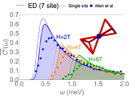
Figure 3: On-site correlation function $\overline{C}_{ii}(\omega)$ calculated for three values of external magnetic field along the [100] direction. Calculations are made using ED on the 7-site cluster shown in the inset, using parameters $J=0.02$meV and $\Gamma=0.2$meV. $C_{ii}(\omega)$ is calculated for the central spin of the cluster. The dashed lines show a single site calculation (i.e. neglecting interactions $J$) and the calculations are compared with ${\bf q}$ integrated data from Ref. wen17 , which are multiplied by an overall scale factor. The calculation has been averaged over $2\times 10^{5}$ disorder realizations and convoluted with a Gaussian of Full Width at Half Maximum (FWHM) =0.11 meV to mimic experimental resolution.

What does this model suggest about Pr₂Zr₂O₇? A difficulty with the Lorentzian distribution [Eq. (18)] is that its moments $\overline{h},\overline{h^{2}}$ are not well defined. This inhibits direct application of the stability criterion (15). We can circumvent this issue by applying a finite cut-off $h_{max}$ to the distribution in Eq. (18) and observing the trajectory of $\overline{h},\delta h$ as the cut-off is increased, while keeping $J=0.02$meV and $\Gamma=0.2$meV. Upon the increasing the cut-off from $h_{max}=0$, the model crosses into the paramagnetic region of Fig. 1 for cut-offs as low as $h_{max,c}=0.025$meV. Since the distribution of transverse fields in Pr₂Zr₂O₇ certainly extends far beyond this point, we should expect Pr₂Zr₂O₇ to fall deep within the paramagnetic phase of the model. This agrees with both NLC and 16-site ED calculations which predict a nearly saturated ground state expectation value of $\overline{\langle\sigma_{x}\rangle}\approx 0.98$ with $J=0.02$meV and $\Gamma=0.20$meV.

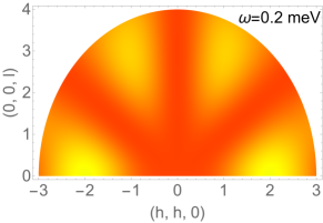
Figure 4: Calculation of the inelastic structure factor at $\omega=0.2$meV for Pr₂Zr₂O₇ [Eq. (20) ]. The calculation uses real space correlators $\overline{C}_{ij}(\omega)$ calculated from Exact Diagonalization of Eq. (5) on a 16 site cubic cluster, with $J=0.02$meV and a Lorentzian distribution of transverse fields [Eq. (18)] with $\Gamma=0.2$meV. Calculations are averaged over 300 realisations of disorder and convoluted with a Gaussian of FWHM =0.11 meV to mimic finite experimental resolution. This calculation reproduces the broadened remnants of spin-ice like correlations observed at finite energy in Pr₂Zr₂O₇ kimura13 ; petit16-PRB94 .

A natural question at this point is whether this conclusion can be reconciled with inelastic neutron scattering experiments kimura13 ; petit16-PRB94 . To address this we have calculated disorder averaged real space correlation functions, $\overline{C}_{ij}(\omega)$, up to third nearest neighbour in 16-site ED and combined them into a calculation of the dynamical structure factor for neutron scattering

$$S_{\mathbf{q}}(\omega)=\sum_{i,j}{\frac{e^{i\mathbf{q}\cdot({\bf r}_{i}-{\bf r}_{j})}\left(\hat{\bf z}_{i}\cdot\hat{\bf z}_{j}-(\hat{\bf z}_{i}\cdot\hat{\bf q})(\hat{\bf z}_{j}\cdot\hat{\bf q})\right)\overline{C}_{ij}(\omega)}{N}}\qquad$$ (20)

Using our model parameters to calculate this at finite energy $\omega=0.2$meV, we obtain a similar pattern to that observed in Refs. kimura13 ; petit16-PRB94 , namely broadened remnants of spin-ice like correlations. This suggests that neutron scattering observations on Pr₂Zr₂O₇ can be reconciled with the paramagnetic state predicted here.

Conclusions- We have investigated the instabilities of the $U(1)$ QSL against spinon condensation and confinement in a model describing non-Kramers pyrochlore magnets with weak disorder. We have parameterized this model for currently studied samples of the Pr₂Zr₂O₇ and found that they most likely fall within the paramagnetic regime, a result consistent with available scattering data. An interesting direction for future research is to seek control of the transverse field distribution by varying experimental parameters in the synthesis procedure. If one can tune through the spinon condensation threshhold in this way, then not only the $U(1)$ QSL phase but also the topological quantum phase transition connecting the QSL to the paramagnetic phase become accessible. The determination of the phase boundary and the method of estimating model parameters from thermodynamics used in this work can aid in the fine tuning of samples through the phase transition.

Other Pr pyrochlores such as Pr₂Hf₂O₇ sibille16 ; anand16 and Pr₂Sn₂O₇ zhou08 are of great interest, particularly given recent experimental results indicating the possible existence of emergent photons in Pr₂Hf₂O₇ sibille17-arXiv . Further work is needed to determine whether these materials realize the $U(1)$ QSL.

Acknowledgments The author acknowledges useful discussions with Bella Lake, Kate Ross, Alexandros Samartzis, Nic Shannon and Jiajia Wen.

I Supplemental Material: Instabilities of a $U(1)$ quantum spin liquid in disordered non-Kramers pyrochlores

II Details of Numerical Linked Cluster Calculations

Here we give some details of the Numerical Linked Cluster (NLC) calculations presented in the main text. A pedagogical introduction to NLC expansions is given in tang13 .

In Numerical Linked Cluster expansions an extensive quantity $\mathcal{O}$ divided by the number of sites $N$, is calculated as a sum over contributions from all clusters $c$ that can be embedded in the lattice

$$\frac{1}{N}\langle\mathcal{O}\rangle=\sum_{c}M(c)W(c).$$ (21)

$M(c)$ is the multiplicity of the cluster per site- i.e. how many times that cluster can be embedded in a lattice of $N$ sites, divided by $N$. $W(c)$ is the cluster weight defined as

$$W(c)=\langle\mathcal{O}\rangle_{c}-\sum_{s\subset c}W(s)$$ (22)

where $\langle\mathcal{O}\rangle_{c}$ is the expectation value of $\mathcal{O}$ on the cluster $c$, which is calculated from exact diagonalization. The sum in the second term is a sum of the weights of all the subclusters of $c$.

In our calculations we have used the series of clusters shown in Fig. 5, calculating the series up to second order. We have used clusters of 1, 4 and 7 sites and we denote them as $c_{1},c_{4},c_{7}$. The multiplicities of these clusters per site are

$$M(c_{1})=1,\quad M(c_{4})=\frac{1}{2}\quad M(c_{7})=1$$ (23)

and the weights for calculation of quantity $\mathcal{O}$ per site are

$$W(c_{1})=\langle\mathcal{O}\rangle_{c_{1}}$$

$$W(c_{4})=\langle\mathcal{O}\rangle_{c_{4}}-4\langle\mathcal{O}\rangle_{c_{1}}$$

$$W(c_{7})=\langle\mathcal{O}\rangle_{c_{7}}-2(\langle\mathcal{O}\rangle_{c_{4}}-4\langle\mathcal{O}\rangle_{c_{1}})-7\langle\mathcal{O}\rangle_{c_{1}}.$$ (24)

In the presence of disorder, disorder averaged quantities can be calculated by taking the disorder average term by term tang15 , i.e.

$$\frac{1}{N}\overline{\langle\mathcal{O}\rangle}=\sum_{c}M(c)\overline{W(c)}$$ (25)

$$\overline{W(c)}=\overline{\langle\mathcal{O}\rangle_{c}}-\sum_{s\subset c}\overline{W(s)}$$ (26)

(a)  Cluster $c_{1}$: One site

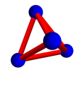
(b)  Cluster $c_{4}$: One tetrahedron

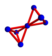
(c)  Cluster $c_{7}$: Two tetrahedra

Figure 5: Series of clusters used in NLC calculations in the main text.

For the calculations in the presence of an external [110] magnetic field [inset of Fig. 2(a) of main text], the reduction in point group symmetry due to the applied field means that the clusters $c_{1}$ and $c_{7}$ now have two inequivalent types which must be treated separately hayre13 .

III Optimization of model parameters for $\text{Pr}_{2}\text{Zr}_{2}\text{O}_{7}$

Here we describe the procedure used to optimize the model parameters $J,\Gamma,\mu_{\sf eff}$ to describe the thermodynamics of $\text{Pr}_{2}\text{Zr}_{2}\text{O}_{7}$ [Fig. 2 of main text].

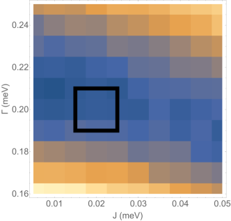
Figure 6: Total squared error of the fit to the zero-field heat capacity data of Ref. [petit16-PRB94, ], as a function of the width parameter $\Gamma$ and the Ising exchange $J$. Calculations were made for each value of $\Gamma,J$ using second-order NLC expansion and averaging over $10^{6}$ realizations of disorder. The best fits are obtained with $\Gamma\in[0.19,0.22]$ meV, $J<0.035$meV. In this limit the fit quality is only weakly dependent on $J$ which must be fixed using the susceptibility data [see Fig. 7]. The black square indicates the region where t where both$(\Delta_{C})^{2}$ and $(\Delta_{\chi^{-1}})^{2}$ are minimized, up to the accuracy of our calculations. This region constitutes our estimates of the model parameters [Eq. (29)].

To begin with we consider the zero-field heat capacity data in the temperature range $T\in[0.4,10]$K, which we have extracted from Ref. [petit16-PRB94, ]. For each value of the temperature we have subtracted the lattice specific heat based on the measurements for non-magnetic La₂Zr₂O₇ in matsuhira09 , to obtain the experimental magnetic heat capacity $C^{\sf mag,exp}(T)$.

We then calculate $\bar{C}(J,\Gamma,T)$ in second order NLC for a series of values of $J$ at intervals of $0.005$meV and $\Gamma$ at intervals of $0.01$ meV respectvely. The calculation is made using disorder averaging over $10^{6}$ realizations of disorder. Note that the zero field heat capacity is independent of the effective moment $\mu_{\sf eff}$.

For each value of $J$, $\Gamma$ we calculate the total squared error

$$\Delta_{C}^{2}=\frac{1}{N_{p}}\sum_{i}(C^{\sf mag,exp}_{i}(T_{i})-\bar{C}(J,\Gamma,T_{i}))^{2}$$ (27)

where the index $i$ runs over experimental data points $C^{\sf mag,exp}_{i}(T_{i})$ and $N_{p}=47$ is the number of data points used.

The results of this calculation are shown in Fig. 6. The best fits are obtained with distribution widths $\Gamma\in[0.19,0.22]$meV, and with $J<0.035$meV. This is a parameter regime where the heat capacity is dominated by the distribution of transverse fields, so the quality of fit is only very weakly dependent on $J$.

To fix $J$ and $\mu_{\sf eff}$ we turn to the inverse susceptiility data. Similarly to the treatment of the heat capacity we extract the experimental susceptibility $\frac{1}{\chi^{\sf exp}(T)}$ from Ref. petit16-PRB94 . We then calculate $\bar{\chi}^{-1}(J,\Gamma,\mu_{\sf eff},T)$ in second order NLC for the same parameter sets $J,\Gamma$ used to calculate the heat capacity in Fig. 6, averaging over $10^{6}$ realizations of disorder.. Initially we set $\mu_{\sf eff}=2.45\mu_{B}$ as found in Ref. petit16-PRB94 .

The total squared error for the inverse susceptibility is

$$\Delta_{\chi^{-1}}^{2}=\frac{1}{N_{p}}\sum_{i}\left(\frac{1}{\chi^{\sf exp}_{i}}(T_{i})-\bar{\chi}^{-1}(J,\Gamma,\mu_{\sf eff},T_{i})\right)^{2}$$ (28)

where $i$ runs over experimental data points $\frac{1}{\chi^{\sf exp}_{i}(T_{i})}$ and $N_{p}=51$ is the number of data points used.

$\Delta_{\chi^{-1}}^{2}$ is plotted as a function of $J,\Gamma$ with $\mu_{\sf eff}=2.45\mu_{B}$ in Fig. 7. There is a line of parameter sets which each give an approximately equally good fit, diagonally across the $(J,\Gamma)$ plane.

The black box plotted in Figs. 6 and 7 indicates the region which gives good agreement for both the heat capacity [Fig. 6] and inverse susceptibility.

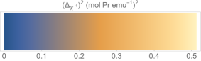
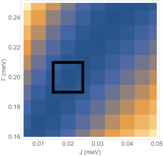
Figure 7: Total squared error of the fit to the inverse magnetic susceptbility data of Ref. [petit16-PRB94, ], as a function of the width parameter $\Gamma$ and the Ising exchange $J$. Here the effective magnetic moment is fixed to $\mu_{\sf eff}=2.45\mu_{B}$, in agreement with [petit16-PRB94, ]. Calculations were made for each value of $\Gamma,J$ using second-order NLC expansion and averaging over $10^{6}$ realizations of disorder. There is an extended minimum in $(\Delta_{\chi^{-1}})^{2}$ in the $(J,\Gamma)$ plane, running diagonally across the plot. The black square indicates the region where this minimum intersects the minimum in $(\Delta_{C})^{2}$ [Fig. 6]. This gives us our estimate of the model parameters [Eq. (29)].

Figure 8: Total squared error of the fit to the inverse magnetic susceptbility data of Ref. [petit16-PRB94, ], as a function of the Ising exchange $J$, for various values of $\mu_{\sf eff}$ and $\Gamma=0.20$ meV. Calculations were made for each value of $J,\mu_{\sf eff}$ using second-order NLC expansion and averaging over $10^{6}$ realizations of disorder. Error bars are statistical errors from the disorder average. Varying $\mu_{\sf eff}$ away from $\mu_{\sf eff}=2.45\mu_{B}$ results in a poorer fit to the data.

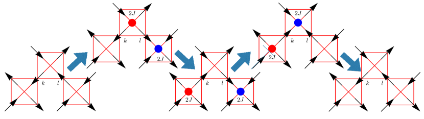
(a)  Antiferromagnetic bond $\sigma^{z}_{k}=-\sigma^{z}_{l}$

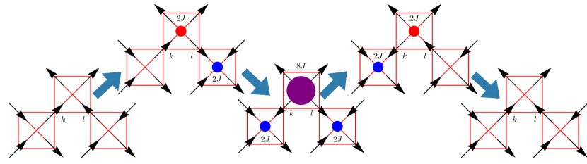
(b)  Ferromagnetic bond $\sigma^{z}_{k}=\sigma^{z}_{l}$

Figure 9: Processes contributing at fourth order in perturbation theory [Eq. (33)] on a bond $k,l$ in a spin ice state. The labels on the intermediate states, indicate the energy of each tetrahedron, relative to its ground state energy, in that state. These quantities appear in the denominator of the correction to the energy [Eq. (33)]. The resulting correction to the energy depends on whether the bond $k,l$ is antiferromagnetic [(a)] or ferromagnetic [(b)] in the initial state. The total correction to the energy for an antiferromagnetic bond arising from these processes is $\delta E_{\sf AFM}^{(4)}=-\frac{h_{k}^{2}h_{l}^{2}}{16J^{3}}$, whereas for a ferromagnetic bond it is $\delta E_{\sf FM}^{(4)}=-\frac{h_{k}^{2}h_{l}^{2}}{48J^{3}}$.

This region is delineated by

$$J=0.020\pm 0.005\ \text{meV}$$

$$\Gamma=0.20\pm 0.01\ \text{meV}$$ (29)

Lastly, we check the robustness of the parameter set against variations of the ordered moment $\mu_{\sf eff}$. The heat capacity does not depend on $\mu_{\sf eff}$ so we need only check the fit to the susceptibility. Fig. 8 shows $\Delta_{\chi^{-1}}^{2}$ as a function of $J$ for values of $\mu_{\sf eff}$ in the range $[2.35,2.55]\mu_{B}$, with $\Gamma=0.2$ meV. Moving away from $\mu_{\sf eff}=2.45\mu_{B}$ significantly reduces the quality of the optimum fit.

We estimate

$$\mu_{\sf eff}=2.45\pm 0.05\ \mu_{B}.$$ (30)

IV Confinement instability of the $U(1)$ QSL

Here we describe the perturbation theory calculation which leads to the result that the instability threshold for a confinement transition of the $U(1)$ gauge fields occurs along a line

$$\frac{\delta h}{J}\approx\alpha\left(\frac{\bar{h}}{J}\right)^{3}$$ (31)

with the coefficient $\alpha$ being dependent on the distribution of transverse fields.

The confinement transition is associated with the condensation of a dual monopole charge, and leads to a state with frozen Ising moments $\sigma^{z}_{i}$ chen16 . In the perturbative limit ${\bar{h}},{\delta h}\ll J$, the dual monopoles are excitations within the manifold of classical spin ice states. To address this instability, it is therefore appropriate to consider perturbation theory within the manifold of classical spin ice ground states.

Considering $\mathcal{H}_{\sf TF}$ [Eq. (4) of main text] as a perturbation to $\mathcal{H}_{\sf SI}$ [Eq. (2) of main text] within degenerate perturbation theory in the ice manifold, only even orders of the expansion are non-vanishing. At second order, there is only a trivial constant shift in the energy

$$\delta E^{(2)}=-\sum_{i}\frac{h_{i}^{2}}{4J}$$ (32)

which is independent of the configuration of $\sigma_{z}^{i}$.

For non-uniform transverse fields, there is a non-trivial contribution arising at fourth order. This contribution arises from virtual processes in which two neighbouring spins are flipped, creating excitations out of the ground state manifold, and then both are flipped back, thus returning to the original spin configuration [see Fig. 9]. Such processes generate an effective Hamiltonian, acting within the classical ground state manifold

$$\mathcal{H}^{g}_{(4)}=-\mathcal{P}_{\sf g}\mathcal{H}_{\sf TF}\left(\frac{\mathcal{Q}_{\sf g}}{\mathcal{H}_{\sf SI}-E_{0}^{\sf cl}}\mathcal{P}_{\sf g}\mathcal{H}_{\sf TF}\right)^{3}\mathcal{P}_{g}$$ (33)

where $\mathcal{P}_{\sf g}$ projects onto the classical ground state manifold and $\mathcal{Q}_{\sf g}$ projects onto its orthogonal complement.

For an antiferromagnetic bond $k,l$, with $\sigma^{z}_{k}=-\sigma^{z}_{l}$ the total contribution to the fourth order correction to the energy is

$$\delta E_{\sf AFM}^{(4)}=-\frac{h_{k}^{2}h_{l}^{2}}{16J^{3}}$$ (34)

while for a ferromagnetic bond we have

$$\delta E_{\sf FM}^{(4)}=-\frac{h_{k}^{2}h_{l}^{2}}{48J^{3}}.$$ (35)

For a general bond $k,l$ we can therefore write

$$\delta E_{k,l}^{(4)}=-\frac{h_{k}^{2}h_{l}^{2}}{24J^{3}}+\frac{h_{k}^{2}h_{l}^{2}}{48J^{3}}\sigma^{z}_{k}\sigma^{z}_{l}.$$ (36)

Including this fourth order correction, the effective Hamiltonian in the ground state manifold now becomes an Ising model, with bond-dependent exchange interaction

$$\mathcal{H}_{\sf SI}+\mathcal{H}^{g}_{(4)}=\sum_{\langle ij\rangle}J^{\prime}_{ij}\sigma^{z}_{i}\sigma^{z}_{j}$$ (37)

$$J^{\prime}_{ij}=J+\frac{h_{i}^{2}h_{j}^{2}}{48J^{3}}$$ (38)

In the case where $h_{i}$ is uniform this will amount to a trivial, constant correction to the ground state energy, as in the second order case. However, in the disordered case where $h_{i}$ is non-uniform, the leading effect of $h_{i}$ is to generate a correction to the effective exchange interaction such that the Ising exchange $J$ becomes stronger on bonds connecting pairs of sites with large values of the transverse field $h_{i}$.

For a general realization of disorder, this will break the classical degeneracy of the ice manifold and favour some frozen configuration of $\sigma^{z}_{i}$ which minimizes Eq. (37). Such a state will prefer to have antiferromagnetic bonds connecting sites with large values of $h_{i}$. The selection of such a frozen configuration confines the fractional excitations of the spin liquid phase chen16 .

To estimate the instability threshold, we consider starting from the limit

$$J\gg\bar{h}\gg\delta h$$

and turning up the value of $\delta h$. At $\delta h=0$ the $U(1)$ QSL is stabilized by a ring exchange term with coefficient roechner16

$$g=-\frac{63{\bar{h}}^{6}}{256}.$$ (39)

Increasing $\delta h$ will split the classical degeneracy of the ice manifold, via Eq. (37) by an amount

$$\epsilon\propto{\bar{h}}^{3}\delta h.$$ (40)

The transition from $U(1)$ QSL to frozen configuration must happen when $\epsilon\sim g$, giving

$$\delta h\propto h^{3}$$ (41)

with the coefficient of proportionality depending on the details of the transverse field distribution.

References

- (1) P. A. Lee, An end to the drought of quantum spin liquids, Science 321, 1306 (2008).
- (2) L. Balents, Spin liquids in frustrated magnets, Nature (London) 464, 199-208 (2010).
- (3) L. Savary and L. Balents, Quantum spin liquids: a review, Rep. Prog. Phys. 80, 016502 (2017).
- (4) H. Zhou, K. Kanoda and T.-K. Ng, Quantum spin liquid states, Rev. Mod. Phys. 89, 025003 (2017).
- (5) J. S. Gardner, M. J. P. Gingras and J. E. Greedan, Magnetic Pyrochlore Oxides, Rev. Mod. Phys. 82, 53, (2010).
- (6) M. J. P. Gingras and P. A. McClarty, Quantum spin ice: a search for gapless quantum spin liquids in pyrochlore magnets, Rep. Prog. Phys. 77, 056501 (2014).
- (7) M. J. Harris, S. T. Bramwell, D. F. McMorrow, T. Zeiske and K. W. Godfrey, Geometrical Frustration in the Ferromagnetic Pyrochlore Ho2Ti2O7, Phys. Rev. Lett. 79, 2554 (1997).
- (8) C. Castelnovo, R. Moessner and S. L. Sondhi, Magnetic monopoles in spin ice, Nature (London) 451, 42 (2008).
- (9) C. Castelnovo, R. Moessner and S. L. Sondhi, Spin Ice, Fractionalization and Topological Order, Annu. Rev. Condens. Matter Phys. 3, 35 (2012).
- (10) M. Hermele, M. P. A. Fisher, and L. Balents, Pyrochlore photons: The U(1) spin liquid in a S=1/2 three-dimensional frustrated magnet, Phys. Rev. B 69, 064404 (2004).
- (11) A. Banerjee, S. V. Isakov, K. Damle and Y.-B. Kim, Unusual liquid state of hard-core bosons on the pyrochlore lattice, Phys. Rev. Lett. 100, 047208 (2008).
- (12) L. Savary and L. Balents, Coulombic quantum liquids in spin-1/2 pyrochlores, Phys. Rev. Lett. 108, 037202 (2012).
- (13) N. Shannon, O. Sikora, F. Pollmann, K. Penc, and P. Fulde, Quantum ice: A quantum Monte Carlo study, Phys. Rev. Lett. 108, 067204 (2012).
- (14) O. Benton, O. Sikora, and N. Shannon, Seeing the light: Experimental signatures of emergent electromagnetism in a quantum spin ice, Phys. Rev. B 86, 075154 (2012).
- (15) Z. Hao, A. G. R. Day and M. J. P. Gingras, Bosonic many-body theory of quantum spin ice, Phys. Rev. B 90, 214430 (2014).
- (16) Y. Kato and S. Onoda, Numerical evidence of quantum melting of spin ice: quantum-to-classical crossover, Phys. Rev. Lett. 115, 077202 (2015).
- (17) P. A. McClarty, O. Sikora, R. Moessner, K. Penc, F. Pollmann and N. Shannon, Chain-based order and quantum spin liquids in dipolar spin ice, Phys. Rev. B 92, 094418 (2015).
- (18) G. Chen, “Magnetic monopole” condensation of the pyrochlore ice U(1) quantum spin liquid: Application to Pr2Ir2O7 and Yb2Ti2O7, Phys. Rev. B 94, 205107 (2016).
- (19) K. A. Ross, L. Savary, B. D. Gaulin, and L. Balents, Quantum Excitations in Quantum Spin Ice, Phys. Rev. X 1, 021002 (2011).
- (20) L.-J. Chang, S. Onoda, Y. Su, Y.-J. Kao, K.-D. Tsuei, Y. Yasui, K. Kakurai, and M. R. Lees, Higgs transition from a magnetic Coulomb liquid to a ferromagnet in Yb2Ti2O7, Nat. Commun. 3, 992 (2012).
- (21) Y. Tokiwa, T. Yamashita, M. Udagawa, S. Kittaka, T. Sakakibara, D. Terazawa, Y. Shimoyama, T. Terashima, Y. Yasui, T. Shibauchi and Y. Matsuda, Possible observation of highly itinerant quantum magnetic monopoles in the frustrated pyrochlore Yb2Ti2O7, Nat. Commun. 7, 10807 (2016).
- (22) J. D. Thompson, P. A. McClarty, D. Prabhakaran, I. Cabrera, T. Guidi and R. Coldea, Quasiparticle breakdown and Spin Hamiltonian of the Frustrated Quantum Pyrochlore Yb2Ti2O7 in a Magnetic Field, Phys. Rev. Let.. 119, 057203 (2017).
- (23) T. Fennell, M. Kenzelmann, B. Roessli, M. K. Haas and R. J. Cava, Power-Law Correlations in the Pyrochlore Antiferromagnet, Phys. Rev. Lett. 109, 017201, (2012).
- (24) E. Kermarrec, D. D. Maharaj, J. Gaudet, K. Fritsch, D. Pomaranski, J. B. Kycia, Y. Qiu, J. R. D. Copley, M. M. P. Couchmann, A. O. R. Morningstar, H. A. Dabkowska and B. D. Gaulin, Gapped and gapless short-range-ordered magnetic systems with wave vectors in the pyrochlore magnet Tb2Ti2O7, Phys. Rev. B 92, 245114 (2015).
- (25) H. Takatsu, S. Onoda, S. Kittaka, A. Kasahara, Y. Kono, T. Sakakibara, Y. Kato, B. Fåk, J. Ollivier, J. W. Lynn, T. Taniguchi, M. Wakita and H. Kadowaki, Quadrupole Order in the Frustrated Pyrochlore Tb2+xTi2-xO7+y, Phys. Rev. Lett. 116, 217201 (2016).
- (26) A. M. Hallas, A. M. Arevalo-Lopez, A. Z. Sharma, T. Munsie, J. P. Attfield, C. R. Wiebe and G. M. Luke, Magnetic frustration in lead pyrochlores, Phys. Rev. B 91, 104417 (2015).
- (27) R. Sibille, E. Lhotel, V. Pomjakushkin, C. Baines, T. Fennell and M. Kenzelmann, Candidate Quantum Spin Liquid in the Ce3+ Pyrochlore Stannate Ce2Sn2O7, Phys. Rev. Lett. 115, 097202 (2015).
- (28) H. D. Zhou, C. R. Wiebe, J. A. Janik, L. Balicas, Y. J. Yo, Y. Qiu, J. R. D. Copley and J. S. Gardner, Dynamic Spin Ice: Pr2Sn2O7, Phys. Rev. Lett. 101, 227204 (2008).
- (29) S. Petit, E. Lhotel, B. Canals, M. Ciomaga Hatnean, J. Ollivier, H. Muttka, E. Ressouche, A. R. Wildes, M. R. Lees and G. Balakrishnan, Observation of magnetic fragmentation in spin ice, Nature Phys. 12, 746 (2016).
- (30) K. Kimura, S. Nakatsuji, J. J. Wen, C. Broholm, M. B. Stone, E. Nishibori and H. Sawa, Quantum fluctuations in spin-ice like Pr2Zr2O7, Nature Commun. 4, 1934 (2013).
- (31) R. Sibille, E. Lhotel, M. Ciomaga Hatnean, G. Balakrishnan, B. Fåk, N. Gauthier, T. Fennell and M. Kenzelmann, Candidate quantum Spin Ice in the Pyrochlore Pr2Hf2O7, Phys. Rev. B 94, 024436 (2016).
- (32) V. K. Anand, L. Opherden, J. Xu, D. T. Adroja, A. T. M. N. Islam, T. Hermannsdorfer, J. Hornung, R. Schönemann, M. Uhlarz, H. C. Walker, N. Casati and B. Lake, Physical properties of the candidate quantum spin-ice system Pr2Hf2O7, Phys. Rev. B 94, 144415 (2016).
- (33) R. Sibille, N. Gauthier, H. Yan, M. Ciomaga Hatnean, J. Ollivier, B. Winn, G. Balakrishnan, M. Kenzelmann, N. Shannon and T. Fennell, Experimental signatures of emergent quantum electrodynamics in Pr2Hf2O7, Nature Phys. (2018)
- (34) K. A. Ross, Th. Proffen, H. A. Dabkowska, J. A. Quilliam, L. R. Yaraskavitch, J. B. Kycia and B. D. Gaulin, Lightly stuffed pyrochlore structure of single-crystalline Yb2Ti2O7 grown by the optical floating zone technique Phys. Rev. B 86, 174424 (2012).
- (35) T. Taniguchi, H. Kadowaki, H. Takatsu, B. Fåk, J. Ollivier, T. Yamazaki, T. J. Sato, H. Yoshizawa, Y. Shimura, T. Hong, K. Goto, L. R. Yaraskavitch and J. B. Kycia, Long range order and spin-liquid states of polycrystalline Tb2+xTi2-xO7, Phys. Rev. B 87, 060408 (R) (2013).
- (36) K. E. Arpino, B. A. Trump, A. O. Scheie, T. M. McQueen and S. M. Koohpayeh, Impact of Stoichiometry of Yb2Ti2O7 on its physical properties, Phys. Rev. B 95, 094407 (2017).
- (37) A. Mostaed, G. Balakrishnan, M. R. Lees, Y. Yasui, L. J. Chang and R. Beanland, Atomic structure study of the pyrochlore magnet Yb2Ti2O7 and its relationship with low-temperature magnetic order, Phys. Rev. B 95, 094431 (2017).
- (38) L. Savary and L. Balents, Disorder-Induced Quantum Spin Liquid in Spin Ice Pyrochlores, Phys. Rev. Lett. 118, 087203 (2017).
- (39) J. J. Wen, S. M. Koohpayeh, K. A. Ross, B. A. Trump, T. M. McQueen, K. Kimura, S. Nakatsuji, Y. Qiu, D. M. Pajerowski, J. R. D. Copley and C. L. Broholm, Disordered Route to the Coulomb Quantum Spin Liquid: Random Transverse Fields on Spin Ice in Pr2Zr2O7, Phys. Rev. Lett. 118, 107206 (2017).
- (40) N. Martin, P. Bonville, E. Lhotel, S. Guitteny, A. Wildes, C. Decorse, M. Ciomaga Hatnean, G. Balakrishnan, I. Mirebeau and S. Petit, Disorder and Quantum Spin Ice, Phys. Rev. X 7, 041028 (2017).
- (41) M. Rigol, T. Bryant and R. R. P. Singh, Numerical Linked-Cluster Approach to Quantum Lattice Models, Phys. Rev. Lett. 97, 187202 (2006).
- (42) M. Rigol, T. Bryant and R. R. P. Singh, Numerical linked-cluster algorithms. I. Spin systems on square, triangular, and kagomé lattices Phys. Rev. E 75, 061118 (2007).
- (43) B. Tang, E. Khatami and M. Rigol, A short introduction to numerical linked-cluster expansions, Comput. Phys. Commun. 183, 557-564 (2013).
- (44) S. Petit, E. Lhotel, S. Guitteny, O. Florea, J. Robert, P. Bonville, I. Mirebeau, J. Ollivier, H. Mutka, E. Ressouche, C. Decorse, M. Ciomaga Hatnean and G. Balakrishnan, Antiferroquadrupolar correlations in the quantum spin ice candidate Pr2Zr2O7, Phys. Rev. B 94, 165153 (2016).
- (45) S. Onoda and Y. Tanaka, Quantum Melting of Spin Ice: Emergent Cooperative Quadrupole and Chirality, Phys. Rev. Lett. 105, 047201 (2010).
- (46) S. Onoda and Y. Tanaka, Quantum fluctuations in the effective pseudospin- model for magnetic pyrochlore oxides, Phys. Rev. B 83, 094411 (2011).
- (47) J. Röchner, L. Balents and K. P. Schmidt, Spin liquid and quantum phase transition without symmetry breaking in a frustrated three-dimensional Ising model, Phys. Rev. B 94, 201111(R) (2016).
- (48) Y. Wan, J. Carrasquilla and R. G. Melko, Spinon Walk in Quantum Spin Ice, Phys. Rev. Lett. 116, 167202 (2016).
- (49) S. Kourtis and C. Castelnovo, Free coherent spinons in quantum square ice, Phys. Rev. B 94, 104401 (2016).
- (50) D. S. Rokhsar and S. A. Kivelson, Superconductivity and the Quantum Hard-Core Dimer Gas, Phys. Rev. Lett. 61, 2376 (1988).
- (51) P. Bonville, S. Guitteny, A. Gukasov, I. Mirebeau, S. Petit, C. Decorse, M. Ciomaga Hatnean and G. Balakrishnan, Magnetic properties and crystal field in Pr2Zr2O7, Phys. Rev. B 94, 134428 (2016).
- (52) S. M. Koohpayeh, J. J. Wen, B. A. Trump, C. L. Broholm and T. M. McQueen, Synthesis, floating zone crystal growth and characterization of the quantum spin ice Pr2Zr2O7 pyrochlore, J. Cryst. Growth 402, 291-298 (2014).
- (53) K. Matsuhira, C. Sekine, C. Paulsen, M. Wakeshima, Y. Hinatsu, T. Kitazawa, Y. Kiuchi, Z. Hiroi and S. Takagi, Spin freezing in the pyrochlore antiferromagnet Pr2Zr2O7, J. Phys.: Conf. Series 145, 012301 (2009).
- (54) R. R. P. Singh and J. Oitmaa, Corrections to Pauling residual entropy and single tetrahedron based approximations for the pyrochlore lattice Ising antiferromagnet, Phys. Rev. B 85, 144414 (2012).
- (55) R. Applegate, N. R. Hayre, R. R. P. Singh, T. Lin, A. G. R. Day and M. J. P. Gingras, Vindication of Yb2Ti2O7 as a Model Exchange Quantum Spin Ice, Phys. Rev. Lett. 109, 097205 (2012).
- (56) N. R. Hayre, K. A. Ross, R. Applegate, T. Lin, R. R. P. Singh, B. D. Gaulin and M. J. P. Gingras, Thermodynamic properties of Yb2Ti2O7 pyrochlore as a function of temperature and magnetic field: Validation of a quantum spin ice exchange Hamiltonian, Phys. Rev. B 87, 184423 (2013).
- (57) L. D. C. Jaubert, O. Benton, J. G. Rau, J. Oitmaa, R. R. P. Singh, N. Shannon and M. J. P. Gingras, Are Multiphase Competition and Order by Disorder the Keys to Understanding Yb2Ti2O7?, Phys. Rev. Lett. 115, 267208 (2015).
- (58) B. Tang, D. Iyer and M. Rigol, Quantum quenches and many-body localization in the thermodynamic limit, Phys. Rev. B 91, 161109(R) (2015).
- (59) B. Tang, D. Iyer and M. Rigol, Thermodynamics of two-dimensional spin models with bimodal random-bond disorder, Phys. Rev. B 91, 174413 (2015).
- (60) Data from plots in other published works was extracted using WebPlotDigitizer. A. Rohatgi, Web Plot Digitizer, (Accessed June 2017)