Subtropical Satisfiability

Abstract

Quantifier-free nonlinear arithmetic (QF_NRA) appears in many applications of satisfiability modulo theories solving (SMT). Accordingly, efficient reasoning for corresponding constraints in SMT theory solvers is highly relevant. We propose a new incomplete but efficient and terminating method to identify satisfiable instances. The method is derived from the subtropical method recently introduced in the context of symbolic computation for computing real zeros of single very large multivariate polynomials. Our method takes as input conjunctions of strict polynomial inequalities, which represent more than 40% of the QF_NRA section of the SMT-LIB library of benchmarks. The method takes an abstraction of polynomials as exponent vectors over the natural numbers tagged with the signs of the corresponding coefficients. It then uses, in turn, SMT to solve linear problems over the reals to heuristically find suitable points that translate back to satisfying points for the original problem. Systematic experiments on the SMT-LIB demonstrate that our method is not a sufficiently strong decision procedure by itself but a valuable heuristic to use within a portfolio of techniques.

1 Introduction

Satisfiability Modulo Theories (SMT) has been blooming in recent years, and many applications rely on SMT solvers to check the satisfiability of numerous and large formulas [3, 2]. Many of those applications use arithmetic. In fact, linear arithmetic has been one of the first theories considered in SMT.

Several SMT solvers handle also non-linear arithmetic theories. To be precise, some SMT solvers now support constraints of the form $p\bowtie 0$, where $\bowtie\ \in\{=,\leq,<\}$ and $p$ is a polynomial over real or integer variables. Various techniques are used to solve these constraints over reals, e.g., cylindrical algebraic decomposition (RAHD [24, 23], Z3 4.3 [20]), virtual substitution (SMT-RAT [9], Z3 3.1), interval constraint propagation [4] (HySAT-II [13], dReal [18, 17], RSolver [25], RealPaver [19], raSAT [28]), CORDIC (CORD [15]), and linearization (IC3-NRA-proves [8]). Bit-blasting (MiniSmt [29]) and linearization (Barcelogic [5]) can be used for integers.

We present here an incomplete but efficient method to detect the satisfiability of large conjunctions of constraints of the form $p>0$ where $p$ is a multivariate polynomial with strictly positive real variables. The method quickly states that the conjunction is satisfiable, or quickly returns unknown. Although seemingly restrictive, 40% of the quantifier-free non-linear real arithmetic (QF_NRA) category of the SMT-LIB is easily reducible to the considered fragment. Our method builds on a subtropical technique that has been found effective to find roots of very large polynomials stemming from chemistry and systems biology [27, 12]. Recall that a univariate polynomial with a positive head coefficient diverges positively as $x$ increases to infinity. Intuitively, the subtropical approach generalizes this observation to the multivariate case and thus to higher dimensions.

In Sect. 2 we recall some basic definitions and facts. In Sect. 3 we provide a short presentation of the original method [27] and give some new insights for its foundations. In Sect. 4, we extend the method to multiple polynomial constraints. We then show in Sect. 5 that satisfiability modulo linear theory is particularly adequate to check for applicability of the method. In Sect. 6, we provide experimental evidence that the method is suited as a heuristic to be used in combination with other, complete, decision procedures for non-linear arithmetic in SMT. It turns out that our method is quite fast at either detecting satisfiability or failing. In particular, it finds solutions for problems where state-of-the-art non-linear arithmetic SMT solvers time out. Finally, in Sect. 7, we summarize our contributions and results, and point at possible future research directions.

2 Basic Facts and Definitions

For $a\in\mathbb{R}$, a vector $\mathbf{x}=(x_{1},\dots,x_{d})$ of variables, and $\mathbf{p}=(p_{1},\dots,p_{d})\in\mathbb{R}^{d}$ we use notations $a^{\mathbf{p}}=(a^{p_{1}},\dots,a^{p_{d}})$ and $\mathbf{x}^{\mathbf{p}}=(x_{1}^{p_{1}},\dots,x_{d}^{p_{d}})$. The frame $F$ of a multivariate polynomial $f\in\mathbb{Z}[x_{1},\dots,x_{d}]$ in sparse distributive representation

$$f=\sum_{\mathbf{p}\in F}f_{\mathbf{p}}\mathbf{x}^{\mathbf{p}},\quad f_{\mathbf{p}}\neq 0,\quad F\subset\mathbb{N}^{d},$$

is uniquely determined, and written $\operatorname{frame}(f)$. It can be partitioned into a positive and a negative frame, according to the sign of $f_{\mathbf{p}}$:

$$\operatorname{frame}^{+}(f)=\{\,\mathbf{p}\in\operatorname{frame}(f)\mid f_{\mathbf{p}}>0\,\},\ \ \ \operatorname{frame}^{-}(f)=\{\,\mathbf{p}\in\operatorname{frame}(f)\mid f_{\mathbf{p}}<0\,\}.$$

For $\mathbf{p}$, $\mathbf{q}\in\mathbb{R}^{d}$ we define $\overline{\mathbf{p}\mathbf{q}}=\{\,\lambda\mathbf{p}+(1-\lambda)\mathbf{q}\in\mathbb{R}^{n}\mid\lambda\in[0,1]\,\}$. Recall that $S\subseteq\mathbb{R}^{d}$ is convex if $\overline{\mathbf{p}\mathbf{q}}\subseteq S$ for all $\mathbf{p}$, $\mathbf{q}\in S$. Furthermore, given any $S\subseteq\mathbb{R}^{d}$, the convex hull $\operatorname{conv}(S)\subseteq\mathbb{R}^{d}$ is the unique inclusion-minimal convex set containing $S$.

0pt

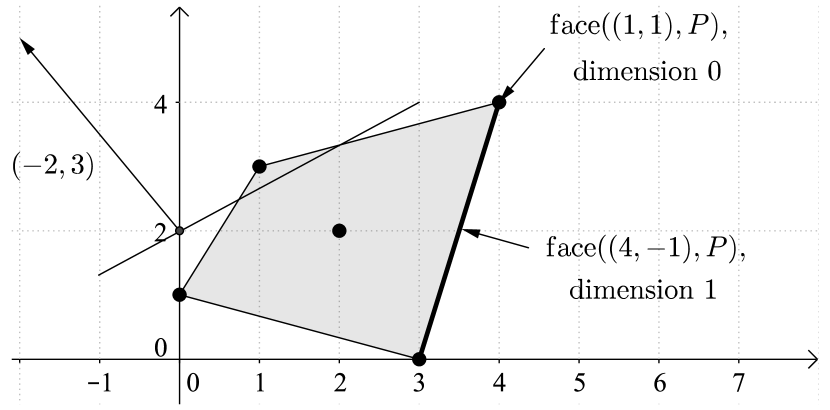
(a) The frame and the Newton polytope $P$ of $f$

0pt

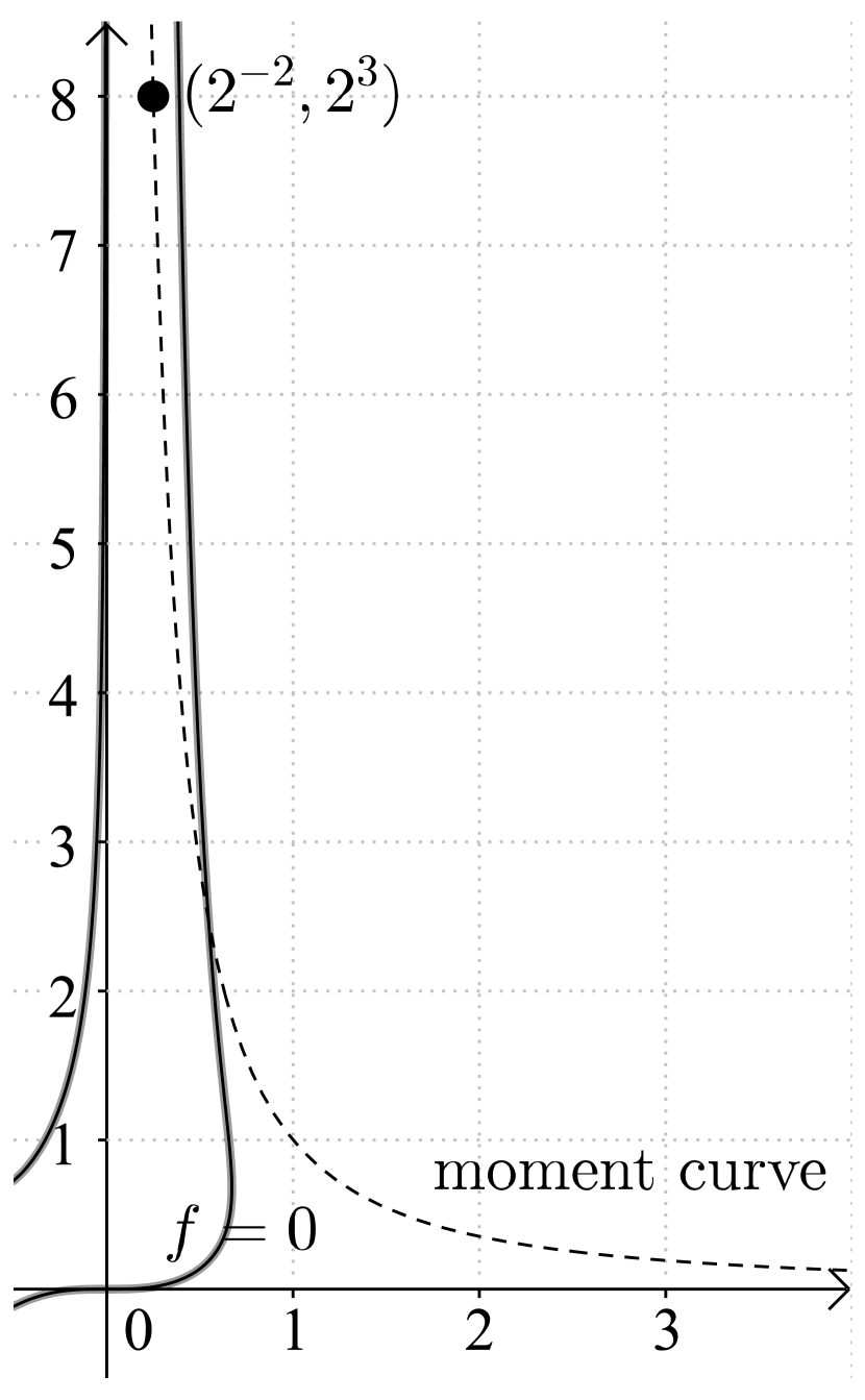
(b) The variety of $f$ and the moment curve $(a^{-2},a^{3})$

Figure 1: An illustration of Example 1, where $f=y+2xy^{3}-3x^{2}y^{2}-x^{3}-4x^{4}y^{4}$

The Newton polytope of a polynomial $f$ is the convex hull of its frame, $\operatorname{newton}(f)=\operatorname{conv}(\operatorname{frame}(f))$. Fig. 1(a) illustrates the Newton polytope of

$$y+2xy^{3}-3x^{2}y^{2}-x^{3}-4x^{4}y^{4}\in\mathbb{Z}[x,y],$$

which is the convex hull of its frame $\{(0,1),(1,3),(2,2),(3,0),(4,4)\}\subset\mathbb{N}^{2}$. As a convex hull of a finite set of points, the Newton polytope is bounded and thus indeed a polytope [26].

The face [26] of a polytope $P\subseteq\mathbb{R}^{d}$ with respect to a vector $\mathbf{n}\in\mathbb{R}^{d}$ is

$$\operatorname{face}(\mathbf{n},P)=\{\,\mathbf{p}\in P\mid\text{$\mathbf{n}^{T}\mathbf{p}\geq\mathbf{n}^{T}\mathbf{q}$ for all $\mathbf{q}\in P$}\,\}.$$

Faces of dimension $0$ are called vertices. We denote by $\operatorname{V}(P)$ the set of all vertices of $P$. We have $\mathbf{p}\in\operatorname{V}(P)$ if and only if there exists $\mathbf{n}\in\mathbb{R}^{d}$ such that $\mathbf{n}^{T}\mathbf{p}>\mathbf{n}^{T}\mathbf{q}$ for all $\mathbf{q}\in P\setminus\{\mathbf{p}\}$. In Fig.1(a), $(4,4)$ is a vertex of the Newton polytope with respect to $(1,1)$.

It is easy to see that for finite $S\subset\mathbb{R}^{d}$ we have

$$\operatorname{V}(\operatorname{conv}(S))\subseteq S\subseteq\operatorname{conv}(S).$$ (1)

The following lemma gives a characterization of $\operatorname{V}(\operatorname{conv}(S))$:

Lemma 1

Let $S\subset\mathbb{R}^{d}$ be finite, and let $\mathbf{p}\in S$. The following are equivalent:

1. $\mathbf{p}$ is a vertex of $\operatorname{conv}(S)$ with respect to $\mathbf{n}$.

2. There exists a hyperplane $H:\mathbf{n}^{T}\mathbf{x}+c=0$ that strictly separates $\mathbf{p}$ from $S\setminus\{\mathbf{p}\}$, and the normal vector $\mathbf{n}$ is directed from $H$ towards $\mathbf{p}$.

Proof

Assume (i). Then there exists $\mathbf{n}\in\mathbb{R}^{d}$ such that $\mathbf{n}^{T}\mathbf{p}>\mathbf{n}^{T}\mathbf{q}$ for all $\mathbf{q}\in S\setminus\{\mathbf{p}\}\subseteq\operatorname{conv}(S)\setminus\{\mathbf{p}\}$. Choose $\mathbf{q}_{0}\in S\setminus\{\mathbf{p}\}$ such that $\mathbf{n}^{T}\mathbf{q}_{0}$ is maximal, and choose $c$ such that $\mathbf{n}^{T}\mathbf{p}>-c>\mathbf{n}^{T}\mathbf{q}_{0}$. Then $\mathbf{n}^{T}\mathbf{p}+c>0$ and $\mathbf{n}^{T}\mathbf{q}+c\leq\mathbf{n}^{T}\mathbf{q}_{0}+c<0$ for all $\mathbf{q}\in S\setminus\{\mathbf{p}\}$. Hence $H:\mathbf{n}^{T}\mathbf{p}+c=0$ is the desired hyperplane.

Assume (ii). It follows that $\mathbf{n}^{T}\mathbf{p}+c>0>\mathbf{n}^{T}\mathbf{q}+c$ for all $\mathbf{q}\in S\setminus\{\mathbf{p}\}$. If $\mathbf{q}\in S\setminus\{\mathbf{p}\}$, then $\mathbf{n}^{T}\mathbf{p}>\mathbf{n}^{T}\mathbf{q}$. If, in contrast, $\mathbf{q}\in(\operatorname{conv}(S)\setminus S)\setminus\{\mathbf{p}\}=\operatorname{conv}(S)\setminus S$, then $\mathbf{q}=\sum_{\mathbf{s}\in S}t_{\mathbf{s}}\mathbf{s}$, where $t_{\mathbf{s}}\in[0,1]$, $\sum_{\mathbf{s}\in S}t_{\mathbf{s}}=1$, and at least two $t_{\mathbf{s}}$ are greater than $0$. It follows that

$$\mathbf{n}^{T}\mathbf{q}=\mathbf{n}^{T}\sum_{\mathbf{s}\in S}t_{\mathbf{s}}\mathbf{s}<\mathbf{n}^{T}\mathbf{p}\sum_{\mathbf{s}\in S}t_{\mathbf{s}}=\mathbf{n}^{T}\mathbf{p}.\quad\squareforqed$$

Let $S_{1}$, …, $S_{m}\subseteq\mathbb{R}^{d}$, and let $\mathbf{n}\in\mathbb{R}^{d}$. If there exist $\mathbf{p}_{1}\in S_{1}$, …, $\mathbf{p}_{n}\in S_{m}$ such that each $\mathbf{p}_{i}$ is a vertex of $\operatorname{conv}(S_{i})$ with respect to $\mathbf{n}$, then the (unique) vertex cluster of $\{S_{i}\}_{i\in\{1,\dots,m\}}$ with respect to $\mathbf{n}$ is defined as $(\mathbf{p}_{1},\dots,\mathbf{p}_{m})$.

3 Subtropical Real Root Finding Revisited

This section improves on the original method described in [27]. It furthermore lays some theoretical foundations to better understand the limitations of the heuristic approach. The method finds real zeros with all positive coordinates of a multivariate polynomial $f$ in three steps:

1. Evaluate $f(1,\dots,1)$. If this is $0$, we are done. If this is greater than $0$, then consider $-f$ instead of $f$. We may now assume that we have found $f(1,\dots,1)<0$.

2. Find $\mathbf{p}$ with all positive coordinates such that $f(\mathbf{p})>0$.

3. Use the Intermediate Value Theorem (a continuous function with positive and negative values has a zero) to construct a root of $f$ on the line segment $\overline{\mathbf{1}\mathbf{p}}$.

We focus here on Step 2. Our technique builds on [27, Lemma 4], which we are going to restate now in a slightly generalized form. While the original lemma required that $\mathbf{p}\in\operatorname{frame}(f)\setminus\{\mathbf{0}\}$, inspection of the proof shows that this limitation is not necessary:

Lemma 2

Let $f$ be a polynomial, and let $\mathbf{p}\in\operatorname{frame}(f)$ be a vertex of $\operatorname{newton}(f)$ with respect to $\mathbf{n}\in\mathbb{R}^{d}$. Then there exists $a_{0}\in\mathbb{R}^{+}$ such that for all $a\in\mathbb{R}^{+}$ with $a\geq a_{0}$ the following holds:

1. $\lvert f_{\mathbf{p}}\ a^{\mathbf{n}^{T}\mathbf{p}}\rvert>\lvert\sum_{\mathbf{q}\in\operatorname{frame}(f)\setminus\{\mathbf{p}\}}f_{\mathbf{q}}\ a^{\mathbf{n}^{T}\mathbf{q}}\rvert$,

2. $\operatorname{sign}(f(a^{\mathbf{n}}))=\operatorname{sign}(f_{\mathbf{p}})$.∎

In order to find a point with all positive coordinates where $f>0$, the original method iteratively examines each $\mathbf{p}\in\operatorname{frame}^{+}(f)\setminus\{\mathbf{0}\}$ to check if it is a vertex of $\operatorname{newton}(f)$ with respect to some $\mathbf{n}\in\mathbb{R}^{d}$. In the positive case, Lemma 2 guarantees for large enough $a\in\mathbb{R}^{+}$ that $\operatorname{sign}(f(a^{\mathbf{n}}))=\operatorname{sign}(f_{\mathbf{p}})=1$, in other words, $f(a^{\mathbf{n}})>0$.

Example 1

Consider $f=y+2xy^{3}-3x^{2}y^{2}-x^{3}-4x^{4}y^{4}$. Figure 1(a) illustrates the frame and the Newton polytope of $f$, of which $(1,3)$ is a vertex with respect to $(-2,3)$. Lemma 2 ensures that $f(a^{-2},a^{3})$ is strictly positive for sufficiently large positive $a$. For example, $f(2^{-2},2^{3})=\frac{51193}{256}$. Figure 1(b) shows how the moment curve $(a^{-2},a^{3})$ with $a\geq 2$ will not leave the sign invariant region of $f$ that contains $(2^{-2},2^{3})$.

An exponent vector $\mathbf{0}\in\operatorname{frame}(f)$ corresponds to an absolute summand $f_{\mathbf{0}}$ in $f$. Its above-mentioned explicit exclusion in [27, Lemma 4] originated from the false intuition that one cannot achieve $\operatorname{sign}(f(a^{\mathbf{n}}))=\operatorname{sign}(f_{\mathbf{0}})$ because the monomial $f_{\mathbf{0}}$ is invariant under the choice of $a$. However, inclusion of $\mathbf{0}$ can yield a normal vector $\mathbf{n}$ which renders all other monomials small enough for $f_{\mathbf{0}}$ to dominate.

Given a finite set $S\subset\mathbb{R}^{d}$ and a point $\mathbf{p}\in S$, the original method uses linear programming to determine if $\mathbf{p}$ is a vertex of $\operatorname{conv}(S)$ w.r.t. some vector $\mathbf{n}\in\mathbb{R}^{d}$. Indeed, from Lemma 1, the problem can be reduced to finding a hyperplane $H:\mathbf{n}^{T}\mathbf{x}+c=0$ that strictly separates $\mathbf{p}$ from $S\setminus\{\mathbf{p}\}$ with the normal vector $\mathbf{n}$ pointing from $H$ to $\mathbf{p}$. This is equivalent to solving the following linear problem with $d+1$ real variables $\mathbf{n}$ and $c$:

$$\varphi(\mathbf{p},S,\mathbf{n},c)\mathrel{\dot{=}}\mathbf{n}^{T}\mathbf{p}+c>0\land\bigwedge_{\mathbf{q}\in S\setminus\{\mathbf{p}\}}\mathbf{n}^{T}\mathbf{q}+c<0.$$ (2)

Notice that with the occurrence of a nonzero absolute summand the corresponding point $\mathbf{0}$ is generally a vertex of the Newton polytope with respect to $\mathbf{-1}=(-1,\dots,-1)$. This raises the question whether there are other special points that are certainly vertices of the Newton polytope. In fact, $\mathbf{0}$ is a lexicographic minimum in $\operatorname{frame}(f)$, and it is not hard to see that minima and maxima with respect to lexicographic orderings are generally vertices of the Newton polytope.

We are now going to generalize that observation. A monotonic total preorder ${\preceq}\subseteq\mathbb{Z}^{d}\times\mathbb{Z}^{d}$ is defined as follows:

1. $\mathbf{x}\preceq\mathbf{x}$ (reflexivity)

2. $\mathbf{x}\preceq\mathbf{y}\land\mathbf{y}\preceq\mathbf{z}\longrightarrow\mathbf{x}\preceq\mathbf{z}$ (transitivity)

3. $\mathbf{x}\preceq\mathbf{y}\longrightarrow\mathbf{x}+\mathbf{z}\preceq\mathbf{y}+\mathbf{z}$ (monotonicity)

4. $\mathbf{x}\preceq\mathbf{y}\lor\mathbf{y}\preceq\mathbf{x}$ (totality).

The difference to a total order is the missing anti-symmetry. As an example in $\mathbb{Z}^{2}$ consider $(x_{1},x_{2})\preceq(y_{1},y_{2})$ if and only if $x_{1}+x_{2}\leq y_{1}+y_{2}$. Then $-2\preceq 2$ and $2\preceq-2$ but $-2\neq 2$. Our definition of $\preceq$ on the extended domain $\mathbb{Z}^{d}$ guarantees a cancellation law $\mathbf{x}+\mathbf{z}\preceq\mathbf{y}+\mathbf{z}\longrightarrow\mathbf{x}\preceq\mathbf{y}$ also on $\mathbb{N}^{d}$. The following lemma follows by induction using monotonicity and cancellation:

Lemma 3

For $n\in\mathbb{N}\setminus\{0\}$ denote as usual the $n$-fold addition of $\mathbf{x}$ as $n\odot\mathbf{x}$. Then $\mathbf{x}\preceq\mathbf{y}\longleftrightarrow n\odot\mathbf{x}\preceq n\odot\mathbf{y}$.∎

Any monotonic preorder $\preceq$ on $\mathbb{Z}^{d}$ can be extended to $\mathbb{Q}^{d}$: Using a suitable principle denominator $n\in\mathbb{N}\setminus\{0\}$ define

$$\left(\frac{x_{1}}{n},\dots,\frac{x_{d}}{n}\right)\preceq\left(\frac{y_{1}}{n},\dots,\frac{y_{d}}{n}\right)\quad\text{if and only if}\quad(x_{1},\dots,x_{d})\preceq(y_{1},\dots,y_{d}).$$

This is well-defined.

Given $\mathbf{x}\preceq\mathbf{y}$ we have either $\mathbf{y}\npreceq\mathbf{x}$ or $\mathbf{y}\preceq\mathbf{x}$. In the former case we say that $\mathbf{x}$ and $\mathbf{y}$ are strictly preordered and write $\mathbf{x}\prec\mathbf{y}$. In the latter case they are not strictly preordered, i.e., $\mathbf{x}\nprec\mathbf{y}$ although we might have $\mathbf{x}\neq\mathbf{y}$. In particular, reflexivity yields $\mathbf{x}\preceq\mathbf{x}$ and hence certainly $\mathbf{x}\nprec\mathbf{x}$.

Example 2

Lexicographic orders are monotonic total orders and thus monotonic total preorders. Hence our notion covers our discussion of the absolute summand above. Here are some further examples: For $i\in\{1,\dots,d\}$ we define $\mathbf{x}\preceq_{i}\mathbf{y}$ if and only if $\pi_{i}(\mathbf{x})\leq\pi_{i}(\mathbf{y})$, where $\pi_{i}$ denotes the $i$-th projection. Similarly, $\mathbf{x}\succeq_{i}\mathbf{y}$ if and only if $\pi_{i}(\mathbf{x})\geq\pi_{i}(\mathbf{y})$. Next, $\mathbf{x}\preceq_{\Sigma}\mathbf{y}$ if and only if $\sum_{i}x_{i}\leq\sum_{i}y_{i}$. Our last example is going to be instrumental with the proof of the next theorem: Fix $\mathbf{n}\in\mathbb{R}^{d}$, and define for $\mathbf{p}$, $\mathbf{p}^{\prime}\in\mathbb{Z}^{d}$ that $\mathbf{p}\preceq_{\mathbf{n}}\mathbf{p^{\prime}}$ if and only if $\mathbf{n}^{T}\mathbf{p}\leq\mathbf{n}^{T}\mathbf{p^{\prime}}$.

Theorem 3.1

Let $f\in\mathbb{Z}[x_{1},\dots,x_{d}]$, and let $\mathbf{p}\in\operatorname{frame}(f)$. Then the following are equivalent:

1. $\mathbf{p}\in\operatorname{V}(\operatorname{newton}(f))$

2. There exists a monotonic total preorder $\preceq$ on $\mathbb{Z}^{d}$ such that

   $$\mathbf{p}=\max\nolimits_{\prec}(\operatorname{frame}(f)).$$

Proof

Let $\mathbf{p}$ be a vertex of $\operatorname{newton}(f)$ specifically with respect to $\mathbf{n}$. By our definition of a vertex in Sect. 2, $\mathbf{p}$ is the maximum of $\operatorname{frame}(f)$ with respect to $\prec_{\mathbf{n}}$.

Let, vice versa, $\preceq$ be a monotonic total preorder on $\mathbb{Z}^{d}$, and let $\mathbf{p}=\max_{\prec}(\operatorname{frame}(f))$. Shortly denote $V=\operatorname{V}(\operatorname{newton}(f))$, and assume for a contradiction that $\mathbf{p}\notin V$. Since $\mathbf{p}\in\operatorname{frame}(f)\subseteq\operatorname{newton}(f)$, we have

$$\mathbf{p}=\sum_{\mathbf{s}\in V}t_{\mathbf{s}}\mathbf{s},\quad\text{where}\quad t_{\mathbf{s}}\in[0,1]\quad\text{and}\quad\sum_{\mathbf{s}\in V}t_{\mathbf{s}}=1.$$

According to (1) in Sect. 2 we know that $V\subseteq\operatorname{frame}(f)\subseteq\operatorname{newton}(f)$. It follows that $\mathbf{s}\prec\mathbf{p}$ for all $\mathbf{s}\in V$, and using monotony we obtain

$$\mathbf{p}\prec\sum_{\mathbf{s}\in V}t_{\mathbf{s}}\mathbf{p}=\left(\sum_{\mathbf{s}\in V}t_{\mathbf{s}}\right)\mathbf{p}=\mathbf{p}.$$

On the other hand, we know that generally $\mathbf{p}\nprec\mathbf{p}$, a contradiction.∎

In Fig. 1(a) we have $(0,1)=\max_{\succeq_{1}}(\operatorname{frame}(f))$, $(3,0)=\max_{\succeq_{2}}(\operatorname{frame}(f))$, and $(4,4)=\max_{\preceq_{1}}(\operatorname{frame}(f))=\max_{\preceq_{2}}(\operatorname{frame}(f))$. This shows that, besides contributing to our theoretical understanding, the theorem can be used to substantiate the efficient treatment of certain special cases in combination with other methods for identifying vertices of the Newton polytope.

Corollary 1

Let $f\in\mathbb{Z}[x_{1},\dots,x_{d}]$, and let $\mathbf{p}\in\operatorname{frame}(f)$. If $p=\max(\operatorname{frame}(f))$ or $p=\min(\operatorname{frame}(f))$ with respect to an admissible term order in the sense of Gröbner Basis theory [7], then $p\in\operatorname{V}(\operatorname{newton}(f))$.∎

It is one of our research goals to identify and characterize those polynomials where the subtropical heuristic succeeds in finding positive points. We are now going to give a necessary criterion. Let $f\in\mathbb{Z}[x_{1},\dots,x_{d}]$, define ${\Pi(f)=\{\,\mathbf{r}\in\mathopen{]}0,\infty\mathclose{[}^{d}\mid f(\mathbf{r})>0\,\}}$, and denote by $\overline{\Pi(f)}$ its closure with respect to the natural topology. In Lemma 2, when $a$ tends to $\infty$, $a^{\mathbf{n}}$ will tend to some $\mathbf{r}\in\{0,\infty\}^{d}$. If $\mathbf{r}=\mathbf{0}$, then $\mathbf{0}\in\overline{\Pi(f)}$. Otherwise, $\Pi(f)$ is unbounded. Consequently, for the method to succeed, $\Pi$ must have at least one of those two properties. Figure 2 illustrates four scenarios: the subtropical method succeeds in the first three cases while it fails to find a point in $\Pi(f)$ in the last one. The first sub-figure presents a case where $\Pi(f)$ is unbounded. The second and third sub-figures illustrate cases where the closure of $\Pi(f)$ contains $(0,0)$. In the fourth sub-figure where neither $\Pi(f)$ is unbounded nor its closure contains $(0,0)$, the method cannot find any positive value of the variables for $f$ to be positive.

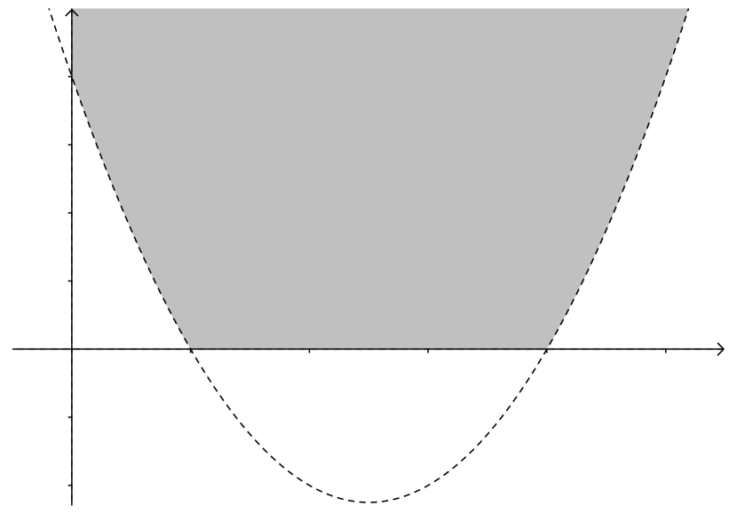
(a) $f=y-x^{2}+5x-4$

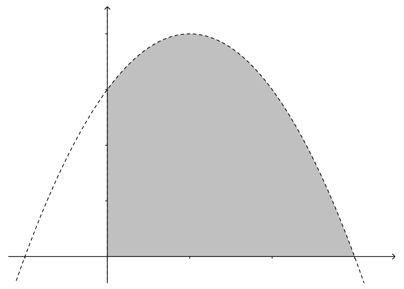
(b) $f=-y-x^{2}+2x+3$

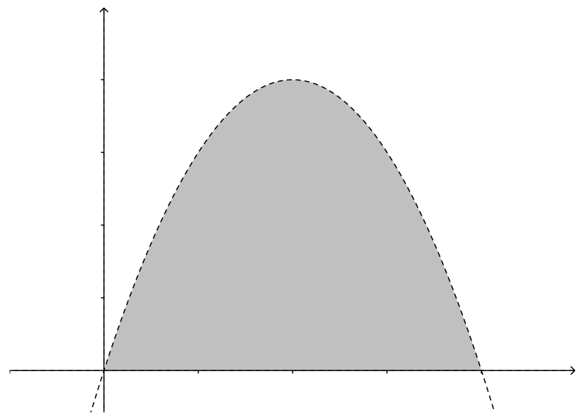
(c) $f=-y-x^{2}+4x$

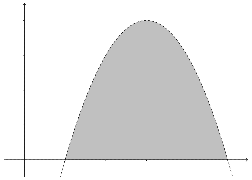
(d) $f=-y-x^{2}+6x-5$

Figure 2: Four scenarios of polynomials for the subtropical method. The shaded regions show $\Pi(f)$.

4 Positive Values of Several Polynomials

The subtropical method as presented in [27] finds zeros with all positive coordinates of one single multivariate polynomial. This requires to find a corresponding point with a positive value of the polynomial. In the sequel we restrict ourselves to this sub-task. This will allow us generalize from one polynomial to simultaneous positive values of finitely many polynomials.

4.1 A Sufficient Condition

With a single polynomial, the existence of a positive vertex of the Newton polytope guarantees the existence of positive real choices for the variables with a positive value of that polynomial. For several polynomials we introduce a more general notion: A sequence $(\mathbf{p}_{1},\dots,\mathbf{p}_{m})$ is a positive vertex cluster of $\{f_{i}\}_{i\in\{1,\dots,m\}}$ with respect to $\mathbf{n}\in\mathbb{R}^{d}$ if it is a vertex cluster of $\{\operatorname{frame}(f_{i})\}_{i\in\{1,\dots,m\}}$ with respect to $\mathbf{n}$ and $\mathbf{p}_{i}\in\operatorname{frame}^{+}(f_{i})$ for all $i\in\{1,\dots,m\}$. The existence of a positive vertex cluster will guarantee the existence of positive real choices of the variables such that all polynomials $f_{1}$, …, $f_{m}$ are simultaneously positive. The following lemma is a corresponding generalization of Lemma 2:

Lemma 4

If there exists a vertex cluster $(\mathbf{p}_{1},\dots,\mathbf{p}_{m})$ of $\{\operatorname{frame}(f_{i})\}_{i\in\{1,\dots,m\}}$ with respect to $\mathbf{n}\in\mathbb{R}^{n}$, then there exists $a_{0}\in\mathbb{R^{+}}$ such that the following holds for all $a\in\mathbb{R}^{+}$ with $a\geq a_{0}$ and all $i\in\{1,\dots,m\}$:

1. $\lvert(f_{i})_{\mathbf{p}_{i}}\ a^{\mathbf{n}^{T}\mathbf{p}_{i}}\rvert>\lvert\sum_{\mathbf{q}\in\operatorname{frame}(f_{i})\setminus\{\mathbf{p}_{i}\}}(f_{i})_{\mathbf{q}}\ a^{\mathbf{n}^{T}\mathbf{q}}\rvert$,

2. $\operatorname{sign}(f_{i}(a^{\mathbf{n}}))=\operatorname{sign}((f_{i})_{\mathbf{p}_{i}})$.

Proof

From [27, Lemma 4], for each $i\in\{1,\dots,m\}$, there exist $a_{0,i}\in\mathbb{R}^{+}$ such that for all $a\in\mathbb{R}^{+}$ with $a\geq a_{0,i}$ the following holds:

1. $\lvert(f_{i})_{\mathbf{p}_{i}}\ a^{\mathbf{n}^{T}\mathbf{p}_{i}}\rvert>\lvert\sum_{\mathbf{q}\in\operatorname{frame}(f_{i})\setminus\{\mathbf{p}_{i}\}}(f_{i})_{\mathbf{q}}\ a^{\mathbf{n}^{T}\mathbf{q}}\rvert$,

2. $\operatorname{sign}(f_{i}(a^{n}))=\operatorname{sign}((f_{i})_{\mathbf{p}_{i}})$.

It now suffices to take $a_{0}=\max\{a_{0,i}\ |\ 1\leq i\leq m\}$. ∎

Similarly to the case of one polynomial, the following Proposition provides a sufficient condition for the existence of a common point with positive value for multiple polynomials.

Proposition 1

If there exists a positive vertex cluster $(\mathbf{p}_{1},\dots,\mathbf{p}_{m})$ of the polynomials $\{f_{i}\}_{i\in\{1,\dots,m\}}$ with respect to a vector $\mathbf{n}\in\mathbb{R}^{d}$, then there exists $a_{0}\in\mathbb{R}^{+}$ such that for all $a\in\mathbb{R}^{+}$ with $a\geq a_{0}$ the following holds:

$$\bigwedge_{i=1}^{m}f_{i}(a^{\mathbf{n}})>0.$$

Proof

For $i\in\{1,\dots,m\}$, since $\mathbf{p}_{i}\in\operatorname{frame}^{+}(f_{i})$, Lemma 4 implies $f_{i}(a^{\mathbf{n}})>0$.∎

Example 3

Consider $f_{1}=2-xy^{2}z+x^{2}yz^{3},f_{2}=3-xy^{2}z^{4}-x^{2}z-x^{4}y^{3}z^{3},$ and $f_{3}=4-z-y-x+4$. The exponent vector $\mathbf{0}$ is a vertex of $\text{newton}(f_{1})$, $\operatorname{newton}(f_{2})$, and $\operatorname{newton}(f_{3})$ with respect to $(-1,-1,-1)$. Choose $a_{0}=2\in\mathbb{R}^{+}$. Then for all $a\in\mathbb{R}$ with $a\geq a_{0}$ we have $f_{1}(a^{-1},a^{-1},a^{-1})>0\land f_{2}(a^{-1},a^{-1},a^{-1})>0\land f_{3}(a^{-1},a^{-1},a^{-1})>0$. ∎

4.2 Existence of Positive Vertex Clusters

Given polynomials $f_{1}$, …, $f_{m}$, Proposition 1 provides a sufficient condition, i.e. the existence of a positive vertex cluster of $\{f_{i}\}_{i\in\{1,\dots,m\}}$, for the satisfiability of $\bigwedge_{i=1}^{m}f_{i}>0$. A straightforward method to decide the existence of such a cluster is to verify whether each $(\mathbf{p}_{1},\dots,\mathbf{p}_{m})\in\operatorname{frame}^{+}(f_{1})\times\cdots\times\operatorname{frame}^{+}(f_{m})$ is a positive vertex cluster by checking the satisfiability of the formula

$$\bigwedge\limits_{i\in\{1,\dots,m\}}\varphi(\mathbf{p}_{i},\operatorname{frame}(f_{i}),\mathbf{n},c_{i}),$$

where $\varphi$ is defined as in (2) on p.2. This is a linear problem with $d+m$ variables $\mathbf{n}$, $c_{1}$, …, $c_{m}$. Since $\operatorname{frame}(f_{1})$, …, $\operatorname{frame}(f_{m})$ are finite, checking all $m$-tuples $(\mathbf{p}_{1},\dots,\mathbf{p}_{m})$ will terminate, provided we rely on a complete algorithm for linear programming, such as the Simplex algorithm [10], the ellipsoid method [22], or the interior point method [21]. This provides a decision procedure for the existence of a positive vertex cluster of $\{f_{i}\}_{i\in\{1,\dots,m\}}$. However, this requires checking all candidates in $\operatorname{frame}^{+}(f_{1})\times\cdots\times\operatorname{frame}^{+}(f_{m})$.

We propose to use instead state-of-the-art SMT solving techniques over linear real arithmetic to examine whether or not $\{f_{i}\}_{i\in\{1,\dots,m\}}$ has a positive vertex cluster with respect to some $\mathbf{n}\in\mathbb{R}^{d}$. In the positive case, a solution for $\bigwedge_{i=1}^{m}f_{i}>0$ can be constructed as $a^{\mathbf{n}}$ with a sufficiently large $a\in\mathbb{R}^{+}$.

To start with, we provide a characterization for the positive frame of a single polynomial to contain a vertex of the Newton polytope.

Lemma 5

Let $f\in\mathbb{Z}[\mathbf{x}]$. The following are equivalent:

1. There exists a vertex $\mathbf{p}\in\operatorname{frame}^{+}(f)$ of $\operatorname{newton}(f)=\operatorname{conv}(\operatorname{frame}(f))$ with respect to $\mathbf{n}\in\mathbb{R}^{d}$.

2. There exists a vertex $\mathbf{p}^{\prime}\in\operatorname{frame}^{+}(f)$ such that $\mathbf{p}^{\prime}$ is also a vertex of ${\operatorname{conv}(\operatorname{frame}^{-}(f)\cup\{\mathbf{p}^{\prime}\})}$ with respect to $\mathbf{n^{\prime}}\in\mathbb{R}^{d}$.

Proof

Assume (i). Take $\mathbf{p}^{\prime}=\mathbf{p}$ and $\mathbf{n}^{\prime}=\mathbf{n}$. Since $\mathbf{p}$ is a vertex of $\text{newton}(f)$ with respect to $\mathbf{n}$, $\mathbf{n}^{T}\mathbf{p}>\mathbf{n}^{T}\mathbf{p}_{1}$ for all $\mathbf{p}_{1}\in\operatorname{frame}(f)\setminus\{\mathbf{p}\}$. This implies that $\mathbf{n}^{T}\mathbf{p}>\mathbf{n}^{T}\mathbf{p}_{1}$ for all $\mathbf{p}_{1}\in\operatorname{frame}^{-}(f)\setminus\{\mathbf{p}\}=\left(\operatorname{frame}^{-}(f)\cup\{\mathbf{p}\}\right)\setminus\{\mathbf{p}\}$. In other words, $\mathbf{p}$ is a vertex of $\operatorname{conv}(\operatorname{frame}^{-}(f)\cup\{\mathbf{p}\})$ with respect to $\mathbf{n}$.

Assume (ii). Suppose $V=\operatorname{V}(\operatorname{newton}(f))\subseteq\operatorname{frame}^{-}(f)$. Then, $\mathbf{p}^{\prime}=\sum_{\mathbf{s}\in V}t_{\mathbf{s}}\mathbf{s}$ where $t_{\mathbf{s}}\in[0,1]$, $\sum_{\mathbf{s}\in V}t_{\mathbf{s}}=1$. It follows that

$$\mathbf{n}^{\prime T}\mathbf{p}^{\prime}=\sum_{\mathbf{s}\in V}t_{\mathbf{s}}\mathbf{n}^{\prime T}\mathbf{s}<\sum_{\mathbf{s}\in V}t_{\mathbf{s}}\mathbf{n}^{\prime T}\mathbf{p}^{\prime}=\mathbf{n}^{\prime T}\mathbf{p}^{\prime}\sum_{\mathbf{s}\in V}t_{\mathbf{s}}=\mathbf{n}^{\prime T}\mathbf{p}^{\prime},$$

which is a contradiction. As a result, there must be some $\mathbf{p}\in\operatorname{frame}^{+}(f)$ which is a vertex of $\operatorname{newton}(f)$ with respect to some $\mathbf{n}\in\mathbb{R}^{d}$. ∎

Thus some $\mathbf{p}\in\operatorname{frame}^{+}(f)$ is a vertex of the Newton polytope of a polynomial $f$ if and only if the following formula is satisfiable:

$$\psi(f,\mathbf{n^{\prime}},c) \mathrel{\dot{=}}\bigvee_{\mathbf{p}\in\operatorname{frame}^{+}(f)}\varphi\left(\mathbf{p},\operatorname{frame}^{-}(f)\cup\{\mathbf{p}\},\mathbf{n^{\prime}},c\right)$$

$$\equiv\bigvee_{\mathbf{p}\in\operatorname{frame}^{+}(f)}\left[\mathbf{n^{\prime}}^{T}\mathbf{p}+c>0\land\bigwedge_{\mathbf{q}\in\operatorname{frame}^{-}(f)}\mathbf{n^{\prime}}^{T}\mathbf{q}+c<0\right]$$

$$\equiv\left[\bigvee_{\mathbf{p}\in\operatorname{frame}^{+}(f)}\mathbf{n^{\prime}}^{T}\mathbf{p}+c>0\right]\land\left[\bigwedge_{\mathbf{p}\in\operatorname{frame}^{-}(f)}\mathbf{n^{\prime}}^{T}\mathbf{p}+c<0\right].$$

For the case of several polynomials, the following theorem is a direct consequence of Lemma 5.

Theorem 4.1

Polynomials $\{f_{i}\}_{i\in\{1,\dots,m\}}$ have a positive vertex cluster with respect to $\mathbf{n}\in\mathbb{R}^{d}$ if and only if $\bigwedge_{i=1}^{m}\psi(f_{i},\mathbf{n},c_{i})$ is satisfiable. ∎

The formula $\bigwedge_{i=1}^{m}\psi(f_{i},\mathbf{n},c_{i})$ can be checked for satisfiability using combinations of linear programming techniques and DPLL($T$) procedures [11, 16], i.e., satisfiability modulo linear arithmetic on reals. Any SMT solver supporting the QF_LRA logic is suitable. In the satisfiable case $\{f_{i}\}_{i\in\{1,\dots,m\}}$ has a positive vertex cluster and we can construct a solution for $\bigwedge_{i=1}^{m}f_{i}>0$ as discussed earlier.

Example 4

Consider $f_{1}=-12+2x^{12}y^{25}z^{49}-31x^{13}y^{22}z^{110}-11x^{1000}y^{500}z^{89}$ and $f_{2}=-23+5xy^{22}z^{110}-21x^{15}y^{20}z^{1000}+2x^{100}y^{2}z^{49}$. With $\mathbf{n}=(n_{1},n_{2},n_{3})$ this yields

$$\psi(f_{1},\mathbf{n},c_{1}) =12n_{1}+25n_{2}+49n_{3}+c_{1}>0\land 13n_{1}+22n_{2}+110n_{3}+c_{1}<0$$

$$\land 1000n_{1}+500n_{2}+89n_{3}+c_{1}<0\land c_{1}<0,$$

$$\psi(f_{2},\mathbf{n},c_{2}) =(n_{1}+22n_{2}+110n_{3}+c_{2}>0\lor 100n_{1}+2n_{2}+49n_{3}+c_{2}>0)$$

$$\land 15n_{1}+20n_{2}+1000n_{3}+c_{2}<0\land c_{2}<0.$$

The conjunction $\psi(f_{1},\mathbf{n},c_{1})\land\psi(f_{2},\mathbf{n},c_{2})$ is satisfiable. The SMT solver CVC4 computes $\mathbf{n}=(-\frac{238834}{120461},\frac{2672460}{1325071},-\frac{368561}{1325071})$ and $c_{1}=c_{2}=-1$ as a model. Theorem 4.1 and Proposition 1 guarantee that there exists a large enough $a\in\mathbb{R}^{+}$ such that $f_{1}(a^{\mathbf{n}})>0\land f_{2}(a^{\mathbf{n}})>0$. Indeed, $a=2$ already yields $f_{1}(a^{\mathbf{n}})\approx 16371.99$ and $f_{2}(a^{\mathbf{n}})\approx 17707.27$. ∎

5 More General Solutions

So far all variables were assumed to be strictly positive, i.e., only solutions $\mathbf{x}\in\mathopen{]}0,\infty\mathclose{[}^{d}$ were considered. This section proposes a method for searching over $\mathbb{R}^{d}$ by encoding sign conditions along with the condition in Theorem 4.1 as a quantifier-free formula over linear real arithmetic.

Let $V=\{x_{1},\dots,x_{d}\}$ be the set of variables. We define a sign variant of $V$ as a function $\tau:V\mapsto V\cup\{-x\mid x\in V\}$ such that for each $x\in V$, $\tau(x)\in\{x,-x\}$. We write $\tau(f)$ to denote the substitution $f(\tau(x_{1}),\dots,\tau(x_{d}))$ of $\tau$ into a polynomial $f$. Furthermore, $\tau(a)$ denotes $\bigl{(}\frac{\tau(x_{1})}{x_{1}}a,\dots,\frac{\tau(x_{d})}{x_{d}}a\bigr{)}$ for $a\in\mathbb{R}$. A sequence $(\mathbf{p}_{1},\dots,\mathbf{p}_{m})$ is a variant positive vertex cluster of $\{f_{i}\}_{i\in\{1,\dots,m\}}$ with respect to a vector $\mathbf{n}\in\mathbb{R}^{d}$ and a sign variant $\tau$ if $(\mathbf{p}_{1},\dots,\mathbf{p}_{m})$ is a positive vertex cluster of $\{\tau(f_{i})\}_{i\in\{1,\dots,m\}}$. Note that the substitution of $\tau$ into a polynomial $f$ does not change the exponent vectors in $f$ in terms of their exponents values, but only possibly changes signs of monomials. Given $\mathbf{p}=(p_{1},\dots,p_{d})\in\mathbb{N}^{d}$ and a sign variant $\tau$, we define a formula $\vartheta(\mathbf{p},\tau)$ such that it is true if and only if the sign of the monomial associated with $\mathbf{p}$ is changed after applying the substitution defined by $\tau$:

$$\vartheta(\mathbf{p},\tau)\mathrel{\dot{=}}\bigoplus\limits_{i=1}^{d}\bigl{(}\tau(x_{i})=-x_{i}\land(p_{i}\bmod 2=1)\bigr{)}.$$

Note that this xor expression becomes true if and only if an odd number of its operands are true. Furthermore, a variable can change the sign of a monomial only when its exponent in that monomial is odd. As a result, if $\vartheta(\mathbf{p},\tau)$ is true, then applying the substitution defined by $\tau$ will change the sign of the monomial associated with $\mathbf{p}$. In conclusion, some $\mathbf{p}\in\operatorname{frame}(f)$ is in the positive frame of $\tau(f)$ if and only if one of the following mutually exclusive conditions holds:

1. $\mathbf{p}\in\operatorname{frame}^{+}(f)$ and $\vartheta(\mathbf{p},\tau)=\textsc{false}$

2. $\mathbf{p}\in\operatorname{frame}^{-}(f)$ and $\vartheta(\mathbf{p},\tau)=\textsc{true}$.

In other words, $\mathbf{p}$ is in the positive frame of $\tau(f)$ if and only if the formula $\Theta(\mathbf{p},f,\tau)\mathrel{\dot{=}}\big{(}f_{\mathbf{p}}>0\land\neg\vartheta(\mathbf{p},\tau)\big{)}\lor\big{(}f_{\mathbf{p}}<0\land\vartheta(\mathbf{p},\tau)\big{)}$ holds. Then, the positive and negative frames of $\tau(f)$ parameterized by $\tau$ are defined as

$$\operatorname{frame}^{+}(\tau(f)) = \{\,\mathbf{p}\in\operatorname{frame}(f)\mid\Theta(\mathbf{p},f,\tau)\,\},$$

$$\operatorname{frame}^{-}(\tau(f)) = \{\,\mathbf{p}\in\operatorname{frame}(f)\mid\neg\Theta(\mathbf{p},f,\tau)\,\},$$

respectively. The next lemma provides a sufficient condition for the existence of a solution in $\mathbb{R}^{d}$ of $\bigwedge_{i=1}^{m}f_{i}>0$.

Lemma 6

If there exists a variant positive vertex cluster of $\{f_{i}\}_{i\in\{1,\dots,m\}}$ with respect to $\mathbf{n}\in\mathbb{R}^{d}$ and a sign variant $\tau$, then there exists $a_{0}\in\mathbb{R}^{+}$ such that for all $a\in\mathbb{R}^{+}$ with $a\geq a_{0}$ the following holds:

$$\bigwedge_{i=1}^{m}f_{i}\big{(}\tau(a)^{\mathbf{n}}\big{)}>0.$$

Proof

Since $\{\tau(f_{i})\}_{i\in\{1,\dots,m\}}$ has a positive vertex cluster with respect to $\mathbf{n}$, Proposition 1 guarantees that there exists $a_{0}\in\mathbb{R}$ such that for all $a\in\mathbb{R}$ with $a\geq a_{0}$, we have $\bigwedge_{i=1}^{m}\tau(f_{i})(a^{\mathbf{n}})>0$, or $\bigwedge_{i=1}^{m}f_{i}\big{(}\tau(a)^{\mathbf{n}}\big{)}>0$. ∎

A variant positive vertex cluster exists if and only if there exist $\mathbf{n}\in\mathbb{R}^{d}$, $c_{1},\dots,c_{m}\in\mathbb{R}$, and a sign variant $\tau$ such that the following formula becomes true:

$$\Psi(f_{1},\dots,f_{m},\mathbf{n},c_{1},\dots,c_{m},\tau)\mathrel{\dot{=}}\bigwedge_{i=1}^{m}\psi\big{(}\tau(f_{i}),\mathbf{n},c_{i}\big{)},$$

where for $i\in\{1,\dots,m\}$:

$$\psi\big{(}\tau(f_{i}),\mathbf{n},c_{i}\big{)} \equiv \left[\bigvee_{\mathbf{p}\in\operatorname{frame}^{+}(\tau(f_{i}))}\mathbf{n}^{T}\mathbf{p}+c_{i}>0\right]\land\left[\bigwedge_{\mathbf{p}\in\operatorname{frame}^{-}(\tau(f_{i}))}\mathbf{n}^{T}\mathbf{p}+c_{i}<0\right]$$

$$\equiv \phantom{\land\ }\left[\bigvee_{\mathbf{p}\in\operatorname{frame}(f_{i})}\Theta(\mathbf{p},f_{i},\tau)\land\mathbf{n}^{T}\mathbf{p}+c_{i}>0\right]$$

$$\land\ \left[\bigwedge_{\mathbf{p}\in\operatorname{frame}(f_{i})}\Theta(\mathbf{p},f_{i},\tau)\lor\mathbf{n}^{T}\mathbf{p}+c_{i}<0\right].$$

The sign variant $\tau$ can be encoded as $d$ Boolean variables $b_{1}$, …, $b_{d}$ such that $b_{i}$ is true if and only if $\tau(x_{i})=-x_{i}$ for all $i\in\{1,\dots,d\}$. Then, the formula $\Psi(f_{1},\dots,f_{m},\mathbf{n},c_{1},\dots,c_{m},\tau)$ can be checked for satisfiability using an SMT solver for quantifier-free logic with linear real arithmetic.

6 Application to SMT Benchmarks

A library STROPSAT implementing Subtropical Satisfiability, is available on our web page. It is integrated into veriT [6] as an incomplete theory solver for non-linear arithmetic benchmarks. We experimented on the QF_NRA category of the SMT-LIB on all benchmarks consisting of only inequalities, that is $4917$ formulas out of $11601$ in the whole category. The experiments thus focus on those $4917$ benchmarks, comprising $3265$ sat-annotated ones, $106$ unknowns, and $1546$ unsat benchmarks. We used the SMT solver CVC4 to handle the generated linear real arithmetic formulas $\Psi(f_{1},\dots,f_{m},\mathbf{n},c_{1},\dots,c_{m},\tau)$, and we ran veriT (with STROPSAT as the theory solver) against the clear winner of the SMT-COMP 2016 on the QF_NRA category, i.e., Z3 (implementing nlsat [20]), on a CX250 Cluster with Intel Xeon E5-2680v2 2.80GHz CPUs. Each pair of benchmark and solver was run on one CPU with a timeout of 2500 seconds and 20 GB memory. The experimental data and the library are also available on Zenodo.

Since our method focuses on showing satisfiability, only brief statistics on unsat benchmarks are provided. Among the $1546$ unsat benchmarks, 200 benchmarks are found unsatisfiable already by the linear arithmetic theory reasoning in veriT. For each of the remaining ones, the method quickly returns unknown within 0.002 to 0.096 seconds, with a total cumulative time of 18.45 seconds (0.014 seconds on average). This clearly shows that the method can be applied with a very small overhead, upfront of another, complete or less incomplete procedure to check for unsatisfiability.

Table 1 provides the experimental results on benchmarks with sat or unknown status, and the cumulative times. The meti-tarski family consists of small benchmarks (most of them contain 3 to 4 variables and 1 to 23 polynomials with degrees between 1 and 4). Those are proof obligations extracted from the MetiTarski project [1], where the polynomials represent approximations of elementary real functions; all of them have defined statuses. The zankl family consists of large benchmarks (large numbers of variables and polynomials but small degrees) stemming from termination proofs for term-rewriting systems [14].

Table 1: Comparison between STROPSAT and Z3 (times in seconds)

Family	STROPSAT				Z3
	sat	Time	unkown	Time	sat	Time	unsat	Time
meti-tarski (sat - 3220)	2359	32.37	861	10.22	3220	88.55	0	0
zankl (sat - 45)	29	3.77	16	0.59	42	2974.35	0	0
zankl (unknown - 106)	15	2859.44	76	6291.33	14	1713.16	23	1.06

Although Z3 clearly outperforms STROPSAT in the number of solved benchmarks, the results also clearly show that our method is a useful complementing heuristic with little drawback, to be used either upfront or in portfolio with other approaches. As already said, it returns unknown quickly on unsat benchmarks. In particular, on all benchmarks solved by Z3 only, STROPSAT returns unknown quickly (see Fig. 4).

When both solvers can solve the same benchmark, the running time of STROPSAT is comparable with Z3 (Fig. 3). There are $11$ large benchmarks ($9$ of them have the unknown status) that are solved by STROPSAT but time out with Z3. STROPSAT times out for only $15$ problems, on which Z3 times out as well. STROPSAT provides a model for $15$ unknown benchmarks, whereas Z3 times out on 9 of them. The virtual best solver (i.e. running Z3 and STROPSAT in parallel and using the quickest answer) decreases the execution time for the meti-tarski problems to 54.43 seconds, solves all satisfiable zankl problems in 1120 seconds, and 24 of the unknown ones in 4502 seconds.

Since the exponents of the polynomials become coefficients in the linear formulas, high degrees do not hurt our method significantly. As the SMT-LIB does not currently contain any inequality benchmarks with high degrees, our experimental results above do not demonstrate this claim. However, formulas like in Example 4 are totally within reach of our method (STROPSAT returned sat within a second) while Z3 runs out of memory ($20$ GB) after 30 seconds for the constraint $f_{1}>0\land f_{2}>0$.

Figure 3: STROPSAT returns sat or timeout ($2418$ benchmarks, times in seconds)

Figure 4: STROPSAT returns unknown ($2299$ benchmarks, times in seconds)

7 Conclusion

We presented some extensions of a heuristic method to find simultaneous positive values of nonlinear multivariate polynomials. Our techniques turn out useful to handle SMT problems. In practice, our method is fast, either to succeed or to fail, and it succeeds where state-of-the-art solvers do not. Therefore it establishes a valuable heuristic to apply either before or in parallel with other more complete methods to deal with non-linear constraints. Since the heuristic translates a conjunction of non-linear constraints one to one into a conjunction of linear constraints, it can easily be made incremental by using an incremental linear solver.

To improve the completeness of the method, it could be helpful to not only consider vertices of Newton polytopes, but also faces. Then, the value of the coefficients and not only their sign would matter. Consider $\{\mathbf{p}_{1},\mathbf{p}_{2},\mathbf{p}_{3}\}=\operatorname{face}(\mathbf{n},\operatorname{newton}(f))$, then we have $\mathbf{n}^{T}\mathbf{p}_{1}=\mathbf{n}^{T}\mathbf{p}_{2}=\mathbf{n}^{T}\mathbf{p}_{3}$. It is easy to see that $f_{\mathbf{p}_{1}}\mathbf{x}^{\mathbf{p}_{1}}+f_{\mathbf{p}_{2}}\mathbf{x}^{\mathbf{p}_{2}}+f_{\mathbf{p}_{3}}\mathbf{x}^{\mathbf{p}_{3}}$ will dominate the other monomials in the direction of $\mathbf{n}$. In other words, there exists $a_{0}\in\mathbb{R}$ such that for all $a\in\mathbb{R}$ with $a\geq a_{0}$, $\operatorname{sign}(f(a^{\mathbf{n}}))=\operatorname{sign}(f_{\mathbf{p}_{1}}+f_{\mathbf{p}_{2}}+f_{\mathbf{p}_{3}})$. We leave for future work the encoding of the condition for the existence of such a face into linear formulas.

In the last paragraph of Section 3, we showed that, for the subtropical method to succeed, the set of values for which the considered polynomial is positive should either be unbounded, or should contain points arbitrarily near $\mathbf{0}$. We believe there is a stronger, sufficient condition, that would bring another insight to the subtropical method.

We leave for further work two interesting questions suggested by a reviewer, both concerning the case when the method is not able to assert the satisfiability of a set of literals. First, the technique could indeed be used to select, using the convex hull of the frame, some constraints most likely to be part of an unsatisfiable set; this could be used to simplify the work of the decision procedure to check unsatisfiability afterwards. Second, a careful analysis of the frame can provide information to remove some constraints in order to have a provable satisfiable set of constraints; this could be of some use for in a context of max-SMT.

Finally, on a more practical side, we would like to investigate the use of the techniques presented here for the testing phase of the raSAT loop [28], an extension the interval constraint propagation with testing and the Intermediate Value Theorem. We believe that this could lead to significant improvements in the solver, where testing is currently random.

References

- [1] Akbarpour, B., Paulson, L.C.: MetiTarski: An automatic theorem prover for real-valued special functions. Journal of Automated Reasoning 44(3) (2010) 175–205
- [2] Barrett, C., Kroening, D., Melham, T.: Problem solving for the 21st century: Efficient solvers for satisfiability modulo theories. Technical Report 3, London Mathematical Society and Smith Institute for Industrial Mathematics and System Engineering (2014) Knowledge Transfer Report.
- [3] Barrett, C., Sebastiani, R., Seshia, S.A., Tinelli, C.: Satisfiability modulo theories. In: Handbook of Satisfiability. Volume 185 of Frontiers in Artificial Intelligence and Applications. IOS Press (2009) 825–885
- [4] Benhamou, F., Granvilliers, L.: Continuous and interval constraints. In: Handbook of Constraint Programming. Elsevier, New York (2006) 571–604
- [5] Bofill, M., Nieuwenhuis, R., Oliveras, A., Rodríguez-Carbonell, E., Rubio, A.: The Barcelogic SMT solver. In: Computer Aided Verification. Springer (2008) 294–298
- [6] Bouton, T., Caminha B. De Oliveira, D., Déharbe, D., Fontaine, P.: veriT: An open, trustable and efficient SMT-Solver. In: Proceedings of the 22nd International Conference on Automated Deduction. CADE-22, Springer (2009) 151–156
- [7] Buchberger, B.: Ein Algorithmus zum Auffinden der Basiselemente des Restklassenringes nach einem nulldimensionalen Polynomideal. Doctoral dissertation, University of Innsbruck, Austria (1965)
- [8] Cimatti, A., Griggio, A., Irfan, A., Roveri, M., Sebastiani, R.: Invariant checking of NRA transition systems via incremental reduction to LRA with EUF. In: Tools and Algorithms for the Construction and Analysis of Systems: 23rd International Conference, TACAS 2017. Springer (2017) 58–75
- [9] Corzilius, F., Loup, U., Junges, S., Ábrahám, E.: SMT-RAT: An SMT-compliant nonlinear real arithmetic toolbox. In: Theory and Applications of Satisfiability Testing – SAT 2012. Springer (2012) 442–448
- [10] Dantzig, G.B.: Linear programming and extensions. Prentice University Press, Princeton, NJ (1963)
- [11] Dutertre, B., de Moura, L.: A fast linear-arithmetic solver for DPLL(T). In: Computer Aided Verification. Springer (2006) 81–94
- [12] Errami, H., Eiswirth, M., Grigoriev, D., Seiler, W.M., Sturm, T., Weber, A.: Detection of Hopf bifurcations in chemical reaction networks using convex coordinates. Journal of Computational Physics 291 (2015) 279–302
- [13] Fränzle, M., Herde, C., Teige, T., Ratschan, S., Schubert, T.: Efficient solving of large non-linear arithmetic constraint systems with complex Boolean structure. Journal on Satisfiability, Boolean Modeling and Computation 1 (2007) 209–236
- [14] Fuhs, C., Giesl, J., Middeldorp, A., Schneider-Kamp, P., Thiemann, R., Zankl, H.: SAT solving for termination analysis with polynomial interpretations. In: Theory and Applications of Satisfiability Testing – SAT 2007. Springer (2007) 340–354
- [15] Ganai, M., Ivancic, F.: Efficient decision procedure for non-linear arithmetic constraints using CORDIC. In: Formal Methods in Computer-Aided Design, 2009. FMCAD 2009. (2009) 61–68
- [16] Ganzinger, H., Hagen, G., Nieuwenhuis, R., Oliveras, A., Tinelli, C.: DPLL(T): Fast decision procedures. In: Computer Aided Verification. Springer (2004) 175–188
- [17] Gao, S., Kong, S., Clarke, E.M.: Satisfiability modulo ODEs. In: Formal Methods in Computer-Aided Design (FMCAD), 2013. (2013) 105–112
- [18] Gao, S., Kong, S., Clarke, E.: dReal: An SMT solver for nonlinear theories over the reals. In: Automated Deduction – CADE-24. Springer (2013) 208–214
- [19] Granvilliers, L., Benhamou, F.: RealPaver: An interval solver using constraint satisfaction techniques. ACM Transactions on Mathematical Software 32 (2006) 138–156
- [20] Jovanović, D., de Moura, L.: Solving non-linear arithmetic. In: Automated Reasoning. Springer (2012) 339–354
- [21] Karmarkar, N.: A new polynomial-time algorithm for linear programming. Combinatorica 4(4) (1984) 373–395
- [22] Khachiyan, L.: Polynomial algorithms in linear programming. USSR Computational Mathematics and Mathematical Physics 20(1) (1980) 53–72
- [23] Passmore, G.O.: Combined decision procedures for nonlinear arithmetics, real and complex. Dissertation, School of Informatics, University of Edinburgh (2011)
- [24] Passmore, G.O., Jackson, P.B.: Combined decision techniques for the existential theory of the reals. In: Intelligent Computer Mathematics, Springer (2009) 122–137
- [25] Ratschan, S.: Efficient solving of quantified inequality constraints over the real numbers. ACM Transactions on Computational Logic 7 (2006) 723–748
- [26] Schrijver, A.: Theory of Linear and Integer Programming. John Wiley & Sons, Inc., New York, NY (1986)
- [27] Sturm, T.: Subtropical real root finding. In: Proceedings of the ISSAC 2015. ACM (2015) 347–354
- [28] Vu, X.T., Van Khanh, T., Ogawa, M.: raSAT: An SMT solver for polynomial constraints. In: Automated Reasoning. Springer (2016) 228–237
- [29] Zankl, H., Middeldorp, A.: Satisfiability of non-linear (ir)rational arithmetic. In: Logic for Programming, Artificial Intelligence, and Reasoning. Springer (2010) 481–500