Abstract

The last decades have seen an unprecedented increase in the availability of data sets that are inherently global and temporally evolving, from remotely sensed networks to climate model ensembles. This paper provides a view of statistical modeling techniques for space-time processes, where space is the sphere representing our planet. In particular, we make a distintion between (a) second order-based, and (b) practical approaches to model temporally evolving global processes. The former are based on the specification of a class of space-time covariance functions, with space being the two-dimensional sphere. The latter are based on explicit description of the dynamics of the space-time process, i.e., by specifying its evolution as a function of its past history with added spatially dependent noise.
We especially focus on approach (a), where the literature has been sparse. We provide new models of space-time covariance functions for random fields defined on spheres cross time. Practical approaches, (b), are also discussed, with special emphasis on models built directly on the sphere, without projecting the spherical coordinate on the plane.
We present a case study focused on the analysis of air pollution from the 2015 wildfires in Equatorial Asia, an event which was classified as the year’s worst environmental disaster. The paper finishes with a list of the main theoretical and applied research problems in the area, where we expect the statistical community to engage over the next decade.

Keywords: Covariance functions; Great Circle; Massive Data Sets; Spheres.

1 Introduction

The strong evidence of a changing climate over the last century (IPCC, , 2013) has prompted the scientific community to seek for comprehensive monitoring strategies of the state of the climate system over the entire planet. The surge of satellite observations, the increase of computational and storage availability as well as an increase in the horizontal resolution of global climate models, the deployment of new global and automated network (the ARGO floats and the AERONET, see Holben et al., , 1998) and the recent development of smartphone-based data which potentially allow every user on the planet to provide scientific data (Citizen Science) has generated an increase in the size of the data of orders of magnitude. Such an increase in the volume, variate and velocity of globally indexed data serves as a strong catalyst for the statistical community to develop models that are inherently global and time evolving.

The research questions underpinning global space-time models span from optimal interpolation (kriging) for global coverage over both space and time (for variables such as temperature and precipitation, but, also more recently, ozone, carbon dioxide and aerosol optical depth), to interpolation in the input space of Earth System Models by generating fast approximations (emulators) that can be used to perform fast and affordable sensitivity analysis. While the aforementioned topics are of high scientific interest, the development of appropriate statistical methodology for global and temporal data has been limited, and has advanced in two seemingly very different directions.

The construction of models on the sphere cross the temporal horizon calls for a rigorous development of a theory that would allow for valid processes with the proper distance over the curved surface of the planet. Under the assumption of Gaussianity, the second order structure can be explicitly specified and the properties of the process can be studied directly from its functional form. The theory for this approach has been actively developed over the last decade, but thus far has been limited to the large-scale structure for the covariance function such as isotropy or stationarity across longitudes. We denote this approach the second order-based approach.

Alternative definitions of the space-time process rely on either on the de-coupling of the spatial and temporal part through the specification of the dynamics in time, or its representation as a solution of a stochastic partial differential equation (SPDE). These techniques are designed primarily for inferential purposes, and they are particularly suitable for modern massive data sets. This increased suitability for inference, however, comes at at the expense of convenient expressions that allow for an understanding the underlying theoretical properties of the process. We refer to this as the practical approach.

We start by describing the second order-based approaches, which rely on the first and second order moment of the underlying random field on the sphere cross time. In particular, the focus becomes the space-time covariance, where space is the two-dimensional sphere. For stochastic processes on a sphere, the reader is referred to Jones, (1963), Marinucci and Peccati, (2011) and the thorough review in Gneiting, (2013). For space-time stochastic processes on the sphere, we refer the reader to the more recent approaches in Porcu et al., 2016b ; Berg and Porcu, (2017) and Jeong and Jun, (2015). Generalizations to multivariate space-time processes have been considered in Alegria et al., (2017). The increasing interest in modeling stochastic processes over spheres or spheres cross time with an explicit covariance function is also reflected in work in areas as diverse as mathematical analysis (Schoenberg, , 1942; Gangolli, , 1967; Hannan, , 1970; Menegatto, , 1994, 1995; Chen et al., , 2003; Menegatto et al., , 2006; Beatson et al., , 2014; Guella et al., , 2017; Guella et al., 2016a, ; Barbosa and Menegatto, , 2017; Guella et al., 2016b, ), probability theory (Baldi and Marinucci, , 2006; Lang and Schwab, , 2013; Hansen et al., , 2015; Clarke et al., , 2016), spatial point processes (Møller et al., , 2017), spatial geostatistics (Christakos and Papanicolaou, , 2000; Gneiting, , 2002; Hitczenko and Stein, , 2012; Huang et al., , 2012; Gerber et al., , 2017), space-time geostatistics (Christakos, , 1991, 2000; Christakos et al., 2000b, ; Porcu et al., 2016b, ; Berg and Porcu, , 2017) and mathematical physics (Istas, , 2005; Leonenko and Sakhno, , 2012; Malyarenko, , 2013).

The natural metric to be used on the sphere is the geodesic or great circle distance (details are explained in subsequent sections). However, if this metric is used in space-time covariance models defined on Euclidean spaces cross time, these are generally not valid on the sphere cross time. The resulting need for new theory of space-time covariance functions has motivated a rich literature based on positive definite functions based on great circle distance.

Techniques based on covariance functions are certainly accurate both in terms of likelihood inference and kriging predictions; yet they imply a high computational cost when dealing with large datasets over the space-time domain. The main computational hurdle is the calculation of the determinant and of the quadratic form based on the inverse of the covariance matrix. The so called big $N$ problem in this case requires a compromise between statistical and computational efficiencies and the reader is referred to, e.g., Bevilacqua et al., (2012, 2010); Stein, 2005b and Furrer et al., (2006), for statistical approaches based on the covariance functions, that aim to mitigate such a computational burden. A notable approach for the problem of prediction for very large data sets can be found in Cressie and Johannesson, (2008).

As for practical approaches, when analyzing modern, massive data sets arising from remotely sensed data, climate models or reanalysis data products, a model that fully specifies the covariance function would require a prohibitive amount of information to be stored in the covariance matrix, as well as a prohibitive number of flops and iterations for maximizing the likelihood or exploring the Markov chain when performing Bayesian inference.

In the context of data in Euclidean spaces, one of the most popular and natural alternatives is to explicitly describe the dynamics of the process by specifying the evolution as a function of its past history with added spatially dependent noise. This approach has received strong support from reference textbooks in spatio-temporal modelling (see Cressie and Wikle, , 2011) and recent studies have extended this methodology to the context of spatio-temporal data. Richardson et al., (2017, 2016) and Tebaldi and Sansó, (2009), amongst others, recommend the use of an explicit description of the dynamics of the process by specifying its evolution as a function of the spatial distribution of the process. Dynamic spatio-temporal models have a long history in Euclidean spaces (Cressie and Wikle, , 2011, with the references therein), but the literature on the sphere is more sparse, with the exception of Castruccio and Stein, (2013) and related work. This paper will review the recent literature of this approach, with a particular emphasis on scalable methods for large datasets. Dynamics on large regions of Earth’s surface have been studied in Kang et al., (2010), who consider aerosol data from multiangle imaging spectro radiometers along the Americas, the Atlantic Ocean, and the western part of Europe and North Africa. Other relevant applications are proposed in Oleson et al., (2013); Nguyen et al., (2014); Banerjee et al., (2008).

In recent years, a powerful modeling approach has emerged based on the consideration of a space-time global process as a solution to a SPDE defined over the sphere and in time. Earlier work proposed in Jones and Zhang, (1997) was based on a diffusion-injection equation, which is just one of a multitude of SPDE-based models commonly used to describe physical processes (Christakos, , 2000). Later studies have focused on specifying an SPDE over the sphere or, more generally, on Riemannian geometries, and more recently under the Integrated Nested Laplace Approximation (INLA) environment (Rue and Tjelmeland, , 2002; Lindgren et al., , 2011; Lindgren and Rue, , 2015; Cameletti et al., , 2012). The key intuition is to use the SPDE approach as a link to approximate a continuous stochastic process with a Gaussian Markov random field, being a discretized version of the first. This has remarkable computational advantages (see Lindgren et al., , 2011) and also allows to build flexible models by providing flexible functional expression of the differential operator. Some notable approaches to model global data under this framework can be found in Bolin and Lindgren, (2011). Although there has been substantial effort to introduce the Markov field architecture coupled with the INLA routine for spatial data, to our knowledge, only few studies have focused on the sphere cross time, which will be surveyed below.

The plan of the paper is the following. Section 2 provides the necessary background material on random fields over spheres or spheres cross time, with their covariance functions. Section 3 details the second order-based approach, with construction principles for characterizing space-time covariance functions on the sphere cross time domain. New covariance functions are also introduced with formal proofs given in the Appendix. Section 4 is devoted to practical approaches, with emphasis on dynamical methods as well as methods based on SPDE and Gaussian Markov random fields. Section 5 presents a case study focused on the analysis of air pollution from the 2015 wildfires in Equatorial Asia, an event which was classified as the year’s worst environmental disaster. A massive global space-time data of air quality from NASA’s MERRA2 reanalysis with more than 12 million data points is provided, and both approaches from (a) and (b) are compared and their relative merits are discussed. Section 6 completes the paper with discussion, and with a list of research problems in the area, where we expect the statistical community to engage over the next decade. Technical proofs are deferred to the Appendix, where we also give some necessary background material, as well as a list of other new space-time covariance functions that can be used on spheres cross time.

2 Background

2.1 Spatial Fields on Spheres, Coordinates, and Metrics

We consider the unit sphere $\mathbb{S}^{2}$, defined as $\mathbb{S}^{2}=\{\boldsymbol{s}\in\mathbb{R}^{3},\|\boldsymbol{s}\|=1\}$, where $\|\cdot\|$ denotes Euclidean distance. Every point $\boldsymbol{s}$ on the sphere $\mathbb{S}^{2}$ has spherical coordinates $\boldsymbol{s}=(\phi,\vartheta)$, with $\phi\in[0,\pi]$ and $\vartheta\in[0,2\pi)$ being respectively the polar and the azimuthal angles (equivalently, latitude and longitude). The extension to the sphere with arbitrary radius is straightforward. For planet Earth, the radius is approximately $6,371$ km, albeit the Earth is not exactly a sphere.

The natural distance on the sphere is the geodesic or great circle distance, defined as the mapping $d_{{\rm GC}}:\mathbb{S}^{2}\times\mathbb{S}^{2}\to[0,\pi]$ so that

$$d_{{\rm GC}}(\boldsymbol{s}_{1},\boldsymbol{s}_{2})=\arccos\big{(}\langle\boldsymbol{s}_{1},\boldsymbol{s}_{2}\rangle\big{)}=\arccos\big{(}\sin\phi_{1}\sin\phi_{2}+\cos\phi_{1}\cos\phi_{2}\cos\vartheta\big{)},$$

with $\boldsymbol{s}_{i}=(\phi_{i},\vartheta_{i})$, $i=1,2$, and $\langle\cdot,\cdot\rangle$ denoting the classical dot product on the sphere, and where $\vartheta=|\vartheta_{1}-\vartheta_{2}|$. Thus, the geodesic distance describes an arc between any pair of points located on the spherical shell. Throughout, we shall equivalently use $d_{{\rm GC}}(\boldsymbol{s}_{1},\boldsymbol{s}_{2})$ or its shortcut $d_{{\rm GC}}$ to denote the geodesic distance, whenever no confusion can arise.

An approximation of the true distance between any two points on the sphere is the chordal distance $d_{{\rm CH}}(\boldsymbol{s}_{1},\boldsymbol{s}_{2})$, given by

$$d_{{\rm CH}}(\boldsymbol{s}_{1},\boldsymbol{s}_{2})=2\sin\left(\frac{d_{{\rm GC}}(\boldsymbol{s}_{1},\boldsymbol{s}_{2})}{2}\right),\qquad\boldsymbol{s}_{1},\boldsymbol{s}_{2}\in\mathbb{S}^{2},$$

which defines a segment below the arc joining two points on the spherical shell.

We consider zero mean Gaussian fields $\{X(\boldsymbol{s}),\boldsymbol{s}\in\mathbb{S}^{2}\}$ with finite second order moment. Thus, the finite dimensional distributions are completely specified by the covariance function $C_{\mathcal{S}}:\mathbb{S}^{2}\times\mathbb{S}^{2}\to\mathbb{R}$, defined by

$$C_{\mathcal{S}}(\boldsymbol{s}_{1},\boldsymbol{s}_{2})=\mathbb{C}{\rm ov}\big{(}X(\boldsymbol{s}_{1}),X(\boldsymbol{s}_{2})\big{)},\qquad\boldsymbol{s}_{1},\boldsymbol{s}_{2}\in\mathbb{S}^{2}.$$

Covariance functions are positive definite: for any $N$ dimensional collection of points $\{\boldsymbol{s}_{i}\}_{i=1}^{N}\subset\mathbb{S}^{2}$ and constants $c_{1},\ldots,c_{N}\in\mathbb{R}$, we have

$$\sum_{i=1}^{N}\sum_{j=1}^{N}c_{i}C_{\mathcal{S}}\left(\boldsymbol{s}_{i},\boldsymbol{s}_{j}\right)c_{j}\geq 0,$$ (2.1)

see Bingham, (1973). We also define the variogram $\gamma_{\mathcal{S}}$ of $Z$ on $\mathbb{S}^{2}$ as half the variance of the increments of $X$ at the given points on the sphere. Namely,

$$2\gamma_{\mathcal{S}}(\boldsymbol{s}_{1},\boldsymbol{s}_{2})=\mathbb{V}{\rm ar}\big{(}X(\boldsymbol{s}_{2})-X(\boldsymbol{s}_{1})\big{)},\qquad\boldsymbol{s}_{1},\boldsymbol{s}_{2}\in\mathbb{S}^{2}.$$

For a discussion about variograms on spheres, the reader is referred to Huang et al., (2012) and Gneiting, (2013), and the references therein.

The simplest process in the Euclidean framework is the isotropic process, i.e., a process that does not depend on a particular direction, but just on the distance between points. We say that $C_{\mathcal{S}}$ is geodesically isotropic if $C_{\mathcal{S}}(\boldsymbol{s}_{1},\boldsymbol{s}_{2})=\psi_{\mathcal{S}}(d_{{\rm GC}}(\boldsymbol{s}_{1},\boldsymbol{s}_{2}))$, for some $\psi_{\mathcal{S}}:[0,\pi]\to\mathbb{R}$. $\psi_{\mathcal{S}}$ is called the geodesically isotropic part of $C_{\mathcal{S}}$ (Daley and Porcu, , 2013). Henceforth, we shall refer to both $C_{\mathcal{S}}$ and $\psi_{\mathcal{S}}$ as covariance functions, in order to simplify exposition. For a characterization of geodesic isotropy, the reader is referred to Schoenberg, (1942) and the essay in Gneiting, (2013). The definition of a geodesically isotropic variogram is analogous.

While a geodesically isotropic process on $\mathbb{S}^{2}$ is the natural counterpart to an isotropic process in Euclidean space, it is not necessarily an appropriate process for globally-referenced data. Although it may be argued that on a sufficiently small scale atmospheric phenomena lack any structured flow, this does not apply in general for synoptic or mesoscale processes such as prevailing winds, which follow regular patterns dictated by atmospheric circulation.

As a first approximation for large scale atmospheric phenomena, a process may be assumed to be nonstationary for different latitudes, but stationary for the same latitude. Indeed, is it expected that physical quantities such as temperature at surface will display an interannual variability that is lower in the tropics than at mid-latitude. Therefore, we define the covariance $C_{\mathcal{S}}$ to be axially symmetric if

$$C_{\mathcal{S}}\left(\boldsymbol{s}_{1}\boldsymbol{s}_{2}\right)={\cal C}_{\mathcal{S}}(\phi_{1},\phi_{2},\vartheta_{1}-\vartheta_{2}),\qquad(\phi_{i},\vartheta_{i})\in[0,\pi]\times[0,2\pi),i=1,2.$$ (2.2)

Additionally, an axially symmetric Gaussian field $X(\boldsymbol{s})$ is called longitudinally reversible if

$${\cal C}_{\mathcal{S}}\big{(}\phi_{1},\phi_{2},\vartheta\big{)}={\cal C}_{\mathcal{S}}\big{(}\phi_{1},\phi_{2},-\vartheta\big{)},\qquad\phi_{i}\in[0,\pi],\vartheta\in[-2\pi,2\pi),i=1,2.$$ (2.3)

An alternative notion of isotropy can be introduced if we assume that the sphere $\mathbb{S}^{2}$ is embedded in the three dimensional Euclidean space $\mathbb{R}^{3}$, and that the Gaussian process $X$ is defined on $\mathbb{R}^{3}$. The covariance $C_{\mathcal{S}}$ can then be defined by restricting $X$ on $\mathbb{S}^{2}$, which gives rise to the name of Euclidean isotropy or radial symmetry, since it depends exclusively on the chordal distance ($d_{{\rm CH}}$) between the points. Following Yadrenko, (1983) and Yaglom, (1987), for any $C_{\mathcal{S}}$ being isotropic in the Euclidean sense in $\mathbb{R}^{3}$, the function $C_{\mathcal{S}}(d_{{\rm CH}})$ is a valid covariance function on $\mathbb{S}^{2}$. This principle has been used to create space-time and multivariate covariance functions, and we come back into this with details in Section 3.5.

2.2 Space-Time Random Fields and Covariance Functions

We now describe zero mean Gaussian fields $\{Z(\boldsymbol{s},t),\boldsymbol{s}\in\mathbb{S}^{2},t\in\mathbb{R}\}$, evolving temporally over the sphere $\mathbb{S}^{2}$. Henceforth, we assume that $Z$ has finite second-order moment. Given the Gaussianity assumption, we focus on the covariance function $C:\left(\mathbb{S}^{2}\times\mathbb{R}\right)^{2}\to\mathbb{R}$, defined as

$$C\big{(}(\boldsymbol{s}_{1},t_{1}),(\boldsymbol{s}_{2},t_{2})\big{)}=\mathbb{C}{\rm ov}\big{(}Z(\boldsymbol{s}_{1},t_{1}),Z(\boldsymbol{s}_{2},t_{2})\big{)},\qquad(\boldsymbol{s}_{i},t_{i})\in\mathbb{S}^{2}\times\mathbb{R},i=1,2.$$ (2.4)

The definition of positive definiteness follows from Equation (2.1).
The covariance $C$ is called separable (Gneiting et al., , 2007), if there exists two mappings $C_{\mathcal{S}}:(\mathbb{S}^{2})^{2}\to\mathbb{R}$ and $C_{{\cal T}}:\mathbb{R}^{2}\times\mathbb{R}$ such that

$$C\big{(}(\boldsymbol{s}_{1},t_{1}),(\boldsymbol{s}_{2},t_{2})\big{)}=C_{\mathcal{S}}(\boldsymbol{s}_{1},\boldsymbol{s}_{2})C_{{\cal T}}(t_{1},t_{2}),\qquad(\boldsymbol{s}_{i},t_{i})\in\mathbb{S}^{2}\times\mathbb{R},\quad i=1,2.$$ (2.5)

Separability can be desirable from a computational standpoint: for a given set of colocated observations (that is, when for every instant $t$ the same spatial sites have available observations), the related covariance matrix factorizes into the Kronecker product of two smaller covariance matrices. However, it has been deemed physically unrealistic, as the degree of spatial correlation is the same at points near or far from the origin in time (Gneiting et al., , 2007); a constructive criticism is offered in Stein, 2005a . There is a rich literature on non-separable covariance functions defined on Euclidean spaces; see the reviews in Gneiting et al., (2007); Mateu et al., (2008) and Banerjee et al., (2014), with the references therein.

2.3 Temporally Evolving Geodesic Isotropies and Axial Symmetries

A common assumption for space-time covariance functions over spheres cross time is that of geodesic isotropy coupled with temporal symmetry: there exists a mapping $\psi:[0,\pi]\times\mathbb{R}\to\mathbb{R}$ such that

$$C\big{(}(\boldsymbol{s}_{1},t_{1}),(\boldsymbol{s}_{2},t_{2})\big{)}=\psi\big{(}d_{{\rm GC}}(\boldsymbol{s}_{1},\boldsymbol{s}_{2}),t_{1}-t_{2}\big{)},\qquad(\boldsymbol{s}_{i},t_{i})\in\mathbb{S}^{2}\times\mathbb{R},\;i=1,2.$$ (2.6)

Following Berg and Porcu, (2017), we call ${\cal P}(\mathbb{S}^{2},\mathbb{R})$ the class of continuous functions $\psi$ such that $\psi(0,0)=\sigma^{2}<\infty$ and the identity (2.6) holds. The functions $\psi$ are called the geodesically isotropic and temporally symmetric parts of the space-time covariance functions $C$. Also, we refer equivalently to $C$ or $\psi$ as covariance functions, in order to simplify the exposition. In Appendix A we introduce the more general class ${\cal P}(\mathbb{S}^{n},\mathbb{R})$ and show many relevant facts about it.

Equation (2.6) can be generalized to the case of temporal nonstationarity and the reader is referred to Estrade et al., (2016) for a mathematical approach to this problem.

As in the purely spatial case, isotropic models are seldom used in practical applications as they are deemed overly simplistic. Yet, they can served as building blocks for more sophisticated models, that can account for local anisotropies and nonstationarities.

We now couple spatial axial symmety with temporal stationarity, so that, for the covariance $C$ in (2.4), there exists a continuous mapping ${\cal C}:[0,\pi]^{2}\times[-2\pi,2\pi)\times\mathbb{R}$ such that

$$C\big{(}(\boldsymbol{s}_{1},t_{1}),(\boldsymbol{s}_{2},t_{2})\big{)}={\cal C}(\phi_{1},\phi_{2},\vartheta_{1}-\vartheta_{2},t_{1}-t_{2}),\quad\,(\phi_{i},\vartheta_{i},t_{i})\in[0,\pi]\times[0,2\pi)\times\mathbb{R},\;i=1,2.$$

Additionally, we call a temporally stationary–spatially axially symmetric random field $Z(\boldsymbol{s},t)$, longitudinally reversible, if

$${\cal C}(\phi_{1},\phi_{2},\vartheta,u)={\cal C}(\phi_{1},\phi_{2},-\vartheta,u),\qquad\phi_{i}\in[0,\pi],\vartheta\in[-2\pi,2\pi),u\in\mathbb{R},\;i=1,2.$$ (2.7)

The use of statistical models based on axially symmetric and longitudinal reversible stochastic processes on the sphere is advocated in Stein, (2007) for the analysis of total column ozone. We show throughout the paper that the construction in Equation (2.7) is especially important for implementing dynamical models as described in Section 4.1, where a solely spatial version ${\cal C}_{\mathcal{S}}(\phi_{1},\phi_{2},\vartheta)$ is used. Note that a longitudinally reversible covariance function ${\cal C}$ might be separable, in which case

$${\cal C}(\phi_{1},\phi_{2},\vartheta,u)={\cal C}_{\mathcal{S}}(\phi_{1},\phi_{2},\vartheta)\,{\cal C}_{{\cal T}}(u),\qquad(\phi_{i},\vartheta,u)\in[0,\pi]\times[-2\pi,2\pi)\times\mathbb{R},\;i=1,2,$$ (2.8)

with ${\cal C}_{\mathcal{S}}$ and ${\cal C}_{{\cal T}}$ being marginal covariances in their respective spaces.

3 Second Order Approaches

In this section we provide a list of techniques that are used in the literature to implement space-time covariance functions on the two-dimensional sphere cross time.

3.1 Spectral Representations and Related Stochastic Expansions

Spectral representations in Euclidean spaces have been known since the work of Schoenberg, (1938) and extended to space-time in Cressie and Huang, (1999) and then in Gneiting, (2002). The analogue of spectral representations over spheres was then provided by Schoenberg, (1942). The case of the sphere cross time has been unknown until the recent work of Berg and Porcu, (2017): finding a spectral representation for geodesically isotropic space-time covariance function is equivalent to providing a characterization of the class ${\cal P}(\mathbb{S}^{2},\mathbb{R})$. Namely, Berg and Porcu, (2017) establish that a continuous mapping $\psi$ is a member of the class ${\cal P}(\mathbb{S}^{2},\mathbb{R})$ if and only if

$$\psi(d_{{\rm GC}},u)=\sum_{k=0}^{\infty}C_{k,{\cal T}}(u)P_{k}(\cos d_{{\rm GC}}),\qquad(d_{{\rm GC}},u)\in[0,\pi]\times\mathbb{R},$$ (3.1)

where $\{C_{k,{\cal T}}(\cdot)\}_{k=0}^{\infty}$ is a sequence of temporal covariance functions with the additional requirement that $\sum_{k=0}^{\infty}C_{k,{\cal T}}(0)<\infty$ in order to guarantee the variance $\sigma^{2}=\psi(0,0)$ to be finite. Here, $P_{k}(x)$ denotes the $k$th Legendre polynomial, $x\in[-1,1]$ (see Dai and Xu, , 2013, for more details). We refer to (3.1) as spectral representation of the space time covariance $\psi(d_{{\rm GC}},u)$.

Berg and Porcu, (2017) showed a general representation for the case of the $n$-dimensional sphere $\mathbb{S}^{n}$ cross time (see Appendix A for details). This fact is not merely a mathematical artifact, but also the key for modeling strategies, as shown in Porcu et al., 2016b .

Some comments are in order. Clearly, $\psi_{\mathcal{S}}(d_{{\rm GC}})=\psi(d_{{\rm GC}},0)$ is the geodesically isotropic part of a spatial covariance defined over the sphere, a characterization of which can be found in the notable work by Schoenberg, (1942); see also the recent review by Gneiting, (2002). Furthermore, representation (2.6) implies that $\psi$ is separable if and only if the elements $C_{k,{\cal T}}$ of the sequence $\{C_{k,{\cal T}}(\cdot)\}_{k=0}^{\infty}$ in Equation (3.1) are of the form

$$C_{k,{\cal T}}(u)=b_{k}\;\rho_{{\cal T}}(u),\qquad u\in\mathbb{R},\quad k\in\{0,1,\ldots\},$$

with $\{b_{k}\}_{k=0}^{\infty}$ being a uniquely determined probability sequence, and $\rho_{{\cal T}}$ a temporal covariance function. We follow Daley and Porcu, (2013) and call $\{b_{k}\}_{k=0}^{\infty}$ a $2$-Schoenberg sequence to emphasize that the coefficients $b_{k}$ depends on the dimension of the two-dimensional sphere where $\psi$ is defined.

It can be proved that the covariance functions from the series expansion in (3.1) have a corresponding Gaussian process with an associated series expansion as well. Indeed, direct inspection together with the addition theorem for spherical harmonics (Marinucci and Peccati, , 2011) shows that (3.1) corresponds to a Gaussian process on $\mathbb{S}^{2}\times\mathbb{R}$, defined by the stochastic expansion of Jones, (1963):

$$Z(\boldsymbol{s},t)=\sum_{k=0}^{\infty}\sum_{\ell=-k}^{k}A_{k,\ell}(t){\cal Y}_{k,\ell}(\boldsymbol{s}),\qquad(\boldsymbol{s},t)\in\mathbb{S}^{2}\times\mathbb{R},$$ (3.2)

where ${\cal Y}_{k,\ell}$ are the deterministic spherical harmonics on $\mathbb{S}^{2}$ (Dai and Xu, , 2013), and each of the zero mean Gaussian processes $\{A_{k,\ell}(t)\}_{k=0,\ell=-k}^{\infty,~{}~{}k}$ satisfies

$$\mathbb{E}\big{(}A_{k,\ell}(t)A_{k^{\prime},\ell^{\prime}}(t^{\prime})\big{)}=\delta_{k=k^{\prime}}\delta_{\ell=\ell^{\prime}}C_{k,{\cal T}}(t-t^{\prime}),\qquad t,t^{\prime}\in\mathbb{R},$$ (3.3)

with $\delta$ denoting the classical Kronecker delta, and $\{C_{k,{\cal T}}\}_{k=0}^{\infty}$ a sequence of temporal covariances summable at zero.
Unfortunately, the representation does not allow for many interesting examples in closed forms. Hence, using the results in Berg and Porcu, (2017), Porcu et al., 2016b proposed a spectral representation being valid on any $n$-dimensional sphere cross $\mathbb{R}$, namely

$$\psi(d_{{\rm GC}},u)=\sum_{k=0}^{\infty}C_{{\cal T}}(u)^{k}\cos(d_{{\rm GC}})^{k},\qquad(d_{{\rm GC}},u)\in[0,\pi]\times\mathbb{R},$$ (3.4)

where $C_{{\cal T}}:\mathbb{R}\to(0,1]$ is a temporal correlation function. Some examples are reported from Porcu et al., 2016b in Table 1. Details are explained in Appendix A.

Clarke et al., (2016) take advantage of the stochastic representation (3.2) to study the regularity properties of a Gaussian process $Z$ on $\mathbb{S}^{2}\times\mathbb{R}$, in terms of dynamical fractal dimensions and Hölder exponents. This is achieved by taking a double Karhunen–Loève expansion, e.g. by expanding each term $A_{k,\ell}(t)$ in terms of basis functions (in particular, Hermite polynomials). Such a double Karhunen–Loève representation is also the key for fast simulation. Clarke et al., (2016) propose to truncate the order of the double expansions and evaluate the error bound in the L₂ sense. Figure 1 depicts an example with this method, using $17,000$ points on the sphere and two time instants.

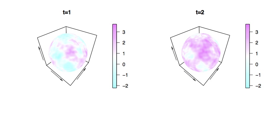
Figure 1: Simulated space-time data from the double Karhunen–Loève expansion used by Clarke et al., (2016), using 17,000 spatial sites on $\mathbb{S}^{2}$ and two temporal instants. The order of trunction is $50$ for both expansions.

Note how in each of the parametric families outlined in Table 1, the spatial margin $\psi_{\mathcal{S}}(d_{{\rm GC}})=\psi(d_{{\rm GC}},0)$ is an analytic function. In particular, we have that the spatial margin is either non differentiable or infinitely differentiable at the origin.

Spectral representations for stochastic processes over spheres, with the additional feature of axial symmetry, have been proposed in Jones, (1963), Narcowich, (1995), Hitczenko and Stein, (2012) and Castruccio and Stein, (2013). We are not aware of extensions of this representation to space-time, but the work in Jones, (1963) suggests that axial symmetry over the sphere coupled with temporal symmetry should be obtained by relaxing the assumption (3.3) for the processes $A_{k,\ell}$ in the expansion (3.2).

An alternative approach to model axially symmetric processes over spheres cross time is proposed in Castruccio and Guinness, (2017) on the basis of the stochastic representations in Jones, (1963).

Table 1: Parametric families of covariance functions on $\mathbb{S}^{2}\times\mathbb{R}$ obtained through the representation in Equation (3.4). Second column reports the analytic expression, where $g$ is any correlation function on the real line. An additional condition is required for the Sine Power family (refer to Porcu et al., 2016b, , for details). All of the members $\psi$ in the second column are rescaled so that $\psi(0,0)=1$. We use the abuse of notation $r$ for the great circle distance $d_{{\rm GC}}$.

Family	Analytic expression	Parameters range
Negative Binomial	$\psi(r,u)=\Big{(}\frac{1-\varepsilon}{1-\varepsilon g(u)\cos(r)}\Big{)}{}^{\tau}$	$\varepsilon\in(0,1)$, $\tau>0$
Multiquadric	$\psi(r,u)=\Big{(}\frac{(1-\varepsilon)^{2}}{1+\varepsilon^{2}-2\varepsilon g(u)\cos(r)}\Big{)}{}^{\tau}$	$\varepsilon\in(0,1)$, $\tau>0$
Sine Series	$\psi(r,u)=\frac{1}{2}{\rm e}^{g(u)\cos(r)-1}\big{(}1+g(u)\cos(r)\big{)}$
Sine Power	$\psi(r,u)=1-2^{-\alpha}\Big{(}1-g(u)\cos(r)\Big{)}{}^{\alpha/2}$	$\alpha\in(0,2]$
Adapted Multiquadric	$\psi(r,u)=\Big{(}\frac{(1+g^{2}(u))(1-\varepsilon)}{1+g^{2}(u)-2\varepsilon g(u)\cos(r)}\Big{)}{}^{\tau}$	$\varepsilon\in(0,1),\tau>0$
Poisson	$\psi(r,u)=\exp\big{(}\lambda(\cos(r)g(u)-1)\big{)}$	$\lambda>0$

3.2 Scale Mixture Representations

Scale mixtures provide a powerful and elegant way to build members of the class ${\cal P}(\mathbb{S}^{2},\mathbb{R})$. We sketch the general principle here and then report some examples. Let $F$ be a positive measure on the positive real line. Let $\psi_{\mathcal{S}}(d_{{\rm GC}};\xi)$ be a geodesically isotropic spatial covariance for any $\xi\in\mathbb{R}_{+}$. Also, let $C_{{\cal T}}(u;\xi)$ be a covariance for any $\xi$. Then, arguments in Porcu and Zastavnyi, (2011) and Gneiting et al., (2007) show that the function

$$\psi(d_{{\rm GC}},u)=\int_{\mathbb{R}_{+}}\psi_{\mathcal{S}}(d_{{\rm GC}};\xi)C_{{\cal T}}(u;\xi)F({\rm d}\xi),\qquad(d_{{\rm GC}},u)\in[0,\pi]\times\mathbb{R},$$

is a nonseparable geodesically isotropic and temporally symmetric space-time covariance function.

The scale mixture approach offers a nice interpretation in terms of the construction of the associated process. Let $\Xi$ be a random variable with probability distribution $F$ having a finite first moment. Let $X$ and $Y$ be, respectively, a purely spatial and a purely temporal Gaussian process. Also, suppose that the random variable ${\Xi}$ and the two processes are mutually independent. Let

$$Z(\boldsymbol{s},t\mid\Xi=\xi)=X(\boldsymbol{s}\xi)Y(t\xi),\qquad(\boldsymbol{s},t)\in\mathbb{S}^{2}\times\mathbb{R},$$

where $\xi$ is a realization from ${\Xi}$ and let $Z(\boldsymbol{s},t)=\mathbb{E}Z(\boldsymbol{s},t\mid\Xi)$, with expectation $\mathbb{E}$ taken with respect to $F$. Then, the covariance of $Z$ admits a scale mixture representation.

In general, it is not possible adapt the classes of nonseparable covariance functions based on scale mixtures and defined over $\mathbb{R}^{3}\times\mathbb{R}$ to the case $\mathbb{S}^{2}\times\mathbb{R}$. For instance, Gaussian scale mixtures as proposed in Schlather, (2010) cannot be implemented on the sphere because the function $C_{\mathcal{S}}(d_{{\rm GC}};\xi)=\exp(-(d_{{\rm GC}}/\xi)^{\alpha})$ is positive definite on the sphere only when $\alpha\in(0,1]$ (see Gneiting, , 2013). Some caution needs be taken when considering the scale mixture based covariances defined on Euclidean spaces by Porcu et al., (2007); Porcu and Mateu, (2007) and Fonseca and Steel, (2011), amongst others.

To illustrate some valid examples, further notation is needed. A function $f:[0,\infty)\to(0,\infty)$ is called completely monotonic if it is infinitely differentiable on the positive real line and if its $j$th order derivatives $f^{(j)}$ satisfy $(-1)^{j}f^{(j)}(t)\geq 0$, $t>0$, $j=0,1,2,\ldots$. A scale mixture argument in Porcu et al., 2016b shows that the function

$$\psi(d_{{\rm GC}},u)=\frac{\sigma^{2}}{\gamma_{{\cal T}}(u)^{3}}f\big{(}d_{{\rm GC}}\gamma_{{\cal T}}(u)\big{)},\qquad(d_{{\rm GC}},u)\in[0,\pi]\times\mathbb{R},$$ (3.5)

is a nonseparable covariance function on $\mathbb{S}^{2}\times\mathbb{R}$ provided $f$ is completely monotonic, with $f(0)=1$, and $\gamma_{{\cal T}}$ a variogram, with $\gamma_{\cal T}(0)=1$. Here, $\sigma^{2}$ denotes the variance. We consider a special case of Equation (3.5), namely

$$\psi(d_{{\rm GC}},u)=\frac{\sigma^{2}}{\left(1+\frac{|u|}{b_{T}}\right)^{3}}\exp\left(-\frac{d_{{\rm GC}}\left(1+\frac{|u|}{b_{T}}\right)}{b_{S}}\right),$$ (3.6)

which corresponds to $f(t)=\exp(-t)$, $t\geq 0$, with $\gamma_{\cal T}(u)=(1+|u|)$, $u\in\mathbb{R}$. Here, $\sigma^{2}$, $b_{S}$ and $b_{T}$ are positive parameters associated with the variance, spatial scale and temporal scale of the field, respectively. Figure 2 shows a realization using $\sigma^{2}=1$, $b_{S}=0.3$ and $b_{T}=0.5$.

Figure 2: Simulated space-time data from the covariance (3.6), over 17,000 spatial sites on $\mathbb{S}^{2}$ and 2 temporal instants.

Another scale mixture approach allows for an adaptation of the Gneiting class (Gneiting, , 2002; Zastavnyi and Porcu, , 2011). Again, Porcu et al., 2016b show how to derive a space-time covariance of the type

$$\psi(d_{{\rm GC}},u)=\frac{\sigma^{2}}{g_{[0,\pi]}(d_{{\rm GC}})^{1/2}}f\left(\frac{u}{g_{[0,\pi]}(d_{{\rm GC}})}\right),\qquad(d_{{\rm GC}},u)\in[0,\pi]\times\mathbb{R},$$ (3.7)

where $f$ is completely monotonic, with $f(0)=1$, and $g_{[0,\pi]}$ is the restriction to the interval $[0,\pi]$ of a function, $g:[0,\infty)\to\mathbb{R}_{+}$, having a completely monotonic derivative (see Porcu and Schilling, , 2011, for a description with classes of functions having this property).

We are now going to outline a new result within the scale-mixture based approach. Specifically, we consider quasi arithmetic means, as defined in Porcu et al., (2010): these allow to obtain space-time covariances with given margins in space and time. The construction is defined as

$$\psi(d_{{\rm GC}},u)={\cal Q}_{f}\left(\psi_{\mathcal{S}}(d_{{\rm GC}}),C_{{\cal T}}(u)\right),\qquad(d_{{\rm GC}},u)\in\mathbb{S}^{2}\times\mathbb{R},$$ (3.8)

where ${\cal Q}_{f}(x,y)=f\left(1/2f^{-1}(x)+1/2f^{-1}(y)\right)$, for a function $f$ that is completely monotonic on the positive real line, and having a proper inverse, $f^{-1}$, which is always well defined because completely monotonic functions are strictly decreasing. There is a wide list of such functions available and the reader is referred to Schilling et al., (2012) and to Porcu and Schilling, (2011). Quasi arithmetic means include as special case all the other means (e.g., the geometric, harmonic, and the Gini means), and the reader is referred to Porcu et al., (2010) for a complete description of this framework.

Using similar arguments as in Porcu et al., (2010), Theorem 6.3 in Appendix C shows the conditions for which $\psi$ in Equation (3.8) is a geodesically isotropic space-time covariance function.

3.3 Space-Time Compact Supports

Let $\psi$ be a member of the class ${\cal P}(\mathbb{S}^{2},\mathbb{R})$. We say that $\psi$ is dynamically compactly supported on the sphere if there exists a function $h:\mathbb{R}\to(0,c]$, with $c\leq\pi$, such that for every fixed temporal lag $u_{0}$, the function $\psi_{\mathcal{S}}(d_{{\rm GC}};u_{0})=\psi(d_{{\rm GC}},u_{0})$ is a covariance function on $\mathbb{S}^{2}$, and is compactly supported on the interval $[0,h(u_{0}))$.
Let $(x)_{+}$ denote the positive part of a real number $x$. For $\mu>0$ and $k=0,1,2,\ldots$, we define Wendland functions $\varphi_{\mu,k}$ (Wendland, , 1995) by

$$\varphi_{\mu,k}(x)=\left(1-x\right)_{+}^{\mu+k}{\mathbb{P}}_{k}\left(x\right),\qquad x\geq 0,$$ (3.9)

where ${\mathbb{P}}_{k}$ is a polynomial of order $k$. Special cases are depicted in the second column of Table 2.

Table 2: Wendland correlation $\varphi_{\mu,k}(\cdot)$ and Matérn correlation ${\cal M}_{\nu}(\cdot)$ with increasing smoothness parameters $k$ and $\nu$. $SP(k)$ means that the sample paths of the associated Gaussian field are $k$ times differentiable.

$k$	$\varphi_{\mu,k}(r)$	$\nu$	${\cal M}_{\nu}(r)$	$SP(k)$
$0$	$(1-r)^{\mu}_{+}$	$0.5$	$e^{-r}$	0
$1$	$(1-r)^{\mu+1}_{+}(1+r(\mu+1))$	$1.5$	$e^{-r}(1+r)$	1
$2$	$(1-r)^{\mu+2}_{+}(1+r(\mu+2)+r^{2}(\mu^{2}+4\mu+3)\frac{1}{3})$	$2.5$	$e^{-r}(1+r+\frac{r^{2}}{3})$	2
$3$	$(1-r)^{\mu+3}_{+}\big{(}1+r(\mu+3)+r^{2}(2\mu^{2}+12\mu+15)\frac{1}{5}\qquad$	$3.5$	$e^{-r}(1+\frac{r}{2}+r^{2}\frac{6}{15}+\frac{r^{3}}{15})$	$3$
	$\hskip 79.6678pt+r^{3}(\mu^{3}+9\mu^{2}+23\mu+15)\frac{1}{15}\big{)}\,$

We provide new results in the remainder of this subsection. Using scale mixture arguments, we can show that

$$\psi(d_{{\rm GC}},u)=\frac{\sigma^{2}}{c^{\alpha}}h(|u|)^{\alpha}\varphi_{\mu,0}\left(\frac{d_{{\rm GC}}}{h(|u|)}\right)=\frac{\sigma^{2}}{c^{\alpha}}h(|u|)^{\alpha}\left(1-\frac{d_{{\rm GC}}}{h(|u|)}\right)_{+}^{\mu},$$ (3.10)

$(d_{{\rm GC}},u)\in[0,\pi]\times\mathbb{R}$, where, for $\alpha\geq 3$ and $\mu\geq 4$, is a covariance function on $\mathbb{S}^{2}\times\mathbb{R}$ provided $h$ is positive, decreasing and convex on the positive real line, with $h(0)=c$, $0<c\leq\pi$, and $\lim_{t\to\infty}h(t)=0$. The additional technical restriction on $\mu$ and $\alpha$ is explained in Theorem 6.4 in Appendix C, where a formal proof is given. An example can better clarifly things. A potential candidate that can be used as dynamical support in (3.10) is the function $h(t)=c(1+t)^{-1/\alpha}$, $t\geq 0$, $\alpha\geq 3$ and $0<c\leq\pi$. Then, previous construction becomes

$$\psi(d_{{\rm GC}},u)=\frac{\sigma^{2}}{(1+|u|)}\left(1-\frac{d_{{\rm GC}}}{c(1+|u|)^{-1/\alpha}}\right)_{+}^{\mu},\qquad(d_{{\rm GC}},u)\in[0,\pi]\times\mathbb{R},$$ (3.11)

which shows that the spatial margin $\psi(d_{{\rm GC}},0)$ has compact support $c$. If $c=\pi$, then $\psi(d_{{\rm GC}},0)$ becomes globally supported. Note how the compact support becomes smaller as the temporal lag increases, which is a very intuitive property.

The following result characterizes a class of dynamically supported Wendland functions on the sphere cross time, being a generalization of (3.10) to arbitrary $k\in\mathbb{N}$.

Theorem 3.1.

Let $0<c\leq\pi$. Let $h:[0,\infty)\to(0,c]$, be positive, decreasing and convex on the positive real line, with $\lim_{t\to\infty}h(t)=0$. Let $k$ be a positive integer and $\alpha\geq 2k+2$. Let $\varphi_{\mu,k}$ be the Wendland function defined in Equation (3.9). Then,

$$\psi(d_{{\rm GC}},u)=\sigma^{2}h(|u|)^{\alpha}\varphi_{\mu,k}\left(\frac{d_{{\rm GC}}}{h(|u|)}\right),\qquad(d_{{\rm GC}},u)\in[0,\pi]\times\mathbb{R},$$ (3.12)

is a covariance function on the sphere cross time, provided $\mu\geq k+4$.

A more general statement involves compactly supported space-time covariance functions on the circle, where no parametric forms are imposed on the involved functions.

Theorem 3.2.

Let $\varphi:\mathbb{R}\times\mathbb{R}\to\mathbb{R}$ be a covariance functions that is symmetric in both first and second argument, such that $\varphi(x,u)=0$ whenever $|x|\geq\pi$, for all $u\in\mathbb{R}$. Call $\psi$ the restriction of $\varphi$ to the interval $[0,\pi]$ with respect to the first argument. Then, $\psi$ is a geodesically isotropic and temporally symmetric covariance function on the circle $\mathbb{S}^{1}$ cross time $\mathbb{R}$.

The above result is unfortunately insufficient to build for building compactly supported models over spheres cross time. Theorem 3.1 offers a special case with dynamically supported Wendland functions. To obtain a general assertion on the basis of Theorem 3.2, we give some hints in the research problems at the end of the manuscript.

3.4 Covariance Models under the Lagrangian framework

Environmental, atmospheric, and geophysical processes are often influenced by prevailing winds or ocean currents (Gneiting et al., , 2007). In this type of situation, the general idea of a Lagrangian reference frame applies. Alegria and Porcu, 2016a considered a simple Lagrangian framework that allows for transport effects over spheres. Namely, they consider random orthogonal $(3\times 3)$ matrices ${\cal R}$ with determinant identically equal to one, such that ${\cal R}^{-1}={\cal R}^{\top}$, with $\top$ denoting the transpose operator. Standard theory on random orthogonal rotations shows that ${\cal R}=QDQ^{-1},$ with $Q$ denoting a matrix containing the eigenvectors of ${\cal R}$, and $D$ a diagonal matrix containing the associated eigenvalues. Also, we have that each eigenvalue $\lambda_{k}$, $k=1,2,3$, can be uniquely written as $\lambda_{k}=\exp(\imath\kappa_{k})$, with $\imath$ being the unit imaginary number and $\kappa_{k}$ real, for $k=1,2,3$. Then, following Gantmacher, (1960), one can define the $t$th real power of ${\cal R}$, as

$${\cal R}^{t}=Q\big{(}{\rm diag}\left(\exp(\imath\kappa_{k}t)\right)\big{)}Q^{-1}.$$

Let $X$ be a Gaussian process on $\mathbb{S}^{2}$ with geodesically isotropic covariance $C_{\mathcal{S}}(\boldsymbol{s}_{1},\boldsymbol{s}_{2})=\psi_{\mathcal{S}}(d_{{\rm GC}}(\boldsymbol{s}_{1},\boldsymbol{s}_{2}))$. Define

$$Z(\boldsymbol{s},t)=X\left({\cal R}^{t}\boldsymbol{s}\right),\qquad\boldsymbol{s}\in\mathbb{S}^{2},t\in\mathbb{R}.$$ (3.13)

Then, the space-time covariance function with transport effect can be expressed as

$$C(\boldsymbol{s}_{1},\boldsymbol{s}_{2},u)=\mathbb{E}\big{(}C_{\mathcal{S}}(d_{{\rm GC}}({\cal R}^{u}\boldsymbol{s}_{1},\boldsymbol{s}_{2}))\big{)},\qquad\boldsymbol{s}_{1},\boldsymbol{s}_{2}\in\mathbb{S}^{2},\quad u\in\mathbb{R},$$ (3.14)

where the expectation is taken with respect to the random rotation ${\cal R}$. The fact that the resulting covariance is still geodesically isotropic in the spatial component is nontrivial and is shown formally, for some specific choice of the random rotation ${\cal R}$, in Alegria and Porcu, 2016a , at least for the case of the sphere $\mathbb{S}^{2}$. Some comments are in order. The resulting field $Z$ in Equation (3.13) is not Gaussian (it is Gaussian conditionally on ${\cal R}$ only). Also, obtaining closed forms for the associated covariance is generally difficult. Alegria and Porcu, 2016a provide some special cases.

For the specification of the random rotation ${\cal R}$ in the Lagrangian covariance (3.14), various choices can be physically motivated and justified. The reader is referrerd to Gneiting et al., (2007) for a thorough discussion. For instance, the random rotation might represent a prevailing wind as in Gupta and Waymire, (1987). It might be a the westerly wind considered by Haslett and Raftery, (1989) or again, it might be updated dynamically according to the current state of the atmosphere. Of course, the model (3.14) represents only a first step into Lagrangian modeling over spheres. The concept of transport effect should be put into a broader context, e.g. by following the discussion at pages 319–320 of Cressie and Wikle, (2011), which shows that the Lagrangian model offered here is a very special case, obtained when the spatial field is moving at a constant velocity. Innovative approaches to space-time data under transport effects can be found in Wikle et al., (2001) and Cressie et al., (2010).

3.5 Covariance Models based on Chordal Distances

On the basis of the results in Yadrenko, (1983) and Yaglom, (1987), Jun and Stein, (2007, 2008) exploit the fact that, for any covariance function $C_{\mathcal{S}}$ on $\mathbb{R}^{3}$, the function $C_{\mathcal{S}}(d_{{\rm CH}})$ is a covariance function on $\mathbb{S}^{2}$. The Matérn function (e.g., Stein, , 1999) is defined as

$${\cal M}_{\nu}(x)=\sigma^{2}\frac{2^{1-\nu}}{\Gamma(\nu)}x^{\nu}{\cal K}_{\nu}\left(x\right),\qquad x\geq 0,$$ (3.15)

where $\nu>0$ governs the mean square differentiability of the associated process $Z$ on $\mathbb{S}^{2}$, which is $k$ times mean differentiable if and only if $\nu>k$. Here, ${\cal K}_{\nu}$ is a modified Bessel function.

The Matérn model coupled with chordal distance, that is ${\cal M}_{\nu}(d_{{\rm CH}})$, is valid on $\mathbb{S}^{2}$ for any positive $\nu$. Unfortunately, arguments in Gneiting, (2013) show that ${\cal M}_{\nu}(d_{{\rm GC}})$ is a valid model on $\mathbb{S}^{2}$ only for $0<\nu\leq 1/2$, making its use impractical. Space-time models based on geodesic distance inherit this limitation. The same argument of the Matérn covariance is used in Guinness and Fuentes, (2016) and Jeong and Jun, (2015) to assert that the chordal distance might be preferable with respect to the great circle distance. For instance, a Matérn-Gneiting (Gneiting, , 2002; Porcu and Zastavnyi, , 2011) type covariance function based on chordal distance might be easily implemented. For a positive valued temporal variogram $\gamma_{{\cal T}}$ with $\gamma_{{\cal T}}(0)=1$, the function

$$C(d_{{\rm CH}},u)=\frac{\sigma^{2}}{\gamma_{{\cal T}}(u)^{3/2}}{\cal M}_{\nu}\left(\frac{d_{{\rm CH}}}{\gamma_{{\cal T}}(u)}\right),\qquad(d_{{\rm CH}},u)\in[0,2]\times\mathbb{R}$$ (3.16)

is a covariance function on $\mathbb{S}^{2}\times\mathbb{R}$ for any positive $\nu$. The spatial margin $C(d_{{\rm CH}},0)$ is of Matérn type and keeps all the desirable features in terms of differentiability at the origin.

The use of chordal distance has been extensively criticized in the literature. For instance, because the chordal distance underestimates the true distance between the points on the sphere, Porcu et al., 2016b argue that this fact has a nonnegligible impact on the estimation of the spatial scale. Moreover, Gneiting, (2013) argues that the chordal distance is counter to spherical geometry for larger values of the great circle distance, and thus may result in physically unrealistic distortions. Further, covariance functions based on chordal distance inherit the limitations of isotropic models in Euclidean spaces in modeling covariances with negative values. For instance, a covariance based on chordal distance on $\mathbb{S}^{2}$ does not allow for values lower than $-0.21\sigma^{2}$, with $\sigma^{2}$ being the variance as before. Instead, properties of Legendre polynomials (see Szegő, , 1939) imply that correlations based on geodesic distance can attain any value between $-1$ and $+1$. Another argument in favor of the great circle distance is that the differentiability of a given covariance function depending on the great circle distance can be modeled by imposing a given rate of decay of the associated $2$-Schoenberg coefficients $\{b_{k}\}_{k=0}^{\infty}$, as shown in Møller et al., (2017) or even modeling the rate of decay of the associated $2$-Schoenberg functions in (3.1), as shown by Clarke et al., (2016).

A good alternative to the model in Equation (3.16) is the space-time Wendland model based on the great circle distance, as defined through Equation (3.10). Table 2 highlights a striking connection between the two approaches, showing that Wendland functions allow for a parameterization of the differentiability at the origin in the same way that Matérn does. The compact support of the Wendland functions can imply some problems in terms of loss of accuracy of kriging predictors, as shown in Stein, (1999). However, recent encouraging results (Bevilacqua et al., , 2016) show that such a loss is negligible under infill asymptotics.

3.6 Nonstationary and Anisotropic Space-Time Covariance Functions

The literature regarding the construction of nonstationary space-time covariance functions is sparse. The works of Jun and Stein, (2007, 2008) are notable exceptions. The methods proposed by the authors are based on the coupling of the chordal distance with certain classes of differential operators. Estrade et al., (2016) have generalized the Berg-Porcu (Berg and Porcu, , 2017) representation of geodesically isotropic-temporally symmetric covariance functions on $\mathbb{S}^{d}\times\mathbb{R}$. In particular, two generalizations are obtained: an extension of the Berg-Porcu class to the case of temporally nonstationary covariances and a new class that allows for local anisotropy. Anisotropy is also considered in the tour de force by Hitczenko and Stein, (2012), on the basis of chordal distances. Anisotropic components can be induced through the use of Wigner matrices, as explained in Marinucci and Peccati, (2011).
More recently, Alegria and Porcu, 2016b have considered geodesically isotropic space-time covariance functions that allow the separation of the linear from the cyclical component in the temporal lag. The authors show that such approach offers considerable gains in terms of predictive performance, in particular in the presence of temporal cyclic components or in the presence of nonstationarities that are normally removed when detrending the data. A recent discussion about nonstationary approaches can be found in Fuglstad et al., (2015) who work under the SPDE framework.

4 Practical Approaches

4.1 Dynamical Approaches

When analyzing massive data sets arising from, for instance, remotely sensed networks or satellite constellations, climate models, or reanalysis data product, a model that fully specifies the covariance function becomes impractical. Indeed, it would require a prohibitive amount of information to be stored in the covariance matrix, as well as a prohibitive number of flops and iterations for maximizing the likelihood or exploring the posterior distribution. Hence, a compromise between inferential feasibility and model flexibility must be achieved. These limitations arise independently on the space where the random field is defined. For the case of the sphere, the drawbacks are magnified by the considerably more sparse literature on the construction of valid global space-time processes, as shown in the previous section, as well as by the extremely large size of global data.

In Euclidean spaces, a very popular approach to drastically reduce the complexity is to separate the spatial and temporal components and to describe the dynamics of the process by specifying its evolution as a function of the past. Variability is then achieved by assuming a random spatial innovation. For modeling global climate fields this approach has been further simplified by modeling the temporal dynamics through covariates only (Furrer et al., , 2007; Geinitz et al., , 2015).
The dynamical approach has received strong support from reference textbooks in space-time modelling (see e.g. Cressie and Wikle, , 2011) and recent years have also seen some development of this methodology in the context of global space-time data (Castruccio and Stein, , 2013). In this regard the EM algorithm has been efficiently implemented by Fassó et al., (2016) and successfully used at continental level for multivariate spatio temporal data (Finazzi and Fassó, , 2014). Thanks to the Matérn covariance implemented on the sphere, this code works also at the global level.

Let us assume, with no loss of generality, that the process has zero mean and that it is observed at some locations $\boldsymbol{s}_{1},\ldots,\boldsymbol{s}_{N}\in\mathbb{S}^{2}$, for equally spaced time points $t$. We denote $\boldsymbol{Z}_{t}=(Z(\boldsymbol{s}_{1},t),\ldots,Z(\boldsymbol{s}_{N},t))^{\top}$ the process at time $t$, and we specify its dynamic through the following recursive equation

$$\boldsymbol{Z}_{t}=\mathcal{E}_{t}(\boldsymbol{Z}_{t-1},\boldsymbol{Z}_{t-2},\ldots,\boldsymbol{Z}_{t-p})+\boldsymbol{\varepsilon}_{t},$$ (4.1)

where $\mathcal{E}_{t}$ incorporates the evolution of past trajectory of the process up to time $t-p$, and $\boldsymbol{\varepsilon}_{t}=(\varepsilon(\boldsymbol{s}_{1},t),\ldots,\varepsilon(\boldsymbol{s}_{n},t))^{\top}\overset{\mathrm{iid}}{\sim}\mathcal{N}(\boldsymbol{0},\boldsymbol{\Sigma})$ is an innovation vector with purely spatial global covariance matrix $\boldsymbol{\Sigma}$.

The considerable benefit of such an approach is that the spatio-temporal structure of the model is specified by the dynamical evolution $\mathcal{E}$ and the spatial innovation $\boldsymbol{\varepsilon}_{t}$. Hence, the temporal and spatial part of the model are de-coupled, and this allows for a considerably more convenient inference. Recent work on satellite data has proposed to couple the dynamical approach dimension reduction techniques, and in particular Fixed Rank Kriging (see Cressie and Johannesson, , 2008; Nguyen et al., , 2014) to further reduce the parameter dimensionality, and to achieve a fit for very large data sets (Fixed Rank Filtering, see Kang et al., , 2010; Cressie et al., , 2010). While these approaches have been very effective for interpolating large data sets, they do not explicitly account for the spherical geometry, but rather project the data on the Euclidean space. Here, we consider dynamical models for space-time global data with an explicit definition of the covariance function in $\mathbb{S}^{2}$.

A particularly appealing class of models with (4.1) is the Vector AutoRegressive model VAR($p$), defined as

$$\boldsymbol{Z}_{t}=\sum_{j=1}^{p}\boldsymbol{\Phi}_{j}\boldsymbol{Z}_{t-j}+\boldsymbol{\varepsilon}_{t},$$ (4.2)

where $\boldsymbol{\Phi}_{j}$ are $N\times N$ matrices that encode the temporal dependence at lag $t-j$. This model results in a space-time precision matrix that is block banded, and hence would greatly reduce the storage burden arising from massive data sets as shown in Section 5.

4.1.1 The Innovation Structure

While models such as (4.2) allow for a substantial computational saving, in typical climate model applications the number of locations is larger than $10,000$. Thus, even the likelihood of the innovation $\boldsymbol{\varepsilon}_{t}\overset{\mathrm{iid}}{\sim}\mathcal{N}(\boldsymbol{0},\boldsymbol{\Sigma})$ is impossible to evaluate for memory issues on a laptop. Therefore, to perform feasible inference on the full data set, additional structure on the model or spatial design of the data must be leveraged on. Castruccio and Stein, (2013) consider the Fourier transform cross longitude of an axially symmetric process, that is

$$\boldsymbol{\varepsilon}_{t}(\phi,\vartheta)=\sum_{k=0}^{\infty}e^{\imath\vartheta k}\mathfrak{f}(k;\phi)\widetilde{\varepsilon}_{t}(k;\phi),$$ (4.3)

$$\mbox{corr}\big{(}\widetilde{\boldsymbol{\varepsilon}}_{t}(k;\phi),\widetilde{\boldsymbol{\varepsilon}}_{t}(k^{\prime};\phi^{\prime})\big{)}=\delta_{k=k^{\prime}}\;\rho(k;{\phi,\phi^{\prime}}),\qquad\phi,\phi^{\prime}\in[0,\pi],\vartheta\in[0,2\pi),$$

with $\widetilde{\varepsilon}_{t}(k;\phi)$ being the Fourier process for wavenumber $k$ and latitude $\phi$. Here, $\mathfrak{f}(k;\phi)$ is the spectrum at latitude $\phi$ and wavenumber $k$, and, for any pair of latitudes $(\phi,\phi^{\prime})$, the function $\rho(k;{\phi,\phi^{\prime}})$ defines a spectral correlation (it is also called coherence). Jun and Stein, (2008) showed that there is a considerable computational benefit if the data are on a $N=N_{\phi}\times N_{\vartheta}$ (latitude $\times$ longitude) regular grid over the sphere and if the process is axially symmetric. Indeed, they showed how the resulting covariance matrix is block circulant and, most importantly, block diagonal in the spectral domain, thus requiring only $O(N_{\phi}\times N_{\vartheta}^{2})$ entries to store instead of $O(N^{2}_{\phi}\times N^{2}_{\vartheta})$, and $O(N_{\phi}\times N_{\vartheta}^{3})$ flops instead of $O(N_{\phi}^{3}\times N_{\vartheta}^{3})$. Castruccio and Stein, (2013) showed that such structure can be used to perform inference to massive data sets from computer model ensembles (in the range of $10^{7}$ to $10^{9}$ data points), by first estimating the spectrum $\mathfrak{f}(k;{\phi})$ for each of the $N_{\phi}$ latitudinal bands in parallel, and then conditionally estimating the structure of the spectral correlation $\rho(k;{\phi,\phi^{\prime}})$. This approach has been extended to analyze three-dimensional temperature profiles in a regular grid for a data set larger than one billion data points, allowing for an extension of axially symmetric models in three dimensions (Castruccio and Genton, , 2016).

The spectral approach is not just a mere strategy to simplify inference, but also a key to generalize axially symmetric processes to exhibit nonstationarities, by imposing additional structure in the process transformed in the spectral domain, while still guaranteeing positive definiteness of the corresponding covariance functions. In particular, it is still possible to retain the computational convenience of the gridded geometry while assuming nonstationary models cross longitudes. Castruccio and Genton, (2014) explored this idea by assuming that $\widetilde{\boldsymbol{\varepsilon}}_{t}(k;\phi)$ in (4.3) are correlated across frequencies, with a fully nonparametric dependence structure to be estimated using time replicates, and they showed how the axially symmetric assumption is badly violated for temperature data.

In order to allow for ocean transitions, Castruccio and Guinness, (2017) impose the spectrum $\mathfrak{f}(\cdot;\phi)$ in (4.3) to depend on longitude as well, and call it evolutionary spectrum (Priestley, , 1965). Given two spectra, $\mathfrak{f}_{i}(k;\phi)$, $i=1,2$ and a mapping $b_{{\rm land}}:[0,\pi]\times[0,2\pi)\to[0,1]$, an evolutionary spectrum is attained through the convex combination

$$\mathfrak{f}(k;{\phi,\vartheta})=\mathfrak{f}_{1}(k;\phi)b_{{\rm land}}(\phi,\vartheta)+\mathfrak{f}_{2}(k;\phi)\left\{1-b_{{\rm land}}(\phi,\vartheta)\right\},$$ (4.4)

so that $b_{{\rm land}}$ plays the role of modulating the relative contribution of the land regime. Castruccio and Guinness, (2017) showed how this approach is able to capture the majority of the nonstationarity occurring over a single latitudinal band. Recently, Jeong et al., (2017) proposed an extension to this approach to incorporate mountain ranges in the evolutionary spectrum in the context of wind fields. Even if the data are not on a regular grid, Horrell and Stein, (2015) showed that it is still possible to interpolate satellite data on a gridded structure using interpolated likelihoods to leverage on spectral methods. They propose to first perform kriging on the original observations, interpolate them over a grid, and evaluate the likelihood of these pseudo-observations.

The spectral approach to global data allows to achieve a fit for data sets of remarkable size, and allows to generalize axially symmetric models to capture longitudinal nonstationarities. Such a great improvement, however, comes at the cost of a loss of interpretability of the notion of distance. Indeed, the wavenumber $k$ differs in physical length for different latitudes. Thus, interpreting the dependence structure across latitudes is problematic, especially near the poles, where the physical distance among points is very small. Additionally, a process specified with a latitudinally varying spectrum is not, in general, mean square continuous at the poles. Conditions for regularity at these two singular points have been discussed in Castruccio and Guinness, (2017).

4.1.2 The Temporal Structure

For sufficiently aggregated data, (4.2) can be further simplified by assuming $\boldsymbol{\Phi}_{j}=$diag($\phi_{ii;j}$), so that the inference can be performed in parallel for each location. Simple diagnostics have shown that this structure is adequate for data spanning from multi-decadal to monthly data, while sub-monthly data would likely require a more sophisticated neighboring-dependent structure. A key feature of some geophysical processes is their dependence along thousands of miles. These teleconnections would require a more complex structure for $\boldsymbol{\Phi}_{k}$ that would link far away locations.

4.2 The SPDE Approach

We start with a brief description of the SPDE approach as in Lindgren et al., (2011) and Bolin and Lindgren, (2011). We skip all the mathematical details and will stick to the main idea. Clearly, we shall detail our exposition by working on the sphere. The main idea in Lindgren et al., (2011) is to evade from a direct specification of the Matérn function ${\cal M}_{\nu}$ as defined in Equation (3.15) in order to be able to work on any manifold, which of course includes the sphere $\mathbb{S}^{2}$. Taking verbatim from Lindgren et al., (2011), our main objective is to construct Matérn fields on the sphere, which is important for the analysis of global spatial and spatiotemporal models. Also, the authors note that they want to avoid to use the Matérn covariance adapted with chordal distance, in order to avoid the interpretational disadvantage of using chordal distances to determine the correlation between points.

The solution is to consider the SPDE having as solution a Gaussian field with Matérn covariance function: for a merely spatial process $X$ on $\mathbb{S}^{2}$, the authors study the SPDE defined through

$$(\kappa^{2}-\Delta)^{\alpha}X(\boldsymbol{s})={\cal W}(\boldsymbol{s}),\qquad\boldsymbol{s}\in\mathbb{S}^{2},$$ (4.5)

where $\kappa>0$, $\Delta$ is the Laplace-Beltrami operator, and ${\cal W}$ is a Gaussian white noise on the sphere. Here, the positive exponent $\alpha$ depends on the parameter $\nu$ in (3.15) as well as on the dimension of the sphere.
In order to provide a computationally convenient approximation of (4.5), Lindgren et al., (2011) find a very ingenious computationally efficient Hilbert space approximation. Namely, the weak solution to (4.5) if found in some approximation space spanned by some basis functions. The computational efficiency is then attained by imposing local basis functions, that is basis functions being compactly supported. This all boils into approximating the field $X$ with a Gaussian Markov field, $\boldsymbol{x}$, with precision matrix $\boldsymbol{Q}$. This idea is then generalized in Bolin and Lindgren, (2011) through nested SPDE models.

The SPDE approach proposed in Lindgren et al., (2011) is ingeniously coupled with hierarchical models by Cameletti et al., (2012) to provide a space-time model. Our exposition is adapted to the domain $\mathbb{S}^{2}\times\mathbb{R}$. The authors propose a model of the type

$$Z(\boldsymbol{s},t) = \boldsymbol{\Upsilon}_{t}^{\top}\boldsymbol{\beta}+W_{t}(\boldsymbol{s})+\varepsilon_{t}(\boldsymbol{s}),$$

$$W_{t}(\boldsymbol{s}) = aW_{t-1}(\boldsymbol{s})+{\cal W}_{t}(\boldsymbol{s}),\qquad(\boldsymbol{s},t)\in\mathbb{S}^{2}\times\mathbb{R}.$$

Here, $\boldsymbol{\Upsilon}_{t}$ is the vector of covariates and $\boldsymbol{\beta}$ is a parameter vector. The process $\varepsilon_{t}(\boldsymbol{s})$ expresses the measurement error at time $t$ and location $\boldsymbol{s}$ on the sphere. The latent process $W_{t}(\boldsymbol{s})$ is autoregressive over time and ${\cal W}_{t}(\boldsymbol{s})$ is a purely spatial process with Matérn covariance function as in Equation (3.15). The bridge with the SPDE approach thus comes from the following assumptions: ${\cal W}$ is approximated through a Gaussian Markov structure with a given precision matrix. The same approximation, but with another precision matrix, is then assigned to the process $W_{1}(\boldsymbol{s})$. Using the dynamic approach, Cameletti et al., (2012) shows that the whole latent process $W$ has a Gaussian Markov structure with a sparse precision matrix that can be calculated explicitly. A direct space-time formulation of the SPDE approach is also suggested in Lindgren et al., (2011).

5 Data example

The 2015 El Niño Southern Oscillation (ENSO) was registered as the most intense over the last two decades (Wolter and Timlin, , 2011). In September-October 2015, strong ENSO conditions coupled with the Indian Ocean Dipole suppressed precipitation and resulted in dry highly flammable landscape in Equatorial Asia. The extent of the haze from fires in the region was the largest recorded since 1997, and the increased particulate matter concentration over the densely populated area resulted in tens of millions of people being exposed to very unhealthy to hazardous air quality (as defined by the Pollutant Standard Index National Environment Agency, , 2016) and resulting into one of the worst environmental disasters on record. The assessment of exposure and mortality from this event is critical for the implementation of future mitigation strategies, and the estimation of these numbers with the associated uncertainty has received widespread media attention (Shannon et al., , 2016) and even official of estimates from scientific studies from local governments. While it is possible to focus on regional data to provide local exposure estimates, such simulations are very hard to perform and have been attempted only by Crippa et al., (2016), while all other studies have been focused on more affordable and readily available data on a global scale.

Here, we focus on this event using the MERRA2 reanalysis (Molod et al., , 2015) data of daily (aggregated from 3-hourly) Aerosol Optical Depth (AOD), see Figure 3 and movie in the online supplement. Values around 0.01 mean clear sky conditions, 0.4 very hazy condition and around 1 extremely toxic. We have also removed the trend, where for every point the monthly mean (location-wise) has been subtracted. We use this data set to compare different statistical models fitted globally but focused in the region of interest. The practical approaches discussed in Section 4 would allow for a full estimation over the two months (for a total of more than 12 million points), but that would not be possible with second order approaches. Therefore, we limit our analysis to the first $6$ days of October. While a detailed study would require an additional comparison in terms of exposure maps from population estimates, we decided to avoid this for the sake of simplicity and brevity.

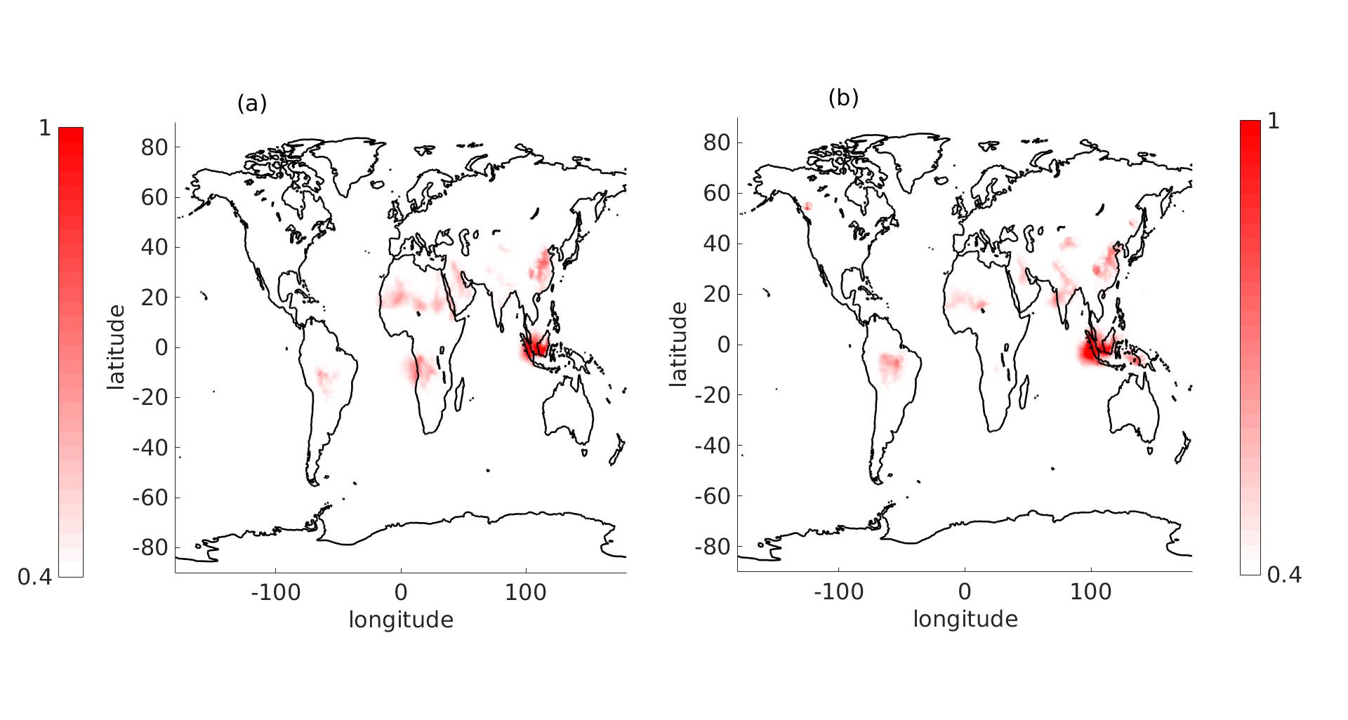
Figure 3: Averages for AOD for the months of September (a) and October (b).

5.1 The Second Order Approach

We fit the data set with a second order approach as detailed in Section 3. Despite the subsampling in time, the data set is still too large for a full analysis. Hence, a further subsampling in space a grid of 10 degrees in latitude and longitude was performed. Since several points concentred on the poles, this can produce numerical problems. We thus remove a small portion of observations, which correspond to latitudes greater than $85$ degrees and lower than $-85$ degrees.
We have considered four models:

Model 1.

A modified Gneiting covariance, as detailed by Equation (3.6).

Model 2.

A dynamically compactly supported covariance, as in Equation (3.11).

To explain the choices for Models 3 and 4, we consider the Gneiting (Gneiting, , 2002) function

$$K(r,u)=\frac{\sigma^{2}}{\left(1+\frac{r}{b_{S}}\right)^{3}}\exp\left(-\frac{|u|}{b_{T}\left(1+\frac{r}{b_{S}}\right)^{1/2}}\right).$$ (5.1)

Model 3.

A Gneiting type covariance coupled with the great circle distance, that is $\psi(d_{{\rm GC}},u)=K(d_{{\rm GC}},u))$, with $K$ as in (5.1).

Model 4.

A Gneiting type covariance $K$ as in Equation (5.1), coupled with the chordal distance, $d_{{\rm CH}}$.

The proposed models have three parameters, $(\sigma^{2},b_{S},b_{T})^{\top}$ indicating the variance, spatial and temporal range respectively. Inference was performed using a pairwise composite likelihood (CL) approach, which provides approximate but asymptotically unbiased estimates to very large data sets. We use the CL method with observations whose spatial distance is less than 6,378 kilometers (equivalent to $1$ radians on a unit sphere).

Table 3 shows CL estimates and the Log-CL value at the maximum, and both models have a similar performance in terms of CL. Figure 4 illustrates the empirical spatial (semi) variogram in terms of the great circle distance, at different temporal lags, versus the theoretical models. The models are indeed able to capture this large-scale feature of the data by fitting well the empirical variograms.

Table 3: Composite likelihood estimates, Log-CL value at the maximum and predictive scores. The units for the spatial and temporal scales are km and days, respectively.

	$\widehat{\sigma}^{2}$	$\widehat{b}_{S}$	$\widehat{b}_{T}$	Log-CL	MPSE	LSCORE	CRPS
Model 1	$8.564\times 10^{-3}$	816.38	6.320	2223640	$5.069\times 10^{-3}$	$-1.052$	$0.107$
Model 2	$8.564\times 10^{-3}$	3845.93	6.255	2223574	$5.307\times 10^{-3}$	$-0.935$	$0.106$
Model 3	$8.562\times 10^{-3}$	1651.90	2.202	2223928	$4.442\times 10^{-3}$	$-1.288$	$0.117$
Model 4	$8.563\times 10^{-3}$	765.36	5.601	2223828	$4.527\times 10^{-3}$	$-1.281$	$0.118$

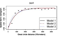
Figure 4: Empirical spatial (semi) variograms versus theoretical covariances according to Models 1, 2 and 3, at different temporal lags.

We now compare the models in terms of their predictive performance. We use the kriging predictor and a drop-one prediction strategy. We consider the following indicators: Mean Squared Prediction Error (MSPE), Log-Score (LSCORE) and Continuous Ranked Probability Score (CRPS). Table 3 contains the indicators for each model. Small values of these indicators suggest better predictions.

Models 3 and 4 produce better predictive results with respect to Models 1 and 2. In particular, Model 3 generates an approximate improvement of $2\%$ with respect to Model 4, in terms of MPSE. Model 3, based on the great circle distance, outperforms Model 4 in terms of LSCORE and CRPS.

5.2 Dynamical approach

We now fit the same data set with a dynamical model. We choose (4.2) with $p=1$, i.e., a VAR(1) process, with a diagonal autoregressive structure. Providing a location-specific temporal structure is likely to be too flexible for data subsampled for only 6 days, but further model selection approaches to reduce model complexity were deemed out of the scope of this work. Since the data are gridded, we choose a spectral model (4.3), with a latitudinally varying spectrum, and a coherence for the same wavenumber, but independence otherwise. While the model was subsampled in time for a comparison with the second-order approach, the inference was scalable and the fit of the entire data set did not require a significant additional computational time.

Even if the likelihood evaluation can sidestep the big $N$ problem by storing the results in the spectral domain via a Whittle likelihood (Whittle, , 1953), it is not possible to obtain a maximum likelihood for the entire model. Because the model’s structure, comprising of hundreds of parameters, the optimization over the entire space would be impossible. Therefore, the estimation is performed step-wise. First, the temporal dependence is estimated. Then, we estimate the longitudinal dependence, then the latitudinal dependence, and hence the parameter estimates are to be regarded as local approximations.

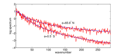
Figure 5: Fitted parametrical (blue) and non parametrical (i.e., periodogram red) log spectrum for two different latitudinal bands, one at the equator, one at high northern latitudes. The periodogram was obtained by averaging across all longitudes and times.

The spectral model allows for a different spectral shape at different latitudes, and it is flexible enough to capture very different behaviours, as illustrated in Figure 5. Indeed, AOD residuals near the equator display a much smoother behaviour than at high latitudes, where the spectrum is more flat, but the model is able to fit both behaviours naturally.

5.3 Comparison for Equatorial Asia

While both models are fitted globally, the interest lies in their relative performance in the area of interest, i.e., in Equatorial Asia. Table 4 shows a comparison of the aforementioned models in terms of the marginal likelihood in this area, defined as all points whose latitudes is between $-11.3$ and $15.3$ degrees ($N_{\phi}=53$) and whose longitude is between $93$ to $137$ degrees ($N_{\vartheta}=71$). The dynamically specified model outperforms almost uniformly Models 1 and 2 in the second order approach: it is faster, richer in complexity yet achieving a overwhelmingly better fit, so it is clearly more suitable for a more detailed analysis in the area.

While these results are strongly in favor of the dynamically approach, it must be pointed out that the particular setting of the global space-time data analyzed, i.e., a regular grid in space and equal observations in time, is such that a spectral model is clearly the best choice. An application with more complicated geometries such as with satellite data, would have required an adaptation of spectral methods along the lines of Horrell and Stein, (2015) and, likely, a worse fit. While such a comparison with an irregular design would have been added to the discussion, we decided to avoid it for the sake of brevity.

Table 4: Comparison between different models in terms of number of parameters (excluding the temporal ones), computational time (minutes), normalized loglikelihood, and Bayesian Information Criterion for $K=6$ days from October 1st to October 6th 2015.

	$\#$ param	Time (minutes)	$\Delta$-loglik$/(N_{\phi}N_{\vartheta}K)$	BIC$\times 10^{4}$
Model 1	$3$	$238$	$-3.24$	$-4.50$
Model 2	$3$	$236$	$-3.24$	$-4.55$
Model (4.3)	$161$	$4.2$	$0$	$-19.0$

6 Research Problems

This section is devoted to a list of research problems that we consider relevant for future researches.

1. Nonstationary Space-Time Covariances.

The models proposed in Section 3 are geodesically isotropic and temporally symmetric. Since real phenomena on the globe are notably nonstationary, it is necessary to use those models as building blocks for more sophisticated constructions. In particular, the development of nonstationary models is necessary and a promising direction of research is to extend the work of Guella et al., (2017); Guella et al., 2016b ; Guella et al., 2016a who define kernels over products of $n$-dimensional spheres. Another direction of research might be to take into account differences in local geometry of the sphere representing planet Earth. Thus, the natural solution is to work on processes evolving temporally over Riemannian manifolds. In this direction, the works of Menegatto et al., (2006) and the recent work by Barbosa and Menegatto, (2017) might be very useful.

2. Models based on Convolutions.

Convolution arguments have been used for Gaussian processes defined over spheres (no time) in order to index the associated fractal dimension. Hansen et al., (2015) show that Gaussian particles provide a flexible framework for modelling and simulating three-dimensional star-shaped random sets. The authors show that, if the kernel is a von Mises-Fisher density, or uniform on a spherical cap, the correlation function of the associated random field admits a closed form expression. We are not aware of any convolution argument for space-time covariance functions. The work of Ziegel, (2014) might be very useful in this direction.

3. Physical-based Constructions.

Constructions based on dynamical models or moving averages have been proposed by Ailliot et al., (2011) and Schlather, (2010). We are not aware of such extensions to the case $\mathbb{S}^{2}\times\mathbb{R}$, but certainly it would be worth being studied. Some other constructions based on physical characteristic of the space-time process might be appealing for modeling several real processes. In this direction, it would be desirable to study the approaches proposed in Christakos, (2000) as well as Kolovos et al., (2004); Christakos, (1991); Christopoulos and Tsantili, (2016) and Christakos et al., 2000a .

4. Multivariate Space-Time Models.

Often, several variables are observed over the same spatial location and same temporal resolution. Thus, there is substantial need of space-time multivariate covariance models being geodesically isotropic or axially symmetric in the spatial component. The literature in this subject is very sparse, with the notable exceptions of Jun and Stein, (2008) and Alegria et al., (2017).

5. Matérn Analogues over Spheres.

Find the counterpart of the Matérn covariance function on the sphere. This would allow to have a covariance function that indexes the differentiability at the origin of the associated Gaussian field. Notable attempts have been made by Guinness and Fuentes, (2016), with partial success. Møller et al., (2017) suggest to model the $n$-Schoenberg coefficients (see Appendix A for details) imposing a given rate of decay, but this does not allow for explicit closed forms.

5. Compact Supports with Differentiable Temporal Margins.

A potential drawback of the space-time construction as in Theorem 3.1 is that it only allows for temporal margins being non differentiable at the origin. An important step ahead would be to improve such a limitation. Following the arguments in the proof of Theorem 3.1, the crux would be in proving that, for some mapping $h:[0,\infty)\to\mathbb{R}$, the function

$$h(u^{2})^{\alpha+d}\mathstrut_{1}F_{2}\bigg{\{}1+k;\frac{\mu+2}{2}+k,\frac{\nu+3}{2}+k;-n^{2}h(u^{2})^{2}/4\bigg{\}},\qquad u\in\mathbb{R},\quad n\in\mathbb{N},$$

is positive definite for all $n\in\mathbb{N}$.

6. Spectral Constructions à la Stein.

Stein, 2005a proposes a class of spectral densities in $\mathbb{R}^{d}\times\mathbb{R}$ of the type

$$\mathfrak{f}(\boldsymbol{\omega},\tau)=\left((1+\|\boldsymbol{\omega}\|)^{\alpha_{1}}+(1+|\tau|)^{\alpha_{2}}\right)^{-\alpha_{3}},\qquad(\boldsymbol{\omega},\tau)\in\mathbb{R}^{d}\times\mathbb{R},\quad\alpha_{i}>0,$$

for $i=1,2,3$. Under the condition $\alpha_{3}<\alpha_{1}/d+\alpha_{2}$, $\mathfrak{f}$ is in $L_{1}(\mathbb{R}^{d}\times\mathbb{R})$. The partial Fourier transforms allow for indexing the differentiability at the origin in a similar way as the Matérn covariance function. Further, the resulting covariance is smoother away from the origing than at the origin, which is important as reported in Theorem 1 in Stein, 2005a . There is no analogue of $\mathfrak{f}$-based constructions for the class ${\cal P}(\mathbb{S}^{2},\mathbb{R})$. One should necessarily start from Berg-Porcu (Berg and Porcu, , 2017) characterization and try to find a related approach that allows to obtain such a construction on spheres cross time.

7. Local Anisotropies and Transport Effects.

The geodesically isotropic models should be extended to allow for local anisotropies as in Paciorek and Schervish, (2006). In this direction, a major step should be made in order to generalize the Lagrangian model in Equation (3.14) to the nonstationary case.

8. Strictly Positive Definite Functions.

A function $C:(\mathbb{S}^{2}\times\mathbb{R})^{2}\to\mathbb{R}$ is called strictly positive definite when inequality

$$\sum_{i,j}^{N}c_{i}C\big{(}(\boldsymbol{s}_{i},t_{i}),(\boldsymbol{s}_{j},t_{j})\big{)}c_{j}>0,$$

holds for any $\{c_{k}\}_{k=1}^{N}\subset\mathbb{R}$, unless $c_{1}=\dots=c_{N}=0$, and $\{\boldsymbol{s}_{k},t_{k}\}_{k=1}^{N}\subset\mathbb{S}^{d}\times\mathbb{R}$. There is substantial work on strict positive definiteness and the reader is referred to Chen et al., (2003); Menegatto, (1994, 1995) and Menegatto et al., (2006). A characterization of the subclass of ${\cal P}(\mathbb{S}^{n},\mathbb{R})$ (see Appendix A) with members $\psi$ such that the corresponding covariances $C$ are strictly positive definite is still elusive.

9. Walks through Dimensions.

The literature on walks through dimensions is related to operators that allow, for a given positive definite function on the $n$-dimensional sphere, to obtain new classes of positive definite functions on $n^{\prime}$-dimensional spheres, with $n\neq n^{\prime}$. The application of such operators has consequences on the differentiability at the origin of the involved functions. Walks on spheres have been proposed by Beatson et al., (2014), Ziegel, (2014) and by Massa et al., (2017), this last extending previous work to the case of complex spheres. It would be timely to obtain walks through dimensions for the members of the classes ${\cal P}(\mathbb{S}^{n},\mathbb{R})$, for $n$ a positive integer.

10. Optimal Prediction on Spheres cross Time.

Much work needs to be done in order to assess asymptotic optimal kriging prediction over spheres cross time when the covariance is missspecified. The work of Arafat et al., (2016) opens a bridge between equivalence of Gaussian measures and asymptotic optimal prediction over spheres. A relevant direction of research would be to evaluate the screening effect on spheres cross time. After the works of Stein, (1999), there is nothing related to spectral behaviours over spheres that allow for evaluating the corresponding screening effect.

11. Fast Simulations on Spheres.

Lang and Schwab, (2013) and Clarke et al., (2016) propose fast simulations through truncation of Karhunen-Loève expansions. It would be very interesting to propose analogues of circulant embedding methods, where the difficulty is mainly due to the fact that it is not possible to set a regular grid on the sphere.

12. Chordal vs Great Circle Again.

Moreno Bevilacqua (personal communication) points out that he has tried the following experiment. Simulate any set of points on the sphere cross time. Take any element $\psi$ from the class ${\cal P}(\mathbb{S}^{2},\mathbb{R})$. Replace the great circle distance with the chordal distance and calculate the corresponding matrix realizations. With all the experiments, he always found strictly positive eigenvalues. Thus, the question is: suppose that $\psi\in{\cal P}(\mathbb{S}^{2},\mathbb{R})$. Then, is it true that $\psi(d_{{\rm CH}})$ is positive definite on $\mathbb{S}^{2}\times\mathbb{S}^{2}\times\mathbb{R}$?

Appendix

Appendix A: Mathematical Background

We need some notation in order to illustrate the following sections. This material follows largely the exposition in Berg and Porcu, (2017).

Let $n$ be a positive integer. We denote $\mathbb{S}^{n}$ the $n$-dimensional unit sphere of $\mathbb{R}^{n+1}$, given as

$$\mathbb{S}^{n}=\{\boldsymbol{s}\in\mathbb{R}^{n+1}\mid\|\boldsymbol{s}\|=1\},\;n\geq 1.$$ (6.1)

We also consider

$$\mathbb{S}^{\infty}=\{(s_{k})_{k\in\mathbb{N}}\in\mathbb{R}^{\mathbb{N}}|\sum_{k=1}^{\infty}s_{k}^{2}=1\},$$

which is the unit sphere in the Hilbert sequence space $\ell_{2}$ of square summable real sequences. Following Berg and Porcu, (2017), we thus define the class ${\cal P}(\mathbb{S}^{n},\mathbb{R})$ as the class of continuous functions $\psi:[0,\pi]\times\mathbb{R}\to\mathbb{R}$ such that

$$C\big{(}(\boldsymbol{s}_{1},t_{1}),(\boldsymbol{s}_{2},t_{2})\big{)}=\psi(d_{{\rm GC}}(\boldsymbol{s}_{1},\boldsymbol{s}_{2}),t_{1}-t_{2}),\qquad(\boldsymbol{s}_{i},t_{i})\in\mathbb{S}^{n}\times\mathbb{R},\quad i=1,2,$$

where $d_{{\rm GC}}$ as already been defined as the great circle distance. Berg and Porcu, (2017) define ${\cal P}(\mathbb{S}^{\infty},\mathbb{R})$ as $\bigcap_{n\geq 1}{\cal P}(\mathbb{S}^{n},\mathbb{R})$. The inclusion relation

$${\cal P}(\mathbb{S}^{1},\mathbb{R})\supset{\cal P}(\mathbb{S}^{2},\mathbb{R})\supset\cdots\supset{\cal P}(\mathbb{S}^{\infty},\mathbb{R})$$

is strict and the reader is referred to Berg and Porcu, (2017) for details.

We recall the definition of Gegenbauer polynomials $C_{k}^{(\lambda)}$, given by the generating function (see Dai and Xu, , 2013)

$$(1-2xz+r^{2})^{-\lambda}=\sum_{k=0}^{\infty}C_{k}^{(\lambda)}(z)r^{k},\quad|r|<1,z\in\mathbb{C}.$$ (6.2)

Here, $\lambda>0$. We have the classical orthogonality relation:

$$\int_{-1}^{1}(1-x^{2})^{\lambda-1/2}C_{k}^{(\lambda)}(x)C_{h}^{(\lambda)}(x)\,{\rm d}x=\frac{\pi\Gamma(k+2\lambda)2^{1-2\lambda}}{\Gamma^{2}(\lambda)(k+\lambda)k!}\delta_{h=k},$$ (6.3)

with $\Gamma$ denoting the Gamma function.
It is of fundamental importance that $|C_{k}^{(\lambda)}(x)|\leq C_{k}^{(\lambda)}(1)$, $x\in[-1,1]$. The special value $\lambda=(n-1)/2$ is relevant for the sphere $\mathbb{S}^{n}$ because of the relation to spherical harmonics, which is illustrated in Berg and Porcu, (2017) as follows. A spherical harmonic of degree $k$ for $\mathbb{S}^{n}$ is the restriction to $\mathbb{S}^{n}$ of a real-valued harmonic homogeneous polynomial in $\mathbb{R}^{n+1}$ of degree $k$. Together with the zero function, the spherical harmonics of degree $k$ form a finite dimensional vector space denoted $\mathcal{H}_{k}(n)$. It is a subspace of the space ${\mathcal{C}}(\mathbb{S}^{n})$ of continuous functions on $\mathbb{S}^{n}$. We have

$$N_{k}(n):=\dim\mathcal{H}_{k}(n)=\frac{(n)_{k-1}}{k!}(2n+n-1),\;k\geq 1,\quad N_{0}(n)=1,$$ (6.4)

(see Dai and Xu, , 2013, p.3). Here, $(n)_{k-1}$ denotes the Pochammer symbol.
The surface measure of the sphere is denoted $\omega_{n}$, and it has total mass

$$||\omega_{n}||=\frac{2\pi^{(n+1)/2}}{\Gamma((n+1)/2)}.$$ (6.5)

The spaces $\mathcal{H}_{k}(n)$ are mutual orthogonal subspaces of the Hilbert space $L^{2}(\mathbb{S}^{n},\omega_{n})$, which they generate. This means that any $F\in L^{2}(\mathbb{S}^{n},\omega_{n})$ has an orthogonal expansion

$$F=\sum_{k=0}^{\infty}S_{k},\,S_{k}\in\mathcal{H}_{k}(n),\quad||F||_{2}^{2}=\sum_{k=0}^{\infty}||S_{k}||_{2}^{2},$$ (6.6)

where the first series converges in $L^{2}(\mathbb{S}^{n},\omega_{n})$, and the second series is Parseval’s equation (Berg and Porcu, , 2017). Here $S_{k}$ is the orthogonal projection of $F$ onto $\mathcal{H}_{k}(n)$ given as

$$S_{k}(\xi)=\frac{N_{k}(n)}{||\omega_{n}||}\int_{\mathbb{S}^{n}}c_{k}(n,\langle\boldsymbol{s},\eta\rangle)F(\eta)\,{\rm d}\omega_{n}(\eta).$$ (6.7)

See the addition theorem for spherical harmonics, (Schoenberg, , 1942). For $\lambda=(n-1)/2$, $c_{k}(n,x)$ is defined as the normalized Gegenbauer polynomial

$$c_{k}(n,x)=C_{k}^{((n-1)/2)}(x)/C_{k}^{((n-1)/2)}(1)=\frac{k!}{(n-1)_{k}}C_{k}^{((n-1)/2)}(x),$$ (6.8)

being 1 for $x=1$.
Specializing the orthogonality relation (6.3) to $\lambda=(n-1)/2$ and using Equations (6.4), (6.5), Berg and Porcu, (2017) get for $n\in\mathbb{N}$

$$\int_{-1}^{1}(1-x^{2})^{n/2-1}c_{k}(n,x)c_{h}(n,x)\,{\rm d}x=\frac{||\omega_{n}||}{||\omega_{n-1}||N_{k}(n)}\delta_{h=k}.$$ (6.9)

The following result characterizes completely the class ${\cal P}(\mathbb{S}^{n},\mathbb{R})$.

Theorem 6.1.

(Berg and Porcu, , 2017). Let $n\in\mathbb{N}$ and let $\psi:[0,\pi]\times\mathbb{R}\to\mathbb{C}$ be a continuous function. Then $\psi$ belongs to the class ${\cal P}(\mathbb{S}^{n},\mathbb{R})$ if and only if there exists a sequence $\{\varphi_{k,n}\}_{k=0}^{\infty}$ of positive definite functions on $\mathbb{R}$, with $\sum\varphi_{k,n}(0)<\infty$, such that such that

$$\psi(d_{{\rm GC}},u)=\sum_{k=0}^{\infty}\varphi_{k,n}(u)c_{k}(n,\cos d_{{\rm GC}}),$$ (6.10)

and the above expansion is uniformly convergent for $(d_{{\rm GC}},u)\in[0,\pi]\times\mathbb{R}$. We have

$$\varphi_{k,n}(u)=\frac{N_{k}(n)||\omega_{n-1}||}{||\omega_{n}||}\int_{0}^{\pi}\psi(x,u)c_{k}(n,x)\sin x^{n-1}\,{\rm d}x.$$ (6.11)

We also report the characterization of the class ${\cal P}(\mathbb{S}^{\infty},\mathbb{R})$ obtained by the same authors.

Theorem 6.2.

(Berg and Porcu, , 2017) Let $\psi:[0,\pi]\times\mathbb{R}\to\mathbb{R}$ be a continuous function. Then $\psi$ belongs to ${\cal P}(\mathbb{S}^{\infty},\mathbb{R})$ if and only if there exists a sequence $\{\varphi_{k}\}_{k=0}^{\infty}$ of positive definite functions on $\mathbb{R}$, with $\sum_{k}\varphi_{k}(0)<\infty$ such that

$$\psi(d_{{\rm GC}},u)=\sum_{k=0}^{\infty}\varphi_{k}(u)\cos^{k}d_{{\rm GC}},$$ (6.12)

and the above expansion is uniformly convergent for $(d_{{\rm GC}},u)\in[0,\pi]\times G$.

Some comments are in order. Theorems 6.1 and 6.2 are fundamental to create the examples illustrated in Table 1. Also, they are crucial to solve some of the open problems that we reported in Section 6. Table 5 lists some permissible models on $\mathbb{S}^{2}\times\mathbb{R}$.

Table 5: Parametric families of geodesically isotropic space-time covariance functions. PMC is the acronym for Porcu-Mateu-Christakos Porcu et al., (2010). PBG is the acronym for Porcu-Bevilacqua-Genton Porcu et al., 2016b . We use the abuse of notation $r$ for the great circle distance $d_{{\rm GC}}$.

Family	Expression for $\psi(r,u)$	Parameter Restrictions
Fonseca-Steel	$\displaystyle\frac{1+(\gamma_{\mathcal{S}}(r)+\gamma_{{\cal T}}(u))}{(1+\gamma_{\mathcal{S}}(r)\big{)}^{\lambda_{1}}}\frac{{\cal K}_{\lambda_{1}}\left(2\sqrt{(a+\gamma_{\mathcal{S}}(r))^{\delta}}\right)}{{\cal K}_{\lambda_{1}}(2\sqrt{a\delta})}$	$a_{1},\delta,\lambda_{i}>0$, $i=0,1$.
Clayton PMC	$\bigg{(}(1+r^{\alpha})^{\rho_{1}}+(1+|u|^{\beta})^{\rho_{2}}-1\bigg{)}^{-\rho_{3}}$	$\alpha,\beta,\rho_{1},\rho_{2}\in(0,1]$; $\rho_{3}>0$.
Gumbel PMC	$\exp\bigg{(}-\left(r^{\alpha_{1}}+u^{\alpha_{2}}\right)^{\alpha_{3}}\bigg{)}$	$\alpha_{i}\in(0,1]$, $i=1,2,3$.
PBG	Equation (3.5)
Families for $f$ Expression Parameters Dagum $f(r)=1-\left(\frac{r^{\beta}}{1+r^{\beta}}\right)^{\tau}$ $\beta,\tau\in(0,1]$ Matérn Equation (3.15) $0<\nu\leq 1/2$ Gen. Cauchy $f(r)=(1+r^{\alpha})^{-\beta/\alpha}$ $\alpha\in(0,1]$, $\beta>0$ Pow. Exponential $f(r)=\exp(-r^{\alpha})$ $\alpha\in(0,1]$
Adaptive Gneiting	Equation (3.7)	$f$ as in PBG family
Families for $g_{[0,\pi]}$ Expression Parameters Dagum $g_{[0,\pi]}(r)=1+\left(\frac{r^{\beta}}{1+r^{\beta}}\right)^{\tau}$ $\beta,\tau\in(0,1]$ Gen. Cauchy $g_{[0,\pi]}(r)=(1+r^{\alpha})^{\beta/\alpha}$ $\alpha\in(0,1]$, $\beta\leq\alpha$ Power $g_{[0,\pi]}(r)=c+r^{\alpha}$ $\alpha\in(0,1]$, $c>0$
PBG2	Equation (3.10)	$h$ positive, decreasing and
		convex with $\lim_{t\to\infty}h(t)=0$.
Dynamical Wendland	Equation (3.12)	$h$ positive, decreasing and
		convex with $\lim_{t\to\infty}h(t)=0$.
Families for $\varphi_{\mu,k}$ Expression Parameters Dynamical Wendland 2 $h(|u|)^{\alpha}\left(1-\frac{r}{h(|u|)}\right)_{+}^{6}\left(1+6\frac{r}{h(|u|)}\right)$ $\alpha\geq 4$ Dynamical Wendland 4 $h(|u|)^{\alpha}\left(1-\frac{r}{h(|u|)}\right)_{+}^{8}\left(1+8\frac{r}{h(|u|)}+\frac{63}{3}\left(\frac{r}{h(|u|)}\right)^{2}\right)$ $\alpha\geq 4$

Appendix C. Mathematical Proofs

C1. The Quasi Arithmetic Class on Spheres

For ease of exposition, we slightly deviate from the notation of the paper and denote $f\circ g$ the composition of $f$ to $g$. Let us recall the expression of quasi arithmetic covariances as in Equation (3.8):

$$\psi(d_{{\rm GC}},u)=f\left(\frac{1}{2}f^{-1}\circ\psi_{\mathcal{S}}(d_{{\rm GC}})+\frac{1}{2}f^{-1}\circ C_{{\cal T}}(u)\right),\qquad(d_{{\rm GC}},u)\in[0,\pi]\times\mathbb{R}.$$

By Bernstein’s theorem (Feller, , 1966, p. 439), a function $f:[0,\infty)\to\mathbb{R}$ is completely monotonic if and only if

$$f(t)=\int_{[0,\infty)}{\rm e}^{-\xi t}H({\rm d}\xi),\qquad t\geq 0,$$ (6.13)

where $H$ is a positive and bounded measure. A Bernstein function is a continuous mapping on the positive real line, having a first derivative being completely monotonic. We are now able to give a formal assertion for the validity of the quasi arithmetic construction.

Theorem 6.3.

Let $f:[0,\infty)\to\mathbb{R}_{+}$ be a completely monotonic function. Let $f_{1}:[0,\infty)\to\mathbb{R}$ be a continuous functions such that $f^{-1}\circ f_{1}$ is a Bernstein function. Let $C_{{\cal T}}:\mathbb{R}\to\mathbb{R}$ be a continuous, symmetric covariance function such $f^{-1}\circ C_{{\cal T}}$ is a temporal variogram. Call $\psi_{\mathcal{S}}=f_{1,[0,\pi]}$ the restriction of $f_{1}$ to the interval $[0,\pi]$. Then,

$$\psi(d_{{\rm GC}},u)={\cal Q}_{f}\left(\psi_{\mathcal{S}}(d_{{\rm GC}}),C_{{\cal T}}(u)\right),\qquad(d_{{\rm GC}},u)\in[0,\pi]\times\mathbb{R},$$ (6.14)

is a geodesically isotropic space-time covariance function on $\mathbb{S}^{n}\times\mathbb{R}$, for all $n=1,2,3,\ldots$.

Proof.

Denote $g$ the composition $f^{-1}\circ f_{1}$ and call $g_{[0,\pi]}$ the restriction of $g$ to $[0,\pi]$, obtained through $g_{[0,\pi]}=f^{-1}\circ f_{1,[0,\pi]}$. By assumption, $g$ is a Bernstein function. Thus, arguments in Porcu and Schilling, (2011), with the references therein, show that the function $h$, defined through

$$h(t;\xi)=\exp(-\xi g(t)),\qquad t,\xi\geq 0,$$

is a completely monotonic fuction for any positive $\xi$. Thus,

$$h_{[0,\pi]}(d_{{\rm GC}};\xi)=\exp\left(-\xi f^{-1}\circ f_{1,[0,\pi]}(d_{{\rm GC}})\right),\qquad d_{{\rm GC}}\in[0,\pi],$$

is the restriction of a completely monotonic function to the interval $[0,\pi]$. Invoking Theorem 7 in Gneiting, (2013), we obtain that $h_{[0,\pi]}$ is a geodesically isotropic covariance function on any $n$-dimensional sphere. Additionally, since $f^{-1}\circ C_{{\cal T}}$ is a temporal variogram, by Schoenberg’s theorem (Schoenberg, , 1938) we deduce that $k(u;\xi)=\exp(-\xi f^{-1}\circ C_{{\cal T}}(u))$, $u\in\mathbb{R}$, is a covariance function on the real line for every positive $\xi$. Thus, the scale mixture covariance

$$\psi(d_{{\rm GC}},u) = \int_{[0,\infty)}h_{[0,\pi]}(d_{{\rm GC}};\xi)k(u;\xi)H({\rm d}\xi)$$

$$= \int_{[0,\infty)}\exp\left(-\xi g_{[0,\pi]}(d_{{\rm GC}})-\xi f^{-1}\circ C_{{\cal T}}(u)\right)H({\rm d}\xi)$$

$$= {\cal Q}_{f}(\psi_{\mathcal{S}}(d_{{\rm GC}}),C_{{\cal T}}(u)),\qquad(d_{{\rm GC}},u)\in[0,\pi]\times\mathbb{R},$$

is a covariance function on $\mathbb{S}^{n}\times\mathbb{R}$ for all $n\in\mathbb{N}$. ∎

C2. Proofs for Section 3.3

Theorem 6.4.

Let $h$ be a positive, decreasing and convex function on the positive real line, with $h(0)=c$, $0<c\leq\pi$, and $\lim_{t\to\infty}h(t)=0$. Let $\alpha\geq 3$ and $\mu\geq 4$. Then, Equation (3.10) defines a geodesically isotropic and temporally symmetric covariance function on $\mathbb{S}^{3}\times\mathbb{R}$.

Proof.

The proof is based on scale mixture arguments in concert with the calculations in Porcu et al., 2016a . In particular, we have that the function in Equation (3.10) is the result of the scale mixture of the function $\psi_{\mathcal{S}}(d_{{\rm GC}};\xi)=(1-d_{{\rm GC}}/\xi)_{+}^{n}$ with the function $C_{{\cal T}}(u;\xi)=\xi^{n}\left(1-\frac{\xi}{h(|u|)}\right)_{+}^{\gamma}$, $\xi>0,t\geq 0$, $\gamma\geq 1,n\geq 2$. In particular, arguments in Lemmas 3 and 4 in Gneiting, (2013) show that $\psi_{\mathcal{S}}$ is a covariance function on $\mathbb{S}^{3}$ for every positive $\xi$. Under the required conditions on the function $h$, we have that $C_{{\cal T}}$ is a covariance function on $\mathbb{R}$ for every positive $\xi$. Thus, the scale mixture arguments in Porcu et al., 2016a , with $\mu=n+\gamma+1$ and $\alpha=n+1$ can now be applied, obtaining the result. ∎

A more sophisticated argument is required to show that the structure in Equation (3.12) is positive definite on the circle cross time. We start with the proof of Theorem 3.2 because its arguments will be partially used to prove Theorem 3.1.

Proof of Theorem 3.2.

Denote $\varphi_{[0,\pi]}$ the restriction of $\varphi$ to the interval $[0,\pi]$ with respect to the first argument. Let $n\in\mathbb{N}$. Consider the sequence of functions $b_{n}(\cdot)$, defined through

$$b_{n}(u) = \frac{2}{\pi}\int_{0}^{\pi}\cos(nz)\psi(z,u){\rm d}z=\frac{2}{\pi}\int_{0}^{\pi}\cos(nz)\varphi_{{[0,\pi]}}(z,u){\rm d}z$$ (6.15)

$$= \frac{1}{\pi}\int_{-\infty}^{\infty}\cos(nx)\varphi(x,u){\rm d}x.$$

Since $\varphi$ is positive definite on $\mathbb{R}\times\mathbb{R}$, arguments in Lemma 1 in Gneiting, (2002) show that $b_{n}(u)$ is a covariance function on $\mathbb{R}$ for all $n\in\mathbb{N}$. Additionally, we have

$$\sum_{n=0}^{\infty}b_{n}(0)=\sum_{n=0}^{\infty}\frac{1}{\pi}\int_{-\infty}^{\infty}\cos(nx)\varphi(x,0){\rm d}x=\sum_{n=0}^{\infty}\widehat{\varphi}_{\mathbb{N}}(n)<\infty,$$

where $\widehat{\varphi}_{\mathbb{N}}$ denotes the Fourier transform of $\varphi(x,0)$ restricted to natural numbers. Thus, we get that $\sum_{n}b_{n}(0)<\infty$ because the Fourier transform of a positive definite function is nonnegative and integrable. We can thus invoke Theorem 3.3 in Berg and Porcu, (2017) to obtain that $\psi(d_{{\rm GC}},u)=\varphi_{[0,\pi]}(d_{{\rm GC}},u)$ is a covariance function on the circle $\mathbb{S}^{1}$ cross time. ∎

Proof of Theorem 3.1.

We give a proof of the constructive type. Let $k\in\mathbb{N}$. Arguments in Theorem 1 of Porcu et al., 2016a show that the function

$$C(x,u)=\sigma^{2}h(|u|)^{\alpha}\varphi_{\mu,k}\left(\frac{|x|}{h(|u|)}\right),\qquad(x,u)\in\mathbb{R}\times\mathbb{R},$$ (6.16)

is positive definite on $\mathbb{R}\times\mathbb{R}$ provided $\alpha\geq 2k+3$ and $\mu\geq k+4$. Arguments in Porcu et al., 2016c show that

$$b_{n}(u) = \int_{{}_{\infty}}^{-\infty}\cos(nx)C(x,u){\rm d}x$$

$$\propto \sigma^{2}h(|u|)^{\alpha+d}\mathstrut_{1}F_{2}\bigg{(}1+k;\frac{\mu+2}{2}+k,\frac{\nu+3}{2}+k;-n^{2}h(|u|)^{2}/4\bigg{)},\qquad u\in\mathbb{R},\quad n\in\mathbb{N}.$$

From the argument in (6.15) in concert with Lemma 1 in Gneiting, (2002), we have that $b_{n}(u)$ is positive definite on the positive real line for each $n$. Additionally, arguments in Porcu et al., 2016c show that, for $\mu\geq k+4$, $b_{n}(u)$ is strictly decreasing in $n$. Application of Proposition 3.6 of Berg and Porcu, (2017) shows that (3.12) is positive definite on $\mathbb{S}^{3}\times\mathbb{R}$. ∎

References

- Ailliot et al., (2011) Ailliot, P., Baxevani, A., Cuzol, A., Monbet, V., and Raillard, N. (2011). Space-Time Models for Moving Fields with an Application to Significant Wave Height Fields. Environmetrics, 22(3):354–369.
- (2) Alegria, A. and Porcu, E. (2016a). The Dimple Problem related to Space-Time Modeling under the Lagrangian Framework. Technical Report, University Federico Santa Maria.
- (3) Alegria, A. and Porcu, E. (2016b). Space-Time Geostatistical Models with both Linear and Seasonal Structures in the Temporal Components. Technical Report, University Federico Santa Maria.
- Alegria et al., (2017) Alegria, A., Porcu, E., Furrer, R., and Mateu, J. (2017). Covariance Functions for Multivariate Gaussian Fields Evolving Temporally over Planet Earth. Technical Report, University Federico Santa Maria.
- Arafat et al., (2016) Arafat, A., Porcu, E., Bevilacqua, M., and Mateu, J. (2016). Equivalence and Orthogonality of Gaussian Measures on Spheres. Technical Report, University Federico Santa Maria.
- Baldi and Marinucci, (2006) Baldi, P. and Marinucci, D. (2006). Some Characterizations of the Spherical Harmonics Coefficients for Isotropic Random Fields. Statistics and Probability Letters, 77:490–496.
- Banerjee et al., (2014) Banerjee, S., Carlin, B. P., and Gelfand, A. E. (2014). Hierarchical Modeling and Analysis for Spatial Data. CRC Press, second edition.
- Banerjee et al., (2008) Banerjee, S., Gelfand, A. E., Finley, A. O., and Sang, H. (2008). Gaussian Prediction Process Models for Large Spatial Data Sets. J. R. Statist. Soc. B, 70:825–848.
- Barbosa and Menegatto, (2017) Barbosa, V. S. and Menegatto, V. A. (2017). Strict Positive Definiteness on Products of Compact Two–Point Homogeneous Spaces. Integral Transforms Spec. Functions, 28(1):56–73.
- Beatson et al., (2014) Beatson, R. K., zu Castell, W., and Xu, Y. (2014). Pólya Criterion for (strict) Positive Definiteness on the sphere. IMA Journal of Numerical Analysis, 34:550–568.
- Berg and Porcu, (2017) Berg, C. and Porcu, E. (2017). From Schoenberg Coefficients to Schoenberg Functions. Constructive Approximation, 45:217–241.
- Bevilacqua et al., (2016) Bevilacqua, M., Faouzi, T., Furrer, R., and Porcu, E. (2016). Estimation and Prediction using Generalized Wendland Covariance Function under Fixed Domain Asymptotics. Technical Report, University Federico Santa Maria.
- Bevilacqua et al., (2012) Bevilacqua, M., Gaetan, C., Mateu, J., and Porcu, E. (2012). Estimating Space and Space-Time Covariance Functions: a Weighted Composite Likelihood Approach. J. Am. Statist. Ass., 107:268–280.
- Bevilacqua et al., (2010) Bevilacqua, M., Mateu, J., Porcu, E., Zhang, H., and Zini, A. (2010). Weighted Composite Likelihood-based Tests for Space-Time Separability of Covariance Functions. Statistics and Computing, 20(3):283–293.
- Bingham, (1973) Bingham, N. H. (1973). Positive Definite Functions on Spheres. Proc. Cambridge Phil. Soc., 73:145–156.
- Bolin and Lindgren, (2011) Bolin, D. and Lindgren, F. (2011). Spatial Models Generated by Nested Stochastic Partial Differential Equations, with an Application to Global Ozone Mapping. Ann. Appl. Statist., 5(1):523–550.
- Cameletti et al., (2012) Cameletti, M., Lindgren, F., Simpson, D., and Rue, H. (2012). Spatio-Temporal Modeling of Particulate Matter Concentration through the SPDE Approach. AStA Advances in Statistical Analysis, pages 1–23.
- Castruccio and Genton, (2014) Castruccio, S. and Genton, M. G. (2014). Beyond Axial Symmetry: An Improved Class of Models for Global Data. Stat, 3(1):48–55.
- Castruccio and Genton, (2016) Castruccio, S. and Genton, M. G. (2016). Compressing an Ensemble with Statistical Models: An Algorithm for Global 3D Spatio-Temporal Temperature. Technometrics, 58(3):319–328.
- Castruccio and Guinness, (2017) Castruccio, S. and Guinness, J. (2017). An Evolutionary Spectrum Approach to Incorporate Large-scale Geographical Descriptors on Global Processes. J. R. Statist. Soc. C, 66(2):329–344.
- Castruccio and Stein, (2013) Castruccio, S. and Stein, M. L. (2013). Global Space-Time Models for Climate Ensembles. Ann. Appl. Statist., 7(3):1593–1611.
- Chen et al., (2003) Chen, D., Menegatto, V. A., and Sun, X. (2003). A Necessary and Sufficient Condition for Strictly Positive Definite Functions on Spheres. Proc. Amer. Math. Soc., 131:2733–2740.
- Christakos, (1991) Christakos, G. (1991). On Certain Classes of Spatiotemporal Random Fields with Application to Space-Time Data Processing. Systems, Man, and Cybernetics, 21(4):861–875.
- Christakos, (2000) Christakos, G. (2000). Modern Spatiotemporal Geostatistics. Oxford University Press.
- (25) Christakos, G., Hristopoulos, D. T., and Kolovos, A. (2000a). Stochastic Flowpath Analysis of Multiphase Flow in Random Porous Media. SIAM J. Appl. Math., 60(5):1520–1542.
- (26) Christakos, G., Hristopulos, D. T., and Bogaert, P. (2000b). On the Physical Geometry Hypotheses at the Basis of Spatiotemporal Analysis of Hydrologic Geostatistics. Advances in Water Resources, 23:799–810.
- Christakos and Papanicolaou, (2000) Christakos, G. and Papanicolaou, V. (2000). Norm-Dependent Covariance Permissibility of Weakly Homogeneous Spatial Random Fields. Stoch. Env. Res. Risk A., 14(6):1–8.
- Christopoulos and Tsantili, (2016) Christopoulos, D. and Tsantili, I. (2016). Space-Time Models based on Random Fields with local Interactions. International Journal of Modern Physics B, 29:26 pages.
- Clarke et al., (2016) Clarke, J., Alegria, A., and Porcu, E. (2016). Regularity Properties and Simulations of Gaussian Random Fields on the Sphere cross Time. Technical Report, University Federico Santa Maria.
- Cressie and Huang, (1999) Cressie, N. and Huang, H. C. (1999). Classes of Nonseparable, Spatio-Temporal Stationary Covariance Functions. J. Am. Statist. Ass., 94(448):1330–1340.
- Cressie and Johannesson, (2008) Cressie, N. and Johannesson, G. (2008). Fixed Rank Kriging for Very Large Spatial Data Sets. Journal of the Royal Statistical Society, Series B, 70:209–226.
- Cressie et al., (2010) Cressie, N., Shi, T., and Kang, E. (2010). Fixed Rank Filtering for Spatio-Temporal Data. Journal of Computational and Graphical Statistics, 19(3):724–745.
- Cressie and Wikle, (2011) Cressie, N. and Wikle, C. K. (2011). Statistics for Spatio-Temporal Data. Wiley. Wiley Sons.
- Crippa et al., (2016) Crippa, P., Castruccio, S., Archer-Nicholls, G. B., Lebron, M., Kuwata, A., Thota, S., Sumin, E., Butt, C., Wiedinmyer, W., and Spracklen, D. V. (2016). Population Exposure to Hazardous Air Quality due to the Fires in Equatorial Asia. Scientific Reports, 6:”Article number: 37074”.
- Dai and Xu, (2013) Dai, F. and Xu, Y. (2013). Approximation Theory and Harmonic Analysis on Spheres and Balls. Springer.
- Daley and Porcu, (2013) Daley, D. J. and Porcu, E. (2013). Dimension Walks and Schoenberg Spectral Measures. Proc. Amer. Math. Society, 141:1813–1824.
- Estrade et al., (2016) Estrade, A., Fariñas, A., and Porcu, E. (2016). Characterization Theorems for Covariance Functions on the n-Dimensional Sphere Across Time. Technical Report, University Federico Santa Maria.
- Fassó et al., (2016) Fassó, A., Finasi, F., and Ndongo, F. (2016). European Population Exposure to Airborne Pollutants based on a Multivariate Spatio-Temporal Model. Journal of Agricultural, Biological, and Environmental Statistics, 21. Online first. Doi:10.1007/s13253-016-0260-7.
- Feller, (1966) Feller, W. (1966). An Introduction to Probability Theory and Its Applications (Vol. II). Wiley.
- Finazzi and Fassó, (2014) Finazzi, F. and Fassó, A. (2014). D-STEM: a Software for the Analysis and Mapping of Environmental Space-Time Variables. Journal of Statistical Software, 62:1–29.
- Fonseca and Steel, (2011) Fonseca, T. C. O. and Steel, M. F. J. (2011). A General Class of Nonseparable Space-Time Covariance Models. Environmetrics, 22(2):224–242.
- Fuglstad et al., (2015) Fuglstad, G. A., Simpson, D., Lindgren, F., and Rue, H. (2015). Does Non-stationary Spatial Data always require Non-stationary Random Fields? Spatial Statistics, 14:505–531.
- Furrer et al., (2006) Furrer, R., Genton, M. G., and Nychka, D. (2006). Covariance Tapering for Interpolation of Large Spatial Datasets. Journal of Computational and Graphical Statistics, 15:502–523.
- Furrer et al., (2007) Furrer, R., Sain, S. R., Nychka, D. W., and Meehl, G. A. (2007). Multivariate Bayesian Analysis of Atmosphere-Ocean General Circulation Models. Environ. Ecol. Stat., 14(3):249–266.
- Gangolli, (1967) Gangolli, R. (1967). Positive Definite Kernels on Homogeneous Spaces and certain Stochastic Processes related to Levy’s Brownian Motion of Several Parameters. Ann Inst H Poincare, 3:121–226.
- Gantmacher, (1960) Gantmacher, F. (1960). The Theory of Matrices. Chelsea Pub Co.
- Geinitz et al., (2015) Geinitz, S., Furrer, R., and Sain, S. R. (2015). Bayesian Multilevel Analysis of Variance for Relative Comparison Across Sources of Global Climate Model Variability. Int. J. Climatol., 35(3):433–443.
- Gerber et al., (2017) Gerber, F., Mösinger, L., and Furrer, R. (2017). Extending R Packages to Support 64-bit Compiled Code: an Illustration with spam64 and GIMMS NDVI Data. Comput. Geosci., 104:107–119.
- Gneiting, (2002) Gneiting, T. (2002). Nonseparable, Stationary Covariance Functions for Space-Time Data. J. Am. Statist. Ass., 97:590–600.
- Gneiting, (2013) Gneiting, T. (2013). Strictly and Non-Strictly Positive Definite Functions on Spheres. Bernoulli, 19(4):1327–1349.
- Gneiting et al., (2007) Gneiting, T., Genton, M. G., and Guttorp, P. (2007). Geostatistical Space-Time Models, Stationarity, Separability and Full Symmetry. In Finkenstadt, B. et al., editors, Statistical Methods for Spatio-Temporal Systems, pages 151–175. Chapman Hall/CRC, Boca Raton.
- (52) Guella, J. C., Menegatto, V. A., and Peron, A. P. (2016a). An Extension of a Theorem of Schoenberg to a Product of Spheres. Banach J. Math. Anal., 10(4):671–685.
- (53) Guella, J. C., Menegatto, V. A., and Peron, A. P. (2016b). Strictly Positive Definite Kernels on a Product of Spheres ii. SIGMA, 12(103).
- Guella et al., (2017) Guella, J. C., Menegatto, V. A., and Peron, A. P. (2017). Strictly Positive Definite Kernels on a Product of Circles. Positivity, 21(1):329–342.
- Guinness and Fuentes, (2016) Guinness, J. and Fuentes, M. (2016). Isotropic Covariance Functions on Spheres: some Properties and Modeling Considerations. J. Multivariate Anal., 143:143–152.
- Gupta and Waymire, (1987) Gupta, V. K. and Waymire, E. (1987). On Taylor’s Hypothesis and Dissipation in Rainfall. Journal of Geophysical Research, 92(3):9657–9660.
- Hannan, (1970) Hannan, E. J. (1970). Multiple Time Series. Wiley, New York.
- Hansen et al., (2015) Hansen, L. V., Thorarinsdottir, T. L., Ovcharov, E., and Gneiting, T. (2015). Gaussian Random Particles with Flexible Hausdorff Dimension. Advances in Appl. Probability, 307–327.
- Haslett and Raftery, (1989) Haslett, J. and Raftery, A. E. (1989). Space-Time Modelling with Long-Memory Dependence: Assessing Ireland’s Wind-Power Resource. Applied Statistics, 38:1–50.
- Hitczenko and Stein, (2012) Hitczenko, M. and Stein, M. L. (2012). Some Theory for Anisotropic Processes on the Sphere. Statist. Methodology, 9:211–227.
- Holben et al., (1998) Holben, B. N. et al. (1998). AERONET - a Federated Instrument Network and Data Archive for Aerosol Characterization. Rem. Sens. Environment, 66:1–16.
- Horrell and Stein, (2015) Horrell, M. T. and Stein, M. L. (2015). A Covariance Parameter Estimation Method for Polar-Orbiting Satellite Data. Statistica Sinica, 25(1):41–59.
- Huang et al., (2012) Huang, C., Zhang, H., and Robeson, S. (2012). A Simplified Representation of the Covariance Structure of Axially Symmetric Processes on the Sphere. Statist. Probab. Letters, 82:1346–1351.
- IPCC, (2013) IPCC (2013). Climate Change 2013: The Physical Science Basis. In Stocker, T. et al., editors, Fifth Assessment Report of the Intergovernmental Panel on Climate Change. Cambridge, New York.
- Istas, (2005) Istas, J. (2005). Spherical and Hyperbolic Fractional Brownian Motion. Electron. Commun. Probability, 10:254–262.
- Jeong et al., (2017) Jeong, J., Castruccio, S., Crippa, P., and Genton, M. G. (2017). Statistics-Based Compression of Global Wind Fields. J. R. Statist. Soc. C. in press.
- Jeong and Jun, (2015) Jeong, J. and Jun, M. (2015). A Class of Matern-like Covariance Functions for Smooth Processes on a Sphere. Spatial Statistics, 11:1–18.
- Jones and Zhang, (1997) Jones, R. and Zhang, Y. (1997). Models for Continuous Stationary Space-Time Processes. In Gregoire, T. et al., editors, Modelling Longitudinal and Spatially Correlated Data, Lecture Notes in Statistics, pages 289–298. Springer, New York.
- Jones, (1963) Jones, R. H. (1963). Stochastic Processes on a Sphere. Ann. Math. Statist., 34:213–218.
- Jun and Stein, (2007) Jun, M. and Stein, M. L. (2007). An Approach to Producing Space-Time Covariance Functions on Spheres. Technometrics, 49:468–479.
- Jun and Stein, (2008) Jun, M. and Stein, M. L. (2008). Nonstationary Covariance Models for Global Data. Ann. Appl. Statist., 2(4):1271–1289.
- Kang et al., (2010) Kang, E. L., Cressie, N., and Shi, T. (2010). Using Temporal Variability to Improve Spatial Mapping with Application to Satellite Data. Canadian Journal of Statistics, 38(2):271–289.
- Kolovos et al., (2004) Kolovos, A., Christakos, G., Hristopulos, D. T., and Serre, M. L. (2004). Methods for Generating Non-separable Spatiotemporal Covariance Models with Potential. Environmental Applications, Adv. in Water Resources, 27(8):815–830.
- Lang and Schwab, (2013) Lang, A. and Schwab, C. (2013). Isotropic Random Fields on the Sphere: Regularity, Fast Simulation and Stochastic Partial Differential Equations. Annals of Applied Probabilty, 25:3047–3094.
- Leonenko and Sakhno, (2012) Leonenko, N. and Sakhno, L. (2012). On Spectral Representation of Tensor Random Fields on the Sphere. Stoch. Anal. Appl., 31:167–182.
- Lindgren and Rue, (2015) Lindgren, F. and Rue, H. (2015). Bayesian Spatial Modelling with R-INLA. Journal of Statistical Software, 63(19):1–25.
- Lindgren et al., (2011) Lindgren, F., Rue, H., and Lindstroem, J. (2011). An Explicit Link between Gaussian Fields and Gaussian Markov Random Fields: the Stochastic Partial Differential Equation Approach. J. R. Statist. Soc. B, 73:423–498.
- Malyarenko, (2013) Malyarenko, A. (2013). Invariant Random Fields on Spaces with a Group Action. Springer, New York.
- Marinucci and Peccati, (2011) Marinucci, D. and Peccati, G. (2011). Random Fields on the Sphere, Representation, Limit Theorems and Cosmological Applications. Cambridge, New York.
- Massa et al., (2017) Massa, E., Peron, A., and Porcu, E. (2017). Positive Definite Functions on Complex Spheres, and their Walks through Dimensions. Technical Report. University Federico Santa Maria.
- Mateu et al., (2008) Mateu, J., Porcu, E., and Gregori, P. (2008). Recent Advances to Model Anisotropic Space-Time Data. Statistical Methods Applications, 17:209–223.
- Menegatto, (1994) Menegatto, V. A. (1994). Strictly Positive Definite Kernels on the Hilbert Sphere. Applied Analysis, 55:91–101.
- Menegatto, (1995) Menegatto, V. A. (1995). Strictly Positive Definite Kernels on the Circle. Rocky Mountain J. Math., 25:1149–1163.
- Menegatto et al., (2006) Menegatto, V. A., Oliveira, C. P., and Peron, A. P. (2006). Strictly Positive Definite Kernels on Subsets of the Complex Plane. Comput. Math. Appl., 51:1233–1250.
- Møller et al., (2017) Møller, J., Nielsen, M., Porcu, E., and Rubak, E. (2017). Determinantal Point Process Models on the Sphere. Bernoulli. To appear.
- Molod et al., (2015) Molod, A., Takacs, L., Suarez, M., and Bacmeister, J. (2015). Development of the GEOS-5 Atmospheric General Circulation Model: Evolution from MERRA to MERRA2. Geoscientific Model Development, 8:1339–1356.
- Narcowich, (1995) Narcowich, F. J. (1995). Generalized Hermite Interpolation and Positive Definite Kernels on a Riemannian Manifold. J. Math. Anal. Appl., 190:165–193.
- National Environment Agency, (2016) National Environment Agency (2016). Air pollution control. http://www.nea.gov.sg/anti-pollution-radiation-protection/air-pollution-control/.
- Nguyen et al., (2014) Nguyen, H., Katzfuss, M., Cressie, N., and Braverman, A. (2014). Spatio-Temporal Data Fusion for Very Large Remote Sensing Datasets. Technometrics, 56(2):174–185.
- Oleson et al., (2013) Oleson, J. J., Kumar, N., and Smith, B. J. (2013). Spatiotemporal Modeling of Irregularly Spaced Aerosol Optical Depth Data. Environmental and Ecological Statistics, 20(2):297–314.
- Paciorek and Schervish, (2006) Paciorek, C. J. and Schervish, M. J. (2006). Spatial Modelling using a New Class of Nonstationary Covariance Functions. Environmetrics, 17(5):483–506.
- (92) Porcu, E., Bevilacqua, M., and Genton, M. G. (2016a). Space-Time Covariance Functions with Dynamical Compact Supports. Technical Report, University Federico Santa Maria.
- (93) Porcu, E., Bevilacqua, M., and Genton, M. G. (2016b). Spatio-Temporal Covariance and Cross-Covariance Functions of the Great Circle Distance on a Sphere. J. Am. Statist. Ass., 11:888–898.
- Porcu and Mateu, (2007) Porcu, E. and Mateu, J. (2007). Mixture-Based Modeling for Space-Time Data. Environmetrics, 18:285–302.
- Porcu et al., (2007) Porcu, E., Mateu, J., and Bevilacqua, M. (2007). Covariance Functions which are Stationary or Nonstationary in Space and Stationary in Time. Statistica Neerlandica, 61(3):358–382.
- Porcu et al., (2010) Porcu, E., Mateu, J., and Christakos, G. (2010). Quasi-Arithmetic Means of Covariance Functions with Potential Applications to Space-Time Data. J. Multivariate Anal., 100(8):1830–1844.
- Porcu and Schilling, (2011) Porcu, E. and Schilling, R. (2011). From Schoenberg to Pick-Nevanlinna: Towards a Complete Picture of the Variogram Class. Bernoulli, 17(1):441–455.
- Porcu and Zastavnyi, (2011) Porcu, E. and Zastavnyi, V. P. (2011). Characterization Theorems for some Classes of Covariance Functions associated to Vector Valued Random Field. J. Multivariate Anal., 102:1293–1301.
- (99) Porcu, E., Zastavnyi, V. P., and Bevilacqua, M. (2016c). Buhmann Covariance Functions, their Compact Supports, and their Smoothness. Technical Report, University Federico Santa Maria.
- Priestley, (1965) Priestley, M. B. (1965). Evolutionary Spectra and Non-stationary Processes. J. R. Statist. Soc. B, 27:204–237.
- Richardson et al., (2016) Richardson, R., Kotta, A., and Sansó, B. (2016). Bayesian Non-Parametric Modeling for Integro-Difference equations. Statistics and Computing, 1–15.
- Richardson et al., (2017) Richardson, R., Kotta, A., and Sansó, B. (2017). Flexible Integro-Difference Equation Modeling for Spatio-Temporal Data. Computational Statistics Data Analysis, 109:182–198.
- Rue and Tjelmeland, (2002) Rue, H. and Tjelmeland, H. (2002). Fitting Gaussian Markov Random Fields to Gaussian Fields. Scandinavian Journal of Statistics, 29:31–49.
- Schilling et al., (2012) Schilling, R., Song, R., and Vondracek, Z. (2012). Bernstein Functions. Theory and Applications. De Gruyter.
- Schlather, (2010) Schlather, M. (2010). Some Covariance Models based on Normal Scale Mixtures. Bernoulli, 16(3):780–797.
- Schoenberg, (1938) Schoenberg, I. J. (1938). Metric Spaces and Completely Monotone Functions. Annals of Mathematics, 25(39):811–841.
- Schoenberg, (1942) Schoenberg, I. J. (1942). Positive Definite Functions on Spheres. Duke Math. Journal, 9:96–108.
- Shannon et al., (2016) Shannon, N., Koplitz, L. J., Mickley, M. E., Marlier, J. J., Buonocore, P. S., Kim, T. L., Sulprizio, M. P., DeFries, R., Jacob, D. J., Schwartz, J., Pongsiri, M., and Myers, S. S. (2016). Public Health Impacts of the Severe Haze in Equatorial Asia in September–October 2015: Demonstration of a New Framework for Informing Fire Management Strategies to reduce Downwind Smoke Exposure. Environmental Research Letters, 11. Letter number: 094023.
- Stein, (1999) Stein, M. L. (1999). Statistical Interpolation of Spatial Data: Some Theory for Kriging. Springer, New York.
- (110) Stein, M. L. (2005a). Space-Time Covariance Functions. J. Am. Statist. Ass., 100(469):310–321.
- (111) Stein, M. L. (2005b). Statistical Methods for Regular Monitoring Data. J. R. Statist. Soc. B, 67:667–687.
- Stein, (2007) Stein, M. L. (2007). Spatial Variation of Total Column Ozone on a Global Scale. Ann. Appl. Statistics, 1:191–210.
- Szegő, (1939) Szegő, G. (1939). Orthogonal Polynomials, volume XXIII of COLLOQUIUM PUBLICATIONS. American Mathematical Society.
- Tebaldi and Sansó, (2009) Tebaldi, C. and Sansó, B. (2009). Joint Projections of Temperature and Precipitation Change from Multiple Climate Models: a Hierarchical Bayesian Approach. J. Roy. Statist. Soc. Ser. A, 172:83–106.
- Wendland, (1995) Wendland, H. (1995). Piecewise Polynomial, Positive Definite and Compactly Supported Radial Functions of Minimal Degree. Adv. Comput. Math., 4:389–396.
- Whittle, (1953) Whittle, P. (1953). The Analysis of Multiple Stationary Time Series. J. R. Statist. Soc. B, 15(1):125–139.
- Wikle et al., (2001) Wikle, C. K., Milliff, R. F., Nychka, D., and Berliner, L. M. (2001). Spatiotemporal Hierarchical Bayesian Modeling: Tropical Ocean Surface Winds. J. Am. Statist. Ass., 96(454):382–397.
- Wolter and Timlin, (2011) Wolter, K. and Timlin, M. S. (2011). El Niño/Southern Oscillation Behaviour since as Diagnosed in an Extended Multivariate ENSO index (MEI.ext). Int. J. Climatol., 31:1074–1087.
- Yadrenko, (1983) Yadrenko, A. M. (1983). Spectral Theory of Random Fields. Optimization Software, New York.
- Yaglom, (1987) Yaglom, A. M. (1987). Correlation Theory of Stationary and Related Random Functions, volume vol I. Springer, New York.
- Zastavnyi and Porcu, (2011) Zastavnyi, V. P. and Porcu, E. (2011). Characterization Theorems for the Gneiting Class of Space – Time Covariances. Bernoulli, 17(1):456–465.
- Ziegel, (2014) Ziegel, J. (2014). Convolution Roots and Differentiability of Isotropic Positive Definite Functions on Spheres. Proceedings of the American Mathematical Society, 142:2053–2077.