Asteroid mass estimation using Markov-chain Monte Carlo

Abstract

Estimates for asteroid masses are based on their gravitational perturbations on the orbits of other objects such as Mars, spacecraft, or other asteroids and/or their satellites. In the case of asteroid-asteroid perturbations, this leads to an inverse problem in at least 13 dimensions where the aim is to derive the mass of the perturbing asteroid(s) and six orbital elements for both the perturbing asteroid(s) and the test asteroid(s) based on astrometric observations. We have developed and implemented three different mass estimation algorithms utilizing asteroid-asteroid perturbations: the very rough ‘marching’ approximation, in which the asteroids’ orbital elements are not fitted, thereby reducing the problem to a one-dimensional estimation of the mass, an implementation of the Nelder-Mead simplex method, and most significantly, a Markov-chain Monte Carlo (MCMC) approach. We describe each of these algorithms with particular focus on the MCMC algorithm, and present example results using both synthetic and real data. Our results agree with the published mass estimates, but suggest that the published uncertainties may be misleading as a consequence of using linearized mass-estimation methods. Finally, we discuss remaining challenges with the algorithms as well as future plans.

1 Introduction

As of March, 2017, over 700,000 minor planets have been discovered in our solar system. According to Carry (2012) we have mass estimates for 267 of these, half of which with an uncertainty of <20% and 70% with an uncertainty of <50%. As such it is evident that we only know the masses for a tiny fraction of all known asteroids, which shows that a lot of work remains to be done in order to improve our knowledge of their masses. Once an asteroid’s mass and volume are known, it is straightforward to compute its bulk density. The bulk densities combined with measurements of the asteroids’ surface compositions help constrain their bulk compositions, information which, in turn, is used to constrain the properties of the protoplanetary disk from which the planets later formed as well as the orbital evolution of the solar system (DeMeo and Carry, 2014).

Gravitational perturbations by asteroids, the modeling of which requires accurate mass estimates for them, currently represent the greatest uncertainty in planetary ephemerides (Standish, 2000). It is relatively simple to determine a rough estimate for the mass of an asteroid if its volume is known: one can simply use the mean bulk density of the taxonomic class the asteroid belongs to and multiply that by volume. The bulk density in turn can be estimated by using the average bulk density of asteroids of the same spectral class. This does not however take into account things such as porosity, and the bulk density of a given asteroid may certainly be quite different from the mean of the taxonomic class. Thus, these rough estimates cannot be considered very accurate.

For more useful and accurate mass estimations, one must study gravitational perturbations caused by the selected asteroid upon another body. Mars, other asteroids, satellites of the selected asteroid and spacecraft have been used for this purpose (Hilton, 2002). Mathematically the mass estimation procedure is an inverse problem where the aim is to fit orbits for the considered objects and masses for the perturbers to observational data (i.e. astrometry). Mass estimation is challenging, because individual asteroids are quite small and thus have low masses, meaning that the effect caused by their perturbations will also be very small. Close asteroid encounters and precise astrometry of these encounters are required for estimating asteroid masses based on perturbations on other asteroids, which this work focuses on.

The first asteroid mass estimate was done by Hertz (1966), where he estimated a mass of $(1.17\pm 0.1)\times 10^{-10}\,\mathrm{M}_{\odot}$ for (4) Vesta based on its perturbations on (197) Arete. This was done with a least squares scheme, and largely agrees with the modern Dawn estimate of $(1.3025\pm 0.0005)\times 10^{-10}\,\mathrm{M}_{\odot}$ (Russell et al., 2012). Within the next few decades other mass estimations followed beginning with an estimate of $(6.7\pm 0.4)\times 10^{-10}\,\mathrm{M}_{\odot}$ for (1) Ceres using its perturbations on (2) Pallas by Schubart (1970) which was also done with a least squares scheme. For reference, the modern Dawn estimate for the mass of (1) Ceres is $(4.7179\pm 0.0005)\times 10^{-10}\,\mathrm{M}_{\odot}$ (Russell et al., 2016). A few years afterwards, (2) Pallas’s mass was determined to be $(1.3\pm 0.4)\times 10^{-10}\,\mathrm{M}_{\odot}$ by Schubart (1974) from its perturbations on (1) Ceres. The fourth asteroid to have its mass estimated was (10) Hygiea using (829) Academia as its test asteroid by Scholl et al. (1987) with a least squares fit. The determined value was $(4.7\pm 2.3)\times 10^{-11}\,\mathrm{M}_{\odot}$. Up until this point, all mass estimations had been performed using asteroid-asteroid perturbations. This changed when Standish and Hellings (1989) determined the masses of (1) Ceres, (2) Pallas, and (4) Vesta from their perturbations on Mars utilizing data taken by the Viking lander. The study resulted in masses of $(5.0\pm 0.2)\times 10^{-10}\,\mathrm{M}_{\odot}$, $(1.4\pm 0.2)\times 10^{-10}\,\mathrm{M}_{\odot}$ and $(1.5\pm 0.3)\times 10^{-10}\,\mathrm{M}_{\odot}$ for the three asteroids, respectively, which was in line with earlier results. Eight years later, a third mass determination method surfaced when Petit et al. (1997) determined the mass of (243) Ida based on the trajectory of its satellite Dactyl as observed by the Galileo spacecraft. Based on the assumption that Dactyl’s orbit is stable, they determined a value of $(2.2\pm 0.3)\times 10^{-14}\,\mathrm{M}_{\odot}$ for the mass of (243) Ida. During the same year a fourth method was introduced when Yeomans et al. (1997) inferred (253) Mathilde’s mass based on its perturbations on the NEAR spacecraft during a close encounter. The resulting mass of (253) Mathilde was $(5.19\pm 0.02)\times 10^{-14}\,\mathrm{M}_{\odot}$. Note, in particular, that the formal uncertainty of this estimate is substantially smaller compared to earlier estimates. Due to the high accuracy of the Doppler shift of the radio-communications signal, this is the most accurate mass estimation method. In the near future, the very accurate astrometry produced by the Gaia mission (Gaia Collaboration et al., 2016) will allow the estimation of masses with a relative precision better than 50% for about 100 asteroids (Mouret et al., 2008).

As the first asteroid mass estimation was done half a century ago, the principles behind asteroid mass estimation based on asteroid-asteroid close encounters are hardly new. However, previous estimates have largely relied on linearized least-squares methods which may cause issues with uncertainties of the mass estimates in particular. This issue is illustrated by Fig. 2 in Carry (2012), which shows that that there is significant disagreement between the uncertainties of different independent mass estimates for asteroid (52) Europa, which suggests that the uncertainties may be too low. This may be a consequence of the used linearized least-squares methods which provide uncertainty information based on certain assumptions, such as Gaussian distributions.

To this end, we have developed new asteroid mass estimation methods based on asteroid-asteroid close encounters and implemented these in the OpenOrb software (Granvik et al., 2009). Our main focus is a Markov-chain Monte Carlo (MCMC) algorithm, but we also introduce algorithms based on the Nelder-Mead simplex algorithm and the so-called marching approximation, which reduces the problem to one dimension.

MCMC directly provides us with probability distributions of each model parameter without there being any need to assume any specific underlying distribution and thus we should obtain more accurate uncertainties. This is one of the main advantages we perceive our MCMC approach to have in comparison to the earlier mass estimations algorithms.

2 Theory and methods

The case of asteroid-asteroid perturbations leads to a multi-dimensional inverse problem where the aim is to derive the mass of the perturbing asteroid and six orbital elements at a specific epoch for both the perturbing asteroid(s) and the test asteroid(s) using astrometric observations taken over a relatively long timespan. A single astrometric observation consists of measurements of Right Ascension and Declination at a specific point in time.

The $\chi^{2}$ test statistic represents the goodness of fit resulting from a set of model parameters $\bm{P}$:

$$\chi^{2}=\sum_{i=1}^{N_{\mathrm{obj}}}\sum_{j=1}^{N_{\mathrm{obs},i}}\left[\frac{(\alpha_{i,j}^{0}-\alpha_{i,j}(\bm{P}))\cos{\delta_{i,j}^{0}}}{\sigma_{\alpha,i,j}}-\frac{\delta_{i,j}^{0}-\delta_{i,j}(\bm{P})}{\sigma_{\delta,i,j}}\right]$$ (1)

where $N_{\mathrm{obj}}$ is the number of asteroids included, $N_{\mathrm{obs},i}$ is the number of observations used for asteroid $i$, $\alpha_{i,j}^{0}$ and $\delta_{i,j}^{0}$ are the observed Right Ascension (RA) and Declination (Dec), respectively, of asteroid $i$ at time $t_{j}$, $\alpha_{i,j}(\bm{P})$ and $\delta_{i,j}(\bm{P})$ are the predicted RA and Dec of asteroid $i$ at time $t_{j}$, and $\sigma_{\alpha,i,j}$ and $\sigma_{\delta,i,j}$ are the standard deviations of the astrometric uncertainties corresponding to the observations with the same indices. The closer the predicted positions are to the observations, the lower the $\chi^{2}$ statistic is, and thus a smaller value corresponds to a better agreement between observations and model prediction.

To describe the results we use the reduced $\chi^{2}$ test statistic:

$$\chi^{2}_{\mathrm{red}}=\frac{\chi^{2}}{K}$$ (2)

where $K$ denotes the degrees of freedom in the model, that is,

$$K=2\sum_{i}N_{\mathrm{obs,i}}-6N_{\mathrm{obj}}-N_{\mathrm{per}}$$ (3)

or the total amount of observations minus the total amount of fitted parameters, that is, six orbital elements for each asteroid and the masses of the perturbing asteroids. $\chi^{2}_{\mathrm{red}}=1$ implies a good fit whereas $\chi^{2}_{\mathrm{red}}>1$ imply poor fits and $\chi^{2}_{\mathrm{red}}<1$ suggests that the model parameters (partly) describe the noise rather than the physical model only. The statistic is sensitive to the assumed astrometric uncertainties which, considering our current lack of a proper observational error model, may lead to suboptimal values except in the case of synthetic astrometry where we know the uncertainty of each data point. The sensitivity to assumptions is particularly noteworthy when considering the results of the mass marching algorithm, because we currently base our estimates for the observational errors on the RMS values corresponding to the best-fit solution produced by the marching algorithm.

To compute $\alpha_{i,j}(\bm{P})$ and $\delta_{i,j}(\bm{P})$ we integrate the orbits of the asteroids through the observational timespan while taking the gravitational perturbations of both the perturbing asteroid and the planets into account. We parameterize the orbits with heliocentric osculating Cartesian state vectors at a specific epoch $t$, that is, $\bm{S}=(x,y,z,\dot{x},\dot{y},\dot{z})$ where $(x,y,z)$ is the asteroid’s position and $(\dot{x},\dot{y},\dot{z})$ its velocity at epoch $t$. In general, the total set of parameters is thus $\bm{P}=(\bm{S}_{1},\bm{S}_{2},\ldots,\bm{S}_{N_{\mathrm{obj}}},M_{1},M_{2},\ldots,M_{N_{\mathrm{per}}})$, where $M_{i}$ is the mass of the $i$th perturber and $N_{\mathrm{per}}$ is the number of perturbers considered. In what follows we only consider cases with $N_{\mathrm{obj}}=2$ and $N_{\mathrm{per}}=1$. In this case, as no asteroids are perturbing the perturber itself the initial perturber orbit can be assumed to not change significantly. Despite this, it still needs to be included in the model as there is always some degree of uncertainty in the perturbing orbit as well. Fitting for the perturber’s orbital elements will automatically account for these uncertainties, and affect the resulting mass as the gravitational perturbations on the test asteroid depend on the perturber’s orbit in addition to the mass.

Our mass marching and Nelder-Mead algorithms both seek to minimize the sum of the $\chi^{2}$ values for both used asteroids in order to find the best possible fit whereas the Markov-chain Monte Carlo method samples a region of possible model parameters in order to determine the probability distributions of each model parameter. In the following sections, we individually describe each of these algorithms.

2.1 The mass marching approximation

The first, and simplest by far, mass estimation algorithm is the mass marching approximation. In this method, an intitial mass estimate is computed from observed H-magnitudes of the perturbing asteroid assuming a spherical shape for the asteroid (Chesley et al., 2002):

$$M_{\mathrm{init}}=\frac{\pi}{6}\rho D^{3}\,,$$ (4)

where we assume a value of 2.5 g/cm³ for the density $\rho$. The diameter $D$ is (Chesley et al., 2002):

$$D=1329\times 10^{-H/5}\,p_{V}^{-1/2}\,\mathrm{km}\,,$$ (5)

where we assume a value of 0.15 for the geometric albedo $p_{V}$. A range of masses around this estimate are then ‘marched’ through. Specifically, the masses range from $0.2M_{\mathrm{init}}$ to $3.0M_{\mathrm{init}}$ at intervals of $0.01M_{\mathrm{init}}$. For each mass we compute the corresponding $\chi^{2}$ and we thus obtain the dependence of $\chi^{2}$ on perturber mass. The initial orbital elements are considered constant, that is, the problem is reduced from 13 dimensions to one dimension. The orbits do however change outside the initial epoch as a result of perturbations applied during the integration process. The approximations allow fast execution typically requiring some minutes for the entire analysis.

As the initial orbital elements are not fitted in the marching algorithm but remain constant, this is a rough approximation that does not give as accurate results as the other two methods. We note that the initial orbits are usually suboptimal, both because of orbital uncertainties and because the initial orbits we use do not account for perturbations by the perturbing asteroid. The method is nevertheless useful for rough estimates due to its simplicity and speed, and in some cases even delivers surprisingly good results. Another potential use for the algorithm is determining whether mass estimation is possible for a given close encounter to begin with: if the tested pair does not have any useful close encounters, mass will not affect the $\chi^{2}$ values. This method is also employed by the MCMC and simplex methods to determine starting values for asteroid masses where possible.

2.2 The Nelder-Mead simplex method

The Nelder-Mead method (Nelder and Mead, 1965) is based on a simplex, which refers to a geometric object consisting of $n+1$ vertices in a $n$-dimensional space. In our case, we are dealing with 13 separate variables consisting of the six orbital elements for both the perturber and test asteroid and the mass of the perturber, that is, the vector $\bm{P}$. Thus we are dealing with a 13 dimensional space, and 14 vertices are required. These vertices are perhaps easiest to understand as unique sets of values for each variable; in other words, each vertex consists of orbits for both asteroids and the perturber mass, each slightly different in comparison to other vertices.

The starting values for each vertex are created as follows: the first vertex directly uses the given input state vectors for the asteroids — for example, those determined by OpenOrb’s least-squares method. The elements of the other vertices are created such that for a given vertex $n$, the elements used are computed according to the formula $(1+\epsilon)^{n-8}(\bm{S}_{1,\mathrm{in}},\bm{S}_{2,\mathrm{in}})$, where $(\bm{S}_{1,\mathrm{in}},\bm{S}_{2,\mathrm{in}})$ refers to the input state vectors. For $\epsilon$ we currently use a value of $3\times 10^{-7}$. As $n$ ranges from 2 to 14, the exponents will be $-6,-5,-4{\ldots}6$ and it is ensured that vertices will be distributed on both sides of the input orbit.

In regards to masses, the first vertex’s mass is estimated using the marching algorithm where possible; the code will run the marching algorithm automatically, and if it produces a non-zero best-fit mass, this is used as the initial mass. If the marching algorithm fails, i.e., provides a mass of zero, the initial mass used for the marching algorithm itself is used. At this stage, we also apply our outlier rejection algorithm to the observations. This algorithm rejects all data points with residuals $>4\sigma$. Furthermore, we also set observational errors separately for each asteroid based on root mean square, or RMS, values for the observations based on the best fit of the marching algorithm. With this done, we derive the other vertices from the initial mass much like we did for the orbital elements; the only difference is a significantly higher $\epsilon$ value of $5\times 10^{-2}$, because it is assumed that the initial mass is not very accurate. Once the starting vertices have been prepared and the marching algorithm has been run, the Nelder-Mead algorithm can begin. The algorithm continuously updates the simplex’s vertices toward a better solution, eventually converging to the best one. For a more detailed discussion of the Nelder-Mead algorithm itself, we refer the interested reader to the original paper (Nelder and Mead, 1965).

2.3 MCMC mass estimation

The general idea of Markov-chain Monte Carlo, or MCMC, algorithms is to create a Markov chain to estimate the unknown posterior probability distributions of the parameters $p(\bm{P})$ of a given model. A Markov chain, in turn, is a construct consisting of a series of elements in which each element is derived from the one preceding it. In a properly constructed Markov chain the posterior distributions of individual elements in the chain match the probability distributions of these elements. Thus as the end result of MCMC, one gets the probability distributions of each parameter in the model. From these distributions, one can directly determine the maximum-likelihood values from the peaks of the distributions alongside the confidence limits. These confidence limits are the main advantage we see in MCMC for the mass estimation problem. The limits should be quite accurate, as we do not need to make any assumptions regarding the shape of the posterior distribution. As mentioned in the introduction, it is common to assume a Gaussian shape for the posterior distribution, but as our results will show, the posterior probability distribution of the mass is often non-Gaussian.

As in the case with the Nelder-Mead algorithm described above, we begin our MCMC algorithm by running the marching algorithm on the data, rejecting outliers and setting observational errors in the same manner. Once this is done, the MCMC chain itself begins, starting with the initial mass determined exactly like in the Nelder-Mead case, while the initial orbits are again those previously calculated by, e.g., the least-squares method and given as part of the input data.

Our MCMC method is based on the Adaptive Metropolis (AM) algorithm (Haario et al., 2001). Proposed parameters $\bm{P}^{\prime}$ are generated by adding deviates $\bm{\Delta P}$ to the previously accepted, or $i$th, set of parameters $\bm{P}_{i}$:

$$\bm{P}^{\prime}=\bm{P}_{i}+\bm{\Delta P}\,.$$ (6)

The deviates are computed as

$$\bm{\Delta P}=\bm{A}\bm{R}\,,$$ (7)

where $\bm{A}$ is the Cholesky decomposition of the proposal distribution $\bm{S_{i}}$ and $\bm{R}$ is a $(6N_{\mathrm{obj}}+N_{\mathrm{per}})$-vector (here 13-vector) consisting of Gaussian-distributed random numbers. At this point, proposals with negative masses are automatically rejected as they are not physically plausible while all masses greater than or equal to zero are permitted.

The proposal distribution $\bm{S_{i}}$ is described by the parameters’ covariance matrix, and it is constantly updated based on the computed chain itself using the empirical covariance matrix formula (Haario et al., 2001):

$$\bm{S_{i}}=\frac{2.4^{2}}{d}\frac{1}{i-1}\sum_{j=1}^{i}(\bm{P_{j}}-\overline{\bm{P}})(\bm{P_{j}}-\overline{\bm{P}})^{\rm{T}}+\epsilon\bm{I_{d}}\,,$$ (8)

where $2.4^{2}/d$ is a scaling parameter which has been shown to optimize the chain for Gaussian distributions, $d$ represents the number of dimensions in the model (and thus here $d=13$), $\bm{P}_{j}$ represents all of the accepted solutions in the chain, $\overline{\bm{P}}$ represents their mean, $\bm{I_{d}}$ is the identity matrix, and $\epsilon$ is an arbitrary small parameter. We empirically found that $\epsilon=10^{-26}$ produces good results and that the results are not particularly sensitive to its value. Posterior probability density ($p$) is then obtained as

$$p(\bm{P}^{\prime})\propto\exp(-\frac{1}{2}\chi^{2}(\bm{P}^{\prime}))\,.$$ (9)

Next, the posterior probability density is compared to the previously accepted solution:

$$a_{r}=\frac{p(\bm{P}^{\prime})}{p(\bm{P}_{i})}=\exp(-\frac{1}{2}\left(\chi^{2}(\bm{P}^{\prime})-\chi^{2}(\bm{P})\right))$$ (10)

If $a_{r}>1$, the proposed solution is better than the previously accepted solution and hence it is automatically accepted as the next transition. Otherwise, it is accepted with a probability of $a_{r}$. The first proposal in the chain is always accepted, because there is no previous solution to compare with. Should the proposal be accepted and the chain length $i>=19$, we also update the covariance matrix as described above.

We repeat the process until the desired amount of transitions is reached. We have typically required 50,000 transitions. Halfway through the run, a new chain is started with an initial mass of $2M_{\mathrm{init}}$ and the same orbital elements as used to initiate the first chain. This is done both to ensure that a sufficiently large range of masses is tested, and to ensure that the parameters converge to the same posterior distribution with different starting values.

We determine our confidence limits by calculating a kernel-density estimate (KDE) based on the statistics of repetitions such that the limits encompassing 68.26% of the probability mass around the peak of the KDE correspond to $1\sigma$ while the limits encompassing 99.73% of the probability mass correspond to $3\sigma$.

Initially we used a more standard Metropolis-Hastings (MH) algorithm, but encountered convergence and mixing issues in many cases with several model parameters. We suspected that the cause might have been issues in the initial covariance matrices that we obtained using separate least-squares solutions for both asteroids. AM in general is designed to correct such issues and in practise it exceeded our expectations: AM provided covariance matrices differing from our initial matrices and our issues completely disappeared with the new adapted matrices. In addition to this, AM permits us to use only a single covariance matrix with all model parameters included for the chain. With MH, we used covariance matrices calculated separately for each object with the least-squares method. These matrices did not take perturbations into account, and thus we did not account for correlations between orbital elements for different asteroids or between orbital elements and the mass of the perturber. These limitations are no longer present when using AM as we only rely on the initial block-matrix at the beginning of each run and subsequently update it with the, typically, non-zero correlations. For a more technical and in-depth review of MCMC algorithms we refer the interested reader to Feigelson and Babu (2012) and references therein.

3 The data

We selected nine different encounters, all of which were included in the recent work of Baer et al. (2011), allowing us to directly compare our results to theirs in addition to the values of Carry (2012), which are weighted averages of all mass estimates available for each object. The selected encounters and their epochs are shown in Table 2. In our notation, we separate the numbers or designations of perturbing asteroids and the massless test asteroids with a semicolon, e.g., [7;17186] means that (7) Iris is the perturbing asteroid and (17186) Sergivanov the test asteroid. This abbreviated notation is used so as to be forwards compatible with future papers involving larger amounts of perturbing and/or test asteroids. One can see that all of these encounters happened after the year 1990; this is a deliberate choice taken because earlier astrometry is more inaccurate in comparison to more modern astrometry. Our algorithm currently lacks a proper observational error model, which would have a significant impact if older data was used. This leads to the test cases of [29;987] and [52;124] in particular to have a very limited amount of astrometry from before the close encounter epoch, which explains the large uncertainties.

We used all of the astrometry available through the Minor Planet Center (MPC) for the selected asteroids between January 1990 and March 2016. We obtained initial orbits from the MPCORB database. Table 2 shows the root-mean-square (RMS) values of the residuals and the number of outliers for each object resulting from a least-squares fit of the orbital elements only.

Table 1: The encounters used in this work. The numbers in the first column represent the numbers of used asteroids. The first asteroid represents the perturber while the second represents the test asteroid. Dates of close encounters taken from Galád and Gray (2002) with the exceptions of [7;17186] and [15;14401], which are taken from their website, and [19;27799] for which we estimated a date ourselves. Note that reference mass 1 is based on a single estimate (Baer et al., 2011) whereas reference mass 2 is the weighted average of many mass determinations (Carry, 2012).

Encounter	Date of CE	Ref. mass. 1	Ref. mass. 2
		[$10^{-11}\,\mathrm{M}_{\odot}$]	[$10^{-11}\,\mathrm{M}_{\odot}$]
[7;17186]	1998/3/14	$0.534\pm 0.075$	$0.649\pm 0.106$
[10;3946]	1998/3/30	$4.051\pm 0.1$	$4.34\pm 0.26$
[13;14689]	1997/7/21	$0.8\pm 0.22$	$0.444\pm 0.214$
[15;14401]	2005/7/15	$1.427\pm 0.14$	$1.58\pm 0.09$
[19;3486]	1996/5/14	$0.39\pm 0.037$	$0.433\pm 0.073$
[19;27799]	1997/12/24	$0.91\pm 0.16$	$0.433\pm 0.073$
[29;987]	1994/3/3	$0.773\pm 0.032$	$0.649\pm 0.101$
[52;124]	1993/10/17	$1.139\pm 0.079$	$1.20\pm 0.29$
[704;7461]	1997/5/31	$1.97\pm 0.59$	$1.65\pm 0.23$

Table 2: RMS values for right ascension and declination residuals (in arcseconds) and total numbers of observations and outliers for each object. RMS₁ corresponds to data prior to outlier removal and RMS₂ in turn to data with outliers removed.

Object	RMS1(Dec)	RMS1(RA)	Noutlier	Ntotal	RMS2(Dec)	RMS2(RA)
(7) Iris	0.83	0.99	46	2792	0.60	0.63
(10) Hygiea	0.51	0.67	80	3640	0.43	0.51
(13) Egeria	0.55	0.56	48	2600	0.41	0.50
(15) Eunomia	1.00	1.30	22	2726	0.57	0.48
(19) Fortuna	0.55	0.68	68	3182	0.46	0.57
(29) Amphitrite	0.74	0.78	30	2538	0.46	0.54
(52) Europa	0.63	0.65	54	3128	0.53	0.55
(124) Alkeste	0.67	1.04	52	3454	0.51	0.62
(704) Interamnia	0.50	0.49	110	4334	0.40	0.38
(987) Wallia	0.56	0.48	38	3058	0.51	0.44
(3486) Fulchignoni	0.58	0.62	32	2098	0.53	0.57
(3946) Shor	0.73	0.54	32	4224	0.47	0.49
(7461) Kachmokiam	0.51	0.59	30	2382	0.48	0.54
(14401) Reikoyukawa	0.63	0.66	16	2140	0.54	0.64
(14689) 2000 AM2	0.55	0.60	18	2360	0.51	0.58
(17186) Sergivanov	0.55	0.61	12	1628	0.51	0.60
(27799) 1993 FQ23	0.63	0.71	10	1264	0.61	0.65

Besides the real asteroids and observations, we also generated a synthetic test case using OpenOrb with a perturber mass of $8.852\times 10^{-11}\,\mathrm{M}_{\odot}$, where $\,\mathrm{M}_{\odot}$ refers to the mass of the Sun, and no perturbations apart from the single perturbing asteroid. For the test asteroid and the perturber, we generated synthetic astrometry and added noise using standard deviations of 0.05" and 0.01", respectively. Residuals similar to this are to be expected for correctly working code. Synthetic astrometry has major advantages for testing mass estimation algorithms: we know the exact mass of the perturber, planetary perturbations can be ignored as the data was generated without them, greatly shortening the computation time, and perturbations by unmodeled asteroids do not exist.

4 Results and discussion

4.1 Results for mass marching

The results of the mass marching algorithm for the synthetic case are shown in Fig. 1. The orbits were obtained with OpenOrb’s least-squares algorithm which does not take asteroidal perturbations into account. This is expected to give worse results due to unperturbed initial orbits, but is done nonetheless for the case to be more comparable to real data, where we do not have fully-perturbed initial orbits. The best mass, i.e., the one resulting in the lowest total $\chi^{2}=1144$, is $2.744\times 10^{-11}\,\mathrm{M}_{\odot}$. A total of 540 observations was used for this case, which leads to a reduced $\chi^{2}_{\mathrm{red}}=2.17$, signifying a decent fit. The best fitted mass is roughly 30% of the correct mass of $8.852\times 10^{-11}\,\mathrm{M}_{\odot}$, and from the figure one can see that for these orbits, the correct mass results in significantly worse fits. Even so, in this case the marching algorithm clearly detects the existence of the gravitational perturbation. The general shape of the curve also looks very reasonable; it is intuitive that a single minimum would be found and that the fit becomes worse with greater offset from the best mass.

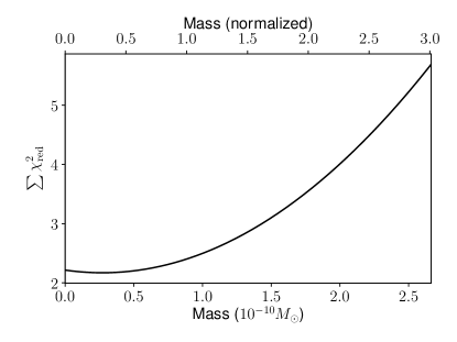
Figure 1: Results of the mass marching algorithm applied to synthetic data. The sum of the $\chi^{2}_{\mathrm{red}}$ values for both asteroids is shown on the $y$-axis. The bottom $x$-axis represents perturber mass in solar mass $\,\mathrm{M}_{\odot}$, while the top $x$-axis is normalized such that 1 represents the correct mass, 2 is twice that, etc.

Residuals corresponding to the best-fit solution are shown in Fig. 2. They are very small, which is expected, since the synthetic data was generated with very small errors. Residuals are noticeably higher for the test asteroid than for the perturber, which is expected as the test asteroid’s astrometry had errors approximately 5 times larger than those of the perturber. Interestingly, there appears to be a slight linear trend in the right ascension residuals, where they appear to slightly decrease with time in a linear trend. This is caused by a too small semi-major axis leading to a too large mean motion and, further, systematic decrease of the $O-C$ residual in RA.

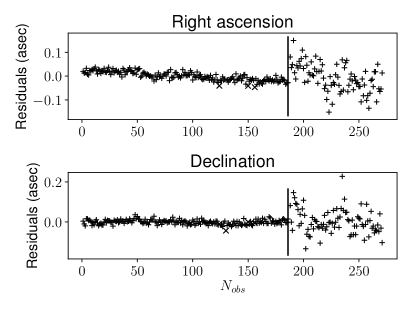
Figure 2: Residuals of the best fit for synthetic data obtained with the mass marching method. The data for the perturber and the test asteroid are separated by the vertical line, with the perturber’s data on the left side. The data points are sorted by observation time in such a manner that each asteroid’s data begins with the earliest observation and ends with the last.

We also ran the marching algorithm for all real encounters considered. Similarly to the synthetic case, we determined the initial orbits with least-squares. In the case of [19;3486], the marching algorithm finds a non-zero best fit mass that is approximately 75% of the mass from Carry (2012), which is actually a very good result considering the approximations used (Fig. 3).

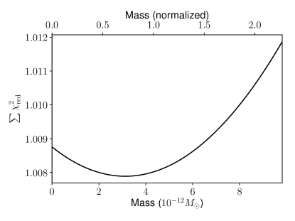
Figure 3: Results of the mass marching algorithm applied to the [19;3486] encounter. The sum of the $\chi^{2}_{\mathrm{red}}$ values for both asteroids is shown on the $y$-axis. The bottom $x$-axis represents perturber mass in solar mass $\,\mathrm{M}_{\odot}$, while the top $x$-axis is normalized such that 1 represents the mass from Carry (2012), 2 is twice that, etc.

The case of [15;14401], however, is an example of a problematic case for the marching algorithm in that the algorithm finds a best-fit mass of zero (Fig. 4).

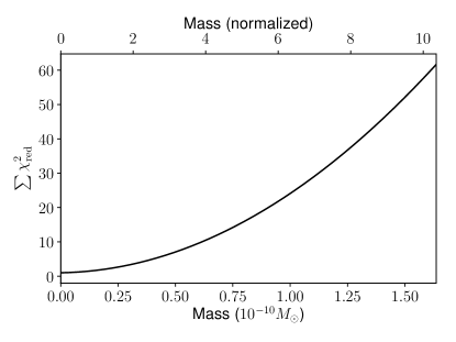
Figure 4: Results of the mass marching algorithm applied to the [15;14401] encounter.

To verify that the method performs correctly in a case where zero mass is expected, we ran the marching algorithm for an arbitrary pair of asteroids, [14328;4665], that do not experience a close encounter. This being the case, it logically follows that perturber mass should have no effect on the $\chi^{2}$ value. This is exactly the result we see in Fig. 5.

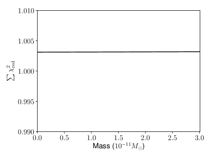
Figure 5: Results of the mass marching algorithm applied to [14328;4665].

Taken together, the above results imply that a correlation between the mass of the perturber and $\chi^{2}$ indicates that the close encounters has potential for useful mass estimation, even when the best-fit mass is zero.

The best-fit masses for all cases can be seen in Table 3. The best-fit mass is zero in four cases (all show a correlation between mass and $\chi^{2}$), while the other five give results fairly similar to literature values.

Table 3: Compilation of the marching algorithm’s results for all used encounters. The reference masses are from Carry (2012).

Encounter	Marching result	Ref. mass
	[$10^{-11}\,\mathrm{M}_{\odot}$]	[$10^{-11}\,\mathrm{M}_{\odot}$]
[7;17186]	$0.120$	$0.649\pm 0.106$
[10;3946]	$2.02$	$4.34\pm 0.26$
[13;14689]	$0.00$	$0.444\pm 0.214$
[15;14401]	$0.00$	$1.58\pm 0.09$
[19;3486]	$0.307$	$0.433\pm 0.073$
[19;27799]	$0.307$	$0.433\pm 0.073$
[29;987]	$0.00$	$0.649\pm 0.101$
[52;124]	$1.45$	$1.20\pm 0.29$
[704;7461]	$0.00$	$1.65\pm 0.23$

Given the nature of the marching algorithm, it is logical that the zero mass for [15;14401] resulted from inaccurate initial orbits, which did not take the perturbating asteroid’s non-zero mass into account. To verify this explanation, we calculated two separate initial orbits. The first used pre-encounter astrometry only and the second used post-encounter astrometry only. We then ran the marching algorithm separately for both orbits while using all of our available astrometry. Both of these initial orbits result in a non-zero minimum (Fig. 6) unlike the initial orbit that used all of our astrometry. This confirms that the zero minimum was indeed caused by inaccurate initial orbits. In addition, the curves have very similar shapes, although the $\chi^{2}_{\mathrm{red}}$ values are quite different.

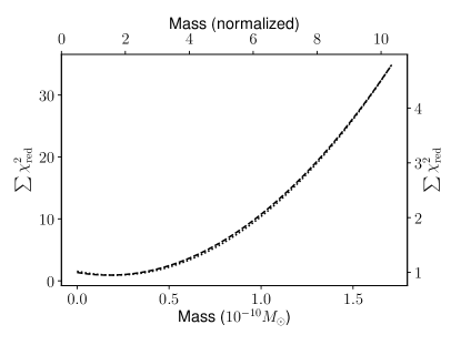
Figure 6: Results of the mass marching algorithm applied to the [15;14401] encounter using two separate initial orbits calculated with pre- and post-encounter astrometry respectively. The dashed line and the left y-axis correspond to the pre-encounter orbit while the dotted line and the right y-axis correspond to the post-encounter orbit.

4.2 Results for the Nelder-Mead algorithm

The Nelder-Mead algorithm fits for both the best mass and orbital elements. We first ran the Nelder-Mead algorithm for the synthetic data. The best fit mass found was $6.94\times 10^{-11}\,\mathrm{M}_{\odot}$, which is slightly lower than the marching result and, in this case, approximately 78% of the correct value, which is a reasonable result. As one would expect, the fit is significantly better than that of the marching algorithm, as the marching algorithm’s best $\chi^{2}_{\mathrm{red}}$ value is 2.17, while the best Nelder-Mead fit had a $\chi^{2}_{\mathrm{red}}$ value of 1.16.

Residuals for the Nelder-Mead method are shown in Fig. 7. The residuals still appear reasonable, and in comparison to the marching residuals shown in Fig. 2, the Nelder-Mead residuals are clearly lower and the systematic trend in the right ascension is gone due to the algorithm improving the used orbits themselves. For comparison, the test asteroid’s RMS values from the best fit of the marching algorithm were 0.058" and 0.061" for the right ascension and declination respectively while the equivalent values from the Nelder-Mead run were 0.044" and 0.052", which are clearly lower values and thus a better fit.

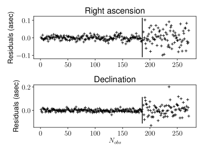
Figure 7: Residuals of the best fit for synthetic data obtained with the Nelder-Mead method. The data for the perturber and the test asteroid are separated by the vertical line, with the perturber’s data on the left side. The data points are sorted by observation time in such a manner that each asteroid’s data begins with the earliest observation and ends with the last.

Results for the real encounters can be seen in Table 4. In most cases, the result is again similar to literature values. Notable exceptions include [13;14689], [29;987], in which the result is too large, and [52;124], where it is too small. Of course, one has to keep in mind that these estimates do not include uncertainties.

Table 4: Compilation of the Nelder-Mead algorithm’s results for the real encounters considered. The reference masses are from Carry (2012).

Encounter	Nelder-Mead result	Ref. mass
	[$10^{-11}\,\mathrm{M}_{\odot}$]	[$10^{-11}\,\mathrm{M}_{\odot}$]
[7;17186]	0.503	$0.649\pm 0.106$
[10;3946]	2.76	$4.34\pm 0.26$
[13;14689]	1.37	$0.444\pm 0.214$
[15;14401]	3.29	$1.58\pm 0.09$
[19;3486]	0.232	$0.433\pm 0.073$
[19;27799]	0.220	$0.433\pm 0.073$
[29;987]	1.43	$0.649\pm 0.101$
[52;124]	0.774	$1.20\pm 0.29$
[704;7461]	2.98	$1.65\pm 0.23$

4.3 MCMC algorithm results

We ran the MCMC algorithm for both the synthetic case and all of the real encounters considered for a total of 50,000 transitions. Fig. 8 displays the resulting probability distribution of perturber mass for the synthetic test case. Upon examination of the kernel density estimate, which estimates the probability density function of the mass, one can see that the best fitting mass is approximately $6.71\times 10^{-11}\,\mathrm{M}_{\odot}$, or 76% of the correct mass of $8.85\times 10^{-11}\,\mathrm{M}_{\odot}$. Interestingly, the result is very close to our Nelder-Mead results. The correct result is within our $3\sigma$ confidence limits. It is also apparent that the probability distribution in this case is essentially Gaussian.

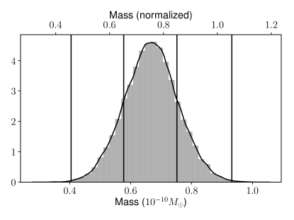
Figure 8: A histogram of masses for all transitions of the MCMC chain for synthetic data. Each mass is weighted by the total amount of repetitions for that particular transition, i.e., if a set of parameters is accepted $n$ times in a row, it will be counted $n$ times into the histogram. The bottom $x$ axis represents mass in solar mass $\,\mathrm{M}_{\odot}$, while the top $x$ axis is normalized such that 1.0 represents the correct mass. The black graph represents a kernel density estimate while the vertical lines represent the $1\sigma$ and $3\sigma$ confidence limits. The $y$ axis is normalized such that the kernel density estimate’s integral over the whole $x$ axis is one.

For comparison, we have also included a logarithmic scatter plot of mass versus the probability density value for each transition (Fig. 9). It is apparent that the scatter plot matches the distribution quite well, and one can also see that the distributions for both halves of the chain are quite similar. These result are to be expected, and shows that there appear to be no major issues with the chain itself.

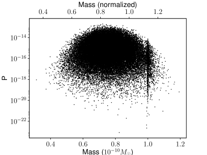
Figure 9: Scatter plot of mass versus probability density value for all transitions of the MCMC chain for synthetic data. The vertical clump of data points at roughly $10^{-10}\,\mathrm{M}_{\odot}$ corresponds to the initial burn-in phase where the proposal distribution is far too narrow.

Figures 10 and 11 display the trace of the orbital elements for both the perturbing asteroid and the test asteroid. The algorithm converges very fast, with no visible burn-in period on this scale, and there are no mixing issues to be seen. Overall the figures look exactly like what one would expect from a good MCMC chain.

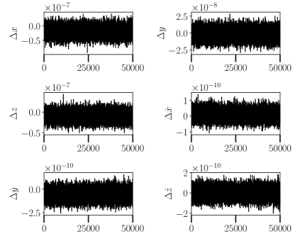
Figure 10: The trace of the MCMC chain in terms of perturber orbital elements when using the synthetic astrometry. The $x$-axis displays the number of the transition, while the $y$-axis represents difference from the initial orbit.The units are in au and au/day.

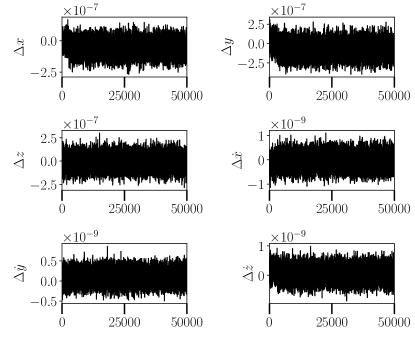
Figure 11: The trace of the MCMC chain in terms of test asteroid orbital elements in the synthetic case. The $x$-axis displays the number of the transition, while the $y$-axis represents difference from the initial orbit. The units are in au and au/day.

To showcase the usefulness of AM, we have included equivalent plots showing the evolution of each orbital element in the synthetic test case without AM in Figs 12 and 13. Upon visual examination it is immediately apparent that mixing is poor in all cases, and $z$ of the perturber and $\dot{z}$ of the test asteroid do not converge properly. When compared with the equivalent Figs. 10 and 11 where AM was used, the difference is substantial. It is clear that AM by itself has completely negated these problems and thus greatly improved our algorithm.

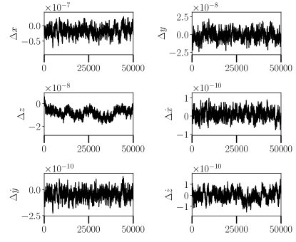
Figure 12: The trace of the MCMC chain in terms of perturber orbital elements for a run without Adaptive Metropolis using the synthetic astrometry. There are visible convergence and mixing issues due to poor initial proposal distributions. The $x$-axis displays the number of the transition, while the $y$-axis represents difference from the initial orbit. The units are in au and au/day.

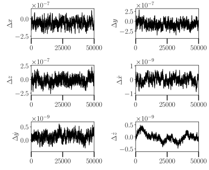
Figure 13: The trace of the MCMC chain in terms of test asteroid orbital elements for a run without Adaptive Metropolis using the synthetic astrometry. There are visible convergence and mixing issues due to poor initial proposal distributions. The $x$-axis displays the number of the transition, while the $y$-axis represents difference from the initial orbit. The units are in au and au/day.

Finally, Figs. 14 and 15 show the distributions of the orbital elements for both the perturber and test asteroid in the case of synthetic astrometry. The distributions also appear to be largely Gaussian and quite narrow.

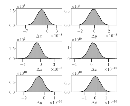
Figure 14: Histograms of the Cartesian state vectors for the perturber for all transitions of the MCMC chain for synthetic data. Each element is weighted by the total amount of repetitions for that particular transition, i.e. if a proposal is accepted $n$ times in a row, it will be counted $n$ times into the histogram. The bottom $x$ axis represents difference between the initial synthetic orbit and the tested orbit, which means that 0.0 corresponds to the initial orbit. The units are in au and au/day. The black graph represents a kernel density estimate while the $y$ axis is normalized such that the kernel density estimate’s integral over the whole $x$ axis is one.

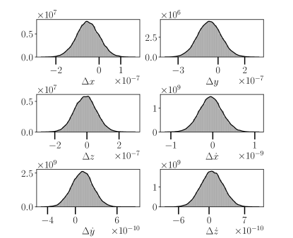
Figure 15: Histograms of Cartesian state vectors for the test asteroid for all transitions of the MCMC chain for synthetic data. Each element is weighted by the total amount of repetitions for that particular proposal, i.e. if a proposal is accepted $n$ times in a row, it will be counted $n$ times into the histogram. The bottom $x$ axis represents difference between the initial synthetic orbit and the tested orbit, which means that 0.0 corresponds to the initial orbit. The units are in au and au/day. The black graph represents a kernel density estimate while the $y$ axis is normalized such that the kernel density estimate’s integral over the whole $x$ axis is one.

Example results for real asteroids are shown in Fig. 16. The figure shows the resulting mass probability distributions for the [19;3486] and [19;27799] encounters. Note that in both cases, the perturbing asteroid is the same, and thus the correct mass should also be the same. However, the choice of the test asteroid has a significant impact on the results due to observational errors and systematic biases. Such a result is not unprecedented: for instance Baer et al. (2011) obtained a value of $(3.90\pm 0.37)\times 10^{-12}\,\mathrm{M}_{\odot}$ for [19;3486] and $(9.10\pm 1.6)\times 10^{-12}\,\mathrm{M}_{\odot}$ for [19;27799], a roughly 2x difference. The value of Carry (2012) is a weighted average of all mass estimates for this asteroid and as such, is not dependent on only a single test asteroid.

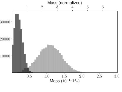
Figure 16: Results of the MCMC algorithm applied to the [19;3486] (darker shade) and [19;27799] encounters. The upper x-axis is normalized such that 1.0 equals the literature value of Carry (2012).

One can see that our maximum-likelihood solutions for either pair do not perfectly correspond to the literature value of Carry (2012), but it remains well within the 3-sigma limits of both. Intriguingly, the literature value for the mass corresponds well to the peak of the area where both histograms overlap. This suggests that if we were to use both test asteroids simultaneously, we would get results much closer to the literature value. This is encouraging, as we intend to extend our algorithm to use multiple test asteroids and/or perturbers simultaneously. The Nelder-Mead algorithm found masses of $2.32\times 10^{-12}\,\mathrm{M}_{\odot}$ and $2.20\times 10^{-12}\,\mathrm{M}_{\odot}$ for these encounters respectively, which intriguingly are much closer to each other than the MCMC results.

Figure 17 shows a case where the probability distribution of perturber mass is clearly non-Gaussian, thus showing that Gaussian error estimates are incorrect for this case. Again our maximum-likelihood mass does not correspond to the literature value, but is still well within uncertainty limits.

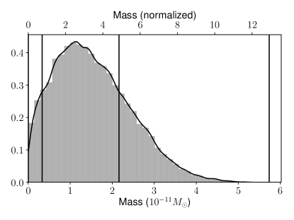
Figure 17: Results of the MCMC algorithm applied to the [13;14689] encounter. The upper x-axis is normalized such that 1.0 equals the literature value of Carry (2012).

[13;14689] is also the only case where AM had a significant impact on the mass probability distribution. For comparison, the equivalent plot of a run of the same length without AM is shown in Fig. 18. Clearly, in this case mass does not converge properly, likely due to poor convergence and mixing of the orbits. In our other cases, the impact of AM on perturber mass was much smaller despite the significant improvement on mixing and convergence of the orbital elements.

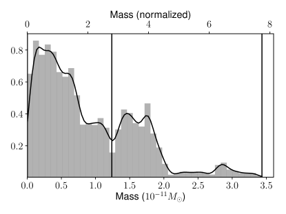
Figure 18: Results of the MCMC algorithm without Adaptive Metropolis applied to the [13;14689] encounter. The upper x-axis is normalized such that 1.0 equals the literature value of Carry (2012).

Table 5: Compilation of the MCMC algorithm’s results for all used encounters. The reference masses are from Carry (2012).

Encounter	ML mass	$1\sigma$ boundaries	$3\sigma$ boundaries	Ref. mass
	[$10^{-11}\,\mathrm{M}_{\odot}$]	[$10^{-11}\,\mathrm{M}_{\odot}$]	[$10^{-11}\,\mathrm{M}_{\odot}$]	[$10^{-11}\,\mathrm{M}_{\odot}$]
Synthetic	6.71	[5.84, 7.62]	[4.09, 9.43]	8.85 $\pm$ 0.00
[7;17186]	0.210	[0.0499, 0.354]	[0.000660, 1.20]	0.649 $\pm$ 0.106
[10;3946]	2.48	[2.21, 2.77]	[1.63, 3.32]	4.34 $\pm$ 0.26
[13;14689]	1.13	[0.332, 2.16]	[0.00273, 5.74]	0.444 $\pm$ 0.214
[15;14401]	1.11	[0.914, 1.25]	[0.574, 1.61]	1.58 $\pm$ 0.09
[19;3486]	0.141	[0.0567, 0.285]	[0.000467, 0.828]	0.433 $\pm$ 0.073
[19;27799]	1.11	[0.757, 1.42]	[0.122, 2.05]	0.44 $\pm$ 0.073
[29;987]	0.258	[0.0163, 0.898]	[0.00238, 4.43]	0.649 $\pm$ 0.101
[52;124]	0.893	[0.232, 1.91]	[0.00319, 6.05]	1.20 $\pm$ 0.29
[704;7461]	0.155	[0.00910, 0.664]	[0.00182, 3.50]	1.65 $\pm$ 0.23

Table 5 shows our MCMC results for all of our selected encounters along with their uncertainty limits. One can see that in almost all cases, our maximum-likelihood results do not perfectly correspond to the weighted average values of Carry (2012). Nonetheless, in almost all cases the literature values are well within our $3\sigma$ confidence limits and within $1\sigma$ in several cases. These confidence limits are also quite wide in comparison to those in literature and, significantly, in many cases non-Gaussian. This can be seen by examining the uncertainty limits: for Gaussian probability distributions, the $3\sigma$ uncertainty limits should be three times higher than the equivalent $1\sigma$ limits. As an example, in the case of [704;7461] the upper $3\sigma$ limit is in fact approximately 4 times the $1\sigma$ limit, which means that the distribution here has a longer tail than a Gaussian distribution would. On the other hand, the difference between the lower limits is tiny and also clearly non-Gaussian. The Gaussian cases of the synthetic pair, [15;14401], and [10;3946] interestingly have notably smaller confidence limits than the other cases. This suggests that the symmetric confidence limits typically used in literature are actually very inaccurate in non-Gaussian cases.

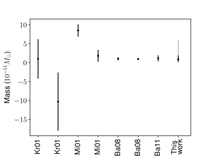
Figure 19: A comparison of our results and previous mass estimates (Krasinsky et al., 2001; Michalak, 2001; Baer and Chesley, 2008; Baer et al., 2011) for (52) Eunomia done with the close encounter method. Only previous estimates computed with a single test asteroid are shown. When results for multiple test asteroids had been reported separately, we selected the maximum and minimum values. The rightmost data point represents our results, where the black error bars represent the $1\sigma$ uncertainty limit while the gray error bar represents the $3\sigma$ limit.

Figure 19 shows how our results for (52) Europa compare to previous mass estimates for this asteroid. Interestingly, while the earlier estimates of this case largely disagree with each other, apart from the negative value every single one of these estimates falls within our 3$\sigma$ uncertainty limits. This appears to confirm that previous uncertainties are indeed far too small, and that our MCMC algorithm provides more realistic uncertainty estimates. One can also see here that the upper $3\sigma$ limit is significantly larger than the Gaussian limit would be, which shows that probability distribution also is not Gaussian in this case. The wide uncertainty estimates may also in part be explained by the limited amount of pre-encounter astrometry used. Nonetheless, our result remains within 1$\sigma$ of the Carry (2012) value. An equivalent plot for (15) Eunomia is shown in Figure 20. These results appear closer to, but not quite, Gaussian.

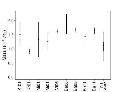
Figure 20: A comparison of our results and previous mass estimates (Krasinsky et al., 2001; Michalak, 2001; Vitagliano and Stoss, 2006; Baer and Chesley, 2008; Baer et al., 2011) for (15) Eunomia done with the close encounter method. Only previous estimates computed with a single test asteroid are shown. When results for multiple test asteroids had been reported separately, we selected the maximum and minimum values. The rightmost data point represents our results, where the black error bars represent the $1\sigma$ uncertainty limit while the gray error bar represents the $3\sigma$ limit.

In most cases, the MCMC results are fairly similar to those of the Nelder-Mead algorithm (Table 4) with some exceptions, such as [704;7461] where Nelder-Mead is very close to the literature value unlike the MCMC algorithm. Conversely, in some other cases such as [13;14689] the MCMC result is much better. Overall, the results for both algorithms are in line with each other.

5 Conclusions

We have successfully developed and implemented a new Adaptive-Metropolis algorithm for asteroid mass estimation. Our results agree with previously published mass estimates, but suggest that the published uncertainties may be misleading as a consequence of using linearized mass-estimation methods. Future work on the methodology includes extending the algorithm to use multiple perturbers and/or test asteroids simultaneously, more robust observational error and outlier rejection models, and accounting for systematic errors automatically. Finally, we intend to expand the application of the method by systematically obtaining mass estimates using existing astrometry and, eventually, from the Gaia mission once the data is released.

References

References

- Baer and Chesley (2008) Baer, J. and Chesley, S. R. (2008). Astrometric masses of 21 asteroids, and an integrated asteroid ephemeris. Celestial Mechanics and Dynamical Astronomy, 100:27–42.
- Baer et al. (2011) Baer, J., Chesley, S. R., and Matson, R. D. (2011). Astrometric Masses of 26 Asteroids and Observations on Asteroid Porosity. AJ, 141:143.
- Carry (2012) Carry, B. (2012). Density of asteroids. Planet. Space Sci., 73:98–118.
- Chesley et al. (2002) Chesley, S. R., Chodas, P. W., Milani, A., Valsecchi, G. B., and Yeomans, D. K. (2002). Quantifying the risk posed by potential earth impacts. Icarus, 159(2):423 – 432.
- DeMeo and Carry (2014) DeMeo, F. E. and Carry, B. (2014). Solar System evolution from compositional mapping of the asteroid belt. Nature, 505:629–634.
- Feigelson and Babu (2012) Feigelson, E. D. and Babu, G. J. (2012). Modern Statistical Methods for Astronomy.
- Gaia Collaboration et al. (2016) Gaia Collaboration, Prusti, T., de Bruijne, J. H. J., Brown, A. G. A., Vallenari, A., Babusiaux, C., Bailer-Jones, C. A. L., Bastian, U., Biermann, M., Evans, D. W., Eyer, L., Jansen, F., Jordi, C., Klioner, S. A., Lammers, U., Lindegren, L., Luri, X., Mignard, F., Milligan, D. J., Panem, C., Poinsignon, V., Pourbaix, D., Randich, S., Sarri, G., Sartoretti, P., Siddiqui, H. I., Soubiran, C., Valette, V., van Leeuwen, F., Walton, N. A., Aerts, C., Arenou, F., Cropper, M., Drimmel, R., Høg, E., Katz, D., Lattanzi, M. G., O’Mullane, W., Grebel, E. K., Holland, A. D., Huc, C., Passot, X., Bramante, L., Cacciari, C., Castañeda, J., Chaoul, L., Cheek, N., De Angeli, F., Fabricius, C., Guerra, R., Hernández, J., Jean-Antoine-Piccolo, A., Masana, E., Messineo, R., Mowlavi, N., Nienartowicz, K., Ordóñez-Blanco, D., Panuzzo, P., Portell, J., Richards, P. J., Riello, M., Seabroke, G. M., Tanga, P., Thévenin, F., Torra, J., Els, S. G., Gracia-Abril, G., Comoretto, G., Garcia-Reinaldos, M., Lock, T., Mercier, E., Altmann, M., Andrae, R., Astraatmadja, T. L., Bellas-Velidis, I., Benson, K., Berthier, J., Blomme, R., Busso, G., Carry, B., Cellino, A., Clementini, G., Cowell, S., Creevey, O., Cuypers, J., Davidson, M., De Ridder, J., de Torres, A., Delchambre, L., Dell’Oro, A., Ducourant, C., Frémat, Y., García-Torres, M., Gosset, E., Halbwachs, J.-L., Hambly, N. C., Harrison, D. L., Hauser, M., Hestroffer, D., Hodgkin, S. T., Huckle, H. E., Hutton, A., Jasniewicz, G., Jordan, S., Kontizas, M., Korn, A. J., Lanzafame, A. C., Manteiga, M., Moitinho, A., Muinonen, K., Osinde, J., Pancino, E., Pauwels, T., Petit, J.-M., Recio-Blanco, A., Robin, A. C., Sarro, L. M., Siopis, C., Smith, M., Smith, K. W., Sozzetti, A., Thuillot, W., van Reeven, W., Viala, Y., Abbas, U., Abreu Aramburu, A., Accart, S., Aguado, J. J., Allan, P. M., Allasia, W., Altavilla, G., Álvarez, M. A., Alves, J., Anderson, R. I., Andrei, A. H., Anglada Varela, E., Antiche, E., Antoja, T., Antón, S., Arcay, B., Atzei, A., Ayache, L., Bach, N., Baker, S. G., Balaguer-Núñez, L., Barache, C., Barata, C., Barbier, A., Barblan, F., Baroni, M., Barrado y Navascués, D., Barros, M., Barstow, M. A., Becciani, U., Bellazzini, M., Bellei, G., Bello García, A., Belokurov, V., Bendjoya, P., Berihuete, A., Bianchi, L., Bienaymé, O., Billebaud, F., Blagorodnova, N., Blanco-Cuaresma, S., Boch, T., Bombrun, A., Borrachero, R., Bouquillon, S., Bourda, G., Bouy, H., Bragaglia, A., Breddels, M. A., Brouillet, N., Brüsemeister, T., Bucciarelli, B., Budnik, F., Burgess, P., Burgon, R., Burlacu, A., Busonero, D., Buzzi, R., Caffau, E., Cambras, J., Campbell, H., Cancelliere, R., Cantat-Gaudin, T., Carlucci, T., Carrasco, J. M., Castellani, M., Charlot, P., Charnas, J., Charvet, P., Chassat, F., Chiavassa, A., Clotet, M., Cocozza, G., Collins, R. S., Collins, P., Costigan, G., Crifo, F., Cross, N. J. G., Crosta, M., Crowley, C., Dafonte, C., Damerdji, Y., Dapergolas, A., David, P., David, M., De Cat, P., de Felice, F., de Laverny, P., De Luise, F., De March, R., de Martino, D., de Souza, R., Debosscher, J., del Pozo, E., Delbo, M., Delgado, A., Delgado, H. E., di Marco, F., Di Matteo, P., Diakite, S., Distefano, E., Dolding, C., Dos Anjos, S., Drazinos, P., Durán, J., Dzigan, Y., Ecale, E., Edvardsson, B., Enke, H., Erdmann, M., Escolar, D., Espina, M., Evans, N. W., Eynard Bontemps, G., Fabre, C., Fabrizio, M., Faigler, S., Falcão, A. J., Farràs Casas, M., Faye, F., Federici, L., Fedorets, G., Fernández-Hernández, J., Fernique, P., Fienga, A., Figueras, F., Filippi, F., Findeisen, K., Fonti, A., Fouesneau, M., Fraile, E., Fraser, M., Fuchs, J., Furnell, R., Gai, M., Galleti, S., Galluccio, L., Garabato, D., García-Sedano, F., Garé, P., Garofalo, A., Garralda, N., Gavras, P., Gerssen, J., Geyer, R., Gilmore, G., Girona, S., Giuffrida, G., Gomes, M., González-Marcos, A., González-Núñez, J., González-Vidal, J. J., Granvik, M., Guerrier, A., Guillout, P., Guiraud, J., Gúrpide, A., Gutiérrez-Sánchez, R., Guy, L. P., Haigron, R., Hatzidimitriou, D., Haywood, M., Heiter, U., Helmi, A., Hobbs, D., Hofmann, W., Holl, B., Holland, G., Hunt, J. A. S., Hypki, A., Icardi, V., Irwin, M., Jevardat de Fombelle, G., Jofré, P., Jonker, P. G., Jorissen, A., Julbe, F., Karampelas, A., Kochoska, A., Kohley, R., Kolenberg, K., Kontizas, E., Koposov, S. E., Kordopatis, G., Koubsky, P., Kowalczyk, A., Krone-Martins, A., Kudryashova, M., Kull, I., Bachchan, R. K., Lacoste-Seris, F., Lanza, A. F., Lavigne, J.-B., Le Poncin-Lafitte, C., Lebreton, Y., Lebzelter, T., Leccia, S., Leclerc, N., Lecoeur-Taibi, I., Lemaitre, V., Lenhardt, H., Leroux, F., Liao, S., Licata, E., Lindstrøm, H. E. P., Lister, T. A., Livanou, E., Lobel, A., Löffler, W., López, M., Lopez-Lozano, A., Lorenz, D., Loureiro, T., MacDonald, I., Magalhães Fernandes, T., Managau, S., Mann, R. G., Mantelet, G., Marchal, O., Marchant, J. M., Marconi, M., Marie, J., Marinoni, S., Marrese, P. M., Marschalkó, G., Marshall, D. J., Martín-Fleitas, J. M., Martino, M., Mary, N., Matijevič, G., Mazeh, T., McMillan, P. J., Messina, S., Mestre, A., Michalik, D., Millar, N. R., Miranda, B. M. H., Molina, D., Molinaro, R., Molinaro, M., Molnár, L., Moniez, M., Montegriffo, P., Monteiro, D., Mor, R., Mora, A., Morbidelli, R., Morel, T., Morgenthaler, S., Morley, T., Morris, D., Mulone, A. F., Muraveva, T., Musella, I., Narbonne, J., Nelemans, G., Nicastro, L., Noval, L., Ordénovic, C., Ordieres-Meré, J., Osborne, P., Pagani, C., Pagano, I., Pailler, F., Palacin, H., Palaversa, L., Parsons, P., Paulsen, T., Pecoraro, M., Pedrosa, R., Pentikäinen, H., Pereira, J., Pichon, B., Piersimoni, A. M., Pineau, F.-X., Plachy, E., Plum, G., Poujoulet, E., Prša, A., Pulone, L., Ragaini, S., Rago, S., Rambaux, N., Ramos-Lerate, M., Ranalli, P., Rauw, G., Read, A., Regibo, S., Renk, F., Reylé, C., Ribeiro, R. A., Rimoldini, L., Ripepi, V., Riva, A., Rixon, G., Roelens, M., Romero-Gómez, M., Rowell, N., Royer, F., Rudolph, A., Ruiz-Dern, L., Sadowski, G., Sagristà Sellés, T., Sahlmann, J., Salgado, J., Salguero, E., Sarasso, M., Savietto, H., Schnorhk, A., Schultheis, M., Sciacca, E., Segol, M., Segovia, J. C., Segransan, D., Serpell, E., Shih, I-C., Smareglia, R., Smart, R. L., Smith, C., Solano, E., Solitro, F., Sordo, R., Soria Nieto, S., Souchay, J., Spagna, A., Spoto, F., Stampa, U., Steele, I. A., Steidelmüller, H., Stephenson, C. A., Stoev, H., Suess, F. F., Süveges, M., Surdej, J., Szabados, L., Szegedi-Elek, E., Tapiador, D., Taris, F., Tauran, G., Taylor, M. B., Teixeira, R., Terrett, D., Tingley, B., Trager, S. C., Turon, C., Ulla, A., Utrilla, E., Valentini, G., van Elteren, A., Van Hemelryck, E., van Leeuwen, M., Varadi, M., Vecchiato, A., Veljanoski, J., Via, T., Vicente, D., Vogt, S., Voss, H., Votruba, V., Voutsinas, S., Walmsley, G., Weiler, M., Weingrill, K., Werner, D., Wevers, T., Whitehead, G., Wyrzykowski, Ł., Yoldas, A., Žerjal, M., Zucker, S., Zurbach, C., Zwitter, T., Alecu, A., Allen, M., Allende Prieto, C., Amorim, A., Anglada-Escudé, G., Arsenijevic, V., Azaz, S., Balm, P., Beck, M., Bernstein, H.-H., Bigot, L., Bijaoui, A., Blasco, C., Bonfigli, M., Bono, G., Boudreault, S., Bressan, A., Brown, S., Brunet, P.-M., Bunclark, P., Buonanno, R., Butkevich, A. G., Carret, C., Carrion, C., Chemin, L., Chéreau, F., Corcione, L., Darmigny, E., de Boer, K. S., de Teodoro, P., de Zeeuw, P. T., Delle Luche, C., Domingues, C. D., Dubath, P., Fodor, F., Frézouls, B., Fries, A., Fustes, D., Fyfe, D., Gallardo, E., Gallegos, J., Gardiol, D., Gebran, M., Gomboc, A., Gómez, A., Grux, E., Gueguen, A., Heyrovsky, A., Hoar, J., Iannicola, G., Isasi Parache, Y., Janotto, A.-M., Joliet, E., Jonckheere, A., Keil, R., Kim, D.-W., Klagyivik, P., Klar, J., Knude, J., Kochukhov, O., Kolka, I., Kos, J., Kutka, A., Lainey, V., LeBouquin, D., Liu, C., Loreggia, D., Makarov, V. V., Marseille, M. G., Martayan, C., Martinez-Rubi, O., Massart, B., Meynadier, F., Mignot, S., Munari, U., Nguyen, A.-T., Nordlander, T., Ocvirk, P., O’Flaherty, K. S., Olias Sanz, A., Ortiz, P., Osorio, J., Oszkiewicz, D., Ouzounis, A., Palmer, M., Park, P., Pasquato, E., Peltzer, C., Peralta, J., Péturaud, F., Pieniluoma, T., Pigozzi, E., Poels, J., Prat, G., Prod’homme, T., Raison, F., Rebordao, J. M., Risquez, D., Rocca-Volmerange, B., Rosen, S., Ruiz-Fuertes, M. I., Russo, F., Sembay, S., Serraller Vizcaino, I., Short, A., Siebert, A., Silva, H., Sinachopoulos, D., Slezak, E., Soffel, M., Sosnowska, D., Straižys, V., ter Linden, M., Terrell, D., Theil, S., Tiede, C., Troisi, L., Tsalmantza, P., Tur, D., Vaccari, M., Vachier, F., Valles, P., Van Hamme, W., Veltz, L., Virtanen, J., Wallut, J.-M., Wichmann, R., Wilkinson, M. I., Ziaeepour, H., and Zschocke, S. (2016). The gaia mission. A&A, 595:A1.
- Galád and Gray (2002) Galád, A. and Gray, B. (2002). Asteroid encounters suitable for mass determinations. A&A, 391:1115–1122.
- Granvik et al. (2009) Granvik, M., Virtanen, J., Oszkiewicz, D., and Muinonen, K. (2009). OpenOrb: Open-source asteroid orbit computation software including statistical ranging. Meteoritics and Planetary Science, 44:1853–1861.
- Haario et al. (2001) Haario, H., Saksman, E., and Tamminen, J. (2001). An adaptive metropolis algorithm. Bernoulli, 7(2):223–242.
- Hertz (1966) Hertz, H. G. (1966). The Mass of Vesta. IAU Circ., 1983:3.
- Hilton (2002) Hilton, J. L. (2002). Asteroid Masses and Densities. Asteroids III, pages 103–112.
- Krasinsky et al. (2001) Krasinsky, G. A., Pitjeva, E. V., Vasiliev, M. V., and Yagudina, E. I. (2001). Estimating masses of asteroids. In Communications of IAA of RAS.
- Michalak (2001) Michalak, G. (2001). Determination of asteroid masses. II. (6) Hebe, (10) Hygiea, (15) Eunomia, (52) Europa, (88) Thisbe, (444) Gyptis, (511) Davida and (704) Interamnia. A&A, 374:703–711.
- Mouret et al. (2008) Mouret, S., Hestroffer, D., and Mignard, F. (2008). Asteroid mass determination with the Gaia mission. A simulation of the expected precisions. Planet. Space Sci., 56:1819–1822.
- Nelder and Mead (1965) Nelder, J. A. and Mead, R. (1965). A simplex method for function minimization. Computer Journal, 7:308–313.
- Petit et al. (1997) Petit, J.-M., Durda, D. D., Greenberg, R., Hurford, T. A., and Geissler, P. E. (1997). The Long-Term Dynamics of Dactyl’s Orbit. Icarus, 130:177–197.
- Russell et al. (2016) Russell, C. T., Raymond, C. A., Ammannito, E., Buczkowski, D. L., De Sanctis, M. C., Hiesinger, H., Jaumann, R., Konopliv, A. S., McSween, H. Y., Nathues, A., Park, R. S., Pieters, C. M., Prettyman, T. H., McCord, T. B., McFadden, L. A., Mottola, S., Zuber, M. T., Joy, S. P., Polanskey, C., Rayman, M. D., Castillo-Rogez, J. C., Chi, P. J., Combe, J. P., Ermakov, A., Fu, R. R., Hoffmann, M., Jia, Y. D., King, S. D., Lawrence, D. J., Li, J.-Y., Marchi, S., Preusker, F., Roatsch, T., Ruesch, O., Schenk, P., Villarreal, M. N., and Yamashita, N. (2016). Dawn arrives at Ceres: Exploration of a small, volatile-rich world. Science, 353:1008–1010.
- Russell et al. (2012) Russell, C. T., Raymond, C. A., Coradini, A., McSween, H. Y., Zuber, M. T., Nathues, A., De Sanctis, M. C., Jaumann, R., Konopliv, A. S., Preusker, F., Asmar, S. W., Park, R. S., Gaskell, R., Keller, H. U., Mottola, S., Roatsch, T., Scully, J. E. C., Smith, D. E., Tricarico, P., Toplis, M. J., Christensen, U. R., Feldman, W. C., Lawrence, D. J., McCoy, T. J., Prettyman, T. H., Reedy, R. C., Sykes, M. E., and Titus, T. N. (2012). Dawn at Vesta: Testing the Protoplanetary Paradigm. Science, 336:684.
- Scholl et al. (1987) Scholl, H., Schmadel, L. D., and Roser, S. (1987). The mass of the asteroid (10) Hygiea derived from observations of (829) Academia. A&A, 179:311–316.
- Schubart (1970) Schubart, J. (1970). The Mass of Ceres. IAU Circ., 2268:1.
- Schubart (1974) Schubart, J. (1974). The Masses of the First Two Asteroids. A&A, 30:289–292.
- Standish and Hellings (1989) Standish, E. M. and Hellings, R. W. (1989). A determination of the masses of Ceres, Pallas, and Vesta from their perturbations upon the orbit of Mars. Icarus, 80:326–333.
- Standish (2000) Standish, M. (2000). Dynamical Reference Frame - Current Relevance and Future Prospects. In Johnston, K. J., McCarthy, D. D., Luzum, B. J., and Kaplan, G. H., editors, IAU Colloq. 180: Towards Models and Constants for Sub-Microarcsecond Astrometry, page 120.
- Vitagliano and Stoss (2006) Vitagliano, A. and Stoss, R. M. (2006). New mass determination of (15) Eunomia based on a very close encounter with (50278) 2000CZ12. A&A, 455:L29–L31.
- Yeomans et al. (1997) Yeomans, D. K., Barriot, J.-P., Dunham, D. W., Farquhar, R. W., Giorgini, J. D., Helfrich, C. E., Konopliv, A. S., McAdams, J. V., Miller, J. K., Owen, Jr., W. M., Scheeres, D. J., Synnott, S. P., and Williams, B. G. (1997). Estimating the Mass of Asteroid 253 Mathilde from Tracking Data During the NEAR Flyby. Science, 278:2106.