Return to axi-symmetry for pipe flows generated after a fractal orifice.

Abstract

We present experimental results obtained from pipe flows generated by fractal shaped orifices or openings. We compare different fractal orifices and their efficiencies to re-generate axi-symmetric flows and to return to the standard flow generated by a perforated plate or a circular orifice plate. We consider two families of fractal openings: mono-orifice and complex-orifice and emphasize the differences between the two fractal families. For the Reynolds number we use, we found that there is an optimum iteration for the fractal level above which no improvement for practical application such as flowmetering is to be expected. The main parameters we propose for the characterisation of the fractal orifice are the connexity parameter, the symmetry angle and the gap to the wall $\delta^{*}_{g}$. The results presented here are among the firsts for flows forced through fractal openings and will serve as reference for future studies and bench marks for numerical applications.

Keywords: fractal turbulence, pipe flow, fractal orifice, orifice plate

1 Introduction

There have been early attempts at understanding turbulence using fractal formalism (Sreenivasan et al., 1989; Meneveau and Sreenivasan, 1990; Meneveau, 1991; Nicolleau, 1996), also by using wavelet analysis (Farge et al., 1993; Nicolleau and Vassilicos, 1999).

Experiments using fractal-generated turbulent flows have been developed more recently, these flows are based on geometrically complex, multi-scale shapes, following a fractal pattern. By contrast to classical turbulence where turbulence is generated using a grid made of regularly spaced bars or rods, fractal-generated turbulence relies on repeating a pattern at different scales and positions in the grid. Such flows seem to point towards different scalings and physics than the traditional Richardson-Kolmogorov cascade (for a more complete picture, see e.g. Mazellier and Vassilicos, 2010; Valente and Vassilicos, 2012).

In parallel to these new experimental approaches there have been more theoretical attempts at understanding how particular interactions would generate particular energy spectra (Michelitsch et al., 2009) but we are still far from any complete theory relating fractal and spectral aspects of turbulence.
The experimental results presented in this paper are different from other attempts (e.g. Seoud and Vassilicos, 2007) where the experiments were concerned with homogeneous isotropic turbulence. Here we concentrate on flow generated in a pipe. The flow is forced through a fractal opening and we study the effect of that opening on the velocity (mean and rms) profiles.
Our interest though still theoretical is also driven by applications. We are interested in the effect of a complex shape on the generation of turbulent flows in a pipe. The practical application is to use such shapes as optimal flowmeters or flow mixers. Studies of complex shaped orifice or lobed jets exist (e.g Nastase et al., 2011) here we concentrate on the effect of fractal iterations of a simple pattern.
Fractal shapes have been considered as an alternative to the classical circular orifice used for flowmetering. Fractal orifices have been shown to decrease pressure drops by as much as 10% when compared to the classical circular orifice (Abou-El-Azm et al., 2010; Nicolleau et al., 2011). They also improve the measurement quality when used as flowmeter conditioners (Manshoor et al., 2011). (See e.g. Nowakowski et al., 2011, for another type of non-conventional flowmeters.) A classical orifice flowmeter consists of a circular orifice which is placed in the pipe or duct to create a pressure drop. The flow rate is then deduced from this pressure drop. Behind the orifice a substantial pressure deficit occurs affecting the turbulence cascade process and slowing down the flow mixing which results in delaying the flow recovery and eventually in a net pressure loss.
Though the orifice plate as a differential flowmeter has gained an overwhelming popularity because of its low maintenance cost (no moving part) compared to many other existing flowmeters, its inherent inefficient flow mixing is a serious disadvange. Ideally we would like the flow to recover as fast as possible and as much as possible in order to lower the energy cost associated to the pressure drop necessary for flowmetering. By contrast, a classic perforated plate will give efficient flow mixing but no pressure drop significant enough for flowmetering applications.
Perhaps a forced (non-Kolmogorov) energy cascade could speed up the flow recovery by improving the flow mixing. This is where practical interest meets the theoretical research on fractal-generated turbulence which can provide interesting alternatives for forcing turbulence. To tackle this problem from the practical point of view, we developed fractal orifices, thought of as intermediary geometries in between circular orifice and classical perforated plates, and studied their performance as pressure drop generators.

2 Experimental Set-up

The wind tunnel and its experimental conditions have been reported in details in (Nicolleau et al., 2011), we just summarise them here. The schematic of the wind tunnel is shown in figure 1.

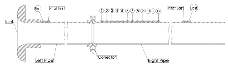
Figure 1: Experimental set up with probe’s positions.

The 5 mm thick polycarbonate wind-pipe has a length of 4400 mm and an inner diameter $D=140.8$ mm. For all the plates (Set 1 and Set 2) the experimental initial conditions are exactly the same, these are summarised in table 1. All plates have the same flow area. The corresponding diameter $d_{i}$ for the classical circular orifice that is used for comparison is 80 mm. The inlet velocity is $U_{0}=5$ m s^-1.

We can define three Reynolds numbers, the bulk Reynolds number based on the inlet condition:

$$Re_{D}={U_{0}D\over\nu}$$ (1)

an orifice Reynolds number based on the orifice diameter and equivalent velocity for the reference circular orifice:

$$Re_{d}={\left(U_{0}{D^{2}\over d^{2}}\right)d\over\nu}$$ (2)

and a local maximum Reynolds number, $Re_{lM}$, based on the maximum velocity $U_{max}$ and the characteristic length over which it is observed. This Reynolds number is measured at the first station $x/D=0.25$ and depends on the plate (see table 2).

Table 1: Experimental conditions for the different sets of plates.

• Experimental conditions
  Inlet velocity, $U_{0}$, m s-1	5
  Reynolds number, $Re_{D}$	39800
  Reynolds number, $Re_{d}$	70000
  Inlet pressure drop, $\Delta p$, kPa	-11.50

There are twelve locations immediately behind the orifice plate (hereafter referred to as “stations”) where the measurements are taken as shown in figure 1. The first station, Station 1, is $0.25~{}D$ behind the plate followed by the remaining eleven stations. The distance between two successive stations is $0.25~{}D$. We conduct hot-wire velocity measurements at these different locations in the pipe and report profiles as functions of the distance from the wall.
A motor driven fan was used to suck down the ambient air into the pipe through the bell mouth and leave through a control valve. The control valve can be regulated to achieve the desired flow velocity in the tunnel. The inlet velocity is checked before each measurement using hotwire anemometry.

For the sake of comparison, it is important to maintain a single uniform inlet velocity condition that will be kept constant for all the measurements. This condition was well satisfied by the bell-mouth inlet. It ensures that the inlet velocity has a flat profile with a single velocity value $U_{0}=5$ m s^-1.

The profile resolution is $\Delta y=5$ mm that is $\Delta y^{*}=\Delta y/D=0.0625$. This was chosen as an optimum between experimental time constraint and profile resolution. It is also consistent with the total width of the hotwire which is of the order of few mm.

3 Fractal orifices

We study two different types of orifice plates, the ‘mono-orifice’ and the ‘complex-orifice’. By ‘mono-orifice’ we mean a single connex hole cut on a plate, by ‘complex-orifice’ we mean a series of disconnected holes cut on a plate.
A mathematical fractal shape is obtained by iterating a pattern at smaller and smaller scales. Strictly speaking the ‘fractal object’ is obtained in the limit of an infinite number of iterations. We adopt this construction approach for our ‘fractal’ orifices and consider different iterations of the pattern corresponding to different achievements of the fractal geometry.
i) The fractal mono-orifices that we use in Set 1 can be thought of as a variation of the classical (smooth) circular orifice which we consider as our reference. We modified the perimeter of the circular orifice to add sharpness and irregularity to this smooth circle. Hence, similarly to the iteration levels of the fractal construction, the edges of the fractal orifice get sharper and sharper at each iteration level.
ii) The fractal complex-orifices in Set 2 make reference to the classical perforated plate with same-sized holes uniformly drilled on the whole surface of the plate. By contrast to the mono-orifice in this case there is no connected flow area.
For each set a total of four fractal orifices $(N=0-3)$ was considered for the present study. All the plates have the same porosity. It is worth noting that when the iteration increases, in order to maintain the porosity the object needs to be scaled down. That is the generator-length in the fractal construction has to be decreased.

3.1 Fractal mono-orifice, Set 1

The fractal orifices that we used for Set 1 (figure 2) are based on the von Koch pattern. This fractal pattern is characterized by a fractal dimension of 1.26. The different iterations of fractal orifices for Set 1 are shown and labelled in figure 2. All the plates have an equal flow area.

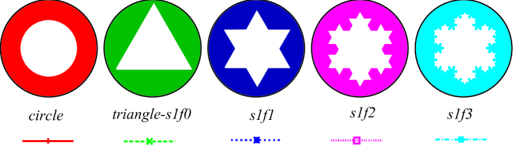
Figure 2: Set 1: classical circular orifice plate, fractal orifice plates with four levels of iteration, s1f0, s1f1, s1f2, s1f3.

The different plates constituting this first set can be classified as orifices, i.e. they can be thought of as a hole with a fractal perimeter. So the natural reference for comparison is the classical circular orifice plate which is the first plate in this set, whereas the second plate s1f0 corresponds to the initial pattern which is just a triangular hole. All the sets except the triangle are symmetric with respect to both the horizontal and vertical planes.

3.2 Fractal complex-orifices, Set 2

Set 2 obeys a different rule, it corresponds to a fractal distribution of holes of different scales. So the natural standard for comparison is a turbulence generated by a series of uniformly distributed identical holes as in the classical perforated plate. The first step which defines the fractal pattern is here just the classical circular orifice. It is labelled circle-s2f0 but is nothing but the previous first plate of Set 1. By contrast to Set 1, Set 2 is more a fractal grid than strictly speaking a fractal orifice. The plates have equal flow area and porosity, the same as in Set 1.

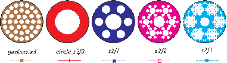
Figure 3: Set 2: classical perforated plate, fractal complex-orifices with four levels of iteration, s2f0, s2f1, s2f2, s2f3.

3.3 Plates classification

From a practical point of view there are two main parameters to consider: the Reynolds number and the porosity. We showed in (Nicolleau et al., 2011) that the shape of the orifice can lead to very different pressure drops and flow patterns and a fractal approach might be a systematic way to classify those shapes . We use the connexity parameter defined in (Nicolleau et al., 2011) indicating when a plate is perforated-like or orifice-like. It is defined as the inverse of the number of holes or closed areas.
Nicolleau et al. (2011) also defined a parameter characterising axi-symmetry, this was measured by the angle of symmetry, that is the smallest angle of rotation leaving the orifice geometry invariant. These non-dimensional parameters are reported table 2.

Table 2: Non-dimensional characteristics for the different plates.

Set	plate porosity symetry connexity scale $Re_{lM}$ $\delta_{g}^{*}$ angle parameter ratio gap
1	circular 0.336 0 1 1 31 000 0.21 triangle 0.336 2.094 ($2\pi/3$) 1 1 29 700 0.05 s1f1 0.336 1.047 ($\pi/3$) 1 0.333 29 100 0.11 s1f2 0.336 1.047 ($\pi/3$) 1 0.111 29 360 0.13 s1f3 0.336 1.047 ($\pi/3$) 1 0.037 27 500 0.14
2	circle 0.336 0 1 1 31 000 0.21 s2f1 0.336 1.047 ($\pi/3$) 0.1429 0.541 14 000 0.06 s2f2 0.336 1.047 ($\pi/3$) 0.0233 0.257 11 500 0.05 s2f3 0.336 1.047 ($\pi/3$) 0.0037 0.111 8 900 0.04 perforated 0.336 0.033 ($2\pi/19$) 0.026 1 7 600 0.04

$Re_{lM}$ is more or less constant for the mono-orifices. This is to be expected as they are basically a variation of the circular orifice: one hole size and one maximum velocity observed around the pipe axis. For the complex-orifices, $Re_{lM}$ varies from large values (as a circular orifice) to small values (as a perforated plate). This is the classical trend for Set 2 which combines features from orifice and perforated plates.

3.4 Velocity profiles

The velocity measurements were conducted for the two sets of orifices using constant temperature hot-wire anemometry which allows a detailed analysis of the effect of the fractal pattern on the flow experiencing the fractal orifice. The hot-wire probe that we used is the 55P16 uni-directional single sensor probe from Dantec Dynamics and the constant temperature anemometer type 54T30. The probe sensing wire is made of platinum-plated tungsten with a diameter of 5 $\mu$m and 1.25 mm long. That is a sensing length to diameter ratio of 250. It can measure velocities from 3 to 50 m s^-1 at a maximum frequency of 10 kHz. The probe was calibrated before each measurement campaign.
We use a single hotwire, the wire is orthogonal to the mean flow direction (pipe axis). Thus we measure a velocity amplitude $U$ that contains the streamwise and the vertical component of the velocity only. The measurements were taken on the centerline and the different statistics are reported as functions of the non-dimensional distance $x/D$ from the plate location. As a reference the velocity was also measured when there was no plate, this corresponds to the data referred to as ‘np’ (i.e. no plate) in the different plots.
The flow in our experiment is not homogeneous, so all the statistics presented are averages in time. We checked over long time samples that our signal is steady. In practice, the time series sampling frequency was $10^{4}$ Hz. Statistics were performed over more than $10^{6}$ points that is for more than 100 s which was large enough to obtain converged statistics. This is more than $10^{4}$ the integral time scales as shown in (Nicolleau et al., 2011). Velocity series are recorded using classical hotwire anemometry. The hotwire is positioned orthogonal to the streamwise direction. So that the recorded velocity takes into account flow fluctuations along two directions and is given by

$$U_{hwa}(t)=\sqrt{U_{x}^{2}(t)+U_{y}^{2}(t)}$$ (3)

where $x$ is the streamwise axis ad $y$ the veraxis. $U_{hwa}$ is recorded as a time series. This velocity as a time series can be decomposed into its mean and fluctuation parts:

$$U_{hwa}=\overline{U}_{hwa}+u$$ (4)

In this paper we present results for the mean value of $U_{hwa}$ that we note just ${U}$:

$${U}=\overline{U}_{hwa}$$ (5)

in section 4. We also present results for the rms of the fluctuation:

$$u^{\prime}=\sqrt{\overline{u^{2}}}$$ (6)

in section 6. In most plots we use no-dimensional quantities: the velocities are normalised by the inlet velocity $U/U_{0}$ and the distances are normalised by the pipe diameter, $x^{*}=x/D$ and $y^{*}=y/D$.

4 Mean velocity profiles

4.1 Velocity profiles for Set 1

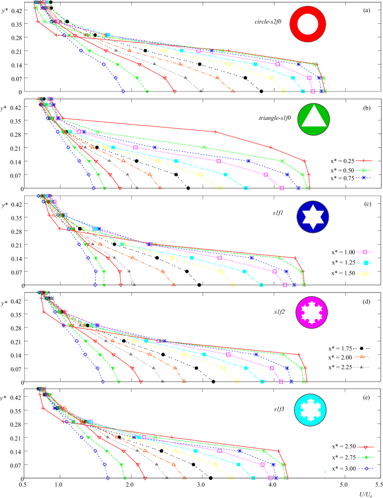
Figure 4: Set 1: Mean velocity profile ${U}/U_{0}$ for different distance $x^{*}$: $+$ 0.25, $\times$ 0.5, $\ast$ 0.75, $\square$ 1, $\blacksquare$ 1.25, $\opencircle$ 1.5, $\fullcircle$ 1.75, $\opentriangle$ 2, $\blacktriangle$ 2.25, $\opentriangledown$ 2.5, $\blacktriangledown$ 2.75 and $\diamond$ 3.

Figure 4, shows the mean velocity profiles, $U$, normalized by the inlet velocity, $U_{0}$ (horizontal axis in the figure), as a function of the distance from the wall $y*=y/D$ (vertical axis in the figure); $y^{*}=0$ at the axis. The vertical increment is 5 mm, that is $\Delta y^{*}=0.07$. The different curves correspond to the different downstream locations $x^{*}$ behind the plates, namely: $+$ 0.25, $\times$ 0.5, $\ast$ 0.75, $\square$ 1, $\blacksquare$ 1.25, $\opencircle$ 1.5, $\fullcircle$ 1.75, $\opentriangle$ 2, $\blacktriangle$ 2.25, $\opentriangledown$ 2.5, $\blacktriangledown$ 2.75 and $\diamond$ 3. Figure 4a, b, c, d and e correspond respectively to the different orifices: circle, triangle, s1f1, s1f2 and s1f3.
The first thing to notice when looking at the different profiles is that the triangular orifice plate s1f0 has to be set apart. The profiles’ evolution for all the other plates is similar. For these plates, at $x^{*}=0.25$, the magnitude of the velocity near the wall is smaller than at other stations. This is because near the wall and near the plate a re-circulation zone exists. This re-circulation zone vanishes further away from the plate.

In the case of s1f0-triangle, the vertex of the triangular flow area disrupts the re-circulation zone near the wall, we will see more evidence of this latter on. The asymmetrical flow area of s1f0 could also be the reason behind its atypical behaviour.

All the plots are on the same scale, so another noticeable feature is that the velocity decreases from (a) to (e). Hence the higher the fractal iteration level the smoother the perturbation to the flow. This trend however is not true for all distances from the plate and we will discuss this in more details with figure 6.

From figure 4 we can also see that the first two profiles $x^{*}=0.25$ and $x^{*}=0.5$ behind the circular orifice plate, collapse on each other for $y^{*}>0.25$. This is the well-known “vena contracta” effect for circular orifices. This effect is also present in the other orifices, except again for the triangular-shaped orifice. The vena contracta effect is more pronounced in the case of the circular orifice with close profiles up to $x^{*}=0.75$, whereas for the fractal orifices it disapears after $x^{*}=0.5$. One possible explanation is that the circular orifice can be described as monoscale, meaning that it can be defined by one scale only, its diameter; whereas the other plates can be described as multiscale in that they are forcing on a range of scales. The fractal distribution of sharp edges is thought to enhance mixing as observed in the numerical experiment of van Melick and Geurts (2012).

4.2 Measure of self-similarity in profiles for Set 1

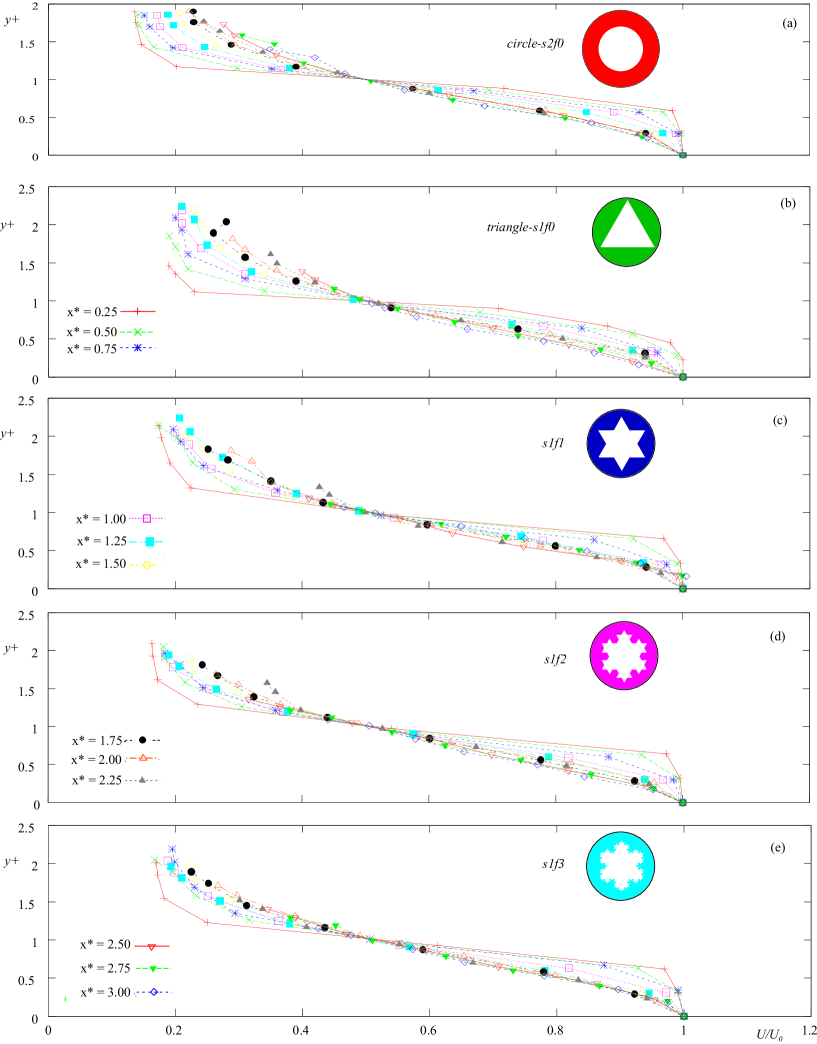
Figure 5: Set 1: normalized velocity profiles (${U^{*}}$, $y*$), for different distance $x^{*}$: $+$ 0.25, $\times$ 0.5, $\ast$ 0.75, $\square$ 1, $\blacksquare$ 1.25, $\opencircle$ 1.5, $\fullcircle$ 1.75, $\opentriangle$ 2, $\blacktriangle$ 2.25, $\opentriangledown$ 2.5, $\blacktriangledown$ 2.75 and $\diamond$ 3.

In figure 5 we use the classical velocity normalisation to look for some trends of self-similarity in the mean velocity profile, on the horizontal axis we report the velocity divided by the axial mean velocity (which is also the maximum velocity):

$$U^{*}={{U}(y)\over{U}(0)}$$ (7)

on the vertical axis we report the distance to the wall normalised by the distance at which the velocity is half that at the centerline

$$y^{+}={y\over y_{1\over 2}}$$ (8)

where ${U}(y_{1\over 2})={U}(0)/2$ by definition. So that all normalised profiles go through the fixed point $(U^{*}=1/2,y^{+}=1)$. The spreading of the profile around that fixed point is an indication of how self-similar they are.
The notations and symbols are the same as in figure 4. The different curves correspond to the different downstream locations behind the plates $x^{*}$, namely: $+$ 0.25, $\times$ 0.5, $\ast$ 0.75, $\square$ 1, $\blacksquare$ 1.25, $\opencircle$ 1.5, $\fullcircle$ 1.75, $\opentriangle$ 2, $\blacktriangle$ 2.25, $\opentriangledown$ 2.5, $\blacktriangledown$ 2.75 and $\diamond$ 3. Figure 4a, b, c, d and e correspond respectively to circle, triangle, s1f1, s1f2 and s1f3.
The values of $y^{+}$ are smaller than 2 for the circular orifice, whereas there are values above 2 for the other orifices, so near the wall, the profiles are less spread for the circular orifice than for the other orifices. However, far from the wall, the circle and triangle plates show the most spread profiles, whereas for the fractal orifices s1f1, s1f2 and s1f3 the profiles tend to a universal shape which is very close to

$$U^{*}\simeq 2y^{+}$$ (9)

for $0.3<y^{+}<0.9$. For the three highest fractal iterations a universal profile is nearly achieved after one diameter. The higher the iteration the better the collapse of the profile for $x^{*}>1$. The upper parts of the profiles ($y^{+}>1$) show more spread. This corresponds to data measured close to the wall which are less accurate owing to the wall boundary condition: $U\to 0$ when $y^{*}\to 0.5$, whereas our hotwire limitation is around 3 m s^-1.

4.3 Fractal scaling effects at each station

It is not easy to see directly the fractal scaling effects on the profile from the previous figures.

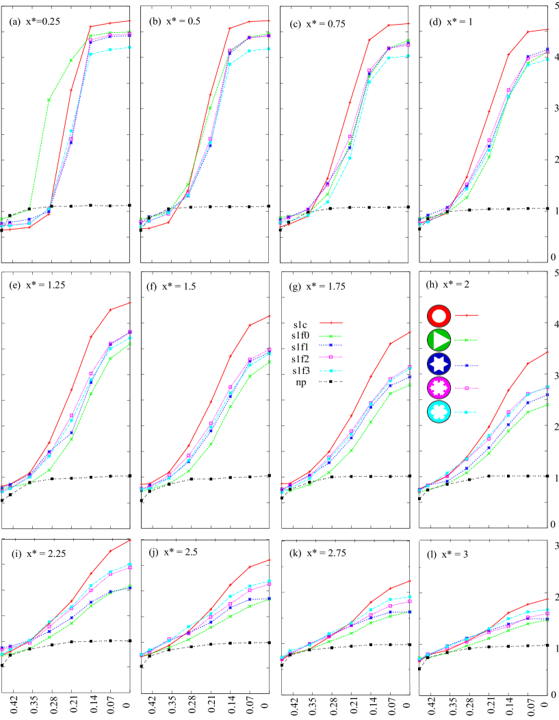
Figure 6: Set 1: Comparison of fractal iteration level effects on velocity profiles ($y^{*}$, ${U}/U_{0}$) for the different stations.

To make it clearer in figure 6 we compare the different iteration levels at a given station. The velocity is normalized by the inlet velocity (${U}/U_{0}$ on the vertical axis) and is plotted as a function of $y^{*}$. Figure 6 presents the same profiles as in figure 4 but this time grouped by stations so that we can discuss directly the effect of the fractal iteration level on the profiles. For the sake of comparison the profile measured without any plate has also been included. The different figures (a-l), correspond respectively to $x^{*}=0.25$, 0.5, 0.75, 1, 1.25, 1.5, 1.75, 2, 2.25. 2,5. 2.75 and 3. The color coding and line symbol correspond to that in figure 2.
The figure shows that far from the orifice, $x^{*}=3$, the circular orifice shows the lowest decrease in velocity and the triangle orifice the largest decrease. The triangular orifice decays more slowly initially and then has a more rapid decay further downstream. The fractal-orifices show intermediary behaviour:

• $x^{*}\leq 1$ close to the orifice, the higher the fractal iteration the lower the velocity level,

• $x^{*}\geq 2$ far from the orifice, the higher the fractal iteration the higher the velocity level.

Further down than $x^{*}=2.25$ there is little difference between the fractal orifices for $y^{*}>0.14$.

4.4 Set 2: Mean velocity profiles

Figure 7 shows the mean velocity profile for Set 2, ${U}$, normalized by the inlet velocity, $U_{0}$, as a function of the distance from the pipe axis $y^{*}$ and for the different downstream locations $x^{*}$.

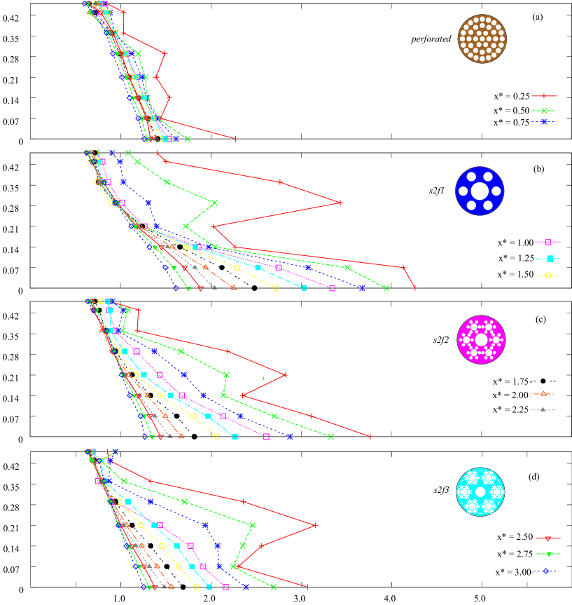
Figure 7: Set 2: Velocity profiles ${U}/U_{0}$ (horizontal axis) as functions of $y^{*}$ (vertical axis).

The top panel is the reference classical perforated plate that is often used as a flow conditioner. The different plots correspond respectively to (a) the classical perforated plate, (b) s2f1, (c) s2f2 and (d) s2f3. We omitted the circular orifice in this figure the results for that plate have already been shown with the results for Set 1 (figure 4).
Near the plate, the profiles for the fractal complex-orifices show more than one peak as for the perforated plate. This illustrates the fundamental difference between Set 2 and Set 1. In Set 1 the flow is acted upon from the orifice’s perimeter, whereas Set 2 corresponds to jets fractally distributed in space and scale interacting with each other. The peaks are smoothed out after $x^{*}=1$ for all the plates, with no intermediary velocity peak between the wall and the pipe centre.
In figure 8 we compare the effect of each complex-orifice at a given station. The first observation is that the mean velocity near the pipe axis decreases as the fractal iteration level increases. This can be observed consistently at each station.

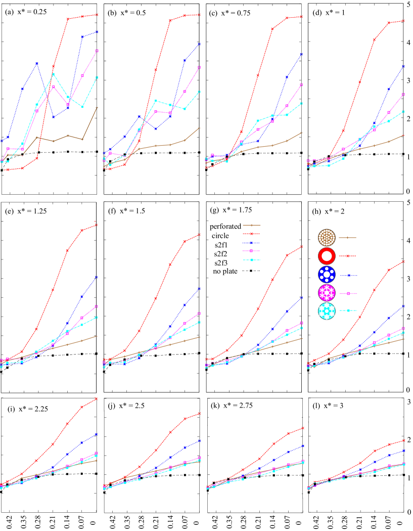
Figure 8: Set 2: Comparison of scaling effects on velocity profile normalized by inlet velocity, $U_{0}$, at each station.

The three fractal complex orifices s2f1, s2f2 and s2f3 loose their two-peak profile shape at about the same station $x^{*}=0.75$. s2f2 and s2f3 have very close profiles at all stations with peaks at the same $y^{*}$.

The return to a low smooth profile is faster across the classical perforated plate until $x^{*}=2$. Then as the fractal iteration level increases, the velocity profiles get closer to that of the reference perforated plate. However, the velocity profiles of the lower fractal iteration level s2f1 depart significantly from those of s2f2, s2f3 and the classical perforated plate, even as far downstream as $x^{*}=3$. s2f1 keeps a behaviour intermediary between the orifice and the perforated plate. There is little difference between the profiles of s2f2 and s2f3 after $x^{*}=1.75$ indicating that there is little to gain in manufacturing plates for higher fractal order than 2. This is consistent with findings in (Nicolleau et al., 2011). Of course this conclusion is only valid for the Reynolds number we have here. As the Reynolds number increases one can expect more discrepancies between s2f2 and s2f3.
To summarise, the fractal complex-orifices s2f2 and s2f3 generate high velocity values near the plate, values that are close to the circular orifice values; but further downstream, $x^{*}>2$, the velocity decreases rapidly down to the level of the perforated plate. There is a clear effect of the fractal iteration as this is not true for s2f1.

5 Guessed volume flow rates

As the density is constant in our experiment the mass conservation reduces to the volume flow rate conservation. That is

$${\cal V}(x)=\int_{0}^{1}\int_{0}^{2\pi}\overline{U}(x,y,\phi)\,ydyd\phi$$ (10)

is independent of $x$. Furthermore, when the flow is axi-symetric the volume flow rate ${\cal V}$ (10) reduces to:

$${\cal V}(x)=2\pi\int_{0}^{1}y\,\,\overline{U}(x,y)dy$$ (11)

and is known from the velocity profile. From the profiles we measured, we can use (11) as a measure of axi-symmetry. Indeed if the flow were axi-symmetric (11) would give the same value at all stations. An equivalent flow rate can be computed from the profiles obtained after the fractal orifice as if the flows were axi-symmetric. In practice, such an equivalent flow rate will converge towards the actual volume flow rate as we get further away from the plate and the flow reverts to an axi-symmetric shape. There is another factor to take into account which is that the velocity we measure is $\overline{U}_{hwa}(y)$ not $\overline{U}(y)$. So, large velocity fluctuations along the $y$ axis and recirculation effects near the wall will also affect our estimation of the flow rate. However, $\overline{U}_{hwa}(y)\not\simeq\overline{U}(y)$ is also an effect of the fractal shapes and calculating the volume flow rate from the profiles given in figure 5 and figure 7 will still reveal the influence of the fractal orifices on the flow and how they force or delay the return to axi-symmetric profiles.
In figure 9 we plot ${\cal V}(x^{*})/{\cal V}_{0}$, the guessed flow rate normalised by the inlet flow rate. (a) corresponds to the mono-orifice type plates from from Set 1 and (b) to the complex-orifice type plates from Set 2.

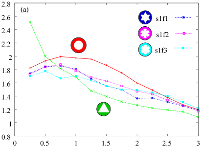
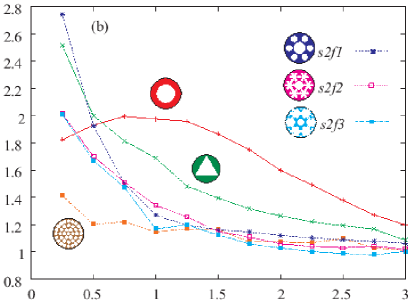
Figure 9: Evolution of ${\cal V}/{\cal V}_{0}$ as a function of $x^{*}$ for the two types of plates: (a) Set 1, (b) Set 2.

As noticed before, the triangle orifice behaviour in figure 9a is at odds with the other orifice plates. It is clear from figure 9a that its behaviour is closer to the behaviour for complex orifices though it is obviously a mono-orifice. Omitting the triangle plate one can conclude that the guessed flow rate for the mono-orifices reflect the ‘vena contracta’ effect. The streamlines are deflected by the orifice resulting in increased velocities near the axis and the development of a re-circulation zone (with negative velocities) near the wall. The hotwire only measures the velocity modulus down to $U\simeq 3$ m s^-1. So our guessed volume flow rate is clearly an overestimation in the vena contacta region. From figure 9 we can estimate the position of the vena contracta and of the maximum thickness of the recirculation zone. This is around $x^{*}=1$ for the circular orifice and is closer to the plate for the fractal orifice around $x^{*}=0.75$ for s1f2 and s1f3 and probably closer for s1f3 but we do not have the necessary precision to conclude for that orifice plate. (The vena contracta effect also explains the difficulty encountered in (Nicolleau et al., 2011) when trying to apply directly Mazellier and Vassilicos (2010)’s evolution law for the maximum of $u^{\prime}$.)
Further down all the profiles converge to the same asymptotic curve after $x^{*}=2.25$. But the trend is still to a decrease and we can conclude that the flow has not yet fully reverted to axi-symmetry at $x^{*}=3$. All the fractal orifices profiles for s1f1, s1f2 and s1f3 are similar. So that we can conclude that in terms of return to axi-symmetry the first fractal level s1f1 is already optimum.
Figure 9b shows the evolution of the guessed flow rate for the perforated type plates from Set 2. They all show the same trend near the plate that is an over-prediction of the flow rate and a monotonic decrease as $x^{*}$ increases. This is also the trend followed by the triangular-shaped orifice. This is actually due to the interaction of the flow coming from the plate and the boundary layer near the wall. Indeed the common feature between all these plates including the triangle orifice is the smallest distance from the wall to the flow area. To characterise this effect we define a new non dimensional number $\delta_{g}^{*}$ as

$$\delta_{g}^{*}=\delta_{g}/D$$ (12)

where $\delta_{g}$ is the smallest distance from the flow area to the wall. Values of $\delta_{g}^{*}$ are reported in table 2. The complex-orifices and triangular shaped orifice have all $\delta_{g}^{*}<0.06$, whereas the other orifice-like plates have all $\delta_{g}^{*}>0.11$.

6 Velocity fluctuation RMS profiles

6.1 Set 1: RMS profiles

The rms profiles behind the plates in Set 1 are shown in figure 10.

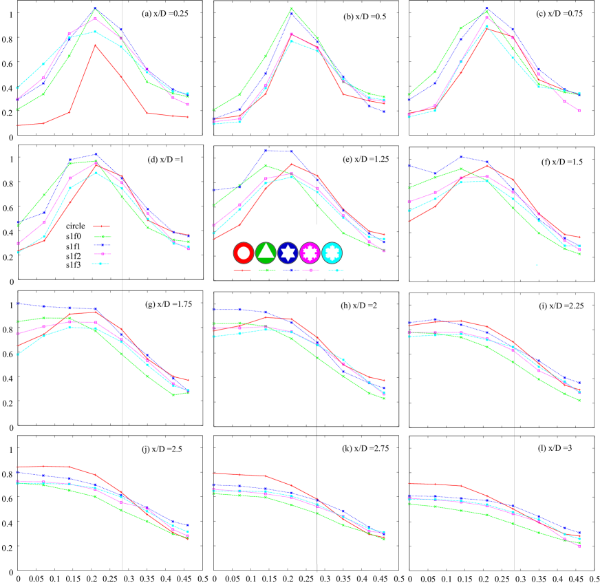
Figure 10: Set 1: $u^{\prime}/U_{0}$ (vertical axis) as functions of $y^{*}$ (horizontal axis) at different station $x^{*}$. The vertical lines crossing the plots indicate the position of the circular orifice’s edge.

The position of the circular orifice’s edge is indicated by a light vertical line. The fractal perimeters have no much effect on the rms outside the area of the circular orifice except for the triangular orifice which apex is clearly outside the area delimitated by the circular orifice (for Set 1 $\delta_{g}^{*}$ varies from 0.05 for the triangular orifice to 0.21 for the circular orifice) and has an influence on the boundary layer developing from the pipe’s wall.
Most of the effect of the fractal edges is therefore concentrated within the area delimitated by the circular shape. Within that area, there is little effect of the fractal perimeter on the position of the maximum for $u^{\prime}$. Near the plate ($x^{*}=0.25$) the peak of $u^{\prime}$ is observed at the same position for all plates, that is around $y^{*}=0.2\pm 0.05$. For the circular orifice, for as long as there is a peak for $u^{\prime}$ it stays at $y^{*}=0.2$.
Close to the plate up to $x^{*}\simeq 1D$, the fractal orifices give higher turbulence fluctuations than the classical circular orifice and the higher the fractal iteration the lower $u^{\prime}$. For $x^{*}>1D$ the triangle’s profile departs from the general trend followed by the fractal perimeter, its overall profile is now significantly influenced by the portion outside the area delimitated by the circular shape. For the other plates s1f1, s1f2, s1f3, the higher the fractal iteration the lower $u^{\prime}$. This is observed at any distance from the orifice.
Further than $x^{*}=2.25$ from the plate, the fractal orifices yield lower turbulence fluctuations than the circular orifice within the circular delimitated area. They also generate flatter profiles indicating a faster flow recovery. As expected the further from the plate the less differences between the different fractal orifices. There is little differences between s1f2, s1f3 as close to the plate as $x^{*}=2$.

6.2 RMS profiles Set 2

Figure 11 shows the rms profiles behind the different complex-orifices from Set 2. For the sake of comparison the profiles from the classical perforated plate are added to the plots and the position of the circular orifice’s edge is indicated by a light vertical line.

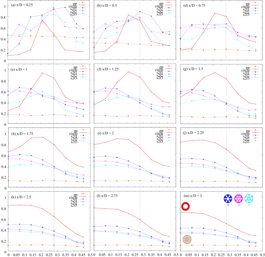
Figure 11: Set 2: $u^{\prime}/U_{0}$ (vertical axis) as functions of $y^{*}$ (horizontal axis) at different stations $x^{*}$

The effect of the complex-orifices is clear from the onset: just after the orifice, there is not a single-peaked profile as for the circular orifice but the profiles for the complex-orifices are higher and flatter. They are also higher than that of the perforated plate except at the pipe centre for the lower order fractal orifices.
Far from the plate position, the profiles seem to converge towards the flat level profile obtained with the perforated plate. There is a clear effect of the fractal iteration level on that convergence: the higher the level, the closer to the perforated plate results. After $x^{*}=2.25$ there are little differences between s2f2 and s2f3.
Similarly to Set 1, the fractal orifices first give turbulence levels higher than those of the circular orifice. Then the complex-orifices’ turbulence fluctuation decreases rapidly while that of the circular orifice increases before reaching a smoother-shaped profile. As can be seen in figure 11a, by contrast to Set 1 the complex orifices are acting outside the area delimitated by the reference circular orifice. So eventually their profile get lower than that of the circular orifice even outside the delimitated area. After $x^{*}=1.75$ the complex-orifices’ profiles are always smaller than the circular orifice’s profile and much closer to the perforated plate profile.
To quantify the production of turbulence energy $u^{\prime 2}$ relative to each orifice we can define the non-dimensional parameter $\alpha$ as follows:

$$\alpha_{i}(x^{*})=\max_{y^{*}}{u^{\prime}_{i}(x^{*})\over u^{\prime}_{p}(x^{*})}$$ (13)

where $i$ designates a particular orifice and $p$ stands for the classical perforated orifice that we take as our reference. $\alpha$ is defined for each orifice as a function of $x^{*}$. It measures the production of velocity fluctuation relative to the classical perforated orifice. The values of $\alpha$ are reported in figure 12 for Set 1 and Set 2.

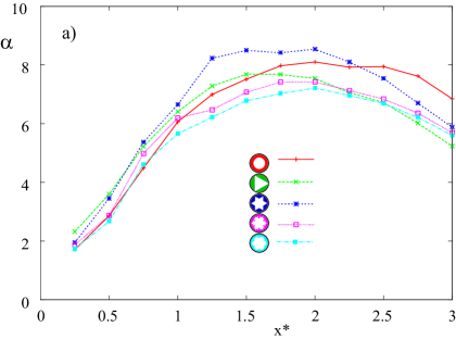
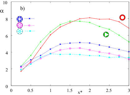
Figure 12: $\alpha$ as a function of $x^{*}$ for the different orifices in a) Set 1, b) Set 2

All the orifices show the same trend for $\alpha$, it first increases and then decreases showing a maximun in the range $1\leq x^{*}\leq 2$. There is a clear fractal iteration effect: the higher the iteration the lower $\alpha$. s2f3 as the highest iteration looks as an interesting limiting case: the decrease of $\alpha$ with $x^{*}$ is very small and it seems that the flow after s2f3 will retain a much higher turbulence level than the reference perforated plate for a very long distance.
The different iterations in both sets correspond to different scale ratios (see table 2). Furthermore, in Set 2, different connexity parameters are linked to different scale ratios. These two quantities basically tell us the range of scales forced at the orifice (scale ratio) and how many of them there are (how many holes is the connexity parameter). So decreasing the connexity, (and scale ratio) is like forcing on a larger range of scales and a less confined physical space and indeed that flattens the rms profiles and decreases the maximum values reflected by $\alpha$.

7 Conclusion

It was shown in (Abou-El-Azm et al., 2010; Nicolleau et al., 2011) that fractal orifices yield lower pressure drops than the popular circular orifice; a very important property for flowmetering applications. That initial study needed to be completed by an assessment of how disruptive to the flow the fractal-orifices are when compared to the two benchmarks that are the circular orifice and perforated plate. (This latter was chosen for its standard flow mixing properties as it is not relevant of course for flowmetering.) In particular, a question one may ask is: how long it takes for the fractal-generated flow to return to axi-symmetry and smooth out the high turbulence levels it may generate?

This paper compares the merits of different orifice plates for the two reference classes: mono-orifice and complex-orifice, for a rapid return to axi-symmetric flow. The guessed flow rate is introduced as an objective measure of how disruptive is the orifice to the flow in view of flowmetering techniques.

The results show that for the mono-orifice an important feature to consider is the interaction of the object with the re-circulation zone from the wall. The parameter $\delta_{g}^{*}$ is introduced to measure the smallest gap between the flow area and the wall. For the mono-orifice with $\delta_{g}^{*}>0.05$ the return to axi-symmetry is better than that of the circular orifice but there is no significant effect of the fractal iteration. (At least for the Reynolds number used here.)

For the complex-orifice the return to axi-symmetry is always better than that of the circular orifice. There is a clear effect of the fractal iteration near the plate, though as for the mono-orifice, for that Reynolds number there is an optimum iteration ($s2f2$) above which there is no significant effect of the iteration.

In terms of turbulence intensity as measured by the factor $\alpha$ the fractal-orifices are always better than the circular orifice after $\sim 2.5$ diameter. The complex-orifices seem particularly good for that purpose.
Overall, the results confirm the potential of fractal orifices as flowmeters. It was previously known that they are more efficient in terms of pressure drop. The present study indicates that they are also more efficient in re-generating an axi-symmetric flow with lower level of velocity fluctuations. This is also very important for applications to flowmetering where a standard flow after the orifice is required for robust accurate measurements.
For the Reynolds number used here, there is an optimum iteration of the fractal level above which no improvement to the flowmeter is to be expected. So we expect in future works to be able to define the range of useful iterations for a given range of Reynolds numbers. The main parameters proposed for the characterisation of the fractal orifice are the connexity parameter, the symmetry angle and gap to the wall $\delta^{*}_{g}$. But more work with more geometries needs to be done to investigate all these parameters.
There is also a need for validation of more complex subgrid models dealing in particular with rough surfaces (Laizet and Vassilicos, 2009; Anderson and Meneveau, 2011; Lopez Penha et al., 2011; van Melick and Geurts, 2012) and fractal-forced flows could provide a systematic way to generate data for such validations. In particular it is easy to see that such flows pose a real challenge to grid-dependent method as Detached Eddy Simulation (Zheng et al., 2010).

References

References

- Abou-El-Azm et al. (2010) Abou-El-Azm A, Chong C, Nicolleau F and Beck S 2010 Experimental Thermal and Fluid Sc. 34, 104–111. doi:10.1016/j.expthermflusci.2009.09.008.
- Anderson and Meneveau (2011) Anderson W and Meneveau C 2011 J. Fluid Mech. 679, 288–314. doi:10.1017/jfm.2011.137.
- Farge et al. (1993) Farge M, Hunt J and Vassilicos J 1993 Wavelets, fractals and Fourier transforms Clarendon Press, Oxford.
- Laizet and Vassilicos (2009) Laizet S and Vassilicos J C 2009 Journal of Multiscale Modelling 1(1), 177–196.
- Lopez Penha et al. (2011) Lopez Penha D J, Geurts B J, Stolz S and Nordlund M 2011 Computers and Fluids 51, 157-173.
- Manshoor et al. (2011) Manshoor B, Nicolleau F and Beck S 2011 Flow Measurement and Instrumentation 22(3), 208–214. doi: 10.1016/j.flowmeasinst.2011.02.003.
- Mazellier and Vassilicos (2010) Mazellier N and Vassilicos JC 2010 Phys. Fluids 22(7), 07510. doi:10.1063/1.3453708.
- van Melick and Geurts (2012) van Melick P.A.J and Geurts B.J. 2012 Fluid Dyn. Res.
- Meneveau (1991) Meneveau C 1991 J. Fluid Mech. 224, 429–484.
- Meneveau and Sreenivasan (1990) Meneveau C and Sreenivasan K R 1990 Physical Review A 41(4), 2246–2248.
- Michelitsch et al. (2009) Michelitsch T, Maugin G, Nicolleau F, Nowakowski A and Derogar S 2009 Phys. Rev. E 80, 011135. doi:10.1103/PhysRevE.80.011135.
- Nastase et al. (2011) Nastase I, Meslem A and Hassan M E 2011 Fluid Dyn. Res. 43, 065502. doi:10.1088/0169-5983/43/6/065502.
- Nicolleau (1996) Nicolleau F 1996 Phys. Fluids 8(10), 2661–2670.
- Nicolleau et al. (2011) Nicolleau F, Salim S and Nowakowski A 2011 Journal of Turbulence 12(44), 1–20. doi: 10.1080/14685248.2011.637046.
- Nicolleau and Vassilicos (1999) Nicolleau F and Vassilicos J 1999 Phil. Trans. R. Soc. Lond. A 357(1760), 2439–2457. doi: 10.1098/rsta.1999.0441.
- Nowakowski et al. (2011) Nowakowski A, Nicolleau F and Salim S 2011 in ‘6th AIAA Theoretical Fluid Mechanics Conference’ Hawaii Convention Center Honolulu, Hawaii, USA p. (ID: 1023232).
- Seoud and Vassilicos (2007) Seoud R E and Vassilicos J C 2007 Phys. Fluids 19(10), 105108.
- Sreenivasan et al. (1989) Sreenivasan K R, Ramshankar R and Meneveau C 1989 Proc. R. Soc. Lond. A 421, 79–108.
- Valente and Vassilicos (2012) Valente P C and Vassilicos J C 2012 Phys. Lett. A 376, 510–514.
- Zheng et al. (2010) Zheng H, Nicolleau F and Qin N 2010 in S Peng, P Doerffer and W Haase, eds, ‘Notes on Numerical Fluid Mechanics: 3rd Symposium on Hybrid RANS-LES Methods’ Vol. 111 Gdansk, Poland Gdansk, Poland pp. 157–165. doi: 10.1007/978-3-642-14168-3-13.