Generating Log-normal Mock Catalog of Galaxies in Redshift Space

Abstract

We present a public code to generate a mock galaxy catalog in redshift space assuming a log-normal probability density function (PDF) of galaxy and matter density fields. We draw galaxies by Poisson-sampling the log-normal field, and calculate the velocity field from the linearised continuity equation of matter fields, assuming zero vorticity. This procedure yields a PDF of the pairwise velocity fields that is qualitatively similar to that of N-body simulations. We check fidelity of the catalog, showing that the measured two-point correlation function and power spectrum in real space agree with the input precisely. We find that a linear bias relation in the power spectrum does not guarantee a linear bias relation in the density contrasts, leading to a cross-correlation coefficient of matter and galaxies deviating from unity on small scales. We also find that linearising the Jacobian of the real-to-redshift space mapping provides a poor model for the two-point statistics in redshift space. That is, non-linear redshift-space distortion is dominated by non-linearity in the Jacobian. The power spectrum in redshift space shows a damping on small scales that is qualitatively similar to that of the well-known Fingers-of-God (FoG) effect due to random velocities, except that the log-normal mock does not include random velocities. This damping is a consequence of non-linearity in the Jacobian, and thus attributing the damping of the power spectrum solely to FoG, as commonly done in the literature, is misleading.

1 Introduction

Galaxy redshift surveys, mapping the three-dimensional distribution of galaxies, have been one of the most powerful tools in modern cosmology (see, for example, [1]). Specifically, measurements of the galaxy two-point correlation function or its Fourier counterpart, power spectrum, allow us to extract cosmological information via, e.g., baryon acoustic oscillations and the redshift-space distortion (BAO and RSD, see e.g. [2] for recent measurements). Galaxy surveys complement other cosmological probes such as temperature anisotropies and polarization of the Cosmic Microwave Background (CMB; [3, 4]) and luminosity distances of Type Ia supernovae [5, 6].

Deducing robust cosmological constraints from galaxy surveys requires an accurate modelling of the observed two-point correlation function and power spectrum along with their covariance matrices. This is a challenging task because of non-linearity and non-Gaussianity of the galaxy density field. First, non-linear gravitational evolution transforms a nearly Gaussian initial density field into a non-Gaussian one [7], and the galaxy density field is related non-linearly to this non-Gaussian matter density field (galaxy bias; see [8] for a review). In addition, the observed galaxy density field differs from the underlying one because of systematics due to peculiar velocity (RSD) and variations in observing conditions across the survey area (window function effect).

Due to these various non-linearities, unlike for the CMB analysis, the Gaussian approximation is no longer valid for computing the covariance matrix of the galaxy two-point statistics. Going beyond the Gaussian approximation, a method based on non-linear perturbation theory including contributions from connected four-point functions can model the non-linear covariance matrix on quasi-linear scales [9, 10]. Perturbative approaches break down on small scales where non-linearities are too strong. The gravitational amplification and galaxy bias in these non-linear scales may be fitted by a number of free parameters of effective field theory [11, 12]. However, treatment of the mode-coupling effect due to the survey window function (for example, due to sparse sampling of the survey area [13]) requires a full account of modes down to the resolution scale of the survey, set by the number density of the sample: $\bar{n}_{g}\gtrsim 1/P(k)$, $P(k)\equiv\left|\delta(\mbox{\boldmath$k$})\right|^{2}$ being the power spectrum of the overdensity field $\delta(\mbox{\boldmath$x$})$.

Cosmological N-body simulations have been the gold standard in modelling non-linearity in the large-scale structure. As phenomena in a wide range of scales are involved in the formation and evolution of galaxies, simulating all the relevant physics of the formation and evolution of galaxies is impractical. Instead, the usual practice is to “paint” galaxies onto the halos in matter-only simulations by using the halo-occupation distribution (HOD) function estimated from, for example, the angular clustering of the survey (e.g., [14]), or by using Subhalo Abundance Matching (SHAM) with the observed stellar mass function (e.g., [15]. With these mock galaxy samples from the simulation at hand, the galaxy correlation functions and their covariance matrices can be measured directly from a suite of N-body simulations including various selection effects of the surveys. Even for these matter-only N-body simulations, however, a robust cosmological parameter estimation may demand too large computational resources. This is because estimating the covariance matrix from N-body simulations hampers the cosmological parameter estimation by a factor of $1+N_{b}/N_{s}$, where $N_{s}$ is the number of N-body simulations and $N_{b}$ is the number of independent bins used for the estimation of parameters [16]. If we were to achieve a percent precision on the covariance matrix, we would need $N_{b}/N_{s}=10^{-2}$. As $N_{b}\approx 10^{2}$ for typical survey data, $N_{s}\approx 10^{4}$ would be required. This requirement would become more severe in estimating the inverse covariance matrix and its associated errors (see e.g., [17, 1, 18]).

One pragmatic way of bypassing this problem is to simulate gravitational evolution by adopting a set of simplified assumptions. In this approach, one trades accuracy for speed of simulations, especially on small scales. For example, the Zel’dovich simulation [19] captures correct density and velocity fields on large scales where non-linearities are modest; the higher order Lagrangian perturbation theory (LPT [20, 21, 22]) simulations capture non-linearities on progressively smaller scales [23, 24, 25, 26, 27, 28]. We refer the readers to Ref. [29] for a recent review and to Refs. [30, 31, 32] for comparisons between different approaches.

In this paper, we shall take a different approach: instead of modelling the non-linear density evolution, we exploit statistical properties of the non-linear galaxy density field. Specifically, we generate a mock galaxy catalog with the assumption that the probability density function (PDF) of galaxy density fields follows a log-normal distribution. This assumption is based upon the observation that the PDF of log-transformed density fields, $\ln(1+\delta)$ with $\delta\equiv n/\bar{n}-1$ being the density contrast, measured from N-body simulations roughly matches a Gaussian PDF [33, 34, 35, 36, 37, 38]. The evidence for a log-normal PDF does not only come from the matter density fields in simulations, but also from the Dark Energy Survey (DES) science verification data [39] and earlier measurements [40, 41].

Note that log-normality is not merely a statement about the one-point PDF, but it means that the log-transformed field $\ln(1+\delta)$ is a multi-variate Gaussian random field whose statistics are completely specified by its two-point correlation function. For this, the N-body simulation of Ref. [42] has confirmed that the two-point correlation function of matter density fields also roughly matches the prediction of log-normality well into fairly non-linear regime.

In addition, the log-normal mock generator presents the following practical advantages that further motivate our pursuing this approach:

1. It is fast. Since the relation between the density fields and the Gaussian (log-transformed) fields is given by a local transformation (see section 3 for more details), the log-normal mock generator is almost as fast as generating three-dimensional Gaussian random fields. This allows us to quickly generate a large number of mock galaxy distributions.

2. It is direct. The log-normal mock generator takes the observed galaxy two-point correlation function as an input so that we can avoid post-processing steps (halo finding, HOD, for example) connecting the non-linear density field to mock galaxies.

3. It is instructive. Upon assuming log-normal PDF of the galaxy density field, all higher-order correlation functions are given in terms of the two-point correlation function of the log-transformed field [33]. This allows us to quantitatively study highly non-linear mode-coupling effects in both the signal and covariance matrix that demand knowledge about the density field on non-linear scales. One such example is mode-coupling due to the survey window function. By using a thousand log-normal mock catalogs, Ref. [13] has quantified the effect from a duplicated, sparse (instead of contiguous) angular selection function, and deduced the optimal analysis strategy.

In this paper, we extend the real-space log-normal mock generator presented in Ref. [13] by including the velocity field in a consistent manner. We then generate the log-normal mock in redshift space by applying the real-to-redshift space mapping. Again, equipped with perfect knowledge about the statistical properties of the galaxy density and velocity fields, such a mock catalog serves as an excellent test bed for modelling RSD due to this non-linear mapping [43]. To test the RSD effect on the two-point statistics of the log-normal mock catalog, we begin with the real-space galaxy two-point correlation function as an input. We use a log-normal PDF to generate a three-dimensional galaxy density field, as well as a matter density field. Finally, we generate a velocity field consistent with the matter density field by using the linearised continuity equation (see section 3 for more details). We then measure the galaxy two-point statistics (correlation function and power spectrum) both in real and redshift space, and the pairwise line-of-sight velocity PDFs from the log-normal mock catalog. We also calculate the mean pairwise velocity using log-normal statistics and show that it agrees with the measurement from the catalog.

Our implementation of log-normal galaxy density and velocity fields differs from other log-normal codes such as [44], FLASK [45] and CoLoRe [46]. FLASK does not have a prescription for producing a velocity field; hence one has to provide an anisotropic power spectrum when generating density fields in redshift space. CoLoRe generates a velocity field by using linear theory velocities corresponding to the log-transformed field, so the resulting velocities follow a Gaussian PDF. Note that the fact that the velocity field follows a Gaussian PDF does not imply that the pairwise line-of-sight velocity PDF is Gaussian because the pairwise line-of-sight velocity PDF is a pair-weighted quantity (see section 2 for more details). In contrast, in this paper, we use the linearised continuity equation to ensure mass conservation with little additional computing cost compared to the CoLoRe method.

The rest of the paper is organized as follows. In section 2 we present an overview of redshift-space statistics including the two-point correlation function and the pairwise line-of-sight velocity PDF. In section 3 we introduce our method to generate log-normal density and velocity fields. In section 4 we present measurements from our log-normal mock catalogs, including two-point statistics in real space (sec. 4.1.1), the cross-correlation coefficient between matter and galaxy fields (sec. 4.1.2), two-point statistics in redshift space (sec. 4.2), and pairwise line-of-sight velocity PDFs (sec. 4.3); in sec. 4.4 we discuss how the streaming model reduces to the Kaiser limit at large separations. We summarize the results in section 5. In appendix A, we present a derivation of the streaming model for RSD. In appendix B, we lay out the method that we use to correct for the binning effect when measuring power spectra. In appendix C, we present the details of calculating the mean pairwise line-of-sight velocity from the log-normal mock catalogs. The code documentation of our log-normal mock generator is in appendix D. Throughout, we use the following Fourier convention:

$$f(\mbox{\boldmath$k$})=\int d^{3}xf(\mbox{\boldmath$x$})e^{-i\mbox{\boldmath$k$}\cdot\mbox{\boldmath$x$}},~{}f(\mbox{\boldmath$x$})=\int\frac{d^{3}k}{(2\pi)^{3}}f(\mbox{\boldmath$k$})e^{i\mbox{\boldmath$k$}\cdot\mbox{\boldmath$x$}}\,.$$ (1.1)

In this paper, the term real space refers to the contrast with redshift space, and the term configuration space refers to the contrast with Fourier space.

2 Review of RSD

In spectroscopic galaxy redshift surveys, radial distances to galaxies are inferred from observed spectral shifts containing both the Hubble expansion and peculiar velocities of galaxies along the line-of-sight. The observed positions (redshift space) of galaxies are related to the true positions (real space) of galaxies by

$$\mbox{\boldmath$s$}=\mbox{\boldmath$x$}+\frac{1}{\mathcal{H}}\mbox{\boldmath$v$}(\mbox{\boldmath$x$})\cdot\hat{\ell}\,.$$ (2.1)

Here, $x$ and $s$ are the comoving coordinates, respectively, in real and redshift space, $\mathcal{H}$ is defined by $\mathcal{H}\equiv aH$ with $H$ being the Hubble expansion rate and $a$ being the scale factor of the universe, $\mbox{\boldmath$v$}=d\mbox{\boldmath$x$}/d\eta$ is the peculiar velocity of the galaxy with $\eta$ being the conformal time (related to the time coordinate by $d\eta=dt/a(t)$), and $\hat{\ell}$ is the line-of-sight direction of the galaxy. In this paper, we shall take the plane-parallel (distant-observer) approximation such that $\hat{\ell}\equiv\hat{z}$ is fixed for all galaxies in the survey.

As a result of the shift in the line-of-sight distance given by equation (2.1), the observed galaxy distribution in redshift space is anisotropically distorted from the underlying real-space distribution. It is anisotropic because the distortion happens only along the line-of-sight direction. Since the number of galaxies in real and redshift space must be the same, we have

$$[1+\delta_{g}^{s}(\mbox{\boldmath$s$})]d^{3}s=[1+\delta_{g}(\mbox{\boldmath$x$})]d^{3}x\,,$$ (2.2)

where $\delta_{g}\equiv n_{g}/\bar{n}_{g}-1$ and $\delta_{g}^{s}\equiv n_{g}^{s}/\bar{n}_{g}^{s}-1$ are the galaxy density contrasts in real and redshift space, respectively. Here, we ignore the time evolution of the mean number density of galaxies so that $\bar{n}_{g}=\bar{n}_{g}^{s}$; this would induce the evolution bias ($b_{e}$) contribution in Ref. [47] which is small for $kr\gg 1$. We then relate the redshift-space density contrast $\delta^{s}_{g}$ to the real space one $\delta_{g}$ as

$$\delta_{g}^{s}(\mbox{\boldmath$s$})=[1+\delta_{g}(\mbox{\boldmath$x$})]J(\mbox{\boldmath$x$})-1,$$ (2.3)

with the Jacobian of the coordinate transformation

$$J(\mbox{\boldmath$x$})=\left|\frac{d^{3}x}{d^{3}s}\right|=\left[1+\frac{1}{\mathcal{H}}\frac{\partial v_{z}(\mbox{\boldmath$x$})}{\partial z}\right]^{-1}\,,$$ (2.4)

where $z$ refers to the line-of-sight coordinate. Note that the relation above only works when the distant-observer approximation is valid and when the real-to-redshift coordinate mapping [equation (2.1)] is one-to-one; otherwise, the Jacobian would be infinite.

There are two sources of non-linearity in the relationship between real- and redshift-space density contrasts. First, the Jacobian of the mapping, equation (2.4), is a non-linear function of the velocity field. Second, the velocity field itself is non-linear due to gravitational evolution at late times. Ignoring the velocity bias [8] that only affects at galaxy formation scales, we assume that the peculiar velocity is sourced by the underlying matter density fluctuation and that galaxies are moving with the same velocity as matter. With this assumption, the peculiar velocity field is governed by the continuity equation for matter density contrast

$$\frac{\partial\delta_{m}(\mbox{\boldmath$x$})}{\partial\eta}+\nabla\cdot\{\left[1+\delta_{m}(\mbox{\boldmath$x$})\right]\mbox{\boldmath$v$}(\mbox{\boldmath$x$})\}=0\,,$$ (2.5)

and the Euler equation,

$$\frac{\partial\mbox{\boldmath$v$}(\mbox{\boldmath$x$})}{\partial\eta}+\mathcal{H}\mbox{\boldmath$v$}(\mbox{\boldmath$x$})+\mbox{\boldmath$v$}(\mbox{\boldmath$x$})\cdot\nabla\mbox{\boldmath$v$}(\mbox{\boldmath$x$})=-\frac{3}{2}\mathcal{H}^{2}\nabla^{-1}\delta(\mbox{\boldmath$x$})\,.$$ (2.6)

In the large-scale limit, in which the density contrast and the peculiar velocity are small, we can linearise both the Jacobian and the continuity equation to obtain

$$\delta_{g}^{s}(\mbox{\boldmath$s$})=b\delta^{L}_{m}(\mbox{\boldmath$x$})-\frac{1}{\mathcal{H}}\frac{\partial v_{z}(\mbox{\boldmath$x$})}{\partial z}\,,\quad\mbox{\boldmath$v$}(\mbox{\boldmath$k$})=i\mathcal{H}f\frac{\mbox{\boldmath$k$}}{k^{2}}\delta^{L}_{m}(\mbox{\boldmath$k$})\,,$$ (2.7)

where $\delta^{L}_{m}$ is the linear matter density contrast, $f={\rm d}\ln D/{\rm d}\ln a$ is the logarithmic growth rate with $D$ being the linear growth factor, and $b$ is the linear bias factor. Then the linear redshift-space galaxy power spectrum $P_{gg}^{s}(k,\mu_{k})$ becomes

$$P_{gg}^{s}(k,\mu_{k})=\left(b+f\mu_{k}^{2}\right)^{2}P^{L}_{m}(k)\,,$$ (2.8)

where $\mu_{k}=\hat{k}\cdot\hat{z}$ is the cosine of the angle between the line-of-sight and the wave vector $k$, and $P^{L}_{m}$ is the linear matter power spectrum. This is the so-called Kaiser formula [48]. It is useful to expand the redshift-space power spectrum using the Legendre polynomials $\mathcal{L}_{\ell}(\mu_{k})$,

$$P_{gg}^{s}(k,\mu_{k})=\sum_{\ell}P_{gg,\ell}^{s}(k)\mathcal{L}_{\ell}(\mu_{k}).$$ (2.9)

Non-zero components are monopole, quadrupole, and hexadecapole, which are given respectively by

$$P_{gg,\ell=0}^{s}(k)\>= \left(b^{2}+\frac{2}{3}bf+\frac{1}{5}f^{2}\right)P^{L}_{m}(k)\,,$$

$$P_{gg,\ell=2}^{s}(k)\>= \left(\frac{4}{3}bf+\frac{4}{7}f^{2}\right)P^{L}_{m}(k)\,,$$

$$P_{gg,\ell=4}^{s}(k)\>= \frac{8}{35}f^{2}P^{L}_{m}(k)\,.$$ (2.10)

The corresponding galaxy two-point correlation function is given in a similar manner as [49, 50]:

$$\xi_{gg}^{s}(s,\mu)=\left(b^{2}+\frac{2}{3}bf+\frac{1}{5}f^{2}\right)\xi_{0}(s)-\left(\frac{4}{3}bf+\frac{4}{7}f^{2}\right){\cal L}_{2}(\mu)\xi_{2}(s)+\frac{8}{35}f^{2}{\cal L}_{4}(\mu)\xi_{4}(s),$$ (2.11)

with

$$\xi_{\ell}(s)\equiv\int\frac{dk}{2\pi^{2}}k^{2}P_{m}^{L}(k)j_{\ell}(ks)\,.$$ (2.12)

On very small scales, corresponding to the interior of virialized objects such as galaxy clusters, peculiar velocities are randomly oriented. As a result, the clustering amplitude is reduced along the line-of-sight; this effect is called Fingers-of-God (FoG; [51]), as clusters appear elongated along the line-of-sight direction. The small-scale damping of the power spectrum due to FoG is often modelled by introducing an exponential or a Lorentzian damping factor motivated by the pairwise line-of-sight velocity PDF measured from N-body simulations [43].

On intermediate scales, the Jacobian and the continuity equation cannot be linearised, and galaxies are not in random motion in virialised objects. We thus need to take into account the non-linear effects in the velocity field as well as in the Jacobian. Modelling non-linear RSD has been studied extensively in the literature for the past decade including, for example, standard (Eulerian) perturbation theory [52, 7], Lagrangian perturbation theory [53, 54, 55, 56, 57], effective field theory [58, 59], and the distribution function approach [60, 61, 62, 63, 64, 65]. All these methods are based on non-linear perturbation theory and treat both non-linearities in the velocity field and the Jacobian perturbatively. The resummation approaches [66, 67], and the streaming model [68, 69, 70, 43, 71], on the other hand, can accommodate the full non-linearities in the Jacobian. Here, we focus on the streaming model.

The streaming model describes RSD in the galaxy two-point correlation function as a mapping between galaxy pairs in real and redshift space. This method aligns well with the interpretation that the galaxy two-point correlation function is the excess number of pairs over the cosmic mean. Mathematically, denoting the pairwise line-of-sight velocity PDF as $\mathcal{P}(s_{\parallel}-r_{\parallel},\mbox{\boldmath$r$})$, that is, in terms of the change in the line-of-sight separation $r_{\parallel}-s_{\parallel}\equiv-\Delta v_{z}/\mathcal{H}$, the redshift-space galaxy two-point correlation function $\xi_{gg}^{s}$ can be written as

$$1+\xi_{gg}^{s}(s_{\parallel},s_{\perp})=\int dr_{\parallel}~{}\left[1+\xi_{gg}(r)\right]\mathcal{P}(s_{\parallel}-r_{\parallel},\mbox{\boldmath$r$})\,,$$ (2.13)

where $\xi_{gg}$ is the real-space galaxy correlation function. We show a derivation of the streaming model in appendix A, assuming only number conservation and statistical homogeneity of the Universe. Once the pairwise line-of-sight velocity PDF $\mathcal{P}(s_{\parallel}-r_{\parallel},\mbox{\boldmath$r$})$ is known accurately, one can map the real-space correlation function into redshift space by equation (2.13). Of course, the linearised streaming model reproduces the linear theory result [70, 72].

The key characteristic of the pairwise line-of-sight velocity PDF is that it is a pair-weighted quantity. Ref. [43] (also see appendix A) shows the moment generating function of the pairwise line-of-sight velocity PDF as

$$\mathcal{P}(s_{\parallel}-r_{\parallel},\mbox{\boldmath$r$}) = \int\frac{d\gamma}{2\pi}e^{i\gamma(s_{\parallel}-r_{\parallel})}\mathcal{M}(-i\gamma,\mbox{\boldmath$r$}),$$ (2.14)

$$\mathcal{M}(\lambda,\mbox{\boldmath$r$}) = \frac{\left\langle e^{\lambda(v_{z}(\mbox{\boldmath$x$}_{1})-v_{z}(\mbox{\boldmath$x$}_{2}))/{\cal H}}\left[1+\delta_{g}(\mbox{\boldmath$x$}_{1})\right]\left[1+\delta_{g}(\mbox{\boldmath$x$}_{2})\right]\right\rangle}{1+\xi_{gg}(r)},$$ (2.15)

where $\mbox{\boldmath$r$}=\mbox{\boldmath$x$}_{1}-\mbox{\boldmath$x$}_{2}$. We show in figure 1 the pairwise line-of-sight velocity PDF of dark matter halos averaged over 160 N-body simulations [73]. The box size is $2400~{}h^{-1}~{}{\rm Mpc}$ on a side, and the redshift is $z=0$. We find that the PDF has a negative mean (vertical dotted lines) and a negative skewness, and the trend is more obvious for smaller separations. In our sign convention, this means that there are more approaching pairs than recessing pairs, which is a consequence of the attractive nature of gravity. For larger separations, linear theory applies so that both the mean pairwise velocity and the skewness get smaller, and the distribution becomes more symmetric. We also find that the mean of the PDF is more negative for larger mass halos.

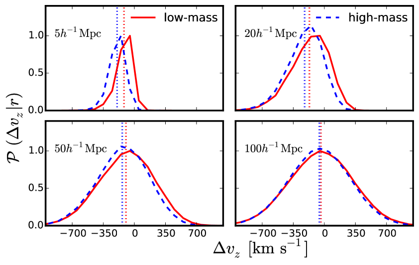
Figure 1: Pairwise line-of-sight velocity PDFs averaged over 160 N-body simulations along the line-of-sight ($0.99\leq\mu\leq 1.0$) for four separations of galaxy pairs: $5.25~{}h^{-1}~{}{\rm Mpc}$ (top left), $20.25~{}h^{-1}~{}{\rm Mpc}$ (top right), $50.25~{}h^{-1}~{}{\rm Mpc}$ (bottom left), and $100.25~{}h^{-1}~{}{\rm Mpc}$ (bottom right). The simulation volume is $(2400~{}h^{-1}~{}{\rm Mpc})^{3}$ and the output is at $z=0$. The red solid and blue dashed lines denote the PDFs for low-mass ($5\times 10^{13}-6.5\times 10^{13}$ $h^{-1}\,M_{\odot}$) and high-mass ($1\times 10^{14}-2.5\times 10^{14}$ $h^{-1}\,M_{\odot}$) halos, for which the average halo biases are $b=1.8$ and 2.5, respectively. Negative (positive) velocities denote galaxy pairs moving towards (away from) each other. The red and blue dashed vertical lines denote the mean pairwise line-of-sight velocity for low-mass and high-mass halos respectively. The PDFs have been normalised to unity, and rescaled such that the maximum of the red lines is unity. For small separations (top panels), there is a small but significant shift towards more negative values for PDFs with a higher mass; for larger separations (bottom panels), the PDFs become more symmetric. However, the mean velocity is still not zero even at separations of $\sim 100h^{-1}\,\rm Mpc$.

Several attempts have been made in the literature [74, 71, 75, 76] to model the redshift-space galaxy two-point correlation function by calculating ${\cal P}(s_{\parallel}-r_{\parallel},\mbox{\boldmath$r$})$ analytically. It is still difficult to predict redshift-space two-point correlation function on all scales without the aid of free parameters. The key issue in modelling the pairwise line-of-sight velocity PDF is its non-Gaussianity; as shown in Ref. [43, 70], the PDF is non-Gaussian even when the density and velocity field follow a Gaussian distribution. As discussed in section 4.3, we also find this non-Gaussianity in the log-normal mock catalogs. The pairwise line-of-sight velocity PDFs that we measure from the log-normal catalogs show qualitatively the same features as those from N-body simulations. In both cases we recover the Kaiser limit on large scales. In section 4.4 we quantitatively discuss how the streaming model reduces to the Kaiser limit at large separations, for our log-normal mocks, making use of the moments of the measured pairwise line-of-sight velocity PDF.

3 Log-normal Catalog Generation

The log-normal distributed density contrast $\delta(\mbox{\boldmath$x$})$ is related to a Gaussian (log-transformed) field $G(\mbox{\boldmath$x$})\equiv\ln\left[1+\delta(\mbox{\boldmath$x$})\right]-\left<\ln\left[1+\delta(\mbox{\boldmath$x$})\right]\right>$ as

$$\delta(\mbox{\boldmath$x$})=e^{-\sigma_{G}^{2}+G(\mbox{\boldmath$x$})}-1\,,$$ (3.1)

where the pre-factor with the variance of the Gaussian field $\sigma_{G}^{2}\equiv\langle G^{2}\rangle$ ensures that the mean of $\delta(\mbox{\boldmath$x$})$ vanishes. Note that the log-normal density fields follow the natural constraint $\delta(\mbox{\boldmath$x$})\geq-1$ of density contrasts by definition. This is not the case for simulations that generate the linear density contrast from Gaussian realisations, although the violation rarely occurs when the variance is small at, e.g., high redshift for setting up the initial conditions of simulations. Applying equation (3.1), one can relate the two-point correlation function of the Gaussian field $\xi^{G}(r)$ to the two-point correlation function of the density field $\xi(r)$ as [33]

$$\xi^{G}(r)=\text{ln}\left[1+\xi(r)\right]\,.$$ (3.2)

Since Gaussian fields of different Fourier modes are uncorrelated, we generate $G$ in Fourier space. To generate a log-normal density field with a given power spectrum $P(k)$, we first Fourier transform the power spectrum to get the target two-point correlation function $\xi(r)$. We then calculate the two-point correlation function of the Gaussian field $\xi^{G}(r)$ by equation (3.2), and Fourier transform $\xi^{G}(r)$ to get the power spectrum $P^{G}(k)$ of $G$. The Fourier space Gaussian field $G(\mbox{\boldmath$k$})$ is generated with [77]

$$G(\mbox{\boldmath$k$})=\sqrt{\frac{P^{G}(k)V}{2}}\left(\theta_{r}+i\theta_{i}\right)\,,$$ (3.3)

where $\theta_{r}$ and $\theta_{i}$ are Gaussian random variables with unit variance and zero mean, and $V$ is the volume of the simulation. We also enforce $G(-\mbox{\boldmath$k$})=G^{*}(\mbox{\boldmath$k$})$ so that the Gaussian field in configuration space $G(\mbox{\boldmath$x$})$ is real. After $G(\mbox{\boldmath$k$})$ is generated at each point in the Fourier grid, we use FFTW library [78] to Fourier-transform $G(\mbox{\boldmath$k$})$ and obtain $G(\mbox{\boldmath$x$})$ on regular cells in configuration space. We then use equation (3.1) to transform $G(\mbox{\boldmath$x$})$ into the desired log-normal density contrast $\delta(\mbox{\boldmath$x$})$ on each cell, with the variance $\sigma_{G}$ measured from $G(\mbox{\boldmath$x$})$ in all cells. The resulting density fluctuation $\delta(\mbox{\boldmath$x$})$ follows a log-normal distribution with the target power spectrum $P(k)$.

At each cell in configuration space, we calculate the expectation value for the number of galaxies $N_{g}(\mbox{\boldmath$x$})=\bar{n}_{g}[1+\delta(\mbox{\boldmath$x$})]V_{\rm cell}$, where $\bar{n}_{g}$ is the global mean galaxy number density and $V_{\rm cell}$ is the volume of the cell. As $N_{g}(\mbox{\boldmath$x$})$ is not an integer, we draw a Poisson random number with the mean $N_{g}(\mbox{\boldmath$x$})$ to obtain the integer number of galaxies in the cell and populate galaxies randomly within the cell. This discretisation is consistent with the nearest-grid-point (NGP) density assignment in the sense that the galaxies are equally spread over the cell.

We next assign velocities to galaxies. For our mock catalogs, we estimate velocities by using the linearised continuity equation of the matter fields:

$$\frac{\partial\delta_{m}(\mbox{\boldmath$x$})}{\partial\eta}+\nabla\cdot\mbox{\boldmath$v$}(\mbox{\boldmath$x$})=0\,,\quad{\rm or}\quad\mbox{\boldmath$v$}(\mbox{\boldmath$k$})=i\mathcal{H}f\frac{\mbox{\boldmath$k$}}{k^{2}}\delta_{m}(\mbox{\boldmath$k$})\,.$$ (3.4)

As the velocity bias can be ignored at the leading order [8], the velocity of a galaxy follows the local matter velocity. We implement this equation as follows. We take the target matter power spectrum to compute $\delta_{m}(\mbox{\boldmath$k$})$ on Fourier cells following the procedures described above, use equation (3.4) to compute $\mbox{\boldmath$v$}(\mbox{\boldmath$k$})$ on each Fourier grid, and then Fourier-transform $\mbox{\boldmath$v$}(\mbox{\boldmath$k$})$ back into configuration space to obtain $\mbox{\boldmath$v$}(\mbox{\boldmath$x$})$ on each cell. To ensure that the galaxy overdensities and velocities are correlated, we use the same random seed for $G$ of galaxies and matter. Namely, the phases of $G_{g}(\mbox{\boldmath$k$})$ and $G_{m}(\mbox{\boldmath$k$})$ are identical; however, this does not imply that the phases of $\delta_{g}(\mbox{\boldmath$k$})$ and $\delta_{m}(\mbox{\boldmath$k$})$ are identical, as we show in section 4.1.2. Finally, we assign the same velocity to all galaxies within one cell.

The target galaxy and matter power spectra can be chosen freely. We need a galaxy bias model [8] to find the matter power spectrum that is consistent with the chosen galaxy power spectrum. In this paper, we use a linear bias relation between the matter and galaxy power spectra, $P_{gg}(k)=b^{2}P_{mm}(k)$, with the linear bias parameter $b$. One important feature of the log-normal catalogs is that even though the target galaxy and matter power spectra are linearly related, the density fields are not proportional to each other (see section 4.1.2). Also, while the galaxy power spectrum and the matter power spectrum are linearly related, the power spectra of their corresponding Gaussian fields are not proportional to each other because

$$\ln[1+b^{2}\xi(r)]\neq b^{2}\ln[1+\xi(r)]\,.$$ (3.5)

We generate 50 log-normal mock catalogs in a cubic volume with $L_{\rm box}=1000~{}h^{-1}~{}{\rm Mpc}$, and $1024^{3}$ grids for the Fourier transformation. This corresponds to the Nyquist frequency of $k_{Ny}=3.22~{}h~{}{\rm Mpc}^{-1}$. The catalogs are generated at $z=1.3$, and each catalog contains roughly 2.1 million galaxies. We compute the input galaxy power spectrum from the linear matter power spectrum using Eisenstein and Hu’s fitting function [79] and the linear galaxy bias $b=1.455$. We assume a flat $\Lambda$CDM model with $\Omega_{m}=0.272$, $n_{s}=0.963$, $A=2.1\times 10^{-9}$. The outcome of this mock generator is a set of positions and velocities of galaxies in three-dimensional space with the target galaxy power spectrum. We shall present detailed tests on the output catalogs in section 4.

4 Validation of the Log-normal Mocks

In this section, we present the results of the log-normal mock generator. We start from the two-point statistics in real space (section 4.1) and then move onto the redshift space correlation function (section 4.2), the pairwise velocity PDF (section 4.3) and recovery of the Kaiser limit on large scales (section 4.4).

4.1 Real-space density statistics

4.1.1 Two-point Statistics

We first measure the real-space two-point statistics: power spectrum and two-point correlation function. As we have pointed out earlier, our log-normal catalogs populate galaxies randomly in each cell, and this is equivalent to adopting the NGP mass assignment scheme. To be consistent, we use NGP with the same grid number to estimate the galaxy density contrast for Fast Fourier Transform (FFT). In this way, we recover the input target power spectrum (having subtracted a constant shot noise $=1/\bar{N}$, $\bar{N}$ denoting the number density of galaxies), without needing to deconvolve the window function due to the density assignment [80]. Should we use a different mesh number or density assignment scheme (such as Cloud-In-Cell), we would have to correct for the window function effects by applying an appropriate deconvolution.

Figure 2 shows the comparison between the input power spectrum and the power spectrum averaged over 50 log-normal realisations (top), and the ratio of the two (bottom). The band shows the error on the mean estimated from 50 realisations. We find an excellent agreement between the measured and input power spectra for $k\lesssim 2~{}h~{}{\rm Mpc}^{-1}$. Note that, when comparing the measurement and prediction we need to take special care to calculate the correct effective wavenumber by which each bin of the measured power spectrum is represented; this is because the binned power spectrum is averaged over many different wavenumbers that fall into the binning criteria. This effect is particularly important on large scales where the number of Fourier modes is small. We present the details of this correction in appendix B.

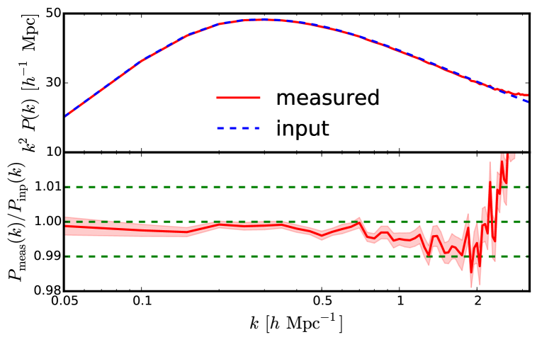
Figure 2: (Top) Mean of the real-space galaxy power spectrum measured from 50 log-normal catalogs (solid) and the input power spectrum (dashed). We show $k^{2}P(k)$. (Bottom) Ratio of the two. The band shows the error on the mean estimated from 50 realisations. The Nyquist frequency for these measurements is $k_{\rm Ny}=3.22\,h$ Mpc^-1.

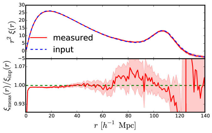
Figure 3: Same as figure 2 but for the correlation function. We show $r^{2}\xi(r)$. The spikes at $r\approx 120-130~{}h^{-1}~{}{\rm Mpc}$ in the bottom panel corresponds to the zero crossing of the correlation function so a small deviation in the mean of the measured correlation function leads to a large ratio. We use a bin size of $1\,h^{-1}$ Mpc.

We measure the galaxy two-point correlation function by using the Landy-Szalay estimator [81]

$$\xi(\mbox{\boldmath$r$})=\frac{DD(\mbox{\boldmath$r$})-2DR(\mbox{\boldmath$r$})+RR(\mbox{\boldmath$r$})}{RR(\mbox{\boldmath$r$})}\,,$$ (4.1)

where $DD(\mbox{\boldmath$r$})$, $DR(\mbox{\boldmath$r$})$, and $RR(\mbox{\boldmath$r$})$ are the number of galaxy-galaxy, galaxy-random, and random-random pairs, respectively. The Landy-Szalay estimator cancels the leading order uncertainties in estimating the mean number density. Figure 3 shows the average of the measured correlation function (top) and the ratio to the input (bottom). We also find an excellent agreement between the measured and input correlation functions over a wide range of scales.

4.1.2 Cross-Correlation Coefficient

We next examine the cross-correlation coefficient

$$r(k)=\frac{P_{gm}(k)}{\sqrt{P_{gg}(k)P_{mm}(k)}}\,,$$ (4.2)

between matter and galaxy density contrasts in real space. Here, $P_{gm}(k)$ denotes the cross power spectrum of galaxy and matter. In figure 5, the red solid line in the top panel shows the measured cross-correlation coefficient $r(k)$ from the log-normal mock catalogs. The measured cross-correlation coefficient approaches unity on large scales, but decreases on small scales with high significance, despite the fact that we have imposed a linear bias relation between the galaxy and matter power spectra, $P_{gg}(k)=b^{2}P_{mm}(k)$, and that the random realisations of $G_{g}$ and $G_{m}$ have been drawn from an identical random seed. This result is a generic feature of log-normal fields that the proportionality relation in power spectra does not guarantee the proportionality of the fields [45]. We can also see this more clearly in a plot of smoothed galaxy and matter density fields, as in figure 4. The smoothed galaxy overdensity deviates significantly from the linearly biased one with $b=1.455$ for all smoothing scales that we chose. In fact, the bias is seen to not even be linear. This is a consequence of the non-linear transformation between the Gaussian and log-normal fields.

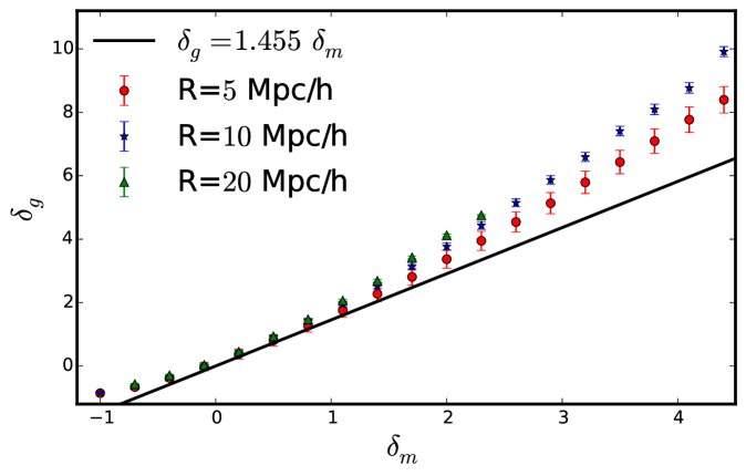
Figure 4: Galaxy overdensity $\delta_{g}$ as a function of matter overdensity $\delta_{m}$ smoothed over different scales - $5\,h^{-1}\rm{Mpc}$ (red circles), $10\,h^{-1}\rm{Mpc}$ (blue stars) and $20\,h^{-1}\rm{Mpc}$ (green triangles). The error bars show the error on the mean of the galaxy overdensity, averaged over all the cells in our 50 mocks.

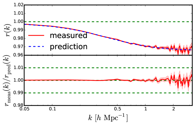
Figure 5: (Top) Measured (red solid) and predicted (blue dashed) cross-correlation coefficient as a function of the wavenumber. The red band shows the error on the mean measured from 50 log-normal mock catalogs. (Bottom) Ratio of the measured to the predicted cross-correlation coefficients.

Because, in our mock, the Gaussian (log-transformed) fields of galaxy and matter have the same random numbers ($\theta_{r}+i\theta_{i}$ in equation (3.3)), they are related to each other in every Fourier cell as

$$\frac{G_{g}(\mbox{\boldmath$k$})}{G_{m}(\mbox{\boldmath$k$})}=\sqrt{\frac{P^{G}_{gg}(k)}{P^{G}_{mm}(k)}}\,,$$ (4.3)

where $P^{G}_{mm}(k)$ and $P^{G}_{gg}(k)$ are the power spectra of $G_{m}$ and $G_{g}$, respectively. Indeed, it is the cross-correlation coefficient between $G_{m}$ and $G_{g}$ that is equal to unity. On the other hand, the galaxy and matter density fields $\delta_{g}(\mbox{\boldmath$x$})$ and $\delta_{m}(\mbox{\boldmath$x$})$ are exponentially related to $G_{g}(\mbox{\boldmath$x$})$ and $G_{m}(\mbox{\boldmath$x$})$. That is, $\delta_{g}(\mbox{\boldmath$k$})$ and $\delta_{m}(\mbox{\boldmath$k$})$ are not linearly related to each other so that the cross-correlation coefficient must deviate from one [45]. On large scales where the correlation functions are small, the cross-correlation approaches unity because $\delta$’s are approximately the same as $G$’s.

We can compute $r(k)$ analytically for log-normal density fields. Specifically, using the one-dimensional Fourier transform we first compute the galaxy-matter cross spectrum as

$$P_{gm}(k)=\int dr~{}r^{2}\xi_{gm}(r)j_{0}(kr)=\int dr~{}r^{2}\left[e^{\xi^{G}_{gm}(r)}-1\right]j_{0}(kr)\,,$$ (4.4)

where $j_{0}(x)$ is the spherical Bessel function of the zeroth order, and $\xi_{gm}({r})=\langle\delta_{g}(\mbox{\boldmath$x$}+\mbox{\boldmath$r$})\delta_{m}(\mbox{\boldmath$x$})\rangle$ and $\xi^{G}_{gm}(r)=\langle G_{g}(\mbox{\boldmath$x$}+\mbox{\boldmath$r$})G_{m}(\mbox{\boldmath$x$})\rangle$. The relation between $\xi_{gm}({r})$ and $\xi^{G}_{gm}(r)$ is analogous to equation (3.2). We then compute $\xi^{G}_{gm}(r)$ as

$$\xi^{G}_{gm}(r)\> =\int\frac{d^{3}k_{1}}{(2\pi)^{3}}\frac{d^{3}k_{2}}{(2\pi)^{3}}\langle{G_{g}(\mbox{\boldmath$k$}_{1})}{G^{*}_{m}(\mbox{\boldmath$k$}_{2})}\rangle e^{i[\mbox{\boldmath$k$}_{1}\cdot(\mbox{\boldmath$x$}+\mbox{\boldmath$r$})-\mbox{\boldmath$k$}_{2}\cdot\mbox{\boldmath$x$}]}$$

$$=\int\frac{d^{3}k_{1}}{(2\pi)^{3}}\frac{d^{3}k_{2}}{(2\pi)^{3}}\sqrt{\frac{P^{G}_{gg}(k_{1})}{P^{G}_{mm}(k_{1})}}\langle{G_{m}(\mbox{\boldmath$k$}_{1})}{G^{*}_{m}(\mbox{\boldmath$k$}_{2})}\rangle e^{i[(\mbox{\boldmath$k$}_{1}-\mbox{\boldmath$k$}_{2})\cdot\mbox{\boldmath$x$}+\mbox{\boldmath$k$}_{1}\cdot\mbox{\boldmath$r$}]}$$

$$=\int\frac{dk}{2\pi^{2}}k^{2}\sqrt{P^{G}_{gg}(k)P^{G}_{mm}(k)}j_{0}(kr)\,.$$ (4.5)

Combining equations (4.4)–(4.5), $r(k)$ can be evaluated. The blue dashed line in the top panel of figure 5 shows the prediction, whereas the bottom panel shows the ratio between the measurement and the prediction. We find an excellent agreement between the measurement and the prediction.

4.2 Redshift-space density statistics

We now present the measurements of the two-point statistics in redshift space. We obtain the redshift-space mock catalogs from the real-space ones by mapping real-space positions of galaxies to redshift-space positions by equation (2.1). We use the periodic boundary condition along the $z$-direction for galaxies that move out of the box by this mapping. Measurements of the power spectrum or correlation function for these redshift-space catalogs proceed in the same manner as in real space.

As described in section 2, when linearising the Jacobian, the redshift-space power spectrum is given by

$$P^{s}_{gg}(k,\mu_{k})=P_{gg}(k)+2\mu_{k}^{2}fP_{gm}(k)+\mu_{k}^{4}f^{2}P_{mm}(k).$$ (4.6)

When using linear theory (that we shall call “Kaiser”), we relate the galaxy-galaxy power spectrum and galaxy-matter power spectrum to the matter-matter power spectrum as $P_{gg}(k)=b^{2}P_{mm}(k)$ and $P_{gm}(k)=bP_{mm}(k)$. We stress, however, that the galaxy-matter cross power spectrum $P_{gm}(k)$ is not equal to $bP_{mm}(k)$ for the log-normal density fields, as shown in section 4.1.2. Therefore, in order to highlight the effect from non-linearity in the Jacobian, we calculate the redshift-space galaxy power spectrum with equation (4.6) but use the cross power spectrum in section 4.1.2 (that we call “linear Jacobian”).

Figures (6)–(7) show the measured monopole and quadrupole power spectra, compared with the Kaiser (with $P_{gm}(k)=bP_{mm}(k)$) and the linear Jacobian (with measured $P_{gm}(k)$) predictions. On large scales (small $k$), we find a good agreement for all three cases as expected. On small scales, the linear Jacobian calculation deviates from the Kaiser value due to the non-unity cross-correlation between the matter and galaxy (section 4.1.2). The deviation is smaller than what we find in figure 5 because $f/b=0.616$ is less than unity.

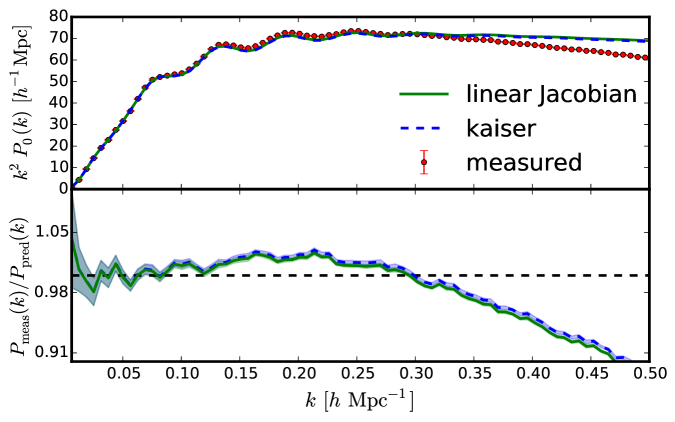
Figure 6: (Top) Monopole redshift-space power spectrum. The red points show the measurement averaged over 50 log-normal mock catalogs. The blue dashed line shows the Kaiser prediction while the green solid line shows the linear Jacobian prediction. We show $k^{2}P_{0}(k)$ to enhance differences at large $k$. (Bottom) Ratio of the measured monopole power to the Kaiser and linear Jacobian predictions. The band shows the error on the mean estimated from 50 realisations. We find a sub-1% agreement on scales $k\apprle 0.1~{}h~{}{\rm Mpc}^{-1}$.

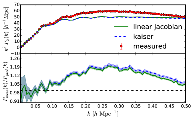
Figure 7: Same as figure 6, but for the quadrupole power spectrum.

Both the Kaiser and linear Jacobian calculations fail to model the measured monopole and quadrupole power spectra on small scales. As we use the real-space power spectrum used to generate the log-normal catalog in each term in equation (4.6), any discrepancy that we find in figures (6)–(7) is due to non-linearity in the mapping between real and redshift space. That is, when densities and velocities become large, the Jacobian cannot be linearised, and so the linear Jacobian approximation is no longer valid. For example, the measured monopole power spectrum in figure 6 is smaller than the linear Jacobian calculation on small scales ($k>0.3\,h\,{\rm Mpc}^{-1}$). This behaviour is qualitatively similar to the FoG damping effect, which is usually attributed to RSD of random motion within bigger halos. In our log-normal mock catalog, however, the damping cannot be the FoG effect because we do not include any random component when generating peculiar velocities. Rather, the power suppression we see here originates solely from non-linearity in the Jacobian of real-to-redshift mapping due to coherent peculiar velocity fields given by the continuity equation.

Mathematically, combining equations (2.3)–(2.4) yields the the non-linear mapping between the real- and redshift-space density contrasts

$$1+\delta^{s}_{g}(\mbox{\boldmath$s$})=\frac{1+\delta_{g}(\mbox{\boldmath$x$})}{\left|1+\frac{1}{\mathcal{H}}\frac{\partial v_{z}(\mbox{\boldmath$x$})}{\partial z}\right|}\,,$$ (4.7)

which turns to, in Fourier space [66],

$$\delta^{s}_{g}(\mbox{\boldmath$k$})=\int d^{3}x\,e^{-i\mbox{\boldmath$k$}\cdot\mbox{\boldmath$x$}}\left[\delta_{g}(\mbox{\boldmath$x$})-\frac{1}{\mathcal{H}}\frac{\partial v_{z}(\mbox{\boldmath$x$})}{\partial z}\right]e^{ik_{z}v_{z}(\mbox{\boldmath$x$})/\mathcal{H}}\,.$$ (4.8)

As long as velocities are small, i.e. $k_{z}v_{z}\ll 1$, the exponential factor in equation (4.8) can be approximated to unity, leading to the linear Jacobian formula. However, on small scales, this approximation breaks down, and the exponential factor leads to the non-linear Jacobian effects [66].

We show the configuration-space two-point correlation function in figures (8)–(9), and compare them with the linearised Jacobian prediction:

$$\delta_{g}^{s}(\mbox{\boldmath$s$})=\delta_{g}(\mbox{\boldmath$x$})-\frac{1}{{\cal H}}\frac{\partial}{\partial z}v_{z}(\mbox{\boldmath$x$})\,.$$ (4.9)

Combining with the linear continuity equation that we use to generate the velocity field,

$$\mbox{\boldmath$v$}(\mbox{\boldmath$x$})=-{\cal H}f\nabla\left[\nabla^{-2}\delta_{m}(\mbox{\boldmath$x$})\right],$$ (4.10)

we find the configuration space expression for the redshift-space density contrast:

$$\delta_{g}^{s}(\mbox{\boldmath$s$})=\delta_{g}+f\left(\frac{\partial}{\partial z}\right)^{2}\left[\nabla^{-2}\delta_{m}(\mbox{\boldmath$x$})\right],$$ (4.11)

from which we calculate

$$\xi^{s}_{gg}(s,\mu)\> =\left[\xi_{gg}(s)+\frac{2}{3}f\xi_{gm}(s)+\frac{1}{5}f^{2}\xi_{mm}(s)\right]$$

$$-\left[\frac{4}{3}f\xi_{gm,2}(s)+\frac{4}{7}f^{2}\xi_{mm,2}(s)\right]{\cal L}_{2}(\mu)+\frac{8}{35}f^{2}\xi_{mm,4}(s){\cal L}_{4}(\mu).$$ (4.12)

Just like the case for the power spectrum, the expression reduces to the linear Kaiser prediction (equation (2.12)) when we set $\xi_{gm}(r)=b\xi_{mm}(r)$, but we must take into account non-unity cross-correlation function for the log-normal catalog.

While the Kaiser and linear Jacobian models are reproduced in the power spectrum at $k\lesssim 0.1~{}h~{}{\rm Mpc}^{-1}$, they are not well reproduced in the correlation functions at all separations. This indicates that the correlation functions at large separations are sensitive to non-linearity in the Jacobian.

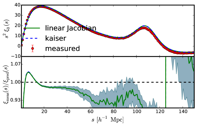
Figure 8: (Top) Monopole redshift-space two-point correlation function. The meaning of the lines is the same as in figure 6. We show $s^{2}\xi_{0}(s)$ to enhance differences on large separations. (Bottom) Ratio of the measured monopole correlation function to the Kaiser and linear Jacobian predictions. The Kaiser and linear Jacobian predictions lie almost on top of each other, and so are hard to distinguish.

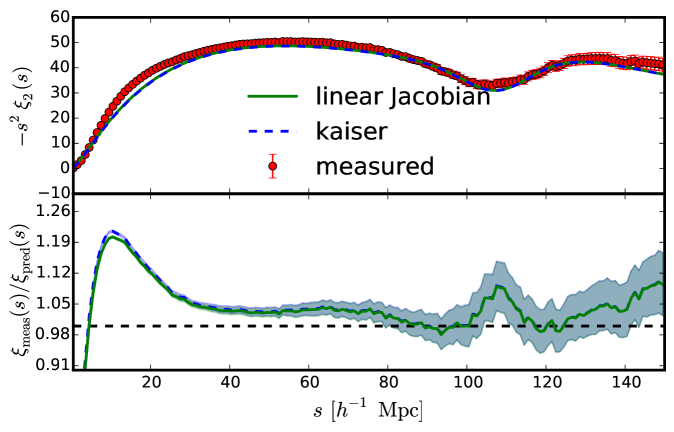
Figure 9: Same as figure 8, but for the quadrupole two-point correlation function. We show $-s^{2}\xi_{2}(s)$.

4.3 Pairwise Line-of-Sight Velocity PDFs

How do we incorporate non-linearity in the Jacobian into the model? As discussed in section 2, the pairwise line-of-sight velocity PDF fully describes the mapping from the real-space two-point correlation function to the redshift-space one.

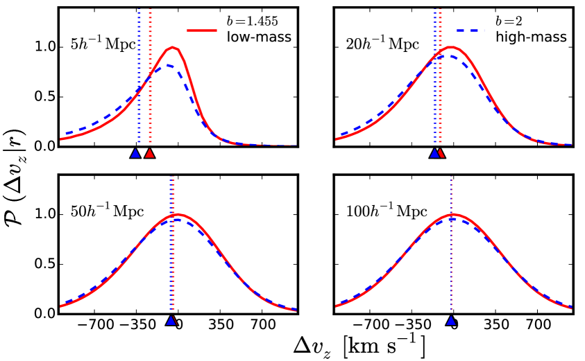
Figure 10: Same as figure 1, but for PDFs averaged over 50 log-normal mock catalogs. The simulation volume is $(1000~{}h^{-1}~{}{\rm Mpc})^{3}$ and the output is at $z=1.3$. The biases of low- and high-mass catalogs are $b=1.455$ (red) and 2 (blue), respectively. The triangles on the horizontal axes show the calculations from equation (4.14).

We show in figure 10 the PDFs of pairwise line-of-sight velocity averaged over 50 log-normal mock catalogs, for four different separations between galaxy pairs (From top left to bottom right, $5.25$, $20.25$, $50.25$, and $100.25~{}h^{-1}~{}{\rm Mpc}$) along the line-of-sight direction ($0.99\leq\mu\leq 1$). We show the pairwise line-of-sight velocity PDFs along the line-of-sight direction because the relative peculiar velocities are at their maximum (i.e., no perpendicular component). For the streaming model, we need the relative velocity PDFs for galaxy pairs along all directions.

We show the measured pairwise line-of-sight velocity PDFs for two different linear biases $b=1.455$ (low-mass) and 2 (high-mass) as, respectively, the blue dashed lines and the red solid lines. Note that we use the same phases (that is, the same sequence of random numbers) for generating velocity fields for both cases; thus, galaxies in the same cell have identical velocities regardless of the assumed bias parameter. Overall, we find that the pairwise line-of-sight velocity PDFs from our log-normal mock catalogs capture qualitative features that we have seen in N-body simulations (figure 1). Namely, both PDFs have negative mean velocity and negative skewness for smaller separations (top panels of figure 10 and figure 1) and approach a symmetric PDF for larger separations. Also, the tendency is more obvious for high-mass (high-bias) galaxies. The log-normal catalogs show larger velocity dispersion than N-body simulations especially at small separations.

Our results show that the coherent irrotational velocity given by the linearised continuity equation can explain a part of the non-linear features in the pairwise line-of-sight velocity PDF. We stress, again, that we do not include any random velocities. Also note that we have assigned the same velocity to all galaxies in the same cell, and the velocity field is exactly the same for the high-mass and low-mass samples. Nevertheless, the pairwise line-of-sight velocity PDF for galaxies with different biases are still different due to pair weighting: velocities of galaxies with high (low) bias are weighted higher (lower) density regions.

While successful at a qualitative level, the PDFs from log-normal catalogs and those from N-body simulations are different in detail. For example, the velocity field in our log-normal mock catalogs only reflects non-Gaussianity of the log-normal density fields, which is not the same as that in N-body simulations where the complete non-linear gravitational evolution is encoded.

Strong non-Gaussianity in the pairwise line-of-sight velocity PDF makes it challenging to analytically compute its full moments, even if the velocity field is assumed to follow the linear continuity equation. Nevertheless, we can still compute the mean pairwise line-of-sight velocity (that is, the first moment) as follows. Using the linearised continuity equation (equation (2.7)), the parallel component of relative velocity for galaxies separated by $r$ is given by

$$v_{1z}-v_{2z}=i\mathcal{H}f\int\frac{d^{3}k}{(2\pi)^{3}}\frac{k_{z}}{k^{2}}\delta_{m}(\mbox{\boldmath$k$})\left(e^{i\mbox{\boldmath$k$}\cdot\mbox{\boldmath$x$}_{1}}-e^{i\mbox{\boldmath$k$}\cdot\mbox{\boldmath$x$}_{2}}\right)\,.$$ (4.13)

Because the parallel relative velocity is the exponent in the velocity generating function (equation (2.14)), the mean pairwise line-of-sight velocity can be calculated from

$$\langle\Delta v_{z}\rangle={\cal H}\left.\frac{\partial M(\lambda,\mbox{\boldmath$r$})}{\partial\lambda}\right|_{\lambda=0}\> =\frac{\left\langle\left(v_{1z}-v_{2z}\right)\left[1+\delta_{g1}\right]\left[1+\delta_{g2}\right]\right\rangle}{1+\xi_{gg}(r)}$$

$$=i\mathcal{H}f\frac{\int d^{3}x^{\prime}q(\mbox{\boldmath$x$}^{\prime}_{1},\mbox{\boldmath$x$}^{\prime}_{2})\left\langle\left[1+\delta_{g1}\right]\left[1+\delta_{g2}\right]\delta_{m3}\right\rangle}{1+\xi_{gg}(r)}\,,$$ (4.14)

where $\mbox{\boldmath$x$}^{\prime}_{i}\equiv\mbox{\boldmath$x$}_{i}-\mbox{\boldmath$x$}^{\prime}$, $\delta_{m3}=\delta_{m}(\mbox{\boldmath$x$}^{\prime})$, and

$$q(\mbox{\boldmath$x$}^{\prime}_{1},\mbox{\boldmath$x$}^{\prime}_{2})\equiv\int\frac{d^{3}k}{(2\pi)^{3}}\frac{k_{z}}{k^{2}}\left(e^{i\mbox{\boldmath$k$}\cdot\mbox{\boldmath$x$}^{\prime}_{1}}-e^{i\mbox{\boldmath$k$}\cdot\mbox{\boldmath$x$}^{\prime}_{2}}\right)\,.$$ (4.15)

The triangles on the horizontal axes in figure 10 show the predictions computed from equation (4.14). We find that they are in an excellent agreement with the measurements. As shown in equation (4.14) the mean of the pairwise line-of-sight velocity depends on the integral of the three-point function of the log-normal fields. We present the details of this calculation in appendix C.

Likewise, in order to compute the $n$th-order moments of the pairwise line-of-sight velocity we need to integrate over $(n+2)$-point correlation functions of the log-normal fields. Thus, it is impractical to compute all the moments of the pairwise line-of-sight velocity PDF, even though the statistics of log-normal fields are known. On the other hand, should we assume a Gaussian PDF for the pairwise line-of-sight velocity distribution, all the higher-order moments but the first two would be ignored; thus, we miss the non-Gaussian effects coming from non-linear evolution of the Universe as well as the pair weighting effect.

4.4 Recovery of Kaiser limit

Even though the pairwise velocity PDF in our log-normal mocks does not precisely reproduce the velocity PDF from N-body simulations (see for example, figure 11, for a comparison of the first two moments of the pairwise velocities as a function of separation), the redshift space power spectrum from both matches the Kaiser prediction on large scales ($k\lesssim 0.1\,h$ Mpc^-1). To understand why this happens, we now consider the redshift space two-point correlation function in the large-scale limit, i.e. separations such that only the linear order terms contribute.

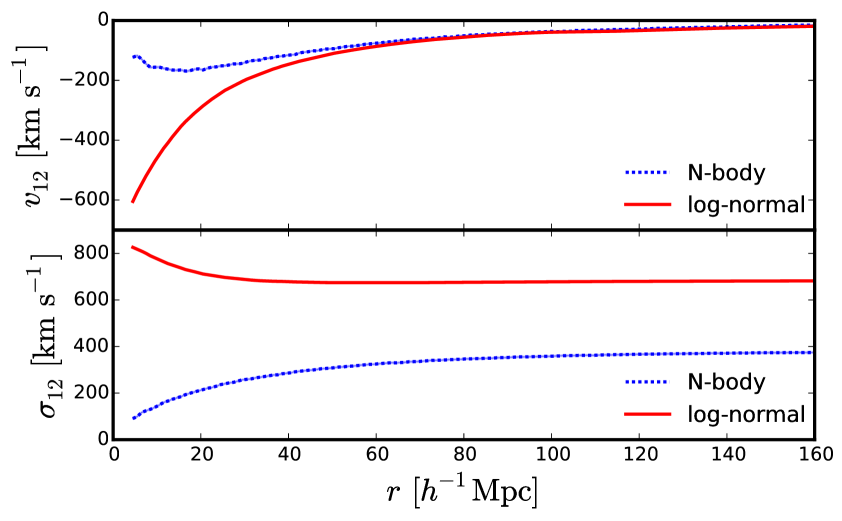
Figure 11: Mean (top) and dispersion (bottom) of pairwise velocity from log-normal mocks (red) and N-body simulations (blue) as a function of pair separation $r$, for pairs along the line-of-sight, $0.99\leq\mu\leq 1.0$. The linear bias for log-normal mocks was chosen to be $b=1.8$ which is the average linear bias for the halos in the mass range $5\times 10^{13}-6.5\times 10^{13}$ $h^{-1}\,M_{\odot}$ shown above.

The large-scale limit of the redshift space two-point correlation function (to linear order) is given as [70]

$$\xi^{s}_{gg}(s_{\parallel},s_{\perp})=\xi_{gg}(s)-\frac{{\rm d}}{{\rm d}r_{\parallel}}\Big{[}v_{12}(r)\frac{r_{\parallel}}{r}\Big{]}\Big{|}_{r_{\parallel}=s_{\parallel}}+\frac{1}{2}\frac{{\rm d}^{2}}{{\rm d}r_{\parallel}^{2}}\Big{[}\sigma^{2}_{12}(r,\mu)\Big{]}\Big{|}_{r_{\parallel}=s_{\parallel}}\,,$$ (4.16)

where $s^{2}\equiv s^{2}_{\parallel}+s^{2}_{\perp}$, $r^{2}\equiv s^{2}_{\perp}+r_{\parallel}^{2}$, $v_{12}(r)$ is the mean of the radial pairwise velocity (which is the relative velocity projected along the line joining the pair of particles; we call the remaining component tangential pairwise velocity), and $\sigma^{2}_{12}(r,\mu)$ is the variance of the line-of-sight pairwise velocities, with $\mu\equiv r_{\parallel}/r$.

In linear theory, the mean and variance can be calculated as

$$v_{12}(r) =-\frac{\mathcal{H}fb}{\pi^{2}}\int dkkP_{\rm mm}(k)j_{1}(kr)\,,$$ (4.17)

$$\sigma^{2}_{12}(r,\mu) =2[\sigma^{2}_{v}-\mu^{2}\Psi_{\parallel}-(1-\mu^{2})\Psi_{\perp}]\,,$$ (4.18)

$$\Psi_{\parallel}(r) =\frac{\mathcal{H}^{2}f^{2}}{2\pi^{2}}\int dkP_{\rm mm}(k)\Bigg{[}j_{0}(kr)-\frac{2j_{1}(kr)}{kr}\Bigg{]}\,,$$ (4.19)

$$\Psi_{\perp}(r) =\frac{\mathcal{H}^{2}f^{2}}{2\pi^{2}}\int dkP_{\rm mm}(k)\frac{j_{1}(kr)}{kr}\,,$$ (4.20)

where $\sigma^{2}_{v}\equiv\left\langle\mbox{\boldmath$v$}(\mbox{\boldmath$x$})\cdot\mbox{\boldmath$v$}(\mbox{\boldmath$x$})\right\rangle/3$ is the one-dimensional velocity variance, $P_{\rm mm}(k)$ is the matter power spectrum in real space, $\Psi_{\parallel}$ is the variance of the radial pairwise velocities, $\Psi_{\perp}$ is the variance of the tangential pairwise velocities, and $j_{n}$ denotes the spherical Bessel function of the $n^{\rm th}$ order. As shown in refs. [70, 76],

$$-\frac{{\rm d}}{{\rm d}r_{\parallel}}\Big{[}v_{12}(r)\frac{r_{\parallel}}{r}\Big{]}\Big{|}_{r_{\parallel}=s_{\parallel}} =\frac{v_{12}(r)}{r}(\mu^{2}-1)-v^{\prime}_{12}(r)\mu^{2}\,,$$ (4.21)

$$\frac{1}{2}\frac{{\rm d}^{2}}{{\rm d}r_{\parallel}^{2}}\Big{[}\sigma^{2}_{12}(r,\mu)\Big{]}\Big{|}_{r_{\parallel}=s_{\parallel}} =(2-10\mu^{2}+8\mu^{4})\frac{\Psi_{\perp}-\Psi_{\parallel}}{r^{2}}+(5\mu^{4}-5\mu^{2})\frac{\Psi^{\prime}_{\parallel}}{r}$$

$$+(-1+6\mu^{2}-5\mu^{4})\frac{\Psi^{\prime}_{\perp}}{r}-\mu^{4}\Psi^{\prime\prime}_{\parallel}+(\mu^{4}-\mu^{2})\Psi^{\prime\prime}_{\perp}\,,$$ (4.22)

so that the Kaiser limit of the redshift space two-point correlation function does not depend on any constant or the isotropic dispersion of the pairwise line-of-sight velocities. In this section ^′ denotes $d/dr$.

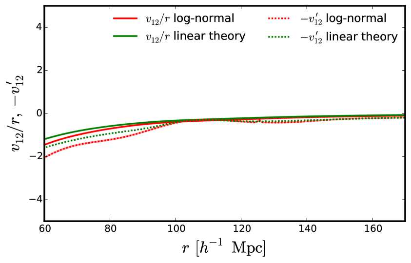
Figure 12: Mean radial pairwise velocity (solid) measured from our log-normal mocks (red) as well as that predicted by linear theory (green). Derivative w.r.t. separation $r$ (dotted). Red band denotes the error on the mean measured from 50 realisations. They agree at separations $\gtrsim 140\,h^{-1}$ Mpc.

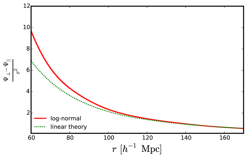
Figure 13: Same as figure 12 but for difference of radial ($\Psi_{\parallel}$) and tangential ($\Psi_{\perp}$) pairwise velocity variances. They agree at separations $\gtrsim 140\,h^{-1}$ Mpc.

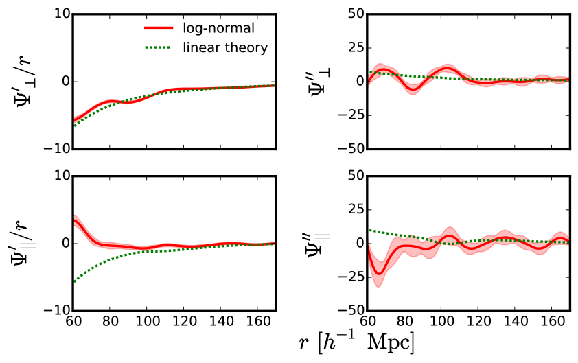
Figure 14: Same as figure 12 but for first and second derivatives of tangential and radial pairwise velocity variances. The second derivatives are noisy but they seem to agree with linear theory predictions at separations $\gtrsim 120\,h^{-1}$ Mpc.

In figures (12)–(14) we show the different terms that contribute to the Kaiser limit of the two-point correlation function, namely, $v_{12}/r$, $v^{\prime}_{12}$, $(\Psi_{\perp}-\Psi_{\parallel})/r^{2}$, $\Psi^{\prime}_{\parallel}/r$, $\Psi^{\prime}_{\perp}/r$, $\Psi^{\prime\prime}_{\parallel}$, and $\Psi^{\prime\prime}_{\perp}$ for our log-normal mocks (run to match the conditions from the N-body simulations, i.e. we choose $b=1.8$ which is the average linear bias for halos in the mass range $5\times 10^{13}-6.5\times 10^{13}$ $h^{-1}\,M_{\odot}$ at $z=0$) and linear theory predictions. They agree at large separations, which ensures that the Kaiser limit is attained. This is because only the spatial derivatives of the first two moments of the pairwise velocity PDF contribute to the lowest-order redshift space correlation function in the large-scale limit [70, 43, 76], as we confirm. So, even though the PDF from our log-normal mocks shows a non-zero excess kurtosis on large scales (which is a consequence of the non-zero excess kurtosis of the log-normal density PDF, as only the one-point distribution is relevant for large separations) and the dispersion is larger than the one from the N-body simulations (by a scale-independent constant), we find agreement with the Kaiser prediction on large scales.

5 Summary and Conclusions

We have presented a new public code for generating log-normal realisations including velocity fields satisfying the linear continuity equation. The log-normal realisations provide not only a fast and easy way to generate mock galaxy catalogs but also an excellent test bed for studying non-linear effects such as the window function and RSD.

We have verified that the real-space two-point correlation functions measured from our log-normal mock galaxy catalogs are in excellent agreement with the input. We find that the cross-correlation coefficients between the matter and galaxy density fields are not unity [45]. Non-linear (exponential, to be specific) transformation of perfectly correlated Gaussian fields induces a deviation of the cross-correlation coefficient from unity. We analytically compute the cross-correlation coefficient that matches the measurement to a sub-percent level.

We have also shown measurements from our log-normal mock catalogs in redshift space. The redshift-space power spectrum is commonly modelled as a combination of a “squashing” term (in the Kaiser limit, arising from coherent large-scale flows) and a damping term (FoG from random virial motion on small scales). Using our log-normal mock catalogs, we have investigated the redshift-space power spectrum and found a good agreement with the squashing term on large scales ($k\apprle 0.1\,h^{-1}$ Mpc) as expected. On small scales, we find a damping which is qualitatively similar to the FoG; the damping we observe, however, does not come from random motion, as we do not include any random virial motion in our mock generator. Rather, the damping comes from non-linearity in the Jacobian of the real-to-redshift space mapping, and from the coherent peculiar velocity field. Attributing all of the damping to the FoG, as commonly done in the literature, is thus misleading. The configuration space two-point correlation function calculated with the linear Jacobian approximation cannot reproduce the measurement at all separations; thus, the correlation function is sensitive to non-linearity in the Jacobian even at large separations.

The streaming model can take into account the full non-linearity of the real-to-redshift space mapping. In this model a fundamental entity in predicting the redshift-space two-point statistics is the pairwise line-of-sight velocity PDF, which is notoriously hard to predict owing to its pairwise nature. We find that the problem persists even with our, rather simpler, setting: the PDF of the density field is exactly known to be log-normal, and the velocity is linearly related to the density field. We nevertheless have made some progress in a couple of areas in modelling the pairwise line-of-sight velocity PDF. First, we show that the pairwise line-of-sight velocity PDF from our log-normal mock catalogs qualitatively captures features of the PDF from full N-body simulations, such as a negative skewness for small separations and the shift of the PDF towards more negative velocities for higher mass halos. We find these features even when the same coherent velocity field is assigned to galaxy fields with different biases, i.e., galaxies with different biases move with the same velocities, but pair-weighting makes the pairwise velocity PDF depend on the galaxy bias. Second, for the log-normal setting, one can in principle predict the moments of the pairwise line-of-sight velocity PDF, as we explicitly demonstrate for the mean pairwise line-of-sight velocity. We have compared the predicted mean velocity to the one measured from the catalogs, and find an excellent match between the two. Likewise, although very demanding, we envisage that the analytical calculation can also be done for the higher order moments.

Our log-normal generator has been used extensively to help design the on-going and planned galaxy redshift surveys such as HETDEX (Hobby-Eberly Telescope Dark Energy Experiment) [82], PFS (Prime Focus Spectrograph) [83], and WFIRST-AFTA (Wide Field Infrared Survey Telescope Astrophysics-Focused Telescope Assets) [84]. It should also be equally useful for DESI (Dark Energy Spectroscopic Instrument) [85], LSST (Large Synoptic Survey Telescope) [86], and Euclid [87]. In near future we shall make available a code for computing weak gravitational lensing fields from the log-normal density field (“log-normal_lens”; Makiya et al., in preparation). This code allows us to study the cross-correlation power spectrum between galaxy positions and weak lensing fields, which is one of the products of PFS and Euclid as well as LSST with spectroscopic follow-ups.

Appendix A Derivation of the streaming model in configuration space

In this appendix, we re-derive the streaming model [68, 69, 70, 43, 71], which equates the redshift-space two-point correlation function $\xi_{gg}^{s}$ to the real-space two-point correlation function $\xi_{gg}$ re-mapped by the pairwise line-of-sight velocity PDF ${\cal P}$ as

$$1+\xi_{gg}^{s}(\mbox{\boldmath$s$})=\int dr_{\parallel}{\cal P}\left(s_{\parallel}-r_{\parallel};\mbox{\boldmath$r$}\right)\left[1+\xi_{gg}(\mbox{\boldmath$r$})\right]\,.$$ (A.1)

Here, $s$ and $r$ are, respectively, the separations in redshift space and real space. To the best of our knowledge, the streaming model in the form of equation (A.1) has first appeared in [68], and the later studies [69, 70, 43, 71] have improved the modelling and interpretation of the pairwise line-of-sight velocity PDF. For example, Ref. [70] incorporates the scale-dependence of the velocity dispersion to reproduce the Kaiser [48] prediction; Ref. [43] finds the expression for the pairwise line-of-sight velocity PDF and its moment generating function with an assumption that the velocity field $\mbox{\boldmath$v$}(\mbox{\boldmath$r$})$ is a single-valued function of positions (we shall call this single-stream case). More recently, Ref. [71] generalizes the results to the multi-stream case where there are multiple velocity components (streams) at a single position; this is, for example, the case for the shell crossing in the spherical collapse. Here, we shall closely follow the result of Ref. [71] so that derivation we present here works for the multi-streaming case.

Starting from the galaxy number conservation between the real and redshift space (equation (2.2)), and using the general phase space function $f(\mbox{\boldmath$x$},\mbox{\boldmath$v$})$, we may write the redshift-space density contrast as [60]:

$$1+\delta_{g}^{s}(\mbox{\boldmath$s$})=\int d^{3}x\int d^{3}v~{}f(\mbox{\boldmath$x$},\mbox{\boldmath$v$})\delta^{D}\left(\mbox{\boldmath$x$}+\frac{v_{\parallel}}{{\cal H}}\hat{\ell}-\mbox{\boldmath$s$}\right),$$ (A.2)

where $\delta^{D}$ is the Dirac-delta operator. The redshift-space two-point correlation function is then given as

$$\,\left<\left[1+\delta_{g}^{s}(\mbox{\boldmath$s$}_{1})\right]\left[1+\delta_{g}^{s}(\mbox{\boldmath$s$}_{2})\right]\right>=\int d^{3}\mbox{\boldmath$x$}_{1}\int d^{3}\mbox{\boldmath$x$}_{2}\int d^{3}\mbox{\boldmath$v$}_{1}\int d^{3}\mbox{\boldmath$v$}_{2}$$

$$\,\left<\delta^{D}\left(\mbox{\boldmath$x$}_{1}-\mbox{\boldmath$s$}_{1}+\frac{v_{1,\parallel}}{{\cal H}}\hat{\ell}\right)\delta^{D}\left(\mbox{\boldmath$x$}_{2}-\mbox{\boldmath$s$}_{2}+\frac{v_{2,\parallel}}{{\cal H}}\hat{\ell}\right)f(\mbox{\boldmath$x$}_{1},\mbox{\boldmath$v$}_{1})f(\mbox{\boldmath$x$}_{2},\mbox{\boldmath$v$}_{2})\right>.$$ (A.3)

As is apparent from equation (2.1), the RSD only applies to the line-of-sight quantities, so it is helpful to explicitly indicate the line-of-sight quantities with the subscript $\parallel$ and perpendicular quantities with the subscript $\perp$. Then, equation (A.3) becomes

$$\left<\left[1+\delta_{g}^{s}\left(s_{1,\parallel},s_{1,\perp}\right)\right]\left[1+\delta_{g}^{s}\left(s_{2,\parallel},s_{2,\perp}\right)\right]\right>=\int dx_{1,\parallel}\int dx_{2,\parallel}\int d^{3}\mbox{\boldmath$v$}_{1}\int d^{3}\mbox{\boldmath$v$}_{2}$$

$$\left<\delta^{D}\left(x_{1,\parallel}-s_{1,\parallel}+\frac{v_{1,\parallel}}{{\cal H}}\right)\delta^{D}\left(x_{2,\parallel}-s_{2,\parallel}+\frac{v_{2,\parallel}}{{\cal H}}\right)f(x_{1,\parallel},s_{1,\perp},\mbox{\boldmath$v$}_{1})f(x_{2,\parallel},s_{2,\perp},\mbox{\boldmath$v$}_{2})\right>\,.$$ (A.4)

Here, we keep the Dirac-delta operators inside the ensemble average as they contain the peculiar velocity field. We then use the definition of the Dirac-delta $\delta^{D}(x)=(2\pi)^{-1}\int_{-\infty}^{\infty}d\gamma e^{-i\gamma x}$, to transform equation (A.4) as

$$\left<\left[1+\delta_{g}^{s}\left(s_{1,\parallel},s_{1,\perp}\right)\right]\left[1+\delta_{g}^{s}\left(s_{2,\parallel},s_{2,\perp}\right)\right]\right>=\int dx_{1,\parallel}\int dx_{2,\parallel}\int\frac{d\gamma_{1}}{2\pi}\int\frac{d\gamma_{2}}{2\pi}e^{-i\gamma_{1}\left(x_{1,\parallel}-s_{1,\parallel}\right)}$$

$$e^{-i\gamma_{2}\left(x_{2,\parallel}-s_{2,\parallel}\right)}\times\int d^{3}\mbox{\boldmath$v$}_{1}\int d^{3}\mbox{\boldmath$v$}_{2}\left<e^{-i\gamma_{1}\frac{v_{1,\parallel}}{{\cal H}}}e^{-i\gamma_{2}\frac{v_{2,\parallel}}{{\cal H}}}f(x_{1,\parallel},s_{1,\perp},\mbox{\boldmath$v$}_{1})f(x_{2,\parallel},s_{2,\perp},\mbox{\boldmath$v$}_{2})\right>.$$ (A.5)

Because of statistical homogeneity of the Universe, the ensemble average must depend only on the separation. We make it explicit by introducing new variables $R_{\parallel}=(x_{1,\parallel}+x_{2,\parallel})/2$ and $r_{\parallel}=x_{1,\parallel}-x_{2,\parallel}$, with which the right-hand side of the equation above becomes

$$\,\left<\left[1+\delta_{g}^{s}\left(s_{1,\parallel},s_{1,\perp}\right)\right]\left[1+\delta_{g}^{s}\left(s_{2,\parallel},s_{2,\perp}\right)\right]\right>$$

$$= \,\int dr_{\parallel}\int\frac{d\gamma_{1}}{2\pi}\int d\gamma_{2}\left[\int\frac{dR_{\parallel}}{2\pi}e^{-iR_{\parallel}\left(\gamma_{1}+\gamma_{2}\right)}\right]e^{-\frac{i}{2}r_{\parallel}\left(\gamma_{1}-\gamma_{2}\right)}e^{i\left(\gamma_{1}s_{1,\parallel}+\gamma_{2}s_{2,\parallel}\right)}$$

$$\times\int d^{3}\mbox{\boldmath$v$}_{1}\int d^{3}\mbox{\boldmath$v$}_{2}\left<e^{-i\gamma_{1}\frac{v_{1,\parallel}}{{\cal H}}}e^{-i\gamma_{2}\frac{v_{2,\parallel}}{{\cal H}}}f(x_{1,\parallel},s_{1,\perp},\mbox{\boldmath$v$}_{1})f(x_{2,\parallel},s_{2,\perp},\mbox{\boldmath$v$}_{2})\right>$$

$$= \,\int dr_{\parallel}\int\frac{d\gamma_{1}}{2\pi}\int d\gamma_{2}\delta^{D}(\gamma_{1}+\gamma_{2})e^{-\frac{i}{2}r_{\parallel}\left(\gamma_{1}-\gamma_{2}\right)}e^{i\left(\gamma_{1}s_{1,\parallel}+\gamma_{2}s_{2,\parallel}\right)}$$

$$\times\int d^{3}\mbox{\boldmath$v$}_{1}\int d^{3}\mbox{\boldmath$v$}_{2}\left<e^{-i\gamma_{1}\frac{v_{1,\parallel}}{{\cal H}}}e^{-i\gamma_{2}\frac{v_{2,\parallel}}{{\cal H}}}f(x_{1,\parallel},s_{1,\perp},\mbox{\boldmath$v$}_{1})f(x_{2,\parallel},s_{2,\perp},\mbox{\boldmath$v$}_{2})\right>\,.$$ (A.6)

Finally, integrating the Dirac-delta yields

$$1+\xi_{gg}^{s}(s_{\parallel},s_{\perp})= \,\int dr_{\parallel}\int\frac{d\gamma_{1}}{2\pi}e^{-i\gamma_{1}(r_{\parallel}-s_{\parallel})}\int d^{3}\mbox{\boldmath$v$}_{1}\int d^{3}\mbox{\boldmath$v$}_{2}\left<e^{-i\gamma_{1}\frac{\Delta v_{\parallel}}{{\cal H}}}f(x_{1,\parallel},s_{1,\perp},\mbox{\boldmath$v$}_{1})f(x_{2,\parallel},s_{2,\perp},\mbox{\boldmath$v$}_{2})\right>\,,$$ (A.7)

with $\Delta v_{\parallel}=v_{1,\parallel}-v_{2,\parallel}$. Again, note that the ensemble average must depend only on the separation. Following Ref. [43], we define the pairwise line-of-sight velocity PDF as

$${\cal P}(r_{\parallel}-s_{\parallel},\mbox{\boldmath$r$})=\int\frac{d\gamma}{2\pi}e^{-i\gamma(r_{\parallel}-s_{\parallel})}{\cal M}(-i\gamma,\mbox{\boldmath$r$}),$$ (A.8)

where $\mbox{\boldmath$r$}=\mbox{\boldmath$x$}_{1}-\mbox{\boldmath$x$}_{2}$ and ${\cal M}(\lambda,\mbox{\boldmath$r$})$ is the generating function associated with the pairwise line-of-sight velocity PDF:

$$\left[1+\xi_{gg}(\mbox{\boldmath$r$})\right]{\cal M}(\lambda,\mbox{\boldmath$r$})\equiv\int d^{3}\mbox{\boldmath$v$}_{1}\int d^{3}\mbox{\boldmath$v$}_{2}\left<e^{\lambda\frac{\Delta v_{\parallel}}{{\cal H}}}f(\mbox{\boldmath$x$}_{1},\mbox{\boldmath$v$}_{1})f(\mbox{\boldmath$x$}_{2},\mbox{\boldmath$v$}_{2})\right>\,.$$ (A.9)

This leads to the streaming model:

$$1+\xi_{gg}^{s}(s_{\parallel},s_{\perp})=\,\int dr_{\parallel}{\cal P}(r_{\parallel}-s_{\parallel};\mbox{\boldmath$r$})\left[1+\xi_{gg}(\mbox{\boldmath$r$})\right],$$ (A.10)

where $\mbox{\boldmath$r$}_{\perp}=\mbox{\boldmath$s$}_{\perp}$, and the real space two-point correlation function is given as

$$1+\xi_{gg}(\mbox{\boldmath$r$})\equiv\int d^{3}\mbox{\boldmath$v$}_{1}\int d^{3}\mbox{\boldmath$v$}_{2}\left<f(\mbox{\boldmath$x$}_{1},\mbox{\boldmath$v$}_{1})f(\mbox{\boldmath$x$}_{2},\mbox{\boldmath$v$}_{2})\right>\,.$$ (A.11)

Along the course of the derivation, we have only used the homogeneity of the Universe. We, therefore, conclude that the streaming model is an exact expression for the redshift-space two-point correlation function, following from the number conservation and the statistical homogeneity.

Note that for the single streaming case, where the distribution function may be written as $f(\mbox{\boldmath$x$},\mbox{\boldmath$v$})=\left[1+\delta_{g}(\mbox{\boldmath$x$})\right]\delta^{D}(\mbox{\boldmath$v$}-\bar{\mbox{\boldmath$v$}}(\mbox{\boldmath$x$}))$ with the bulk velocity $\bar{}\mbox{\boldmath$v$}(\mbox{\boldmath$x$})$ uniquely defined at the position $x$, equation (A.9) reduces to the the result of [43]:

$$\left[1+\xi_{gg}(\mbox{\boldmath$r$})\right]{\cal M}(\lambda,\mbox{\boldmath$r$})\stackrel{{\scriptstyle\rm single~{}stream}}{{=}}\left<e^{\lambda\Delta\bar{v}_{\parallel}/{\cal H}}\left[1+\delta_{g}(\mbox{\boldmath$x$}_{1})\right]\left[1+\delta_{g}(\mbox{\boldmath$x$}_{2})\right]\right>.$$ (A.12)

The general formula, equation (A.9), must be used whenever multiple velocities are assigned to single spatial elements. That happens, for example, when coarse-graining the galaxy density field.

Appendix B Binning effect of the power spectrum measurement

For a density field in a cubic volume of $V=L^{3}$, we estimate the power spectrum at $k=nk_{F}$ ($n$ is an integer and $k_{F}\equiv 2\pi/L$ is the fundamental wavenumber) by taking the average over the amplitudes of Fourier modes around $k$ [88, 77]:

$$P(k_{F}n)=\frac{V}{N^{6}}\left(\frac{1}{N_{k}}\sum_{\left|n_{k}-n\right|\leq 1/2}\left|\delta_{\rm FFTW}(\textbf{n}_{k})\right|^{2}\right)\,,$$ (B.1)

where $\delta_{\rm FFTW}$ is the density field in Fourier space, $N$ is the number of one-dimensional grid so that $H^{3}=V/N^{3}$ becomes the volume of one grid Fourier cell, and $N_{k}$ is the number of discrete Fourier modes falling into the bin. Because of the binning, the estimated power spectrum at $k$ in equation (B.1) may differ from the true power spectrum $P(nk_{F})$; we call it a binning effect. This effect is particularly important on large scales, where the number of Fourier modes is small. To make accurate comparison between the measurement and prediction, we need to take this effect into account. In the following, we explore three methods to account for the binning effect.

1. Compute the prediction by volume-averaging the input power spectrum $P_{\rm inp}(k)$, i.e.,

   $$P_{\rm smooth}(k)=\frac{\int_{k_{\rm min}}^{k_{\rm max}}dkk^{2}~{}P_{\rm inp}(k)}{\left(k^{3}_{\rm max}-k^{3}_{\rm min}\right)/3}\,,$$ (B.2)

   where $k_{\rm max}$ and $k_{\rm min}$ denote the boundaries of the particular $k$ bin. We shall refer to this as “smoothed”.

2. Volume-average the wavenumber to compute an effective wavenumber for each $k$ bin

   $$k_{\rm eff}=\frac{\int_{k_{\rm min}}^{k_{\rm max}}dkk^{2}~{}k}{\left(k^{3}_{\rm max}-k^{3}_{\rm min}\right)/3}=\frac{3}{4}\frac{\left(k^{4}_{\rm max}-k^{4}_{\rm min}\right)}{\left(k^{3}_{\rm max}-k^{3}_{\rm min}\right)}\,,$$ (B.3)

   and interpolate the input power spectrum at this effective wavenumber $P(k_{\rm eff})$. We shall refer to this as “$k$-smoothed”.

3. Interpolate the input power spectrum on each $k$ grid, and then bin this interpolated power spectrum. Namely,

   $$P_{\rm discrete}(k_{F}\textbf{n}_{1})=\frac{V}{N^{6}}\left(\frac{1}{N_{k}}\sum_{\left|n_{k}-n_{1}\right|\leq 1/2}P_{\rm inp}(\textbf{n}_{k}k_{F})\right)\,,$$ (B.4)

   and we shall refer to this as “discrete”.

Figure 15 shows the ratio of the measured power spectrum to the input power spectrum computed using the above three methods. The top and bottom panels show binning sizes of 0.05 and $=0.006~{}h~{}{\rm Mpc}^{-1}$ (which is the fundamental frequency), respectively. For the large $k$ bin, the smoothed method is inaccurate but the $k$-smoothed and discrete methods agree well with the measurement; for the small $k$ bin, all methods perform similarly, with the discrete method performing slightly better at $k\lesssim 0.02~{}h~{}{\rm Mpc}^{-1}$. Thus, in this paper we shall use the discrete method for computing the prediction.

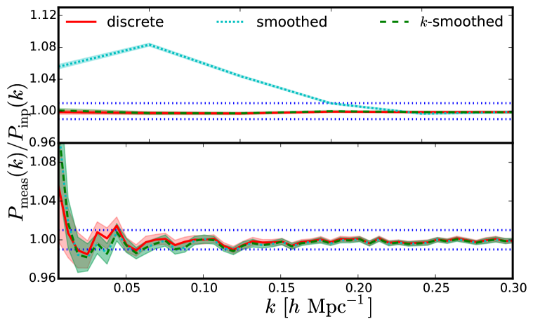
Figure 15: Ratio of the measured power spectrum to the input for three different methods of accounting for the binning effect. (Top) Bin size of $0.05~{}h~{}{\rm Mpc}^{-1}$. (Bottom) Bin size of $0.006~{}h~{}{\rm Mpc}^{-1}$, which is the fundamental frequency in our mock catalog. The three methods are shown in the red solid (discrete), cyan dotted (smoothed), and green dashed ($k$-smoothed) lines. The band denotes the error on the mean measured from 50 realisations. The cyan and green bands overlap in the bottom panel.

Appendix C Mean pairwise line-of-sight velocity in log-normal mock catalog

From equation (4.14), we find that the mean of the pairwise line-of-sight velocity is given by

$$\left[1+\xi_{gg}(r)\right]\left\langle\Delta v_{z}\right\rangle=\left\langle v_{1z}\delta_{g2}\right\rangle-\left\langle v_{2z}\delta_{g1}\right\rangle+\left\langle v_{1z}\delta_{g1}\delta_{g2}\right\rangle-\left\langle v_{2z}\delta_{g2}\delta_{g1}\right\rangle\,,$$ (C.1)

where we use $\left\langle v_{1z}\right\rangle=\left\langle v_{2z}\right\rangle$ and $\left\langle v_{1z}\delta_{g1}\right\rangle=\left\langle v_{2z}\delta_{g2}\right\rangle$ from homogeneity and isotropy. Thus, to compute the mean of the pairwise line-of-sight velocity, we need the contributions from both two- and three-point functions.

The two-point function contribution is given by

$$\left\langle v_{iz}\delta_{gj}\right\rangle=i\mathcal{H}f\int\frac{d^{3}k}{(2\pi)^{3}}\frac{k_{z}}{k^{2}}P_{gm}(k)e^{i\mbox{\boldmath$k$}\cdot\mbox{\boldmath$r$}_{ij}}=i\mathcal{H}f\mu\int\frac{dk}{2\pi^{2}}kP_{gm}(k)j_{1}(kr_{ij})\,,$$ (C.2)

where $\mbox{\boldmath$r$}_{ij}\equiv\mbox{\boldmath$x$}_{i}-\mbox{\boldmath$x$}_{j}$, $\mu\equiv\hat{z}\cdot\hat{r}_{ij}$ and $j_{1}(x)$ is the spherical Bessel function of the first order. Note that this product is anti-symmetric under the exchange of $i$ and $j$, hence $\left\langle v_{1z}\delta_{g2}\right\rangle-\left\langle v_{2z}\delta_{g1}\right\rangle=2\left\langle v_{1z}\delta_{g2}\right\rangle$. Using equations (4.4)–(4.5), equation (C.2) can be evaluated numerically as a function of $r$ and $\mu$. The blue dashed line in figure 16 shows its contribution to the mean pairwise line-of-sight velocity for $\mu=0.995$. We find that as the separation approaches to zero, this contribution drops to zero since $j_{1}(x)\to 0$ for $x\to 0$. The contribution also decreases with increasing separation, which is a generic feature following the trend of the density two-point correlation function.

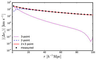
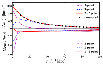
Figure 16: Calculation of the mean pairwise line-of-sight ($\mu=0.995$) velocity in our log-normal mock catalogs, in log scale (left) and linear scale (right, top), along with the residuals (right, bottom). The magenta dotted, blue dashed, and red solid lines show the contributions from three-point function alone, two-point function alone, and two- and three-point functions, respectively. The black points show the measurement from the log-normal mock catalogs and the green dashed line in the bottom right panel shows 1.

For the three-point function contribution, we have

$$\left\langle v_{iz}\delta_{gi}\delta_{gj}\right\rangle=i\mathcal{H}f\int d^{3}x_{p}\frac{d^{3}k}{(2\pi)^{3}}\frac{k_{z}}{k^{2}}e^{i\mbox{\boldmath$k$}\cdot\mbox{\boldmath$r$}_{ij}}\left\langle\delta_{m}(\mbox{\boldmath$x$}_{p})\delta_{g}(\mbox{\boldmath$x$}_{i})\delta_{g}(\mbox{\boldmath$x$}_{j})\right\rangle\,,$$ (C.3)

which is an integral over the three-point function of the (matter and galaxy) density fields. As the velocity field is linearly related to the density field in Fourier space and the three-point function is only calculated easily in configuration space, we need to introduce another vector variable $\mbox{\boldmath$x$}_{p}$ to evaluate this contribution. If the density fields are Gaussian, then this term vanishes and we do not get any contribution. However, for log-normal fields this term is non-zero and is given by [33]

$$\left\langle\delta_{m}(\mbox{\boldmath$x$}_{p})\delta_{g}(\mbox{\boldmath$x$}_{i})\delta_{g}(\mbox{\boldmath$x$}_{j})\right\rangle=\> \xi_{gm}(r_{pi})\xi_{gm}(r_{pj})\xi_{gg}(r_{ij})+$$

$$\xi_{gm}(r_{pi})\xi_{gg}(r_{ij})+\xi_{gm}(r_{pj})\xi_{gg}(r_{ij})+\xi_{gm}(r_{pi})\xi_{gm}(r_{pj})\,,$$ (C.4)

which can be evaluated for our mock catalogs. The magenta dotted line in figure 16 shows this contribution. We find that the contribution decreases with increasing separation, with an upturn at around the BAO scale. The two-point function contribution dominates on most scales except on very small scales.

Combining the contributions from both two- and three-point functions, we find good agreement between the analytic prediction and the measurement in the log-normal mock catalogs, as demonstrated in figure 10.

Appendix D Code Documentation

D.1 Overview

Our mock generator code generates mock galaxy catalogs in redshift space, assuming that the galaxy and matter density fluctuations of the Universe follow a log-normal distribution. Since the code is computationally inexpensive, one can easily generate plentiful realisations with a large volume and a vast number of galaxies. This property is convenient for studying systematics such as the survey window function as well as to evaluate a covariance matrix of the galaxy power spectrum for the current and planned large-scale structure surveys.

D.2 Details

D.2.1 Input file

To run the code, one has to first prepare the configuration file which should contain all the specifications of the model. In this file one needs to specify the input cosmological parameters, volume, output redshift, galaxy bias, number of galaxies, etc. One also needs to specify some key parameters for the execution mode of the code (e.g., the number of realisations, the number of parallel threads to use, the choice of the power spectrum estimator, etc.). The code automatically calculates the input matter power spectrum with the cosmological parameters specified in the configuration file, using the transfer function provided by Eisenstein & Hu [79, 89]. The power spectrum calculated by other codes (e.g., CAMB [90]) can also be used as a tabulated input. The code also calculates the linear growth rate at the output redshift as a function of wave number $k$, taking into account the effect of massive neutrinos [89]. The linear growth rate is used to calculate the velocity field later on.

D.2.2 Generating log-normal density field and mock galaxy catalog

Here we briefly summarize the procedure for generating mock galaxy catalogs using our code (see section 3 for further details).

1. Inverse-Fourier-transform the input power spectrum $P(k)$ to obtain the two-point correlation function $\xi(r)$; calculate the two-point correlation function of the Gaussian field $\xi^{G}(r)$ by equation (3.2); Fourier-transform $\xi^{G}(r)$ to obtain $P^{G}(k)$.

2. Generate a Gaussian random field $G(\mbox{\boldmath$k$})$ for each cell in Fourier space from $P^{G}(k)$, using equation (3.3); Fourier transform $G(\mbox{\boldmath$k$})$ to obtain $G(\mbox{\boldmath$x$})$ and log-transform $G(\mbox{\boldmath$x$})$ to obtain the log-normal density fluctuation $\delta(\mbox{\boldmath$x$})$. The code generates $\delta(\mbox{\boldmath$x$})$ for both biased (i.e., galaxy) and unbiased (i.e., matter) density fields.

3. Generate a velocity field from the matter density fluctuation using the linear continuity equation (3.4).

4. Generate discrete galaxy positions from the galaxy density fluctuation by Poisson sampling the density field in each cell with galaxies being randomly distributed within the cell.

The code outputs the mock galaxy catalog to a binary file. This file contains the 3-D positions and velocity components of each galaxy in units of $~{}h^{-1}~{}{\rm Mpc}$ and km/s respectively.

D.2.3 Estimating the power spectrum multipoles

The next step is to estimate the power spectrum from the simulated galaxy catalog. In our code we use FFT to do this [88]. FFT requires a local number density of galaxies at regular grid points. The code has two options for the density assignment scheme; the Nearest-Grid-Point (NGP) assignment and the Cloud-In-Cell (CIC) assignment. See [80] for the details of the effect of density assignment on the power spectrum estimation with FFT.

What we want to measure is the galaxy power spectrum multipoles $P_{l}(k)$ defined as

$$P(k,\mu)=\sum_{l=0}^{\infty}P_{l}(k)\mathcal{L}_{l}(\mu)\,,$$ (D.1)

where $\mathcal{L}_{l}$ is the $l$-th order Legendre polynomial. The two-dimensional power spectrum $P(k,\mu)$ is estimated from the simulated galaxy catalog as

$$P(k,\mu)=W^{-2}_{\rm mesh}(\bm{k})\left[\dfrac{1}{N_{k}}\sum^{N_{k}}_{i=1}|\delta_{g}(\bm{k}_{i})|^{2}-P_{\text{shot}}\right]\,,$$ (D.2)

where $\delta_{g}(\bm{k})$ is the Fourier transformed local galaxy number density contrast, $N_{k}$ is the number of Fourier modes within the given $k$ bin, $P_{\text{shot}}$ is the power spectrum for a uniform random distribution of particles (shot noise), and $\mu$ is the cosine of the angle between $k$ and the line-of-sight vector. Here we assume that the line-of-sight vector is the same for all galaxies (i.e., global plane-parallel approximation). The mesh window function $W_{\rm mesh}(k)$ is the Fourier transform of the density assignment scheme, that is $W_{\rm mesh}(k)=\left[\sin(kH/2)/(kH/2)\right]^{p}$, where $H$ is the mesh size, and $p=1$ and $2$ for NGP and CIC, respectively. The shot noise contribution for NGP and CIC is calculated analytically [77]. For NGP, if we use the same mesh size as the log-normal galaxy realisation, we do not need to correct for the density assignment. This is because the log-normal realisation code also uses FFT and density fields are generated at regular grid points.

To estimate the true power spectrum multipoles $P_{l}(k)$, we first compute a brute-force estimate $\hat{P}_{m}(k)$ as

$$\hat{P}_{m}(k)=\sum_{\mu}P(k,\mu)\mathcal{L}_{m}(\mu)\,.$$ (D.3)

Using equation (D.1), $\hat{P}_{m}(k)$ can be rewritten as

$$\hat{P}_{m}(k)=\sum_{\mu}\sum_{l=0}^{\infty}P_{l}(k)\mathcal{L}_{l}(\mu)\mathcal{L}_{m}(\mu)=\sum_{l=0}^{\infty}P_{l}(k)\mathcal{M}_{lm},$$ (D.4)

where $\mathcal{M}_{lm}$ is the $\mu$-leakage matrix defined as

$$\mathcal{M}_{lm}=\sum_{\mu}\mathcal{L}_{l}(\mu)\mathcal{L}_{m}(\mu).$$ (D.5)

Then the true power spectrum multipoles $P_{l}(k)$ can be calculated as

$$P_{l}(k)=\sum_{m=0}^{\infty}\hat{P}_{m}(k)\mathcal{M}^{-1}_{lm},$$ (D.6)

where $\mathcal{M}^{-1}_{lm}$ is the inverse matrix of $\mathcal{M}_{lm}$. Note that $\mathcal{M}_{lm}$ is computed for each $k$ separately. While the sum over $m$ goes to $\infty$, we only sum up to a certain maximum value, specified as an input in the configuration file.

Depending on the geometry of the volume, the matrix inversion of $\mathcal{M}_{lm}$ sometimes becomes unstable particularly at low $k$ where the number of $\mu$ modes for a fixed $k$ is limited. To avoid this problem we include another option for the power spectrum estimation, that is, the “cubic box mode”. In this mode the mocked volume (it is rectangular cuboid in general) is embedded in a cube which is large enough to contain the whole mocked box, setting $\delta_{g}(\mbox{\boldmath$x$})=0$ outside of the mock catalog box. This procedure enables us to have a sufficient number of $\mu$ modes even at a small $k$. However, in the cubic box mode, $P_{l}(k)$ is convolved with the survey window function $W(\bm{r})$: namely, $W(\bm{r})=1$ if $\bm{r}$ is within the mock catalog box and $W(\bm{r})=0$ otherwise. We need to correct this survey window effect when comparing with the theoretical predictions of the power spectrum multipoles. For the treatment of the survey window function in redshift space, we refer the reader to, e.g. [91].

D.2.4 Test the code

To check the results, run some number of realisations, compute real-space monopole power spectra, average them, and compare the average with the input matter power spectrum times the bias squared. The average should precisely reproduce the input power spectrum on large scales, although it would deviate from the input on small scales due to the resolution effect of Fourier meshes. See figure 2.

References

- [1] W. Percival, The Invisible Universe: Dark Matter and Dark Energy. Springer Berlin Heidelberg, Berlin, Heidelberg, 2007, 10.1007/978-3-540-71013-46.
- [2] BOSS collaboration, S. Alam et al., The clustering of galaxies in the completed SDSS-III Baryon Oscillation Spectroscopic Survey: cosmological analysis of the DR12 galaxy sample, Submitted to: Mon. Not. Roy. Astron. Soc. (2016) , [1607.03155].
- [3] WMAP collaboration, C. L. Bennett et al., Nine-Year Wilkinson Microwave Anisotropy Probe (WMAP) Observations: Final Maps and Results, Astrophys. J. Suppl. 208 (2013) 20, [1212.5225].
- [4] Planck collaboration, R. Adam et al., Planck 2015 results. I. Overview of products and scientific results, Astron. Astrophys. 594 (2016) A1, [1502.01582].
- [5] SNLS collaboration, A. Conley et al., Supernova Constraints and Systematic Uncertainties from the First 3 Years of the Supernova Legacy Survey, Astrophys. J. Suppl. 192 (2011) 1, [1104.1443].
- [6] N. Suzuki et al., The Hubble Space Telescope Cluster Supernova Survey: V. Improving the Dark Energy Constraints Above and Building an Early-Type-Hosted Supernova Sample, Astrophys. J. 746 (2012) 85, [1105.3470].
- [7] F. Bernardeau, S. Colombi, E. Gaztanaga and R. Scoccimarro, Large scale structure of the universe and cosmological perturbation theory, Phys. Rept. 367 (2002) 1–248, [astro-ph/0112551].
- [8] V. Desjacques, D. Jeong and F. Schmidt, Large-Scale Galaxy Bias, 1611.09787.
- [9] I. Mohammed, U. Seljak and Z. Vlah, Perturbative approach to covariance matrix of the matter power spectrum, Mon. Not. Roy. Astron. Soc. 466 (2017) 780–797, [1607.00043].
- [10] A. Barreira and F. Schmidt, Responses in Large-Scale Structure, 1703.09212.
- [11] D. Baumann, A. Nicolis, L. Senatore and M. Zaldarriaga, Cosmological non-linearities as an effective fluid, JCAP 7 (July, 2012) 051, [1004.2488].
- [12] J. J. M. Carrasco, M. P. Hertzberg and L. Senatore, The effective field theory of cosmological large scale structures, JHEP 9 (Sept., 2012) 82, [1206.2926].
- [13] C.-T. Chiang et al., Galaxy redshift surveys with sparse sampling, JCAP 1312 (2013) 030, [1306.4157].
- [14] H. Guo et al., Redshift-space clustering of SDSS galaxies – luminosity dependence, halo occupation distribution, and velocity bias, Mon. Not. Roy. Astron. Soc. 453 (2015) 4368–4383, [1505.07861].
- [15] S. Saito et al., Connecting massive galaxies to dark matter haloes in BOSS – I. Is galaxy colour a stochastic process in high-mass haloes?, Mon. Not. Roy. Astron. Soc. 460 (2016) 1457–1475, [1509.00482].
- [16] S. Dodelson and M. D. Schneider, The Effect of Covariance Estimator Error on Cosmological Parameter Constraints, Phys. Rev. D88 (2013) 063537, [1304.2593].
- [17] J. Hartlap, P. Simon and P. Schneider, Why your model parameter confidences might be too optimistic: Unbiased estimation of the inverse covariance matrix, Astron. Astrophys. (2006) , [astro-ph/0608064].
- [18] E. Sellentin and A. F. Heavens, Quantifying lost information due to covariance matrix estimation in parameter inference, Mon. Not. Roy. Astron. Soc. 464 (2017) 4658–4665, [1609.00504].
- [19] Y. B. Zel’dovich, Gravitational instability: An approximate theory for large density perturbations., Astron. Astrophys. 5 (Mar., 1970) 84–89.
- [20] F. Moutarde, J.-M. Alimi, F. R. Bouchet, R. Pellat and A. Ramani, Precollapse scale invariance in gravitational instability, Astrophys. J. 382 (Dec., 1991) 377–381.
- [21] T. Buchert and J. Ehlers, Lagrangian theory of gravitational instability of Friedman-Lemaitre cosmologies – second-order approach: an improved model for non-linear clustering, Mon. Not. Roy. Astron. Soc. 264 (Sept., 1993) .
- [22] P. Catelan, Lagrangian dynamics in non-flat universes and non-linear gravitational evolution, Mon. Not. Roy. Astron. Soc. 276 (Sept., 1995) 115–124, [astro-ph/9406016].
- [23] P. Coles, A. L. Melott and S. F. Shandarin, Testing approximations for non-linear gravitational clustering, Mon. Not. Roy. Astron. Soc. 260 (Feb., 1993) 765–776.
- [24] A. L. Melott, T. Buchert and A. G. Weib, Testing higher-order Lagrangian perturbation theory against numerical simulations. 2: Hierarchical models, Astron. Astrophys. 294 (Feb., 1995) 345–365, [astro-ph/9404018].
- [25] F.-S. Kitaura and S. Heß, Cosmological structure formation with augmented Lagrangian perturbation theory, Mon. Not. Roy. Astron. Soc. 435 (Aug., 2013) L78–L82, [1212.3514].
- [26] S. Tassev, M. Zaldarriaga and D. J. Eisenstein, Solving large scale structure in ten easy steps with COLA, ”JCAP” 6 (June, 2013) 036, [1301.0322].
- [27] M. C. Neyrinck, Truthing the stretch: non-perturbative cosmological realizations with multiscale spherical collapse, Mon. Not. Roy. Astron. Soc. 455 (Jan., 2016) L11–L15, [1503.07534].
- [28] J. Koda, C. Blake, F. Beutler, E. Kazin and F. Marin, Fast and accurate mock catalogue generation for low-mass galaxies, Mon. Not. Roy. Astron. Soc. 459 (June, 2016) 2118–2129, [1507.05329].
- [29] P. Monaco, Approximate Methods for the Generation of Dark Matter Halo Catalogs in the Age of Precision Cosmology, Galaxies 4 (Oct., 2016) 53, [1605.07752].
- [30] A. L. Melott, Comparison of dynamical approximation schemes for nonlinear gravitaional clustering, Astrophys. J. Lett. 426 (May, 1994) , [astro-ph/9402057].
- [31] C.-H. Chuang et al., nIFTy Cosmology: Galaxy/halo mock catalogue comparison project on clustering statistics, Mon. Not. Roy. Astron. Soc. 452 (2015) 686–700, [1412.7729].
- [32] E. Munari, P. Monaco, J. Koda, F.-S. Kitaura, E. Sefusatti and S. Borgani, Testing approximate predictions of displacements of cosmological dark matter halos, ArXiv e-prints (Apr., 2017) , [1704.00920].
- [33] P. Coles and B. Jones, A Lognormal model for the cosmological mass distribution, Mon. Not. Roy. Astron. Soc. 248 (1991) 1–13.
- [34] S. Colombi, A ’skewed’ lognormal approximation to the probablility distribution function of the large-scale density field, Astrophys. J. 435 (Nov., 1994) 536–539, [astro-ph/9402071].
- [35] L. Kofman, E. Bertschinger, J. M. Gelb, A. Nusser and A. Dekel, Evolution of one-point distributions from Gaussian initial fluctuations, Astrophys. J. 420 (Jan., 1994) 44–57, [astro-ph/9311028].
- [36] F. Bernardeau and L. Kofman, Properties of the cosmological density distribution function, Astrophys. J. 443 (Apr., 1995) 479–498, [astro-ph/9403028].
- [37] C. Uhlemann, S. Codis, C. Pichon, F. Bernardeau and P. Reimberg, Back in the saddle: large-deviation statistics of the cosmic log-density field, Mon. Not. Roy. Astron. Soc. 460 (Aug., 2016) 1529–1541, [1512.05793].
- [38] J. Shin, J. Kim, C. Pichon, D. Jeong and C. Park, New fitting formula for cosmic non-linear density distribution, ArXiv e-prints (May, 2017) , [1705.06863].
- [39] DES collaboration, L. Clerkin et al., Testing the lognormality of the galaxy and weak lensing convergence distributions from Dark Energy Survey maps, Submitted to: Mon. Not. Roy. Astron. Soc. (2016) , [1605.02036].
- [40] E. Hubble, The Distribution of Extra-Galactic Nebulae, Astrophys. J. 79 (Jan., 1934) 8.
- [41] 2dFGRS collaboration, V. Wild et al., The 2dF Galaxy Redshift Survey: Stochastic relative biasing between galaxy populations, Mon. Not. Roy. Astron. Soc. 356 (2005) 247, [astro-ph/0404275].
- [42] I. Kayo, A. Taruya and Y. Suto, Probability distribution function of cosmological density fluctuations from Gaussian initial condition: comparison of one- and two-point log-normal model predictions with n-body simulations, Astrophys. J. 561 (2001) 22–34, [astro-ph/0105218].
- [43] R. Scoccimarro, Redshift-space distortions, pairwise velocities and nonlinearities, Phys. Rev. D70 (2004) 083007, [astro-ph/0407214].
- [44] D. W. Pearson, L. Samushia and P. Gagrani, Optimal weights for measuring redshift space distortions in multitracer galaxy catalogues, Mon. Not. Roy. Astron. Soc. 463 (2016) 2708–2715, [1606.03435].
- [45] H. S. Xavier, F. B. Abdalla and B. Joachimi, Improving lognormal models for cosmological fields, Mon. Not. Roy. Astron. Soc. 459 (2016) 3693–3710, [1602.08503].
- [46] D. Alonso, P. G. Ferreira and M. G. Santos, Fast simulations for intensity mapping experiments, Mon. Not. Roy. Astron. Soc. 444 (2014) 3183, [1405.1751].
- [47] D. Jeong, F. Schmidt and C. M. Hirata, Large-scale clustering of galaxies in general relativity, Phys. Rev. D85 (Jan., 2012) 023504, [1107.5427].
- [48] N. Kaiser, Clustering in real space and in redshift space, Mon. Not. Roy. Astron. Soc. 227 (1987) 1–27.
- [49] A. J. S. Hamilton, Measuring Omega and the real correlation function from the redshift correlation function, Astrophys. J. Lett. 385 (Jan., 1992) L5–L8.
- [50] A. J. S. Hamilton, Linear Redshift Distortions: a Review, in The Evolving Universe (D. Hamilton, ed.), vol. 231 of Astrophysics and Space Science Library, p. 185, 1998, astro-ph/9708102, DOI.
- [51] J. C. Jackson, Fingers of God: A critique of Rees’ theory of primoridal gravitational radiation, Mon. Not. Roy. Astron. Soc. 156 (1972) 1P–5P, [0810.3908].
- [52] A. F. Heavens, S. Matarrese and L. Verde, The Nonlinear redshift-space power spectrum of galaxies, Mon. Not. Roy. Astron. Soc. 301 (1998) 797–808, [astro-ph/9808016].
- [53] T. Matsubara, Resumming Cosmological Perturbations via the Lagrangian Picture: One-loop Results in Real Space and in Redshift Space, Phys. Rev. D77 (2008) 063530, [0711.2521].
- [54] T. Matsubara, Nonlinear perturbation theory with halo bias and redshift-space distortions via the Lagrangian picture, Phys. Rev. D78 (2008) 083519, [0807.1733].
- [55] T. Matsubara, Nonlinear Perturbation Theory Integrated with Nonlocal Bias, Redshift-space Distortions, and Primordial Non-Gaussianity, Phys. Rev. D83 (2011) 083518, [1102.4619].
- [56] T. Matsubara, Integrated Perturbation Theory and One-loop Power Spectra of Biased Tracers, Phys. Rev. D90 (2014) 043537, [1304.4226].
- [57] N. S. Sugiyama, Using Lagrangian perturbation theory for precision cosmology, Astrophys. J. 788 (2014) 63, [1311.0725].
- [58] M. Lewandowski, L. Senatore, F. Prada, C. Zhao and C.-H. Chuang, On the EFT of Large Scale Structures in Redshift Space, 1512.06831.
- [59] A. Perko, L. Senatore, E. Jennings and R. H. Wechsler, Biased Tracers in Redshift Space in the EFT of Large-Scale Structure, 1610.09321.
- [60] U. Seljak and P. McDonald, Distribution function approach to redshift space distortions, JCAP 1111 (2011) 039, [1109.1888].
- [61] T. Okumura, U. Seljak, P. McDonald and V. Desjacques, Distribution function approach to redshift space distortions. Part II: N-body simulations, JCAP 1202 (2012) 010, [1109.1609].
- [62] T. Okumura, U. Seljak and V. Desjacques, Distribution function approach to redshift space distortions, Part III: halos and galaxies, JCAP 1211 (2012) 014, [1206.4070].
- [63] Z. Vlah, U. Seljak, P. McDonald, T. Okumura and T. Baldauf, Distribution function approach to redshift space distortions. Part IV: perturbation theory applied to dark matter, JCAP 1211 (2012) 009, [1207.0839].
- [64] Z. Vlah, U. Seljak, T. Okumura and V. Desjacques, Distribution function approach to redshift space distortions. Part V: perturbation theory applied to dark matter halos, JCAP 1310 (2013) 053, [1308.6294].
- [65] T. Okumura, N. Hand, U. Seljak, Z. Vlah and V. Desjacques, Galaxy power spectrum in redshift space: combining perturbation theory with the halo model, Phys. Rev. D92 (2015) 103516, [1506.05814].
- [66] A. Taruya, T. Nishimichi and S. Saito, Baryon Acoustic Oscillations in 2D: Modeling Redshift-space Power Spectrum from Perturbation Theory, Phys. Rev. D82 (2010) 063522, [1006.0699].
- [67] L. Wang, B. Reid and M. White, An analytic model for redshift-space distortions, Mon. Not. Roy. Astron. Soc. 437 (2014) 588–599, [1306.1804].
- [68] P. J. E. Peebles, The large-scale structure of the universe. 1980.
- [69] M. Davis and P. J. E. Peebles, A Survey of galaxy redshifts. 5. The Two point position and velocity correlations, Astrophys. J. 267 (1982) 465–482.
- [70] K. B. Fisher, On the validity of the streaming model for the redshift space correlation function in the linear regime, Astrophys. J. 448 (1995) 494–499, [astro-ph/9412081].
- [71] C. Uhlemann, M. Kopp and T. Haugg, Edgeworth streaming model for redshift space distortions, Phys. Rev. D92 (2015) 063004, [1503.08837].
- [72] D. Jeong, L. Dai, M. Kamionkowski and A. S. Szalay, The redshift-space galaxy two-point correlation function and baryon acoustic oscillations, Mon. Not. Roy. Astron. Soc. 449 (May, 2015) 3312–3322, [1408.4648].
- [73] R. de Putter, C. Wagner, O. Mena, L. Verde and W. Percival, Thinking Outside the Box: Effects of Modes Larger than the Survey on Matter Power Spectrum Covariance, JCAP 1204 (2012) 019, [1111.6596].
- [74] D. Bianchi, W. Percival and J. Bel, Improving the modelling of redshift-space distortions - II. A pairwise velocity model covering large and small scales, 1602.02780.
- [75] L. Wang, B. Reid and M. White, An analytic model for redshift-space distortions, Mon. Not. Roy. Astron. Soc. 437 (2014) 588–599, [1306.1804].
- [76] B. A. Reid and M. White, Towards an accurate model of the redshift space clustering of halos in the quasilinear regime, Mon. Not. Roy. Astron. Soc. 417 (2011) 1913–1927, [1105.4165].
- [77] D. Jeong, Cosmology with high (z1) redshift galaxy surveys, Ph.D. thesis, The University of Texas at Austin, 2010.
- [78] “Fastest Fourier Transform in the West.”
- [79] D. J. Eisenstein and W. Hu, Baryonic features in the matter transfer function, Astrophys. J. 496 (1998) 605, [astro-ph/9709112].
- [80] Y. P. Jing, Correcting for the alias effect when measuring the power spectrum using FFT, Astrophys. J. 620 (2005) 559–563, [astro-ph/0409240].
- [81] S. D. Landy and A. S. Szalay, Bias and variance of angular correlation functions, Astrophys. J. 412 (1993) 64.
- [82] G. J. Hill et al., The Hobby-Eberly Telescope Dark Energy Experiment (HETDEX): Description and Early Pilot Survey Results, ASP Conf. Ser. 399 (2008) 115–118, [0806.0183].
- [83] N. Tamura et al., Prime Focus Spectrograph (PFS) for the Subaru Telescope: Overview, recent progress, and future perspectives, Proc. SPIE Int. Soc. Opt. Eng. 9908 (2016) 99081M, [1608.01075].
- [84] D. Spergel et al., Wide-Field InfrarRed Survey Telescope-Astrophysics Focused Telescope Assets WFIRST-AFTA 2015 Report, 1503.03757.
- [85] DESI collaboration, M. Levi et al., The DESI Experiment, a whitepaper for Snowmass 2013, 1308.0847.
- [86] P. A. Abell, J. Allison, S. F. Anderson, J. R. Andrew, J. R. P. Angel, L. Armus et al., Lsst science book, version 2.0, 0912.0201.
- [87] EUCLID collaboration, R. Laureijs et al., Euclid Definition Study Report, 1110.3193.
- [88] H. A. Feldman, N. Kaiser and J. A. Peacock, Power spectrum analysis of three-dimensional redshift surveys, Astrophys. J. 426 (1994) 23–37, [astro-ph/9304022].
- [89] D. J. Eisenstein and W. Hu, Power spectra for cold dark matter and its variants, Astrophys. J. 511 (1997) 5, [astro-ph/9710252].
- [90] A. Lewis, A. Challinor and A. Lasenby, Efficient computation of CMB anisotropies in closed FRW models, Astrophys. J. 538 (2000) 473–476, [astro-ph/9911177].
- [91] BOSS collaboration, F. Beutler et al., The clustering of galaxies in the SDSS-III Baryon Oscillation Spectroscopic Survey: Testing gravity with redshift-space distortions using the power spectrum multipoles, Mon. Not. Roy. Astron. Soc. 443 (2014) 1065–1089, [1312.4611].