Multiple-Relaxation-Time Lattice Boltzmann scheme for Fractional Advection-Diffusion Equation

Abstract

Partial differential equations (p.d.e) equipped with spatial derivatives of fractional order capture anomalous transport behaviors observed in diverse fields of Science. A number of numerical methods approximate their solutions in dimension one. Focusing our effort on such p.d.e. in higher dimension with Dirichlet boundary conditions, we present an approximation based on Lattice Boltzmann Method with Bhatnagar-Gross-Krook (BGK) or Multiple-Relaxation-Time (MRT) collision operators. First, an equilibrium distribution function is defined for simulating space-fractional diffusion equations in dimensions 2 and 3. Then, we check the accuracy of the solutions by comparing with i) random walks derived from stable Lévy motion, and ii) exact solutions. Because of its additional freedom degrees, the MRT collision operator provides accurate approximations to space-fractional advection-diffusion equations, even in the cases which the BGK fails to represent because of anisotropic diffusion tensor or of flow rate destabilizing the BGK LBM scheme.

1 Introduction

Among diverse non-Fickian transport behaviors observed in all fields of Science, heavy tailed spatial concentration profiles recorded on chemical species, living cells or organisms, suggest displacements more rapid than the classical Advection Diffusion Equation (ADE) predicts [1, 2, 3, 4, 5]. Such super-dispersive phenomena include plumes that lack finite second moment, or whose mean and peak do not coincide (see [6]). Possible explanations may be large scale heterogeneity or multiple coupling between many simple sub-systems which separately would not exhibit such abnormalities. Similar strange behaviors are observed often enough to suggest exploring alternative models as fractional partial differential equations. It turns out that [7, 6, 8, 9, 10] many tracer tests in rivers and underground porous media are accurately represented by the more general conservation equation

$$\frac{\partial C}{\partial t}(\mathbf{x},\,t)+\boldsymbol{\nabla}\cdot(\mathbf{u}C)(\mathbf{x},\,t)=\boldsymbol{\nabla}\cdot\overline{\overline{\mathbf{D}}}(\mathbf{x})\boldsymbol{\mathcal{F}}^{\boldsymbol{\alpha}\boldsymbol{p}\boldsymbol{g}}(C)+S_{c}(\mathbf{x},\,t).$$ (1)

It models mass spreading for passive solute at concentration $C$ in incompressible fluid flowing at average flow rate $\mathbf{u}=\sum_{\mu=1}^{d}u_{\mu}\mathbf{b}_{\mu}$ super-imposed to small scale velocity field whose complexity causes non-Fickian dispersive flux $-\overline{\overline{\mathbf{D}}}\boldsymbol{\mathcal{F}}^{\boldsymbol{\alpha}\boldsymbol{p}\boldsymbol{g}}(C)$. The space variable $\mathbf{x}$ belongs to some domain $\Omega$ of $\mathbb{R}^{d}$, and is described in the orthonormal basis $\{\mathbf{b}_{\mu};\,\mbox{for }\mu=1,\,...,\,d\}$ of $\mathbb{R}^{d}$ by its coordinates noted $x_{\mu}$: greek subscripts refer to spatial coordinates. Moreover $S_{c}$ is a source rate. The coordinates of vector $\boldsymbol{\mathcal{F}}^{\boldsymbol{\alpha}\boldsymbol{p}\boldsymbol{g}}(C)$ are composed of partial derivatives of $C$ with respect to (w.r.t.) the $x_{\mu}$ which reflect the variations of $C$ when all the other coordinates of $\mathbf{x}$ are fixed. These derivatives are of order one in the classical ADE, but in Eq. (1) they may have fractional order $\alpha_{\mu}-1$ specified by the entries of vector $\boldsymbol{\alpha}=(\alpha_{1},\,...,\,\alpha_{d})^{T}$ which belong to $]1,\,2]$. Yet, in general fractional derivatives are not completely determined by their order. This is why vector $\boldsymbol{\mathcal{F}}^{\boldsymbol{\alpha}\boldsymbol{p}\boldsymbol{g}}(C)$ also depends on parameters $p_{\mu}\in[0,\,1]$ which we gather in a vector $\boldsymbol{p}=(p_{1},\,...\,p_{d})^{T}$. The coordinates $g_{\mu}\in\mathbb{R}_{+}$ of vector $\boldsymbol{g}=(g_{1},\,...\,g_{d})^{T}$ are just positive auxiliary factors, and $\overline{\overline{\mathbf{D}}}$ is a regular diffusivity tensor.

Actually, fractional derivatives w.r.t. $x_{\mu}$ can be viewed as regular derivatives w.r.t. this variable compounded with fractional integrals of the form $I_{x_{\mu}\pm}^{\gamma}$, often thought of as integro-differential operators of negative order $-\gamma$. The fractional integrals are convolutions whose kernel is a Dirac mass at point $0$ if $\gamma=0$, or $(x_{\mu})_{\pm}^{\gamma-1}/\Gamma(\gamma)$ if $\gamma>0$: subscript $\pm$ designates positive or negative part and $\Gamma$ is the Euler Gamma function defined by $\Gamma(x)=\int_{0}^{\infty}t^{x-1}e^{-t}dt$ [11]. With these notations, the vector $\boldsymbol{\mathcal{F}}^{\boldsymbol{\alpha}\boldsymbol{p}\boldsymbol{g}}(C)$ is defined by its components $\mathcal{F}_{\mu}^{\alpha_{\mu}p_{\mu}g_{\mu}}(C)$ in $\{\mathbf{b}_{\mu}\}$ basis

$$\boldsymbol{\mathcal{F}}^{\boldsymbol{\alpha}\boldsymbol{p}\boldsymbol{g}}(C)=\sum_{\mu=1}^{d}\mathcal{F}_{\mu}^{\alpha_{\mu}p_{\mu}g_{\mu}}(C)\mathbf{b}_{\mu},\quad\mathcal{F}_{\mu}^{\alpha_{\mu}p_{\mu}g_{\mu}}(C)=\frac{\partial}{\partial x_{\mu}}\left[p_{\mu}I_{x_{\mu}+}^{2-\alpha_{\mu}}(g_{\mu}C)+(1-p_{\mu})I_{x_{\mu}-}^{2-\alpha_{\mu}}(g_{\mu}C)\right],$$ (2)

in which $p_{\mu}$ and $1-p_{\mu}$ weight the two integrals $I_{x_{\mu}\pm}^{2-\alpha_{\mu}}$. Hence, $\alpha_{\mu}$ sums up all integro-differential orders in the contribution of $\mathcal{F}_{\mu}^{\alpha_{\mu}p_{\mu}g_{\mu}}(C)\mathbf{b}_{\mu}$ to $\boldsymbol{\nabla}\cdot\overline{\overline{\mathbf{D}}}(\mathbf{x})\boldsymbol{\mathcal{F}}^{\boldsymbol{\alpha}\boldsymbol{p}\boldsymbol{g}}(C)$, which writes $\sum_{\nu=1}^{d}\partial(D_{\nu\mu}\mathcal{F}_{\mu}^{\alpha_{\mu}p_{\mu}g_{\mu}}(C))/\partial x_{\nu}$. Since $I_{x_{\mu}+}^{0}$ and $I_{x_{\mu}-}^{0}$ coincide with operator Identity ($\mathrm{Id}$), we immediately see that Eq. (1) is the classical ADE for all values of $\boldsymbol{p}$ in the limit case $\boldsymbol{\alpha}=\boldsymbol{2}=(2,\,...,\,2)$. Transport phenomena deviating from this classical paradigm and reported in [1, 2, 3, 4, 5, 7, 6, 8, 9, 10] are better accounted by $\boldsymbol{\alpha}\neq\boldsymbol{2}$. For $\gamma>0$ the convolution that defines $I_{x_{\mu}+}^{\gamma}C(\mathbf{x},\,t)$ results from integration over interval $\omega_{+}(\mathbf{x},\,\mu)=\{\mathbf{y}\in\Omega/y_{\nu}=x_{\nu}\,\,\mbox{for}\,\,\nu\neq\mu,\,y_{\mu}<x_{\mu}\}$ ending at point $\mathbf{x}$ and parallel to $\mathbf{b}_{\mu}$. In other words, the elements of this interval have exactly the same coordinates as $\mathbf{x}$ except for the coordinate of rank $\mu$ along which the integration is carried out. The other integral $I_{x_{\mu}-}^{\gamma}C$ corresponds to the opposite interval $\omega_{-}(\mathbf{x},\,\mu)=\{\mathbf{y}\in\Omega/y_{\nu}=x_{\nu}\,\,\mbox{for}\,\,\nu\neq\mu,\,y_{\mu}>x_{\mu}\}$, and the complete definition of $I_{x_{\mu}\pm}^{\gamma}$ is

$$(I_{x_{\mu}+}^{\gamma}C)(\mathbf{x})=\frac{1}{\Gamma(\gamma)}\int_{-\infty}^{x_{\mu}}\frac{1_{\omega_{+}(\mathbf{x},\,\mu)}(\mathbf{y})C(\mathbf{y})}{(x_{\mu}-y_{\mu})^{1-\gamma}}dy_{\mu},\qquad\mbox{and}\qquad(I_{x_{\mu}-}^{\gamma}C)(\mathbf{x})=\frac{1}{\Gamma(\gamma)}\int_{x_{\mu}}^{+\infty}\frac{1_{\omega_{-}(\mathbf{x},\,\mu)}(\mathbf{y})C(\mathbf{y})}{(y_{\mu}-x_{\mu})^{1-\gamma}}dy_{\mu}.$$ (3)

In Eq. (3), $1_{E}$ represents the set function of any subset $E$ of $\Omega$, i.e. $1_{E}(\mathbf{x})=1$ for $\mathbf{x}\in E$ and $1_{E}(\mathbf{x})=0$ for $\mathbf{x}\notin E$. Here we more especially consider the domain $\Omega=\Pi_{\mu=1}^{d}]\ell_{\mu},\,L_{\mu}[$, and the two above integrals correspond to intervals $]\ell_{\mu},\,x_{\mu}[$ and $]x_{\mu},\,L_{\mu}[$. For instance, if we assume $d=3$ and $\mu=1$, Eqs (3) write

$$(I_{x_{1}+}^{\gamma}C)(\mathbf{x})=\frac{1}{\Gamma(\gamma)}\int_{\ell_{1}}^{x_{1}}\frac{C(y_{1},\,x_{2},\,x_{3})}{(x_{1}-y_{1})^{1-\gamma}}dy_{1},\qquad\mbox{and}\qquad(I_{x_{1}-}^{\gamma}C)(\mathbf{x})=\frac{1}{\Gamma(\gamma)}\int_{x_{1}}^{L_{1}}\frac{C(y_{1},\,x_{2},\,x_{3})}{(y_{1}-x_{1})^{1-\gamma}}dy_{1}.$$ (4)

The objective of this paper is to propose a LBM scheme applicable to tensor $\overline{\overline{\mathbf{D}}}$ and vector $\boldsymbol{g}$ allowed to depend on $\mathbf{x}$ because this includes a variety of configurations considered by [12, 13] for $\boldsymbol{\alpha}\neq\boldsymbol{2}$ and by [14, 15] in the case of the ADE. Parameters $\boldsymbol{\alpha}$ and $\boldsymbol{p}$ are nevertheless assumed constant in time and space. The definition (2) of $\boldsymbol{\mathcal{F}}^{\boldsymbol{\alpha}\boldsymbol{p}\boldsymbol{g}}(C)$ takes the same form when $\overline{\overline{\mathbf{D}}}$ and $\boldsymbol{g}$ depend on $\mathbf{x}$ or not. Moreover its structure is especially well adapted to the design of LBM schemes approximating Eq. (1), and very comfortable for coding. This is why we prefer the formulation Eq. (2) to equivalent expressions of $\boldsymbol{\mathcal{F}}^{\boldsymbol{\alpha}\boldsymbol{p}\boldsymbol{g}}(C)$ exhibiting fractional derivatives of Riemann-Liouville type [11] defined by

$$\frac{\partial^{\alpha^{\prime}}C}{\partial_{\pm}x_{\mu}^{\alpha^{\prime}}}(\mathbf{x})=\pm\frac{\partial}{\partial x_{\mu}}(I_{x_{\mu}\pm}^{1-\alpha^{\prime}}C)(\mathbf{x})\quad\mbox{for}\quad\alpha^{\prime}\in]0,\,1[,\qquad\frac{\partial^{\alpha^{\prime}}C}{\partial_{\pm}x_{\mu}^{\alpha^{\prime}}}(\mathbf{x})=\frac{\partial^{2}}{\partial x_{\mu}^{2}}(I_{x_{\mu}\pm}^{2-\alpha^{\prime}}C)(\mathbf{x})\quad\mbox{for}\quad\alpha^{\prime}\in]1,\,2[.$$ (5)

For example, Eq. (1) writes

$$\frac{\partial C}{\partial t}(\mathbf{x},\,t)+\boldsymbol{\nabla}\cdot(\mathbf{u}C)(\mathbf{x},\,t)=\sum_{\mu=1}^{d}D_{\mu\mu}\left[p_{\mu}\frac{\partial^{\alpha_{\mu}}g_{\mu}C}{\partial_{+}x_{\mu}^{\alpha_{\mu}}}+(1-p_{\mu})\frac{\partial^{\alpha_{\mu}}g_{\mu}C}{\partial_{-}x_{\mu}^{\alpha_{\mu}}}\right]+S_{c}(\mathbf{x},\,t)$$ (6)

when tensor $\overline{\overline{\mathbf{D}}}$ is diagonal and spatially homogeneous, but this formulation becomes heavier than Eqs (1)-(2) in more general cases. Moreover, we assume non-dimensional variables and parameters in Eqs (1) and (2).

Eq. (1) is more than just a model for solute transport. It rules the evolution of the probability density function (p.d.f) of a wide set of stochastic processes [12] called stable. Stable processes include finite or infinite variance and are more general than Brownian motion which corresponds to the particular case $\boldsymbol{\alpha}=\boldsymbol{2}$. They are related to stable probability laws which deserve the attention of physicists because they are attractors (for limits of sums of independent identically distributed random variables) [16]. Moreover, experimental techniques (not restricted to concentrations of particles) document individual trajectories of animals [3] or characteristic functions of molecular displacements [17] measured by Pulse Field Gradient Nuclear Magnetic Resonance. They reveal stable motion in different fields of Science such as biology and fluid dynamics [18]. More specifically, the latter reference points stable motion at small scale in water flowing through packed grains exhibiting sharp edges, a material that looks homogeneous: heterogeneity of flow inside pores might explain anomalous transport in this case. Though multidimensional stable motions are more diverse [13, 19] we just mention here those which have independent stable projections on the $\mathbf{b}_{\mu}$: their density satisfies Eq. (1) equipped with spatially homogeneous $\overline{\overline{\mathbf{D}}}$ tensor diagonal in this basis. Moreover, the Riemann-Liouville derivatives included in the definition (2) of $\boldsymbol{\mathcal{F}}^{\boldsymbol{\alpha}\boldsymbol{p}\boldsymbol{g}}$ actually represent the particle fluxes generated by such stable process [20]. This designates these derivatives as privileged elements of this vector beside variants discussed in [21] and in Subsection 3.5 of the present paper.

The many possible applications of Eq. (1) motivate simulation efforts. Finite difference/volume/element schemes are available [22, 23, 24], and particle tracking is a powerful method [12] based on the tight relationship to stable processes [13]. Yet, the computing time requested by these methods (even the latter) causes that increasing the space dimension $d$ enhances the attractivity of the LBM. The latter method simulates evolution equations by considering an ensemble of fictitious particles whose individual velocities belong to a discrete set, namely the elementary grid of a lattice. More specifically, the densities of populations experiencing each of these velocities evolve according to Boltzmann Equation modeling displacements interspersed with instantaneous collisions. Adapting the collision rules causes that the total density satisfies the p.d.e which we want to simulate. This method was applied to equations of the form of Eq. (1) in the very particular case of the ADE (i.e. $\boldsymbol{\alpha}=\boldsymbol{2}$) [25, 26, 15]. It was also applied to the Cahn-Hilliard equation [27, 28] similar to Eq. (1), with $\boldsymbol{\mathcal{F}}^{\boldsymbol{\alpha}\boldsymbol{p}\boldsymbol{g}}$ and $\overline{\overline{\mathbf{D}}}$ replaced respectively by the gradient of the chemical potential and the mobility coefficient. LBM schemes proposed in these references use equilibrium functions that split into two items: the first one represents the convective part $\mathbf{u}C$ of the flux, and is standard in ADE literature (see [26]). The second item must be adapted to the aim of the simulation, and indeed the reference [29] demonstrates for the one-dimensional Eq. (1) a LBM scheme based on Bhatnagar-Gross-Krook (BGK) collision rule [30]. Here we have in view (i) higher dimension, (ii) the effect of advection which causes instabilities better damped by LBM schemes equipped with Multiple-Relaxation-Times (MRT) collision rule and (iii) possible anisotropy that BGK collision does not account.

The aim of this paper is to present an accurate and efficient MRT LBM that solves the two- and three-dimensional Eq. (1) for greater flow velocity than BGK and for diffusion coefficient that can be a tensor. The method should moreover adapt to anisotropic diffusion tensor ($D_{\mu\nu}\neq 0$), not necessarily uniform. We briefly present in Section 2 the principle of LBM schemes with BGK or MRT collision operators adapted to the multidimensional fractional ADE Eq. (1) and satisfying these requirements. In Section 3, the accuracy of these schemes is discussed by comparing i) with random walk approximations and ii) with exact solutions available for very specific $S_{c}$ and $\boldsymbol{p}$. Comparisons ii) include a variant of vector $\boldsymbol{\mathcal{F}}^{\boldsymbol{\alpha}\boldsymbol{p}\boldsymbol{g}}(C)$ defined by Caputo derivatives to which we easily adapt the LBM scheme.

2 Lattice Boltzmann schemes for Eq. (1)

The LBM simulates $d$-dimensional evolution equations by considering the total density of an ensemble of fictitious particles. Their individual velocities belong to the elementary grid $\{\mathbf{e}_{i}\Delta x/\Delta t,\,i=0,\,...,\,\mathcal{N}\}$ of a lattice of $\mathbb{R}^{d}$, $\Delta t$ and $\Delta x$ being time- and space-steps. For $i=0,\,...,\,\mathcal{N}$, $f_{i}(\mathbf{x},\,t)$ is the distribution function of the population evolving at velocity $\mathbf{e}_{i}\Delta x/\Delta t$ at time $t$. The Boltzmann Equation evolves these partial densities: more specifically each $f_{i}(\mathbf{x},\,t)$ is subjected to the translation of amplitude $\Delta x\mathbf{e}_{i}$ during successive time intervals of duration $\Delta t$ separated by instantaneous collisions which tend to let the vector $\left|\boldsymbol{f}\right\rangle=(f_{0},\,...,\,f_{\mathcal{N}})^{T}$ relax to the vector $\left|\boldsymbol{f}^{eq}\right\rangle=(f_{0}^{eq},\,...,\,f_{\mathcal{N}}^{eq})^{T}$ called equilibrium distribution function. The BGK collision rule assumes one relaxation rate $\lambda$, in fact a non-dimensional parameter determined by the generalized diffusivity of the p.d.e which we want to simulate. With more freedom degrees, the MRT collision rule gives us the opportunity of better controlling instabilities. BGK and MRT LBMs differ in the form of their collision operator which depends on relaxation rates and is applied to the deviation between distribution function and equilibrium function.

Prescribing a Lattice Boltzmann scheme is tantamount to specify velocity lattice, collision operator, initial and boundary conditions. We briefly describe simple choices of such elements whose combination returns approximations of Eq. (1), here associated with Dirichlet boundary conditions in $\Omega=\Pi_{\mu=1}^{d}]\ell_{\mu},\,L_{\mu}[$.

2.1 Minimal lattices and auxiliary vectors of $\mathbb{R}^{\mathcal{N}+1}$ used to solve Eq. (1)

The simplest choices of velocity lattices in three/two dimensions are the centered cubic/square D3Q7/D2Q5 represented on Fig. 1. The three-dimensional lattice D3Q7 is composed of $\mathcal{N}+1=7$ vectors $\mathbf{e}_{i}$ (of $\mathbb{R}^{d}$), $i=0,\,...,\,\mathcal{N}$. Their coordinates in $\{\mathbf{b}_{\mu}\}$ basis can be viewed as the $\mathcal{N}+1$ columns of array $\mathbf{e}=[\mathbf{e}_{0},\,...,\,\mathbf{e}_{\mathcal{N}}]$, in which we call $\bigl{\langle}e_{\mu}\bigr{|}$ the row of rank $\mu$, with $\mu=1,\,2,\,3$. The elements of lattice D3Q7 are $\mathbf{e}_{0}=(0,\,0,\,0)^{T}$, $\mathbf{e}_{1}=(1,\,0,\,0)^{T}$, $\mathbf{e}_{2}=(-1,\,0,\,0)^{T}$, $\mathbf{e}_{3}=(0,\,1,\,0)^{T}$, $\mathbf{e}_{4}=(0,\,-1,\,0)^{T}$, $\mathbf{e}_{5}=(0,\,0,\,1)^{T}$ and $\mathbf{e}_{\mathcal{N}=6}=(0,\,0,\,-1)^{T}$. In two dimensions we obtain D2Q5 by just skipping $\mathbf{e}_{5}$ and $\mathbf{e}_{6}$, with of course $\mathcal{N}=4$. The definition of the equilibrium function will need vector $\left|\mathbf{w}\right\rangle=(w_{0},\,...,\,w_{\mathcal{N}})^{T}$ whose entries are positive non-dimensional weights satisfying

$$\langle\mathbf{1}|\mathbf{w}\rangle=1,\quad\langle e_{\mu}|\mathbf{w}\rangle=0,\quad\langle e_{\mu}e_{\nu}|\mathbf{w}\rangle=e^{2}\delta_{\mu\nu}\,\,\mbox{for }\mu,\nu\in\left\{1,\,...,\,d\right\}$$ (7)

where $\delta_{\mu\nu}$ is the Kronecker symbol, $e^{2}$ is a positive (non-dimensional) coefficient attached to the lattice, and $\left\langle\mathbf{1}\right|=(1,\,...,\,1)$. Note that $\left\langle\mathbf{a}\right|$ and $\left|\mathbf{a}\right\rangle$ respectively represent a row vector of $\mathbb{R}^{\mathcal{N}+1}$ and its transpose (a column), $\bigl{\langle}\bigr{|}\bigr{\rangle}$ standing for the Euclidean scalar product of $\mathbb{R}^{\mathcal{N}+1}$. The caption of Figs. 1a-1b documents weights and lattice coefficients attached to D3Q7 and D2Q5 and satisfying (7) in which we see vector $\langle e_{\mu}e_{\nu}|$ whose entries are the products of those of $\langle e_{\mu}|$ and $\langle e_{\nu}|$. Such vectors arise from the Taylor expansion that introduces the derivatives of $\left|\boldsymbol{f}\right\rangle$.

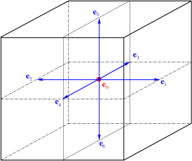
(a) Three-dimensional lattice D3Q7.

            

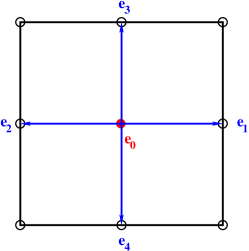
(b) Two-dimensional lattice D2Q5.

Figure 1: Lattices considered in this work. On the left: D3Q7. On the right: D2Q5. The weights of D3Q7 are are $w_{0}=1/4$ and $w_{1,...,6}=1/8$, and its lattice coefficient is $e^{2}=1/4$.The weights of D2Q5 are are $w_{0}=1/3$ and $w_{1,...,4}=1/6$, and its lattice coefficient is $e^{2}=1/3$.

2.2 Equilibrium distribution function adapted to Eq. (1) and BGK collision

For each $t=m\Delta t$ the Boltzmann Equation with BGK collision is (for $i=0,\,...,\,\mathcal{N}$):

$$f_{i}(\mathbf{x}+\mathbf{e}_{i}\Delta x,\,t+\Delta t) =f_{i}(\mathbf{x},\,t)-\frac{1}{\lambda}\left[f_{i}(\mathbf{x},\,t)-f_{i}^{eq}(\mathbf{x},\,t)\right]+w_{i}S_{c}(\mathbf{x},\,t)\Delta t,$$ (8)

where $S_{c}(\mathbf{x},\,t)$ is the source term of Eq. (1) while the $f_{i}^{eq}$ are the entries of a vector called equilibrium distribution function and noted $\bigl{|}\boldsymbol{f}^{eq}\bigr{\rangle}$. The coefficient $\lambda$ is the relaxation rate which relaxes $f_{i}$ towards the equilibrium $f_{i}^{eq}$. The collision operator $\left|\boldsymbol{f}\right\rangle\mapsto\lambda^{-1}\left[\left|\boldsymbol{f}\right\rangle-\left|\boldsymbol{f}^{eq}\right\rangle\right]$ must preserve the total mass, a requirement equivalent to $\sum_{i}f_{i}=\sum_{i}f_{i}^{eq}$. If we set $\boldsymbol{\Lambda}(\mathbf{x})=\lambda^{-1}(\mathbf{x})\mathbf{I}$ ($\mathbf{I}$ being the $\mathcal{N}+1$-dimensional identity matrix), the system of all equations Eq. (8) writes

$$\mathbb{T}\bigl{|}\boldsymbol{f}(\mathbf{x},\,t+\Delta t)\bigr{\rangle}=\bigl{|}\boldsymbol{f}(\mathbf{x},\,t)\bigr{\rangle}-\boldsymbol{\Lambda}(\mathbf{x})\left[\bigl{|}\boldsymbol{f}(\mathbf{x},\,t)\bigr{\rangle}-\bigl{|}\boldsymbol{f}^{eq}(\mathbf{x},\,t)\bigr{\rangle}\right]+\bigl{|}\mathbf{w}\bigr{\rangle}S_{c}(\mathbf{x},\,t)\Delta t$$ (9a)

where operator $$\mathbb{T} \mathbf{e}_{0} \mathbf{e}_{\mathcal{N}}$$ accounts for the translations experienced by the fictitious particles of microscopic displacement vectors , …,  between two successive collision steps, according to

$$\mathbb{T}\bigl{|}\boldsymbol{f}(\mathbf{x},\,t)\bigr{\rangle}=\left(f_{0}(\mathbf{x},\,t),\,f_{1}(\mathbf{x}+\mathbf{e}_{1}\Delta x,\,t),\,...,\,f_{\mathcal{N}}(\mathbf{x}+\mathbf{e}_{\mathcal{N}}\Delta x,\,t)\right)^{T}$$ (9b)

Though partial derivatives are absent from Eqs (8) and (9a)-(9b), they arise when we plug the Taylor expansion of $\mathbb{T}\left|\boldsymbol{f}(\mathbf{x},\,t+\Delta t)\right\rangle-\left|\boldsymbol{f}(\mathbf{x},\,t)\right\rangle$ into Eq. (9a). A standard reasoning of LB literature applies a multiple scale procedure which assumes that there exists a small parameter $\varepsilon$ and a change of variables for $\mathbf{x}$ and $t$ defined by

$$\frac{\partial}{\partial t}=\varepsilon\frac{\partial}{\partial t_{1}}+\varepsilon^{2}\frac{\partial}{\partial t_{2}}\quad\mathrm{and}\quad\frac{\partial}{\partial x_{\mu}}=\varepsilon\frac{\partial}{\partial x^{\prime}_{\mu}}\quad\mathrm{for}\quad\mu=1,\,...,\,d.$$ (10)

This reasoning also assumes bounded derivatives w.r.t. the new variables ($t_{1}$, $t_{2}$, $x^{\prime}_{\mu}$) for all items $\bigl{|}\boldsymbol{f}^{(k)}\bigr{\rangle}$ of the power expansion $\bigl{|}\boldsymbol{f}\bigr{\rangle}=\sum_{k=0}^{+\infty}\varepsilon^{k}\bigl{|}\boldsymbol{f}^{(k)}\bigr{\rangle}$. Collecting items of the order of $\varepsilon^{k}$ for successive integer $k$ returns a sequence of equations among which $C=\langle\mathbf{1}|\boldsymbol{f}^{(0)}\rangle$ approximately solves Eq. (1) in several particular cases (see e.g. [31] and [26] for the ADE and [32, 33] for the phase-field models of crystallization) provided the equilibrium function $\left|\boldsymbol{f}^{eq}\right\rangle$ is appropriately chosen.

A proves that the LB equation approximates Eq. (1) equipped with general $\boldsymbol{\alpha}$ and spherical tensor $\overline{\overline{\mathbf{D}}}=D\overline{\overline{\mathbf{Id}}}$ ($\overline{\overline{\mathrm{\mathbf{Id}}}}$ being the Identity of $\mathbb{R}^{d}$) when the relaxation rate $\lambda$ is related to the diffusion coefficient $D$ by

$$D=e^{2}\left(\lambda-\frac{1}{2}\right)\frac{\Delta x^{2}}{\Delta t}$$ (11)

and the moments of zeroth-, first- and second-order of the equilibrium distribution function $|\boldsymbol{f}^{eq}\rangle$ satisfy

$$\langle\mathbf{1}|\boldsymbol{f}^{eq}\rangle =C$$ (12a)

$$\langle e_{\mu}|\boldsymbol{f}^{eq}\rangle =\frac{\Delta t}{\Delta x}Cu_{\mu}$$ (12b)

$$\langle e_{\mu}e_{\nu}|\boldsymbol{f}^{eq}\rangle =e^{2}\left[p_{\mu}I_{x_{\mu}+}^{2-\alpha_{\mu}}(g_{\mu}C)+(1-p_{\mu})I_{x_{\mu}-}^{2-\alpha_{\mu}}(g_{\mu}C)\right]\delta_{\mu\nu}.$$ (12c)

The equilibrium distribution function

$$\mathbf{|}\boldsymbol{f}^{eq}(\mathbf{x},\,t)\rangle=\left|\boldsymbol{\mathcal{A}}(\mathbf{x},\,t)\right\rangle+\frac{C(\mathbf{x},\,t)}{e^{2}}\frac{\Delta t}{\Delta x}u_{\mu}(\mathbf{x},\,t)\bigl{|}e_{\mu}\mathbf{w}\bigr{\rangle}$$ (13a)

satisfies Eqs (12a)-(12c) if each component $$\mathcal{A}_{i} \left|\boldsymbol{\mathcal{A}}(\mathbf{x},\,t)\right\rangle C \mu=1,\,...,\,d$$ of is a functional of given by (for )

$$\mathcal{A}_{i}(\mathbf{x},\,t)=\begin{cases}C(\mathbf{x},\,t)-w_{0}\sum_{\mu=1}^{d}\left[p_{\mu}I_{x_{\mu}+}^{2-\alpha_{\mu}}(g_{\mu}C)+(1-p_{\mu})I_{x_{\mu}-}^{2-\alpha_{\mu}}(g_{\mu}C)\right]&\mbox{if}\,\,i=0\\ w_{i}\left[p_{\mu}I_{x_{\mu}+}^{2-\alpha_{\mu}}(g_{\mu}C)+(1-p_{\mu})I_{x_{\mu}-}^{2-\alpha_{\mu}}(g_{\mu}C)\right]&\mbox{if}\,\,i=2(\mu-1)+1,\,2(\mu-1)+2\end{cases}$$ (13b)

The second item of Eq. (13a) is a standard element of LBM schemes applied to classical ADE: it accounts for the advective term $$\nabla\cdot(\mathbf{u}C) \left|\boldsymbol{\mathcal{A}}(\mathbf{x},\,t)\right\rangle$$ of Eq. (1). The first item defined by (13b) generalizes to higher dimensions the equilibrium function proposed by [29] for the 1D case.

In the particular case $\boldsymbol{\alpha}=\mathbf{2}$, Eq. (12c) writes $\langle e_{\mu}e_{\nu}|\boldsymbol{f}^{eq\,(0)}\rangle=C\delta_{\mu\nu}$, and $\left|\boldsymbol{\mathcal{A}}(\mathbf{x},\,t)\right\rangle=C\left|\mathbf{w}\right\rangle$ retrieves the equilibrium function commonly used for the classical ADE [26]. Since only the $\mathcal{A}_{i}(\mathbf{x},\,t)$ depend on $\boldsymbol{\alpha}$, simulating the general version of Eq. (1) in any D2Q5 or D3Q7 Lattice Boltzmann code just requires plugging discrete fractional approximations of integrals $I_{x_{\mu}\pm}^{\alpha_{\mu}}g_{\mu}C$ into the equilibrium distribution function according to Eq. (13b). This deserves an algorithm that is described in subsection 2.4.

Eq. (11) intimately links the unique relaxation rate of the BGK LBM to spherical tensor $\overline{\overline{\mathbf{D}}}=D\overline{\overline{\mathbf{Id}}}$ where $D$ may depend on $\mathbf{x}$ and $t$. One relaxation rate still accounts for non-spherical but diagonal $\overline{\overline{\mathbf{D}}}$ if instead of each $g_{\mu}$ in $I_{x_{\mu}\pm}^{\alpha_{\mu}}g_{\mu}C$ we set $h_{\mu}g_{\mu}$ with $h_{\mu}$ such that $D_{\mu\mu}=e^{2}\left(\lambda-\frac{1}{2}\right)h_{\mu}\Delta x^{2}/\Delta t$ provided $\overline{\overline{\mathbf{D}}}$ does not depend on $\mathbf{x}$. Nevertheless, even if the latter condition is satisfied non-trivial off-diagonal entries of $\overline{\overline{\mathbf{D}}}$ remain excluded. This fosters us considering in Section 2.3 more flexible MRT collision rules still based on the e.d.f. defined by Eqs (13a)-(13b), but involving more freedom degrees. These collision rules moreover help us damping instabilities caused by large velocity $\mathbf{u}$ even with diagonal diffusion tensor.

2.3 MRT collision operator

The MRT collision operator [34, 35] $\mathbf{M}^{-1}\boldsymbol{\Lambda}(\mathbf{x})\mathbf{M}\left[\left|\boldsymbol{f}(\mathbf{x},\,t)\right\rangle-\left|\boldsymbol{f}^{eq}(\mathbf{x},\,t)\right\rangle\right]$ includes invertible $(\mathcal{N}+1)\times(\mathcal{N}+1)$ matrices $\mathbf{M}$ and $\boldsymbol{\Lambda}$, and here the above defined equilibrium function is still used. The LB equation (9a) is replaced by

$$\mathbb{T}\bigl{|}\boldsymbol{f}(\mathbf{x},\,t+\Delta t)\bigr{\rangle}=\bigl{|}\boldsymbol{f}(\mathbf{x},\,t)\bigr{\rangle}-\mathbf{M}^{-1}\boldsymbol{\Lambda}(\mathbf{x})\mathbf{M}\left[\bigl{|}\boldsymbol{f}(\mathbf{x},\,t)\bigr{\rangle}-\bigl{|}\boldsymbol{f}^{eq}(\mathbf{x},\,t)\bigr{\rangle}\right]+\bigl{|}\mathbf{w}\bigr{\rangle}S_{c}(\mathbf{x},\,t)\Delta t,$$ (14)

in which matrix $\mathbf{M}$ represents a change of basis. In MRT collision rule the latter associates to each $\left|\boldsymbol{f}\right\rangle$ a set of $\mathcal{N}+1$ independent moments equivalent to scalar products of $\left|\boldsymbol{f}\right\rangle$ by independent elements of $\mathbb{R}^{\mathcal{N}+1}$ including $\left|\mathbf{1}\right\rangle$, the $\bigl{|}e_{\mu}\bigr{\rangle}$ and combinations of products of these vectors. In the new basis, the $d+1$ first new coordinates of $\left|\boldsymbol{f}\right\rangle$ are the total mass $\left\langle\mathbf{1}|\boldsymbol{f}\right\rangle$ (a conserved quantity) and the $\bigl{\langle}\boldsymbol{f}\bigr{|}e_{\mu}\bigr{\rangle}$, proportional to fictive particle fluxes in the $d$ physical directions. These $d+1$ first rows turn out to be mutually orthogonal. Reference [26] suggests complementing them with $\mathcal{N}-d$ rows associated to second order moments related to kinetic energy $\left|\mathbf{e}^{2}\right\rangle=\sum_{\mu=1}^{d}\bigl{|}e_{\mu}e_{\mu}\bigr{\rangle}$ and to other linear combinations of the $\bigl{|}e_{\mu}e_{\mu}\bigr{\rangle}$ with $\mu<d$, mutually orthogonal and orthogonal to the $d+1$ first rows. Any linear combination of these vectors is suitable if all rows are mutually orthogonal. This requirement, justified by accumulated experience, seems necessary to achieve numerical stability when $\mathbf{u}$ is different from zero. It is satisfied by several configurations among which we choose the ones suggested by [26]:

$$\mathbf{M}=\left(\begin{array}[]{ccccccc}1&1&1&1&1&1&1\\ 0&1&-1&0&0&0&0\\ 0&0&0&1&-1&0&0\\ 0&0&0&0&0&1&-1\\ 6&-1&-1&-1&-1&-1&-1\\ 0&2&2&-1&-1&-1&-1\\ 0&0&0&1&1&-1&-1\end{array}\right)\;\mathrm{or}\;\;\mathbf{M}=\left(\begin{array}[]{ccccc}1&1&1&1&1\\ 0&1&-1&0&0\\ 0&0&0&1&-1\\ 4&-1&-1&-1&-1\\ 0&1&1&-1&-1\end{array}\right),$$ (15)

for D3Q7 or D2Q5 respectively. The $\boldsymbol{\Lambda}(\mathbf{x})$ matrix associated to the D3Q7 lattice is defined by its inverse

$$\boldsymbol{\Lambda}^{-1}(\mathbf{x})=\left(\begin{array}[]{ccccccc}\lambda_{0}(\mathbf{x})&0&0&0&0&0&0\\ 0&\lambda_{11}(\mathbf{x})&\lambda_{12}(\mathbf{x})&\lambda_{13}(\mathbf{x})&0&0&0\\ 0&\lambda_{21}(\mathbf{x})&\lambda_{22}(\mathbf{x})&\lambda_{23}(\mathbf{x})&0&0&0\\ 0&\lambda_{31}(\mathbf{x})&\lambda_{32}(\mathbf{x})&\lambda_{33}(\mathbf{x})&0&0&0\\ 0&0&0&0&\lambda_{4}(\mathbf{x})&0&0\\ 0&0&0&0&0&\lambda_{5}(\mathbf{x})&0\\ 0&0&0&0&0&0&\lambda_{6}(\mathbf{x})\end{array}\right)$$ (16)

whose elements are relaxation rates. In dimension two with D2Q5, we just skip elements $\lambda_{3\mu}$ and $\lambda_{\mu 3}$ and replace $\lambda_{5}$ and $\lambda_{6}$ by $\lambda_{3}$. In both cases, we call $\overline{\overline{\boldsymbol{\lambda}}}$ the $d\times d$ matrix of elements $\lambda_{\mu\nu}$.

Assuming $\Delta t\sim\Delta x^{2}$, the reference [26] proves that the moment of zeroth-order $C=\langle\mathbf{1}|\boldsymbol{f}\rangle$ deduced from Eqs (14), (16), or (15) solves the anisotropic ADE (i.e. Eq. (1) with $\boldsymbol{\alpha}=\mathbf{2}$) within an error of the order of $\varepsilon^{2}$ provided diffusion tensor and relaxation parameters satisfy

$$\overline{\mathbf{\overline{D}}}(\mathbf{x})=e^{2}\left(\overline{\overline{\boldsymbol{\lambda}}}(\mathbf{x})-\frac{1}{2}\overline{\overline{\mathrm{\mathbf{Id}}}}\right)\frac{\Delta x^{2}}{\Delta t}$$ (17)

which generalizes Eq. (11). A.2 extends this statement to general $\boldsymbol{\alpha}$. Eq. (17) relates the elements $\lambda_{\mu\nu}(\mathbf{x})$ of matrix $\boldsymbol{\Lambda}^{-1}(\mathbf{x})$ ($\mu,\,\nu=1,\,...,\,d$) to the generalized diffusion tensor, and $\lambda_{0}(\mathbf{x})$ (applied on the conserved quantity) has no effect. Section 3.3 demonstrates that the diagonal elements $\lambda_{\mu}(\mathbf{x})$ with $\mu=d+1,\,...,\,\mathcal{N}$ can be viewed as additional freedom degrees influencing the stability and the accuracy of the algorithm.

2.4 Computation of discrete integrals

Updating the discrete equilibrium function at each time step requires discrete fractional integrals, in BGK as well as in MRT setting. Accurately discretizing the fractional integrals $I_{x_{\mu}\pm}^{2-\alpha_{\mu}}$ involved in the $\mathcal{A}_{i}(\mathbf{x},\,t)$ significantly improves the efficiency of LBM schemes applied to Eq. (1). Discrete schemes are available for one-dimensional fractional integrals of any continuous function $f(x)$ of a real variable $x\in[0,\,N\Delta x]$. Approximations of the order of $\Delta x$ may be sufficient in the one-dimensional case as in Ref. [29]. Since higher $d$ dimension fosters us avoiding too small mesh, we disregard discrete algorithms using step functions to interpolate $f(x)$, and prefer those of [36] which stem from the trapezoidal rule and return errors of the order of $\Delta x^{2}$:

$$I_{n\Delta x+}^{\gamma}f\approx\frac{\Delta x^{\gamma}}{\Gamma(2+\gamma)}\sum_{l=0}^{n}f(l\Delta x)c_{ln}^{+}(\gamma)\quad\quad I_{n\Delta x-}^{\gamma}f\approx\frac{\Delta x^{\gamma}}{\Gamma(2+\gamma)}\sum_{l=n}^{N}f(l\Delta x)c_{ln}^{-}(\gamma,\,N).$$ (18)

These equations need the Gamma function for which an intrinsic Fortran 2008 function exists, and coefficients $c_{ln}^{+}(\gamma)$ and $c_{ln}^{-}(\gamma,\,N)$ are defined by:

$$c_{ln}^{+}(\gamma)=\begin{cases}(1+\gamma)n^{\gamma}-n^{\gamma+1}+(n-1)^{\gamma+1}&\textrm{for}\,\,l=0,\\ (n-l+1)^{\gamma+1}-2(n-l)^{\gamma+1}+(n-l-1)^{\gamma+1}&\textrm{for}\,\,0<l<n,\\ 1&\textrm{for}\,\,l=n\end{cases}$$ (19a)

and:

$$c_{ln}^{-}(\gamma,\,N)=\begin{cases}(1+\gamma)(N-n)^{\gamma}-(N-n)^{\gamma+1}+(N-n-1)^{\gamma+1}&\textrm{for}\,\,l=N,\\ (l-n+1)^{\gamma+1}-2(l-n)^{\gamma+1}+(l-n-1)^{\gamma+1}&\textrm{for}\,\,n<l<N\\ 1&\textrm{for}\,\,l=n\end{cases}$$ (19b)

For $d>1$ and each $\mu$, we use Eq. (18) in $(I_{x_{\mu}\pm}^{\gamma_{\mu}}C)(\mathbf{x})$ which is an integral of the form $(I_{x_{\mu}\pm}^{\gamma_{\mu}}f)(x_{\mu})$ if we set $f(x_{\mu})\equiv C(\mathbf{x})$ in which we fix all coordinates of $\mathbf{x}$ of rank different from $\mu$. For each $\mathbf{x}=(x_{1},\,...,\,x_{d})$ belonging to the domain $\Omega=\Pi_{\mu=1}^{d}[\ell_{\mu},\,L_{\mu}=\ell_{\mu}+N_{\mu}\Delta x]$, we set $x_{\mu}=\ell_{\mu}+n\Delta x$ and yield

$$(I_{x_{\mu}+}^{\gamma_{\mu}}C)(\mathbf{x})=\frac{\Delta x^{\gamma_{\mu}}}{\Gamma(2+\gamma_{\mu})}\sum_{l=0}^{n}C(\mathbf{y}_{l})c_{ln}^{+}(\gamma_{\mu}),\quad\quad(I_{x_{\mu}-}^{\gamma_{\mu}}C)(\mathbf{x})=\frac{\Delta x^{\gamma_{\mu}}}{\Gamma(2+\gamma_{\mu})}\sum_{l=n}^{N_{\mu}}C(\mathbf{y}_{l})c_{ln}^{-}(\gamma_{\mu},\,N_{\mu})$$ (20)

where $\mathbf{y}_{l}$ has the same meaning as $\mathbf{y}$ in Eq. (3). For instance, in the particular case $d=3$, $\mathbf{y}_{l}=(\ell_{1}+l\Delta x,\,x_{2},\,x_{3})$ if $\mu=1$, $\mathbf{y}_{l}=(x_{1},\,\ell_{2}+l\Delta x,\,x_{3})$ if $\mu=2$ and $\mathbf{y}_{l}=(x_{1},\,x_{2},\,\ell_{3}+l\Delta x)$ if $\mu=3$.

Because fractional integrals are non-local, updating the equilibrium function at each computing step needs the complete description of the concentration field in $\Omega$. Parallel computing would need specific programming effort in this case.

2.5 Boundary conditions and algorithm

Here we consider homogeneous and non-homogeneous Dirichlet boundary conditions at the boundary of domain $\Omega$ limited by hyperplanes of inward normal unit vectors $\mathbf{e}_{b}$ with $b=1,\,...,\,\mathcal{N}$. At each node $\mathbf{x}$ of such boundary, after the collision stage, each displacement stage derives from Eq. (9b) all the components of the distribution function $\bigl{|}\boldsymbol{f}\bigr{\rangle}$ except $f_{b}$. This accounts for the possible asymmetry of the equilibrium function since the collision stage has been performed. Imposing concentration $C_{0}$ is equivalent to update the unknown function

$$f_{b}=C_{0}-\sum_{i\neq b}^{\mathcal{N}}f_{i}.$$ (21)

For instance, assuming $b=1$ with a three-dimensional D3Q7 lattice at point $\mathbf{x}=(\ell_{1},\,x_{2},\,x_{3})^{T}$, the unknown distribution function $f_{1}$ is given by $f_{1}=C_{0}-\sum_{i\neq 1}^{\mathcal{N}}f_{i}=C_{0}-f_{0}-f_{2}-f_{3}-f_{4}-f_{5}-f_{6}$. This method is also applied when the concentration $C_{0}$ varies with position and time (see Section 3.4).

The main stages of the above described LBM scheme are summarized in Algorithm 1. Only the first two stages of the time loop differ from standard LBM applied to classical ADE because updating the equilibrium distribution function $\bigl{|}\boldsymbol{f}^{eq}\bigr{\rangle}$ requires fractional integrals $I_{x_{\mu}\pm}^{2-\alpha_{\mu}}(g_{\mu}C)$ discretized according to Section 2.4. Regarding initializations, the third item is applicable to MRT LBM only. Parameters $\lambda_{\mu}$ with $\mu=d+1,\,...,\,\mathcal{N}$ achieving stability and accuracy of MRT LBM schemes approximating the fractional ADE may belong to a subset of those adapted to the classical case $\boldsymbol{\alpha}=\boldsymbol{2}$. Choosing these parameters was found necessary at large Péclet numbers in the numerical experiments described in Section 3.

Initializations

1. Define time step $\Delta t$, space step $\Delta x$, moving vectors $\mathbf{e}_{i}$, weights $w_{i}$ and lattice coefficient $e^{2}$.

2. Being given $D$ (or $D_{\mu\nu}$), calculate the relaxation rates $\lambda$ (or $\lambda_{\mu\nu}$) with Eq. (11) (or Eq. (17)).

3. Choose parameters $\lambda_{\mu}$ ($\mu=d+1,\,...,\,\mathcal{N}$) in MRT case.

4. Read or define the initial conditions $C(\mathbf{x},\,0)$, and $\mathbf{u}(\mathbf{x},\,0)$.

Start of time loop

1. For each $\mu=1,\,...,\,d$, calculate the fractional term $\left[p_{\mu}I_{x_{\mu}+}^{2-\alpha_{\mu}}(g_{\mu}C)+(1-p_{\mu})I_{x_{\mu}-}^{2-\alpha_{\mu}}(g_{\mu}C)\right]$.

2. Calculate the e.d.f. $\bigl{|}\boldsymbol{f}^{eq}\bigr{\rangle}$ defined by Eqs. (13a)-(13b). This gives us the right-hand side of Eqs (9a) or (14)

3. Apply operator $\mathbb{T}^{-1}$ (displacement) to this right-hand side and get $\left|\boldsymbol{f}(\mathbf{x},\,t+\Delta t)\right\rangle$

4. Update the boundary conditions with Eq. (21).

5. Calculate the new concentration $C(\mathbf{x},\,t)=\bigl{\langle}\mathbf{1}\bigr{|}\boldsymbol{f}\bigr{\rangle}$.

End of time loop

Algorithm 1 LBM algorithm for fractional ADE.

3 LBM-FADE validations

Numerical algorithms proposed to solve partial differential equations can be checked by comparing with exact solutions, or with numerical solutions issued of other approaches. Analytical solutions are available for Eq. (1) involving general $\boldsymbol{\alpha}$ provided the skewness parameter $\boldsymbol{p}$ takes the value $\mathbf{1}$ or $\mathbf{0}$ with, moreover, specific source term $S_{c}$ and initial data. Though Eq. (1) with $S_{c}=0$ constitutes an important simple case, it does not have exact solutions in bounded domains. However, in this case Eq. (1) equipped with spatially homogeneous coefficients rules the evolution of the probability density function (p.d.f) of a wide class of stochastic processes described in subsection 3.1. Sampling sufficiently many trajectories of such process yields random walk approximation of Eq. (1). Subsections 3.2 and 3.3 compare issues of the LBM scheme described in Section 2 with such random walks when $\mathbf{u}=\mathbf{0}$ and $\mathbf{u}\neq\mathbf{0}$ respectively. Subsection 3.4 considers anisotropic and space-dependent diffusion tensor such that Eq. (1) has an exact solution which is compared with LBM simulation. Subsection 3.5 shows that the simulation adapts to slightly different (still fractional) $\boldsymbol{\mathcal{F}}^{\boldsymbol{\alpha}\boldsymbol{p}\boldsymbol{g}}(C)$ in Eq. (1). Hence, exact solutions and random walks help us to validate LBM schemes in complementary situations.

3.1 Fractional random walks

Eq. (1) rules the evolution of stochastic processes in $\mathbb{R}^{d}$, and in bounded domains under some conditions. Though comparisons with numerical LBM simulations correspond to the latter case, we start with unconstrained random walks and briefly comment the role of the several parameters of Eq. (1).

Equation (1) and random walks in $\mathbb{R}^{d}$

Eq. (1) with $\boldsymbol{\alpha}=\mathbf{2}$ is the ADE, and random walks are commonly used to simulate the solutions of this equation. To recall the principle of this method we assume for simplicity a diagonal tensor $\overline{\overline{\mathbf{D}}}$ and a vector $\boldsymbol{g}$ independent of $\mathbf{x}$, here equal to $\boldsymbol{1}$. We consider a $d$-dimensional random variable $\mathbf{X}(0)$ of probability density function $\Phi$, and call $\mathbf{B}(t)$ the standard $d$-dimensional Brownian motion, and $\overline{\overline{\mathbf{D^{\prime}}}}$ the tensor of entries $D^{\prime}_{\mu\nu}=(D_{\mu\mu}g_{\mu})^{1/2}\delta_{\mu\nu}$. Moreover, for each stochastic process $\mathbf{Y}(t)$ we call $\delta\mathbf{Y}(t,\,t+\delta t)$ its increment $\mathbf{Y}(t+\delta t)-\mathbf{Y}(t)$. With these notations, the ADE with the initial condition $\Phi$ rules the p.d.f. of the stochastic process $\mathbf{X}(t)$ that starts from $\mathbf{X}(0)$ and has increments satisfying

$$\delta\mathbf{X}(t,\,t+\delta t)=\mathbf{u}(\mathbf{X}(t))\delta t+\overline{\overline{\mathbf{D^{\prime}}}}\delta\mathbf{B}(t,\,t+\delta t)$$ (22)

for $\delta t>0$ [37]. For each $t\geq 0$ and each $\delta t>0$, it turns out that $\delta\mathbf{B}(t,\,t+\delta t)$ is distributed as $\sqrt{2\delta t}\mathbf{G}$, where $\mathbf{G}$ is a random variable of $\mathbb{R}^{d}$ with mutually independent standard Gaussian entries, also independent of what happened before $t$. Sampling $\mathcal{N}_{RW}$ independent trajectories of $\mathbf{X}(t)$ by applying Eq. (22) to successive intervals of fixed step $\delta t$ [14] yields histograms that approximate the p.d.f. of $\mathbf{X}(t)$, i.e. the solution of Eq. (1) started from $\Phi$, provided $\boldsymbol{\alpha}=\mathbf{2}$. Increasing $\mathcal{N}_{RW}$ improves the accuracy of such random walk approximation, still valid when $\boldsymbol{g}$ depends on $\mathbf{x}$ if we plug $g_{\mu}(X(t))$ instead of $g_{\mu}$ in the entries of $\overline{\overline{\mathbf{D^{\prime}}}}$ that appear in Eq. (22). Note that this is not true if $\overline{\overline{\mathbf{D}}}$ is allowed to depend on $\mathbf{x}$ [14]: this fact motivates separating $\overline{\overline{\mathbf{D}}}$ and $\boldsymbol{g}$ in Eq. (1). Decreasing $\delta t$ is useful only when $\mathbf{u}$ or $\boldsymbol{g}$ do depend on space, in unbounded domain.

Actually, Eq. (22) only describes a particular case of more general $\mathbf{X}(t)$ defined for $t\geq 0$ and $\delta t>0$ by

$$\delta\mathbf{X}(t,\,t+\delta t)=\mathbf{u}(\mathbf{X}(t))\delta t+\overline{\overline{\mathbf{D^{\prime}}}}\delta\mathbf{L}_{\boldsymbol{\alpha},\boldsymbol{\beta}}(t,\,t+\delta t)$$ (23)

which is very similar to Eq. (22), except that $D^{\prime}_{\mu\nu}=(D_{\mu\mu}g_{\mu})^{1/\alpha_{\mu}}\delta_{\mu\nu}$ and the Brownian motion $\mathbf{B}$ is replaced by the stable $d$-dimensional random process $\mathbf{L}_{\boldsymbol{\alpha},\boldsymbol{\beta}}$. The latter is completely determined by two sets of parameters encapsulated in two vectors, namely $\boldsymbol{\alpha}$ defined in Section 1, and another vector $\boldsymbol{\beta}$ of $\mathbb{R}^{d}$ whose entries $\beta_{\mu}$ belong to $[-1,\,1]$. As $\delta\mathbf{B}(t,\,t+\delta t)$ above, $\delta\mathbf{L}_{\boldsymbol{\alpha},\boldsymbol{\beta}}(t,\,t+\delta t)$ has $d$ mutually independent components $\mathbf{b}_{\mu}\cdot\delta\mathbf{L}_{\boldsymbol{\alpha},\boldsymbol{\beta}}$ that are independent of what happened before instant $t$. For each $\delta t>0$ they satisfy

$$\mathbf{b}_{\mu}\cdot\delta\mathbf{L}_{\boldsymbol{\alpha},\boldsymbol{\beta}}(t,\,t+\delta t)\overset{d}{=}\left(-\cos\frac{\pi\alpha_{\mu}}{2}\delta t\right)^{1/\alpha_{\mu}}S(\alpha_{\mu},\,\beta_{\mu})$$ (24)

where symbol $\overset{d}{=}$ links equally distributed random variables. Moreover, the one-dimensional stable random variable $S(\alpha_{\mu},\,\beta_{\mu})$ described in B.1 is entirely determined by its stability exponent $\alpha_{\mu}$ and its skewness parameter $\beta_{\mu}$. Since $S(\alpha_{\mu},\,\beta_{\mu})$ is Gaussian in the limit case $\alpha_{\mu}=2$ (whatever the value of $\beta_{\mu}$), we retrieve $\mathbf{B}$ in $\mathbf{L}_{\boldsymbol{2},\boldsymbol{\beta}}$. With these notations, the p.d.f of $\mathbf{X}(t)$ defined by Eq. (23) satisfies Eq. (1) in $\mathbb{R}^{d}$ provided $\boldsymbol{\beta}=2\boldsymbol{p}-\mathbf{1}$ according to [12, 13].

We sample $\mathbf{X}(t)$ by applying Eqs (23)-(24) with prescribed $\delta t$, and the density of the sample approximately solves Eq. (1) as in the diffusive case. This needs sampling many values of the $S(\alpha_{\mu},\,\beta_{\mu})$: each one is given by applying algebraic formulas of [38] to a pair of independent random numbers which are drawn from two uniform distributions. This procedure works for general initial data equivalent to the p.d.f. $\Phi$ of $\mathbf{X}(0)$. When we assume spatially homogeneous parameters, replacing $t$ by $0$ and $\delta t$ by $t$ in Eqs. (23)-(24) returns the distribution of $\mathbf{X}(t)$ in one shot. However, spatially inhomogeneous parameters or bounded domain require small $\delta t$ in Eqs. (23)-(24).

Influence of parameters $\boldsymbol{\alpha}$ and $\boldsymbol{\beta}$

The stable process $\mathbf{L}_{\boldsymbol{\alpha},\boldsymbol{\beta}}$ defined by Eq. (24) exhibits super-diffusion in each direction $x_{\mu}$ such that $\alpha_{\mu}<2$. This means infinite second moment for its projection on $\mathbf{b}_{\mu}$, equivalent to large displacements significantly more probable than for $\alpha_{\mu}=2$. More specifically, the density of $S(\alpha_{\mu}<2,\,\beta_{\mu})$ is illustrated by Fig. 9 and falls off as $x^{-\alpha_{\mu}-1}$ while that of $S(\alpha_{\mu}=2,\,\beta_{\mu})$ decays exponentially.

The second parameter $\beta_{\mu}$ in $S(\alpha_{\mu},\,\beta_{\mu})$ quantifies the skewness degree of the distribution of this random variable (see Fig. 9), which also rules the displacements of $\mathbf{L}_{\boldsymbol{\alpha},\boldsymbol{\beta}}$ in $x_{\mu}$ direction. Yet, stability exponent $\alpha_{\mu}$ approaching $2$ decreases this influence which becomes evanescent in the limit case $\alpha_{\mu}=2$. While Brownian motion has symmetrically distributed displacements in each direction, for $\alpha_{\mu}<2$ the displacements of $\mathbf{L}_{\boldsymbol{\alpha},\boldsymbol{\beta}}$ and $\mathbf{X}(t)$ in $\mathbf{b}_{\mu}$ direction are symmetric only if $\beta_{\mu}=0$. Moreover, larger positive $\beta_{\mu}$ magnify large positive jumps and decrease large negative jumps. Nevertheless the average remains equal to $0$. This causes most probable jumps to be negative for $\beta_{\mu}>0$ (see Fig. 9), and in the limit case $\beta_{\mu}=1$, large negative jumps occur even more scarcely than in Brownian motion.

Random walks in bounded domain and equation associated with Dirichlet boundary conditions

The above described link between $\mathbf{X}(t)$ and Eq. (1) in $\Omega=\mathbb{R}^{d}$ persists in bounded domain provided we consider boundary conditions equivalent to restrictions imposed to the sample paths of $\mathbf{X}(t)$ [21, 39]. However, most boundary problems associated with space-fractional p.d.es remain still open. It is only in specific cases that we actually know slight modifications that transform the sample paths of $\mathbf{X}(t)$ into the ones of a closely related random walk whose p.d.f satisfies Eq. (1) and prescribed boundary conditions. This occurs in the simple case of homogeneous Dirichlet conditions [40, 41, 42, 43] which we use for checks. Associating Eq. (1) with non-homogeneous Dirichlet conditions returns problems whose well-posedness is not assessed: solutions do exist but uniqueness apparently depends on how we interpret these boundary conditions in the case of space-fractional equations [43]. We disregard here Neumann conditions because it is only in too miscellaneous cases that they have been proved to correspond to sample paths transformations compatible with density satisfying Eq. (1). Just note that Neumann conditions for space-fractional p.d.es as Eq. (1) involve fractional derivatives of order $\alpha_{\mu}-1$ [21, 44], as the dispersive flux driven by stable process [20].

Assuming space-independent parameters, we detail in B.2 why Eq. (1) associated to homogeneous Dirichlet conditions at the boundary of a rectangle rules the evolution of the p.d.f of $\mathbf{X}^{\Omega}(t)$, a process derived from $\mathbf{X}(t)$ by killing each sample path at its first exit time $\tau_{\Omega}$ [40]. From a practical point of view, each sample path of $\mathbf{X}$ determines one value of the random variable $\tau_{\Omega}$ and one sample path of $\mathbf{X}^{\Omega}$ composed of all its positions before time $\tau_{\Omega}$. The remainder of the sample path of $\mathbf{X}$ does not contribute to that of $\mathbf{X}^{\Omega}$, even if it returns to $\Omega$ after time $\tau_{\Omega}$. Consequently, good approximations to sample path of $\mathbf{X}^{\Omega}$ need small $\delta t$ in Eq. (23) which would not be necessary if no boundary condition were imposed with spatially uniform parameters. Here we use random walks to approximate the p.d.f. of $\mathbf{X}^{\Omega}(t)$ which we deduce from an histogram of a sample. Therefore, we consider $\delta t$ small enough when decreasing $\delta t$ does not modify the histogram. This criterion is satisfied by $\delta t\leq 0.001$ in all presented comparisons.

3.2 Comparisons between LBM and RW for $\mathbf{u}=\mathbf{0}$

Without advection ($\mathbf{u}=\mathbf{0}$) and when the diffusion tensor is isotropic ($\overline{\overline{\mathbf{D}}}=D\overline{\overline{\mathbf{Id}}}$), BGK and MRT collision rules return quite comparable approximations to Eq. (1). This is what we check in this subsection by comparing LBM with random walk simulations in dimensions $d=2$ and $d=3$ with spatially uniform coefficients. Validations are presented for three sets of parameters that exemplify the strange behaviors included in Eq. (1), and associated to symmetric or skewed super-diffusion. Moreover, all these random walk simulations are started from a sample of the $d$-dimensional Gaussian random variable $\mathbf{X}(0)$ of standard deviation $\sigma_{0}$, and centered at point $\mathbf{x}^{s}$ of coordinates $x_{\mu}^{s}$. The p.d.f. of $\mathbf{X}(0)$ is the standard Gaussian hill

$$C(\mathbf{x},\,0)=\frac{C_{0}}{(2\pi\sigma_{0}^{2})^{d/2}}\exp\left[-\frac{1}{2\sigma_{0}^{2}}\sum_{\mu=1}^{d}(x_{\mu}-x_{\mu}^{s})^{2}\right],$$ (25)

a smooth initial condition suited for LBM, and approximated by the distribution of the sample when $\mathcal{N}_{RW}$ is large enough. Choosing $\sigma_{0}$ small concentrates this initial condition near point $\mathbf{x}^{s}$. For all simulations of this paper, we set $\sigma_{0}=0.002$ and $C_{0}=5$.

The two-dimensional validations 1 and 2 assume square domain $\Omega$ ($\ell_{1}=\ell_{2}=0$, $L_{1}=L_{2}=2$) and the initial condition is located at domain center: $\mathbf{x}^{s}=(1,\,1)^{T}$. Then, the p.d.f. of $\mathbf{X}^{\Omega}(t)$ satisfies Eq. (1). It is of the form of $C(x_{1},\,x_{2},\,t)=P_{1}(x_{1},\,t)P_{2}(x_{2},\,t)$ where each $P_{\mu}$ solves the one-dimensional version of Eq. (1) in $]\ell_{\mu},\,L_{\mu}[$, according to B.2. We moreover assume $\overline{\overline{\mathbf{D}}}=0.5\overline{\overline{\mathbf{Id}}}$ and $\boldsymbol{g}=\mathbf{1}$.

Validation 1: the effect of $\alpha_{\mu}$ when $\beta_{\mu}=0$

With parameters $\boldsymbol{\alpha}=(1.5,\,1.99)^{T}$ and $\boldsymbol{\beta}=\mathbf{0}$, the process $\mathbf{X}^{\Omega}$ defined in Section 3.1 accumulates symmetric displacements. This is equivalent to integrals $I_{x_{\mu}\pm}^{2-\alpha_{\mu}}$ of equal weights in Eq. (2). Here with $\mathbf{u}=\mathbf{0}$, we see on Fig. 2 that the maximum of the solution to Eq. (1) stays immobile. Counting the sample paths that leave $\Omega$ reveals that most of them exit through boundaries $x_{1}=\ell_{1}$ and $x_{1}=L_{1}$, due to large displacements more probable in $x_{1}$-direction because of $\alpha_{1}<\alpha_{2}$. At times $t$ satisfying $D_{\mu\mu}g_{\mu}t<1$ the left panel of Fig. 2a exhibits profiles $C(x_{1},\,x_{2}^{s},\,t)$ (in $x_{1}$-direction where super-diffusion occurs). They are thinner than profiles $C(x_{1}^{s},\,x_{2},\,t)$ represented on the right and describing the variations of $C$ in $x_{2}$-direction where diffusion is almost normal. Actually, this agrees with Eq. (24) though this equation is only exact in unbounded domain. At times satisfying $D_{\mu\mu}g_{\mu}t\geq 1$ (not represented here) the information included in this equation is no longer valid for the two profiles which become similar to each other, but small because almost all the sample paths have left $\Omega$. LBM and random walk simulation agree fairly well even in the neighborhood of the boundaries magnified on Fig.2b, with space and time steps $\Delta x=0.02$ and $\Delta t=10^{-4}$. This necessitates $100^{2}$ nodes in the considered domain, and $10^{3}$ time steps completed in $9$ minutes on simple core desktop workstation.

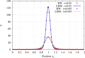
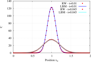
(a) Narrow peak caused by super-diffusion at early times. Left: profiles $C(x_{1},\,x_{2}^{s},\,t)$ in $x_{1}$-direction along which super-diffusion occurs at times $t_{1}=0.01$ and $t_{2}=0.045$. Right: $C(x_{1}^{s},\,x_{2},\,t)$ profiles at the same times in $x_{2}$-direction along which diffusion is almost normal.

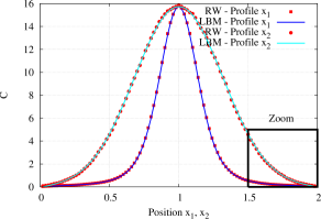
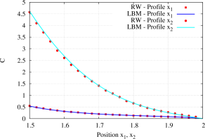
(b) Left: global view of $x_{1}$- and $x_{2}$-profiles at $t_{3}=0.1$, showing the region magnified at the right. Right: magnification near right boundary. At time $t_{3}=0.1$, profiles in $x_{1}$-direction exhibit heavier tails than earlier, and the peak near the maximum is still narrow compared with $C(x_{1}^{s},\,x_{2},\,t_{3})$.

Figure 2: Solutions of the 2D Eq. (1) with symmetric integrals ($\boldsymbol{p}=\boldsymbol{1/2}$) w.r.t. each coordinate. The stability parameter is equivalent to super-diffusion only in $x_{1}$-direction: $\boldsymbol{\alpha}=(1.5,\,199)^{T}$. LBM and RW return indistinguishable approximations, even near the boundaries.

Validation 2: non-symmetric super-diffusion

For $\beta_{\mu}\neq 0$ and $\alpha_{\mu}$ strictly between $1$ and $2$, $S(\alpha_{\mu},\,\beta_{\mu})$ is not symmetric and the sign of its most probable value is that of $-\beta_{\mu}$, though the average is zero. The same holds for $\mathbf{b}_{\mu}\cdot\mathbf{L}_{\boldsymbol{\alpha},\boldsymbol{\beta}}$ whose most probable value has a modulus that increases with time due to Eq. (24). Here with $\mathbf{u}=\mathbf{0}$, the most probable value of $\mathbf{X}^{\Omega}$ (equivalent to the maximum of the solution $C$ to Eq. (1)) exhibits the same behavior if the initial data $\Phi$ is localized far from the boundaries, and at times such that a small amount of tracer has left $\Omega$. Fig. 3a (obtained with $\boldsymbol{\alpha}=\mathbf{1.2}$ and $\boldsymbol{p}=(0.35,\,0.5)^{T}$) illustrates the shift of this maximum and exhibits left tail slightly thicker than right tail. This is due to $p_{1}<0.5$ that makes large negative displacements in $x_{1}$-direction more probable. Fig. 3b reveals that BGK collision rule achieves perfect agreement with random walk even near the boundary, here with $\Delta x=0.01$ and $\Delta t=5\times 10^{-5}$ necessitating $200^{2}$ nodes and $2\times 10^{4}$ times steps (to reach $t=1$) completed in $16.89$ hours by the above mentioned workstation. Fig. 4a represents the evolution of the solute plume that corresponds to Fig. 4b: though $\mathbf{u}=\mathbf{0}$, the plume center shifts to the right in $x_{1}$-direction. Nevertheless the iso-levels of $C$ extend farther to the left than to the right in the direction of $x_{1}$. They show larger curvature than if $p_{1}$ and $p_{2}$ were equal (see [13]), and are reminiscent of anisotropic diffusion though here $\overline{\overline{\mathbf{D}}}$ is spherical with $\alpha_{1}=\alpha_{2}$.

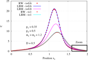
(a) $C(x_{1},\,x_{2}^{s},\,t)$ profiles at $t_{1}=0.6$ (blue), $t_{2}=0.8$ (magenta) and $t_{3}=1$ (cyan).

      

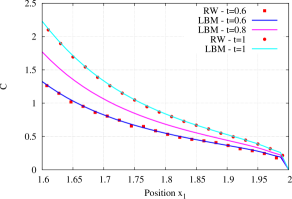
(b) Magnification of the neighborhood of the right boundary.

Figure 3: $C(x_{1},\,1,\,t)$ Profiles of solutions of the 2D Eq. (1) equipped with the same stability parameter in all directions and with non-symmetric integrals in $x_{1}$-direction only: $\boldsymbol{p}=(0.35,\,0.5)^{T}$ and $\boldsymbol{\alpha}=\boldsymbol{1.2}$. LBM and RW return indistinguishable approximations, even near the right boundary where the solution decreases especially rapidly due to $\alpha_{1}$ and to skewness.

$t=0.05$	$t=0.2$	$t=0.6$	$t=1$

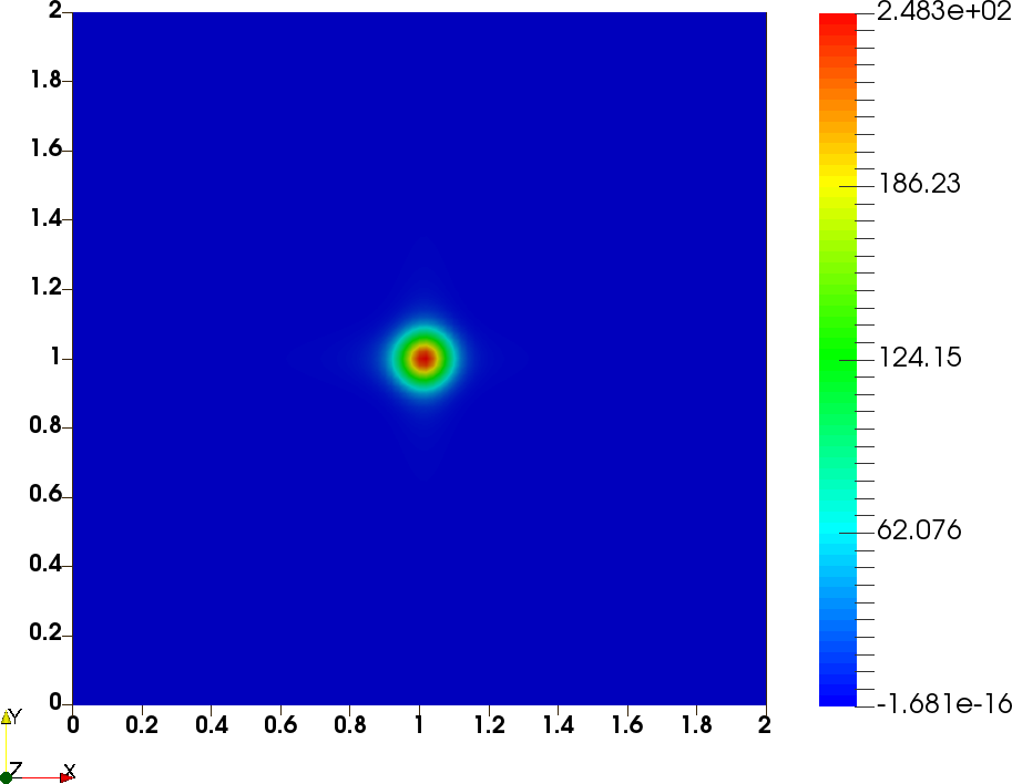
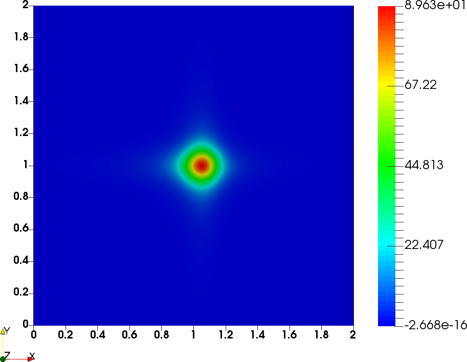
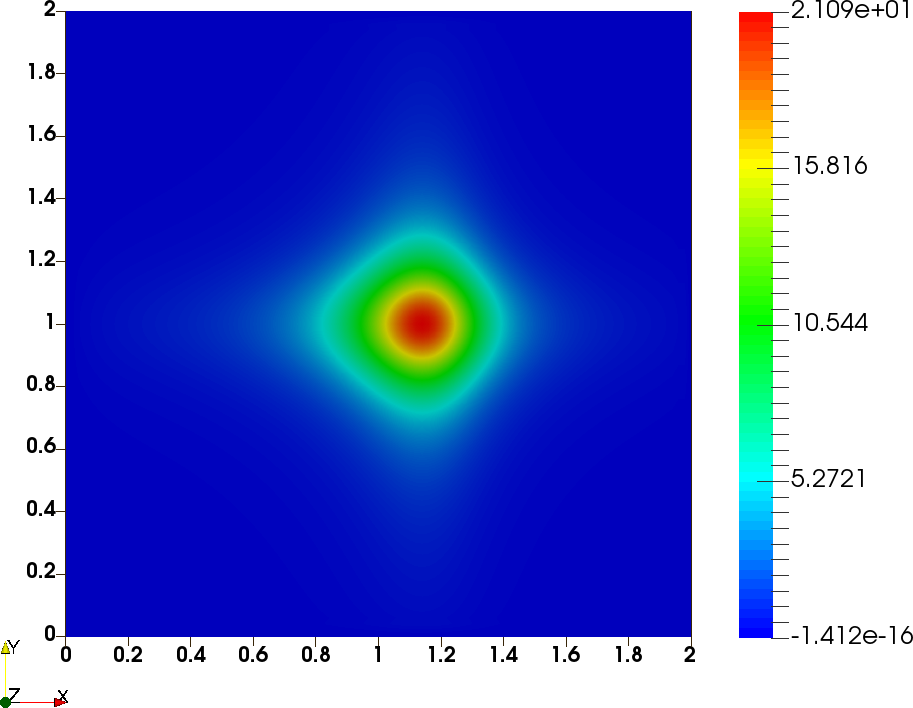
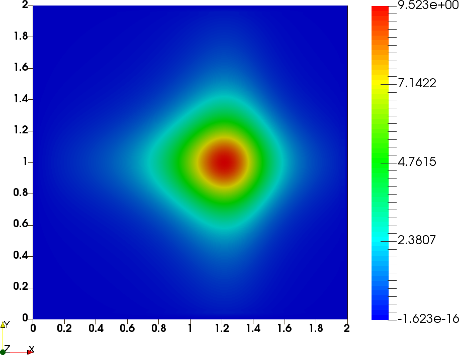
(a) Evolution of non-symmetric super-diffusive concentration field due to $p_{1}=0.35<0.5=p_{2}$ and$\boldsymbol{\alpha}=\boldsymbol{1.2}$ .

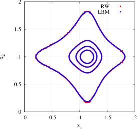
(b) Iso-levels $C=0.5,\,5,\,10,\,15$ at $t=0.6$ for RW (red) and LBM (blue).

Figure 4: Global views of the solutions to Eq. (1) equipped with the same parameters as for Fig.3, and showing (a) time evolution and (b) iso-levels issued of LBM and RW.

Validation 3: Three-dimensional simulations with LBM and RW

BGK LBM captures the anisotropic contours in perfect agreement with random walks in dimension three also. Fig. 5 documents the solutions of Eq. (1) in $\Omega=[0,\,1]^{3}$ for $\boldsymbol{\alpha}=\mathbf{1.2}$, $\boldsymbol{p}=(0.35,\,0.5,\,0.5)^{T}$ and $\overline{\overline{\mathbf{D}}}=0.5\overline{\overline{\mathbf{Id}}}$. The initial Gaussian hill is located near the center $\mathbf{x}^{s}=(0.5,\,0.5,\,0.5)^{T}$ of the cube. Similar trend is observed as in dimension two, except that the more confined geometry results into iso-contours (displayed on Fig. 5a) and iso-surfaces (displayed on Fig. 5b) showing smaller curvature. Global views and especially non-spherical iso-surface (see Fig. 5b) illustrate the anisotropy due to our choice of vector $\boldsymbol{p}$, already visible on the right panel of Fig. 5a. The profiles recorded on several lines in $\Omega$ and the contour levels recorded in several planes validate BGK LBM and random walks simulations. Here we present on Fig. 5a only one particular $x_{1}$-profile and contour levels in the particular $x_{1}x_{3}$-plane at $t=0.21$. These figures are issued from a computation using space and time steps $\Delta x=0.0125$ and $\Delta t=3\times 10^{-5}$, with $80^{3}$ nodes. It took 13.12h to perform $7\times 10^{3}$ time steps on a single core.

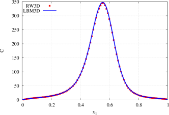
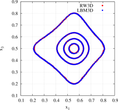
(a) Comparisons between solutions random walk (red) and LBM (blue) approximations to the 3D Eq. (1) for $\mathbf{u}=\mathbf{0}$: parameter $p_{1}<0.5$ (equivalent to $\beta_{1}<0$) shifts the maximum toward larger $x_{1}$. Left: $C(x_{1},\,x_{2}^{s},\,x_{3}^{s},\,t)$-profile at $t=0.21$. Right: iso-levels $C=15,\,100,\,200,\,300$ for $x_{2}=x_{2}^{s}$.

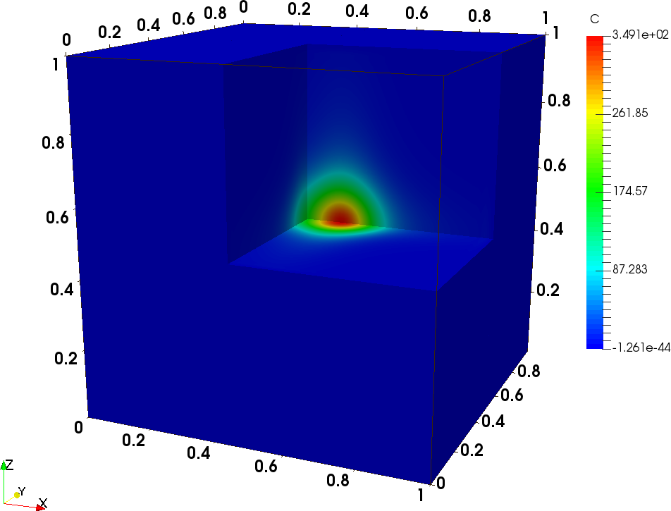
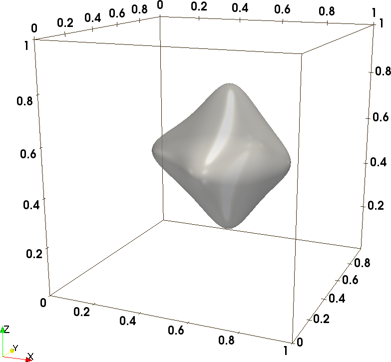
(b) Global concentration field at $t=0.21$ illustrated by color levels on section views of the three planes $x_{\mu}=0.5$ (left), and by perspective view of iso-surface $C=15$ (right).

Figure 5: Solutions to three-dimensional Eq. (1) in $\Omega=[0,\,1]^{3}$ with parameters $\boldsymbol{\alpha}=\boldsymbol{1.2}$, $\boldsymbol{g}=\boldsymbol{1}$ and $\boldsymbol{p}=(0.35,\,0.5,\,0.5)^{T}$ supplemented by $\mathbf{u}=\mathbf{0}$ and spherical $\overline{\overline{\mathbf{D}}}$. Above: LBM and random walk return indistinguishable $C(x_{1},\,x_{2}^{s},\,x_{3}^{s},\,t)$ profile (left) and iso-levels $C(x_{1},\,x_{2}^{s},\,x_{3},\,t)$ in $x_{1}x_{3}$-plane (right). Below: three-dimensional iso-surfaces.

These three tests validate the algorithm and the equilibrium distribution function described in Section 2 based on fractional integrals approximated at order two according to Section 2.4. Lower order approximations do not return so good agreement between LBM and RW.

3.3 Instabilities due to $\mathbf{u}\neq\mathbf{0}$ in the LBM

Numerical approximations to the classical ADE are often subjected to instabilities when Péclet numbers are increased. The additional freedom degrees included in MRT collision operator help us fixing such shortcoming better than BGK [26]. Fractional equations [23, 45] also are subjected to such instabilities.

Finite difference schemes approximating the one-dimensional ADE become unstable at large Péclet number, even in implicit versions. We also experience it on the LBM equipped with BGK collision operator adapted to the ADE with parameters with $D_{11}=D_{22}=2\times 10^{-3}$, $\boldsymbol{p}=\boldsymbol{1}/\mathbf{2}$ and $\mathbf{u}=(5,\,0)^{T}$ at times $t>0.128$. The domain is $\Omega=[0,\,2]\times[0,\,1]$, the initial condition described in 3.2 is centered at $(0.5,\,0.5)$, and the space- and time-steps are $\Delta x=10^{-2}$ and $\Delta t=8\times 10^{-4}$. Appropriately choosing $\lambda_{3}$ and $\lambda_{4}$ (e.g. $\lambda_{3}=\lambda_{4}>0.833$) in MRT setting re-stabilizes the LBM without sacrificing accuracy, as in [26].

The BGK LBM applied to Eq. (1) equipped with parameters $\boldsymbol{\alpha}=\mathbf{1.7}$, $\boldsymbol{p}=\mathbf{0.5}$, $\boldsymbol{g}=\mathbf{1}$ and with the above spherical tensor $\overline{\overline{\mathbf{D}}}$ needs $\lambda=0.548$ if the space-time mesh is as above. The BGK scheme is stable at $t=0.08$ (see Fig. 6a, cyan curve), but definitely unstable at $t=1$, at smaller velocity ($u_{1}=1$) than when we apply it to the ADE. Profiles and iso-levels represented on Figs 6a and 6b demonstrate that MRT LBM equipped with parameters $\lambda_{3}=\lambda_{4}=2.1277$ is stable at $t=1$, and in perfect agreement with random walk approximation. Stability and accuracy are still preserved by MRT LBM at velocity $u_{1}=1.3$ if we increase $\lambda_{3}=\lambda_{4}$ to $2.6316$. At larger velocity, several values of $\lambda_{3}$ and $\lambda_{4}$ are found to ensure the stability (even for $u_{1}=1.5$), but the LBM solution becomes less accurate. Nevertheless, the MRT collision achieves stability and accuracy (together) at velocities two times larger than the BGK which becomes poorly accurate at $u_{1}=0.7$ and does not preserve the symmetry of the concentration field.

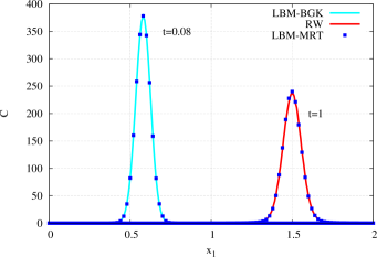
(a) $C(x_{1},\,0.5,\,t)$-profiles issued of BGK LBM (cyan), random walk (red) and MRT LBM (blue squares) at times $t=0.08$ and $t=1$: BGK is unstable for $t>0.08$, and not represented.

      

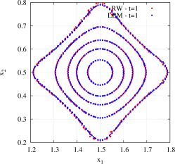
(b) Iso-levels $C=0.5,\,2.5,\,15,\,50,\,150$ issued of random walk (red dots) and MRT-LBM (blue squares) at $t=1$.

Figure 6: LBM and random walk approximations to Eq. (1) accounting for super-diffusion super-imposed to advection. The domain is $\Omega=[0,\,2]\times[0,\,1]$, the flow rate is $\mathbf{u}=u_{1}\mathbf{b}_{1}$ with $u_{1}=1$ and diffusion tensor is $\overline{\overline{\mathbf{D}}}=D\overline{\overline{\mathbf{Id}}}$ with $D=0.002$. Fractional parameters are $\boldsymbol{\alpha}=\mathbf{1.7}$, $\boldsymbol{g}=\mathbf{1}$ and $\boldsymbol{p}=\mathbf{0.5}$.

3.4 Validation of the LBM with exact solution

For certain boundary conditions and source term $S_{c}$, Eq. (1) admits exact solutions [23] that contribute to validate our numerical method if we allow $\overline{\overline{\mathbf{D}}}$ to depend on $\mathbf{x}$. Analytical solutions are derived from the relationship

$$\frac{\partial}{\partial x}I_{x+}^{1-\alpha^{\prime}}(x^{a})=\frac{\partial^{\alpha^{\prime}}x^{a}}{\partial_{+}x^{\alpha^{\prime}}}=x^{a-\alpha^{\prime}}\frac{\Gamma(a+1)}{\Gamma(a+1-\alpha^{\prime})}\quad\mbox{for}\quad a\geq\alpha^{\prime}\quad\mbox{and}\quad 1\geq\alpha^{\prime}$$ (26)

which is used with $\boldsymbol{p}=\mathbf{1}$ in simulations. In this case Eqs (1)-(2) become simpler because the second fractional integrals $I_{x_{\mu}-}^{2-\alpha_{\mu}}$ disappear. Assuming non-dimensional Eq. (1) equipped with $\mathbf{u}=\mathbf{0}$ and $\boldsymbol{g}=\boldsymbol{1}$ supplemented by a diagonal diffusion tensor $\overline{\overline{\mathbf{D}}}$ and a source term satisfying respectively

$$D_{\mu\mu}(\mathbf{x})=x_{\mu}^{\alpha_{\mu}}\frac{\Gamma(a_{\mu}+2-\alpha_{\mu})}{\Gamma(a_{\mu}+2)}\qquad\mbox{and}\qquad S_{c}(\mathbf{x},\,t)=-(d+1)e^{-t}\Pi_{\mu=1}^{d}x_{\mu}^{a_{\mu}},$$ (27)

we easily check that

$$C(\mathbf{x},\,t)=e^{-t}\Pi_{\mu=1}^{d}x_{\mu}^{a_{\mu}}$$ (28)

solves Eq. (1) in $\Omega=\Pi_{\mu=1}^{d}]0,\,L_{\mu}[$. Of course, we use initial data and boundary conditions dictated by Eq. (28).

The LBM scheme described by Algorithm 1 with the MRT collision operator retrieves these solutions of the two-dimensional Eq. (1), according to Fig. 7 where the stability parameters are $\alpha_{1}=1.5$, $\alpha_{2}=1.7$, with $a_{1}=0.4$ and $a_{2}=0.7$. In this case, time-dependent boundary condition and source term need being updated at each time step, and the time- and space-steps are $\Delta t=5\times 10^{-5}$ and $\Delta x=0.01$. Fig. 7 displays $C(x_{1},\,x_{2}^{s},\,t)$ and $C(x_{1}^{s},\,x_{2},\,t)$ profiles that demonstrate the good agreement between exact solution (solid and dash lines) and LBM simulation (symbols) at $t_{1}=0.05$, $t_{2}=0.5$ and $t_{3}=1$.

(a)	(b)

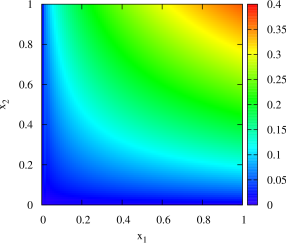
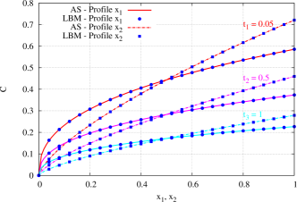
Figure 7: Solutions of the 2D Eq. (1) in the conditions described by Eqs (27). (a) Concentration field at $t=1$ from MRT LBM with $a_{1}=0.4$, $a_{2}=0.7$, $p_{1}=p_{2}=1$. (b) Comparisons of profiles between LBM and Analytical Solution (AS) $C(x_{1},\,x_{2},\,t)=e^{-t}x_{1}^{a_{1}}x_{2}^{a_{2}}$ for three times: $t_{1}=0.05$ (red), $t_{2}=0.5$ (magenta) and $t_{3}=1$ (cyan).

3.5 A variant of Eq. (2)

Eq. (2) specifies the entries of vector $\boldsymbol{\mathcal{F}}^{\boldsymbol{\alpha}\boldsymbol{p}\boldsymbol{g}}(C)$ that determines the dispersive flux $\overline{\overline{\mathbf{D}}}(\mathbf{x})\boldsymbol{\mathcal{F}}^{\boldsymbol{\alpha}\boldsymbol{p}\boldsymbol{g}}(C)$ in Eq. (1). When all its coefficients are independent of $\mathbf{x}$, Eq. (2) is equivalent to dispersive flux based on Riemann-Liouville derivatives as particle fluxes in random walks based on stable process [20]. This motivated our choice of the ordering of derivative and integral in Eq. (2), used in most applications of space-fractional diffusion equation. This choice returns an evolution equation (Eq. (6)) that preserves the positivity at least in the particular cases studied in [21]. However, it is sometimes questioned because it implies that Eq. (1) does not admit independent of $\mathbf{x}$ equilibria for $\boldsymbol{\alpha}\neq\boldsymbol{2}$. Replacing the Riemann-Liouville derivatives of the order of $\alpha_{\mu}$ in (6) by Caputo type derivatives of the form of $I_{x_{\mu}\pm}^{2-\alpha}\frac{\partial^{2}}{\partial x_{\mu}^{2}}$ would return an evolution equation admitting such equilibria but badly suited for mass transport studies because it does not preserve positivity [21]. However, the same reference points that replacing $\boldsymbol{\mathcal{F}}^{\boldsymbol{\alpha}\boldsymbol{p}\boldsymbol{g}}(C)$ by $\tilde{\boldsymbol{\mathcal{F}}}^{\boldsymbol{\alpha}\boldsymbol{p}\boldsymbol{g}}(C)$ defined by [39]

$$\tilde{\boldsymbol{\mathcal{F}}}^{\boldsymbol{\alpha}\boldsymbol{p}\boldsymbol{g}}(C)=\sum_{\mu=1}^{d}\tilde{\mathcal{F}}_{\mu}^{\alpha_{\mu}p_{\mu}g_{\mu}}(C)\mathbf{b}_{\mu},\quad\tilde{\mathcal{F}}_{\mu}^{\alpha_{\mu}p_{\mu}g_{\mu}}(C)=p_{\mu}I_{x_{\mu}+}^{2-\alpha_{\mu}}\frac{\partial}{\partial x_{\mu}}(g_{\mu}C)+(1-p_{\mu})I_{x_{\mu}-}^{2-\alpha_{\mu}}\frac{\partial}{\partial x_{\mu}}(g_{\mu}C)$$ (29)

inserts Caputo type derivatives into the dispersive flux [39, 46]. This results into a variant of Eq. (6) that preserves positivity (in the particular cases considered in [21]), and of course admits uniform equilibria. Though we do not know experimental data to which the variant was applied, adapting to it the LBM scheme presented in Section 2 just needs slightly modified equilibrium function.

Indeed, $\boldsymbol{\mathcal{F}}^{\boldsymbol{\alpha}\boldsymbol{p}\boldsymbol{g}}(C)$ and $\tilde{\boldsymbol{\mathcal{F}}}^{\boldsymbol{\alpha}\boldsymbol{p}\boldsymbol{g}}(C)$ only differ by a quantity related to the values of $C$ on the boundary $\partial\Omega$ of $\Omega$, because in the dimension $1$ with $\Omega=]\ell,\,L[$ integration by parts yields

$$(I_{x+}^{2-\alpha}\frac{\partial}{\partial x}f)(x)=\frac{\partial}{\partial x}\left[I_{x+}^{2-\alpha}f(x)-f(\ell)\frac{(x-\ell)^{2-\alpha}}{\Gamma(3-\alpha)}\right],\qquad(I_{x-}^{2-\alpha}\frac{\partial}{\partial x}f)(x)=\frac{\partial}{\partial x}\left[I_{x-}^{2-\alpha}f(x)-f(L)\frac{(L-x)^{2-\alpha}}{\Gamma(3-\alpha)}\right].$$ (30)

In higher dimension $d$ we apply this formula to the left/right fractional integrals w.r.t. the $x_{\mu}$ in Eqs. (3). The integration intervals are $\omega_{\pm}(\mathbf{x},\,\mu)$, and the link between $\boldsymbol{\mathcal{F}}^{\boldsymbol{\alpha}\boldsymbol{p}\boldsymbol{g}}(C)(\mathbf{x})$ and $\tilde{\boldsymbol{\mathcal{F}}}^{\boldsymbol{\alpha}\boldsymbol{p}\boldsymbol{g}}(C)(\mathbf{x})$ depends on the values taken by $C$ at the bounds of the $\omega_{\pm}(\mathbf{x},\,\mu)$ that stay on $\partial\Omega$. They correspond to $\ell$ or $L$ in (30) depending on whether we have $+$ or $-$ in $\pm$. For general domain $\Omega$ we call these points $\partial\omega_{\pm}(\mathbf{x},\,\mu)$, and their coordinates $z_{\pm\nu}(\mathbf{x},\,\mu)$: the latter coincide with the $x_{\nu}$ for $\nu\neq\mu$. For $\nu=\mu$ they are the lower and the upper bound of the projection on $\mathbf{b}_{\mu}$ of $\omega_{+}(\mathbf{x},\,\mu)$ and $\omega_{-}(\mathbf{x},\,\mu)$ (the other bound of the interval is $x_{\mu}$). In the domain $\Omega=\Pi_{\mu=1}^{d}]\ell_{\mu},\,L_{\mu}[$ which we use for our comparisons $z_{+\nu}(\mathbf{x},\,\mu)=\ell_{\mu}$ and $z_{-\nu}(\mathbf{x},\,\mu)=L_{\mu}$. With these notations, for general $\Omega$ we have

$$(I_{x_{\mu}+}^{2-\alpha_{\mu}}\frac{\partial}{\partial x_{\mu}}C)(\mathbf{x},t) =\frac{\partial}{\partial x_{\mu}}\left[I_{x_{\mu}+}^{2-\alpha_{\mu}}C(\mathbf{x},t)-C(\partial\omega_{+}(\mathbf{x},\,\mu),\,t)\frac{(x_{\mu}-z_{+\mu})^{2-\alpha_{\mu}}}{\Gamma(3-\alpha_{\mu})}\right],$$ (31a)

$$(I_{x_{\mu}-}^{2-\alpha_{\mu}}\frac{\partial}{\partial x_{\mu}}C)(\mathbf{x},t) =\frac{\partial}{\partial x_{\mu}}\left[I_{x_{\mu}-}^{2-\alpha_{\mu}}C(\mathbf{x},t)-C(\partial\omega_{-}(\mathbf{x},\,\mu),\,t)\frac{(z_{-\mu}-x_{\mu})^{2-\alpha_{\mu}}}{\Gamma(3-\alpha_{\mu})}\right].$$ (31b)

This implies

$$\tilde{\mathcal{F}}_{\mu}^{\alpha_{\mu}p_{\mu}g_{\mu}}C(\mathbf{x},t) =\frac{\partial}{\partial x_{\mu}}\left[p_{\mu}\left\{I_{x_{\mu}+}^{2-\alpha_{\mu}}(g_{\mu}C)(\mathbf{x},t)-g_{\mu}C(\partial\omega_{+}(\mathbf{x},\,\mu),\,t)\frac{(x_{\mu}-z_{+\mu})^{2-\alpha_{\mu}}}{\Gamma(3-\alpha_{\mu})}\right\}+\right.$$

$$\qquad\qquad\qquad\qquad\left.(1-p_{\mu})\left\{I_{x_{\mu}-}^{2-\alpha_{\mu}}(g_{\mu}C)(\mathbf{x},t)-g_{\mu}C(\partial\omega_{-}(\mathbf{x},\,\mu),\,t)\frac{(z_{-\mu}-x_{\mu})^{2-\alpha_{\mu}}}{\Gamma(3-\alpha_{\mu})}\right\}\right],$$ (32)

which suggests an equilibrium function defined by Eq. (13a) with

$$\mathcal{A}_{i}(\mathbf{x},\,t)=\begin{cases}C(\mathbf{x},\,t)-w_{0}\sum_{\mu=1}^{d}\left[p_{\mu}\left\{I_{x_{\mu}+}^{2-\alpha_{\mu}}g_{\mu}C(\mathbf{x},t)-g_{\mu}C\left(\partial\omega_{+}(\mathbf{x},\,\mu),\,t\right)\frac{(x_{\mu}-z_{+\mu})^{2-\alpha_{\mu}}}{\Gamma(3-\alpha_{\mu})}\right\}+\right.\\ \qquad\qquad\qquad\qquad\qquad\left.(1-p_{\mu})\left\{I_{x_{\mu}-}^{2-\alpha_{\mu}}g_{\mu}C(\mathbf{x},t)-g_{\mu}C\left(\partial\omega_{-}(\mathbf{x},\,\mu),\,t\right)\frac{(z_{-\mu}-x_{\mu})^{2-\alpha_{\mu}}}{\Gamma(3-\alpha_{\mu})}\right\}\right]&\mbox{if}\,\,i=0\\ \\ w_{i}\left[p_{\mu}\left\{I_{x_{\mu}+}^{2-\alpha_{\mu}}g_{\mu}C(\mathbf{x},t)-g_{\mu}C\left(\partial\omega_{+}(\mathbf{x},\,\mu),\,t\right)\frac{(x_{\mu}-z_{+\mu})^{2-\alpha_{\mu}}}{\Gamma(3-\alpha_{\mu})}\right\}+\right.\\ \qquad\qquad\qquad\qquad\qquad\left.(1-p_{\mu})\left\{I_{x_{\mu}-}^{2-\alpha_{\mu}}g_{\mu}C(\mathbf{x},t)-g_{\mu}C\left(\partial\omega_{-}(\mathbf{x},\,\mu),\,t\right)\frac{(z_{-\mu}-x_{\mu})^{2-\alpha_{\mu}}}{\Gamma(3-\alpha_{\mu})}\right\}\right]&\mbox{if}\,\,i\neq 0\end{cases}$$ (33)

instead of (13b). We check this equilibrium function in two dimensions by setting $\ell_{\mu}=0$, $L_{\mu}=1$, $D_{\mu}=1$, $g_{\mu}=1$ for $\mu=1,\,2$ and noting that $C(\mathbf{x},\,t)=e^{-t}\Pi_{\mu=1}^{2}(x_{\mu}^{\alpha_{\mu}}+a_{\mu})$ satisfies Eq. (1) equipped with $\tilde{\boldsymbol{\mathcal{F}}}^{\boldsymbol{\alpha}\boldsymbol{p}\boldsymbol{g}}(C)$ instead of $\boldsymbol{\mathcal{F}}^{\boldsymbol{\alpha}\boldsymbol{p}\boldsymbol{g}}(C)$ provided we also set $\mathbf{u}=\mathbf{0}$, $p_{\mu}=1$ for $\mu=1,\,2$, and

$$S_{c}(\mathbf{x},\,t)=-e^{-t}\left[\Pi_{\mu=1}^{2}(x_{\mu}^{\alpha_{\mu}}+a_{\mu})+D_{1}\Gamma(\alpha_{1}+1)(x_{2}^{\alpha_{2}}+a_{2})+D_{2}\Gamma(\alpha_{2}+1)(x_{1}^{\alpha_{1}}+a_{1})\right].$$ (34)

With the modified equilibrium distribution function, the LBM of Section 2 equipped with the equilibrium function defined by (33) retrieves the exact solution if we apply Dirichlet boundary conditions (resp. initial condition) dictated by $C(\mathbf{x},\,t)=e^{-t}\Pi_{\mu=1}^{2}(x_{\mu}^{\alpha_{\mu}}+a_{\mu})$ (for $a_{\mu}\neq 0$) on the boundaries of $\Omega$ (resp. at $t=0$). A look at the figures 8(a),(b) checks this fact. For comparisons of Figs. 8 (a), (b), we choose fractional parameters $\alpha_{1}=1.7$, $\alpha_{2}=1.2$, $a_{1}=0.3$, $a_{2}=1.2$ and $p_{1}=p_{2}=1$. The other numerical parameters for LBM are $\Delta x=0.02$, $\Delta t=2.5\times 10^{-5}$, $N_{x_{1}}=N_{x_{2}}=101$. Comparisons between LBM (symbols) and analytical solution (solid lines) are presented for two times $t_{1}=0.025$ and $t_{2}=0.425$ along $x_{1}$- and $x_{2}$-profiles respectively for $x_{2}=1$ and $x_{1}=1$.

(a)		(b)

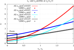
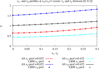
Figure 8: Comparison between LBM and Analytical Solution (AS) for Eq. (1) equipped with $\tilde{\boldsymbol{\mathcal{F}}}^{\boldsymbol{\alpha}\boldsymbol{p}\boldsymbol{g}}(C)$ defined by Eq. (32) instead of $\mathcal{F}_{\mu}^{\alpha_{\mu}p_{\mu}g_{\mu}}C(\mathbf{x},\,t)$.

4 Conclusion

We discussed Lattice Boltzmann schemes that simulate $d$-dimensional fractional equation (Eq. (1)) for $d=2$ or $3$. In this conservation equation, the solute flux splits into classical advective part and dispersive contribution accounting for super-diffusion. The latter is obtained by applying a regular diffusivity tensor to a $d$-dimensional vector whose entry of rank $\mu$ is the partial derivative w.r.t. $x_{\mu}$ of a linear combination of two fractional integrals w.r.t. this coordinate. Moreover, the LBM splits the concentration into $\mathcal{N}+1$ populations whose velocities belong to a lattice (here D2Q5 for $d=2$ and D3Q7 for $d=3$), and uses $\mathcal{N}+1$ equilibrium distributions for these populations. The above mentioned fractional integrals provide us equilibrium distributions which cause that the total concentration approximately solves Eq. (1). The complementarity of the equilibrium function with BGK or MRT collision rules returns accurate numerical solutions provided the fractional integrals are discretized with precision.

Eq. (1) with Dirichlet boundary conditions has exact solutions and random walk approximations valid when its parameters satisfy incompatible conditions. Exact solutions hold for $\boldsymbol{p}=\boldsymbol{0}$ or $\boldsymbol{1}$ supplemented by specific space dependent coefficients. Random walk approximations are more generic. They may be flawed by noise (if we do not use sufficiently many walkers) but not by numerical diffusion or instability. Comparisons with random walks and exact solutions revealed that MRT collision rule approximates the solutions of Eq. (1) as accurately as BGK collision rule, even near the boundaries. Yet, the BGK rule does not adapt to all anisotropic diffusion tensor and returns solutions that become unstable at moderately large advection speed. Compared with the ADE, space fractional diffusion equations are more sensitive to such numerical instabilities. MRT LBM is accurate in more general conditions, and less unstable because it includes additional freedom degrees whose values can be chosen so as to damp perturbations.

The LBM scheme approximates Eq. (1) associated to dispersive flux based on Riemann-Liouville or Caputo derivatives as well provided we choose appropriate equilibrium function.

Random walks and LBM can be viewed as complementary methods that approximate the solutions of p.d.es as Eq. (1) and check each other accuracy. The latter depends of their time steps (independent of each other), which of course influence the computing times which are different. According to our comparisons (not using parallel computing) the LBM is four times more rapid in the dimension 3, except when we can use the independence of the coordinates of $\mathbf{X}^{\Omega}(t)$ (with spatially homogeneous parameters when domain $\Omega$ is a rectangle). In this case the random walk is ten times more rapid because it relies upon one-dimensional simulations. In the dimension $d=2$ its computing time is similar to that of the LBM if we do not use the independence property. Hence, the LBM will be preferred in the dimension three in general domain or with spatially heterogeneous parameters, and will become especially useful in tasks that accumulate many successive simulations. Nevertheless, the LBM needs being assessed by point-wise comparisons with random walk.

Appendix A Asymptotic analysis of the LBE associated with the equilibrium function adapted to the fractional ADE

With the equilibrium function defined by Eqs. (13a)-(13b), the LBE approximates the solutions of Eq. (1) if $\boldsymbol{\alpha}=\boldsymbol{2}$, within BGK as well as MRT setting. Allowing $\boldsymbol{\alpha}<\boldsymbol{2}$ only requires to modify the final steps of the classical Chapman-Enskog expansion. The reasoning is based on the Taylor expansion of $\mathbb{T}\bigr{|}\boldsymbol{f}\bigr{\rangle}$ (defined by Eq. (9b)) combined with Eq. (10) and the expansion $\bigr{|}\boldsymbol{f}\bigr{\rangle}=\sum_{k\geq 0}\varepsilon^{k}\bigr{|}\boldsymbol{f}^{(k)}\bigr{\rangle}$. Moreover it assumes bounded derivatives w.r.t $t_{1}$, $t_{2}$ and $x^{\prime}_{1}$, …, $x^{\prime}_{d}$ for $\bigr{|}\boldsymbol{f}^{(k)}\bigr{\rangle}$. We recall for convenience the method that sequentially collects the items of each order $\varepsilon^{k}$, and yields a sequence of equations satisfied by the first moments of the $\bigr{|}\boldsymbol{f}^{(k)}\bigr{\rangle}$, especially $\langle\mathbf{1}|\boldsymbol{f}^{(0)}\rangle=C$. More specifically, we show that Eqs. (11) and (12a)-(12c) imply that $\langle\mathbf{1}|\boldsymbol{f}^{(0)}\rangle$ is solution of Eq. (1) within an error of $O(\varepsilon^{2})$.

Order $\varepsilon^{0}$ writes $0=\mathbf{M}^{-1}\boldsymbol{\Lambda}\mathbf{M}\left[\bigr{|}\boldsymbol{f}^{eq}\bigr{\rangle}-\bigr{|}\boldsymbol{f}^{(0)}\bigr{\rangle}\right]$ and implies

$$\bigr{|}\boldsymbol{f}^{(0)}\bigr{\rangle}=\bigr{|}\boldsymbol{f}^{eq}\bigr{\rangle}$$ (35)

because $\mathbf{M}^{-1}\boldsymbol{\Lambda}\mathbf{M}$ is invertible with BGK or MRT matrices $\mathbf{M}$ and $\boldsymbol{\Lambda}$. Collisions preserving the total solute mass imply Eq. (12a), hence

$$\langle\mathbf{1}\bigr{|}\boldsymbol{f}^{(k)}\bigr{\rangle}=0\quad\mathrm{for}\quad k>0.$$ (36)

If we assume $S_{c}=S\varepsilon^{2}$ for the source rate, orders $\varepsilon$ and $\varepsilon^{2}$ yield respectively

$$\Delta t\frac{\partial}{\partial t_{1}}\bigr{|}\boldsymbol{f}^{(0)}\bigr{\rangle}+\Delta x\frac{\partial}{\partial x_{\mu}^{\prime}}\bigr{|}e_{\mu}\boldsymbol{f}^{(0)}\bigr{\rangle}=-\mathbf{M}^{-1}\boldsymbol{\Lambda}\mathbf{M}\bigr{|}\boldsymbol{f}^{(1)}\bigr{\rangle}$$ (37)

and

$$\Delta t\left[\frac{\partial}{\partial t_{1}}\bigr{|}\boldsymbol{f}^{(1)}\bigr{\rangle}+\frac{\partial}{\partial t_{2}}\bigr{|}\boldsymbol{f}^{(0)}\bigr{\rangle}\right]+\Delta x\frac{\partial}{\partial x^{\prime}_{\mu}}\bigr{|}e_{\mu}\boldsymbol{f}^{(1)}\bigr{\rangle}+\frac{\Delta t^{2}}{2}\frac{\partial^{2}}{\partial t_{1}^{2}}\bigr{|}\boldsymbol{f}^{(0)}\bigr{\rangle}\qquad$$

$$+\Delta t\Delta x\frac{\partial^{2}}{\partial t_{1}\partial x^{\prime}_{\mu}}\bigr{|}e_{\mu}\boldsymbol{f}^{(0)}\bigr{\rangle}+\frac{\Delta x^{2}}{2}\frac{\partial^{2}}{\partial x^{\prime}_{\mu}\partial x^{\prime}_{\nu}}\bigr{|}e_{\mu}e_{\nu}\boldsymbol{f}^{(0)}\bigr{\rangle} =-\mathbf{M}^{-1}\boldsymbol{\Lambda}\mathbf{M}\bigr{|}\boldsymbol{f}^{(2)}\bigr{\rangle}+\Delta tS\left|\mathbf{w}\right\rangle$$ (38)

in which $a_{\mu}b_{\mu}$ and $\partial b_{\mu}/\partial a_{\mu}$ represent $\sum_{\mu=1}^{d}a_{\mu}b_{\mu}$ and $\sum_{\mu=1}^{d}\partial b_{\mu}/\partial a_{\mu}$ respectively.

Eq. (37) is equivalent to

$$-\mathbf{M}\bigr{|}\boldsymbol{f}^{(1)}\bigr{\rangle}=\boldsymbol{\Lambda}^{-1}\mathbf{M}\left[\Delta t\frac{\partial}{\partial t_{1}}\bigr{|}\boldsymbol{f}^{(0)}\bigr{\rangle}+\Delta x\frac{\partial}{\partial x^{\prime}_{\mu}}\bigr{|}e_{\mu}\boldsymbol{f}^{(0)}\bigr{\rangle}\right].$$ (39)

which determines $\bigr{|}\boldsymbol{f}^{(1)}\bigr{\rangle}$ and implies (projection on $\bigr{|}\boldsymbol{1}\bigr{\rangle}$)

$$\Delta t\frac{\partial}{\partial t_{1}}\langle\mathbf{1}|\boldsymbol{f}^{(0)}\rangle+\Delta x\frac{\partial}{\partial x^{\prime}_{\mu}}\langle e_{\mu}|\boldsymbol{f}^{(0)}\rangle=0$$ (40)

in view of (36). Summing up $\varepsilon$ times (40) and $\varepsilon^{2}$ times the projection of (38) on $\bigr{|}\boldsymbol{1}\bigr{\rangle}$ yields

$$\Delta t\left[\varepsilon\frac{\partial}{\partial t_{1}}+\varepsilon^{2}\frac{\partial}{\partial t_{2}}\right]\bigr{\langle}\boldsymbol{1}|\boldsymbol{f}^{(0)}\bigr{\rangle}+\Delta x\varepsilon\frac{\partial}{\partial x^{\prime}_{\mu}}\bigr{\langle}e_{\mu}|\boldsymbol{f}^{(0)}\bigr{\rangle}+\Delta x\varepsilon^{2}\frac{\partial}{\partial x^{\prime}_{\mu}}\bigr{\langle}e_{\mu}|\boldsymbol{f}^{(1)}\bigr{\rangle}\qquad$$

$$+\frac{\Delta x\Delta t}{2}\varepsilon^{2}\frac{\partial^{2}}{\partial x^{\prime}_{\mu}\partial t_{1}}\bigr{\langle}e_{\mu}|\boldsymbol{f}^{(0)}\bigr{\rangle}+\frac{\Delta x^{2}}{2}\varepsilon^{2}\frac{\partial^{2}}{\partial x^{\prime}_{\mu}\partial x^{\prime}_{\nu}}\bigr{\langle}e_{\mu}|e_{\nu}\boldsymbol{f}^{(0)}\bigr{\rangle} =\Delta t\varepsilon^{2}S\bigr{|}\mathbf{w}\bigr{\rangle}$$ (41)

in which the two first items are $\Delta t\partial_{t}\bigr{\langle}\boldsymbol{1}|\boldsymbol{f}^{(0)}\bigr{\rangle}$ and $\Delta t\boldsymbol{\nabla}\cdot\mathbf{u}C$ (in view of Eqs. (10) and (12b)) with an error of the order of $\varepsilon^{2}$. Then, Eq. (37) implies more or less simple expression for $|\boldsymbol{f}^{(1)}\bigr{\rangle}$ in BGK or MRT setting.

A.1 BGK

The BGK collision operator assumes $\mathbf{M}=\mathbf{I}$ and $\boldsymbol{\Lambda}^{-1}=\lambda\mathbf{I}$, so that Eq. (37) implies

$$-\bigr{|}\boldsymbol{f}^{(1)}\bigr{\rangle}=\lambda\left[\Delta t\frac{\partial}{\partial t_{1}}|\boldsymbol{f}^{(0)}\rangle+\Delta x\frac{\partial}{\partial x^{\prime}_{\mu}}\bigr{|}e_{\mu}\boldsymbol{f}^{(0)}\bigr{\rangle}\right].$$ (42)

hence

$$-\bigl{\langle}e_{\nu}\bigr{|}\boldsymbol{f}^{(1)}\bigr{\rangle}=\lambda\left[\Delta t\frac{\partial}{\partial t_{1}}\bigl{\langle}e_{\nu}\bigr{|}\boldsymbol{f}^{(0)}\bigr{\rangle}+\Delta x\frac{\partial}{\partial x^{\prime}_{\mu}}\bigl{\langle}e_{\nu}e_{\mu}\bigr{|}\boldsymbol{f}^{(0)}\bigr{\rangle}\right].$$ (43)

Combining the latter with Eqs (10) and (41) yields

$$\Delta t\frac{\partial}{\partial t}\bigl{\langle}\mathbf{1}\bigr{|}\boldsymbol{f}^{(0)}\bigr{\rangle}+\Delta x\frac{\partial}{\partial x_{\mu}}\bigl{\langle}e_{\mu}\bigr{|}\boldsymbol{f}^{(0)}\bigr{\rangle}-\left(\lambda-\frac{1}{2}\right)\Delta x\Delta t\frac{\partial^{2}}{\partial t\partial x_{\mu}}\bigl{\langle}e_{\mu}\bigr{|}\boldsymbol{f}^{(0)}\bigr{\rangle}-\left(\lambda-\frac{1}{2}\right)\Delta x^{2}\frac{\partial^{2}}{\partial x_{\mu}\partial x_{\nu}}\bigl{\langle}e_{\mu}e_{\nu}\bigr{|}\boldsymbol{f}^{(0)}\bigr{\rangle}=S_{c}\Delta t.$$ (44)

Neglecting the third term $(\lambda-1/2)\Delta x\Delta t\partial_{tx_{\mu}}^{2}\bigl{\langle}e_{\mu}\bigr{|}\boldsymbol{f}^{(0)}\bigr{\rangle}$ and using Eq. (12c) yields Eq. (1) provided $\overline{\overline{\mathbf{D}}}=D\overline{\overline{\mathbf{Id}}}$ if, moreover, Eq. (11) is satisfied.

A.2 MRT

With MRT matrices $\mathbf{M}$ and $\boldsymbol{\Lambda}^{-1}$, Eq. (39) implies

$$-\langle e_{\nu}|\boldsymbol{f}^{(1)}\rangle=\lambda_{\nu\rho}\left[\Delta t\frac{\partial}{\partial t_{1}}\langle e_{\rho}|\boldsymbol{f}^{(0)}\rangle+\Delta x\frac{\partial}{\partial x^{\prime}_{\mu}}\langle e_{\rho}e_{\mu}|\boldsymbol{f}^{(0)}\rangle\right],$$ (45)

very similar to Eq. (43) if we set $\overline{\overline{\boldsymbol{\lambda}}}$ for the $d\times d$ matrix of entries $\lambda_{\mu\nu}$. Recalling Eqs (36) and (10) in Eq. (41) yields

$$\Delta t\left[\frac{\partial}{\partial t}\bigl{\langle}\mathbf{1}\bigr{|}\boldsymbol{f}^{(0)}\bigr{\rangle}+\nabla\cdot(C\boldsymbol{u})\right]+\Delta t\Delta x\left(-\frac{\partial}{\partial t}\lambda_{\mu\rho}\frac{\partial}{\partial x_{\rho}}\bigl{\langle}e_{\rho}\bigr{|}\boldsymbol{f}^{(0)}\bigr{\rangle}+\frac{1}{2}\frac{\partial^{2}}{\partial t\partial x_{\mu}}\bigl{\langle}e_{\rho}\bigr{|}\boldsymbol{f}^{(0)}\bigr{\rangle}\right)\qquad\qquad\qquad$$ (46)

$$+\Delta x^{2}\left[\frac{1}{2}\frac{\partial^{2}}{\partial x_{\mu}\partial x_{\nu}}\bigl{\langle}e_{\mu}e_{\nu}\bigr{|}\boldsymbol{f}^{(0)}\bigr{\rangle}-\frac{\partial}{\partial x_{\mu}}\lambda_{\mu\rho}\frac{\partial}{\partial x_{\nu}}\bigl{\langle}e_{\rho}e_{\nu}\bigr{|}\boldsymbol{f}^{(0)}\bigr{\rangle}\right] =S_{c}\Delta t,$$ (47)

in view of $\bigl{\langle}e_{\mu}\bigr{|}\boldsymbol{f}^{(0)}\bigr{\rangle}=u_{\mu}C\Delta t/\Delta x$ (i.e. (12b)). Using Eq. (12c), $\bigl{\langle}e_{\rho}e_{\nu}\bigr{|}\boldsymbol{f}^{(0)}\bigr{\rangle}=\delta_{\rho\nu}[p_{\nu}I_{x_{\nu}+}^{2-\alpha_{\nu}}(g_{\nu}C)+(1-p_{\nu})I_{x_{\nu}-}^{2-\alpha_{\nu}}(g_{\nu}C)]$ and neglecting the second term $\Delta t\Delta x(-\partial_{t}\lambda_{\mu\rho}\partial_{x_{\rho}}\bigl{\langle}e_{\rho}\bigr{|}\boldsymbol{f}^{(0)}\bigr{\rangle}+\partial_{tx_{\mu}}^{2}\bigl{\langle}e_{\rho}\bigr{|}\boldsymbol{f}^{(0)}\bigr{\rangle}/2)$ as above, we recognize Eq. (1) if $\overline{\overline{\boldsymbol{\lambda}}}$ satisfies Eq. (17) which we copy below for convenience

$$\overline{\mathbf{\overline{D}}}=e^{2}\left(\overline{\overline{\boldsymbol{\lambda}}}-\frac{1}{2}\overline{\overline{\mathbf{Id}}}\right)\frac{\Delta x^{2}}{\Delta t}.$$ (48)

The matrix $\overline{\overline{\boldsymbol{\lambda}}}$ may depend on $\mathbf{x}$ to account for spatially non-uniform tensor $\overline{\overline{\mathbf{D}}}$.

Appendix B Stable process and fractional equation

B.1 Stable Lévy laws

A look at the characteristic function

$$\langle e^{jkS(\alpha,\,\beta)}\rangle =e^{-\varphi_{\alpha,\,\beta}}(k)$$ (49)

$$\varphi_{\alpha,\,\beta}(k) =|k|^{\alpha}\left(1-j\beta\textrm{sign}(k)\tan\frac{\pi\alpha}{2}\right)$$ (50)

gives an idea of the role played by its two parameters: $\beta$ which ranges between $-1$ and $+1$ describes the degree of skewness of $\varphi_{\alpha,\,\beta}$ and the distribution of $S(\alpha,\,-\beta)$ is the mirror image of $S(\alpha,\,\beta)$. We also see that the influence of $\beta$ vanishes when $\alpha$ approaches $2$, a special value at which $S(\alpha,\,\beta)$ is standard centered Gaussian. The stability index $\alpha\in]0,\,2]$ describes the asymptotic decrease of the density $\mathbb{P}^{\alpha,\beta}(x)$, proportional to $x^{-\alpha-1}$ when $|x|\to\infty$ except for $\alpha=2$ and $x<0$ if $\beta=\pm 1$: decreasing $\alpha$ makes large values more probable and thickens the tails of the distribution of $S(\alpha,\,\beta)$ illustrated by Fig. 9. Large positive values of $\beta$ re-inforce the positive tail without changing the exponent of the asymptotic behavior, except if $\beta=1$, a special case in which the negative tail tapers off exponentially. The figure also shows that the most probable value of $S(\alpha,\,\beta)$ has the sign of $-\beta$ while Eqs (49)-(50) show that the average is always zero.

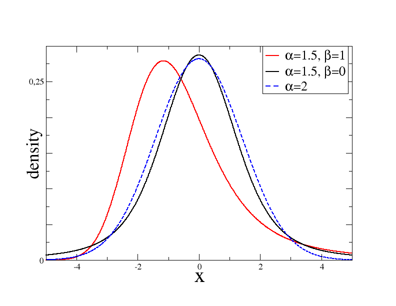
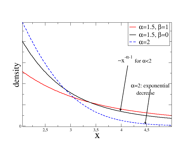
Figure 9: Lévy variable densities $\mathbb{P}^{\alpha,\beta}(x)$. Represented densities correspond to $\alpha=2$ (dashed blue line) and $\alpha=1.5$. The latter case is represented for two values of $\beta$: the solid black line represents the symmetric case $\beta=0$ and the solid red line represents $\beta=1$. Right panel shows a magnification of the asymptotic behavior of the densities at large positive values.

B.2 Stochastic process and fractional equation in bounded domain

That killed process p.d.fs satisfy Eq. (1) can be proved for rectangular domain $\Omega$ if the coefficients do not depend on $\mathbf{x}$. Indeed, reference [40] implies this result for one-dimensional symmetric process provided $\mathbf{u}=\mathbf{0}$, moreover assuming smooth initial condition compactly supported in $\Omega$. We easily extend it to higher dimension in $\Omega=\Pi_{\mu=1}^{d}]\ell_{\mu},\,L_{\mu}[$ for possibly non-symmetric process whose projections on the $\mathbf{b}_{\mu}$ are independent, as here. Indeed, the recent paper [43] states the result for general stable process and initial data provided $\Omega$ is regular in the sense of Probability (not of numerical analysis). However, one-dimensional intervals are regular. Moreover in our case the components of $\mathbf{X}(t)$ are mutually independent, and this extends to $\mathbf{X}^{\Omega}(t)$ when $\Omega$ is a rectangle of $\mathbb{R}^{d}$. Consequently, the density of $\mathbf{X}^{\Omega}(t)$ is of the form of $P=\Pi_{\mu=1}^{d}P_{\mu}(x_{\mu},\,t)$ where each one-dimensional density $P_{\mu}(x_{\mu},\,t)$ satisfies a one-dimensional version of Eq. (1). Hence $P$ satisfies the $d$-dimensional version. This proves that histograms of samples of $\mathbf{X}^{\Omega}(t)$ approximate solutions of Eq. (6) satisfying homogeneous Dirichlet conditions at the boundary of $\Omega$.

Validations 1 and 2 in Section 3.2 illustrate this result, predicted by [42]. Other boundary conditions were proved to achieve the equivalence of processes deduced from $\mathbf{X}$ and Eq. (1) in the case of spatially homogeneous parameters [21, 44], but there also exists boundary constraints whose application to $\mathbf{X}(t)$ severely modifies the equation that rules the p.d.f [45, 47].

References

- [1] D. Clarke, M. Meerschaert, S. Wheatcraft, Fractal travel time estimates for dispersive contaminants, Ground Water 43 (3) (2005) pp. 401–407.
- [2] S. Wheatcraft, S. Tyler, An explanation of scale-dependent dispersivity in heterogeneous aquifers using concepts of fractal geometry, Water Resources Research 24 (4) (1988) 566–578. doi:10.1029/WR024i004p00566.
- [3] R. Metzler, J. Klafter, The restaurant at the end of the random walk: recent developments in the description of anomalous transport by fractional dynamics, Journal of Physics A: Mathematical and General 37 (31) (2004) R161.
- [4] J. Clark, M. Silman, R. Kern, E. Macklin, J. HilleRisLambers, Seed dispersal near and far: Patterns across temperate and tropical forests, Ecology 80 (5) (1999) 1475–1494. doi:10.1890/0012-9658(1999)080[1475:SDNAFP]2.0.CO;2.
- [5] S. Fedotov, A. Iomin, Migration and proliferation dichotomy in tumor-cell invasion, Phys. Rev. Lett. 98 (2007) 118101. doi:10.1103/PhysRevLett.98.118101.
- [6] D. Benson, R. Schumer, M. Meerschaert, S. Wheatcraft, Fractional dispersion, lévy motion, and the made tracer tests, Transport in Porous Media 42 (1) (2001) 211–240. doi:10.1023/A:1006733002131.
- [7] Z.-Q. Deng, V. Singh, L. Bengtsson, Numerical solution of fractional advection-dispersion equation, Journal of Hydraulic Engineering 130 (5) (2004) 422–431.
- [8] D. Benson, S. Wheatcraft, M. Meerschaert, The fractional-order governing equation of lévy motion, Water Resources Research 36 (6) (2000) 1413–1423. doi:10.1029/2000WR900032.
- [9] R. Schumer, D. Benson, M. Meerschaert, S. Wheatcraft, Eulerian derivation of the fractional advection–dispersion equation, Journal of Contaminant Hydrology 48 (1–2) (2001) 69 – 88. doi:http://dx.doi.org/10.1016/S0169-7722(00)00170-4.
- [10] J. Kelly, D. Bolster, M. Meerschaert, J. Drummond, A. Packmann, Fracfit: A robust parameter estimation tool for fractional calculus models, Water Resources Research 53 (2016WR019748) (2017) 2559–2567, doi:10.1002/20016WR019748.
- [11] S. Samko, A. . Kilbas, O. Marichev, Fractional integrals and derivatives: theory and applications, Gordon and Breach, New York, 1993.
- [12] Z. Yong, D. Benson, M. Meerschaert, H.-P. Scheffler, On using random walks to solve the space-fractional advection-dispersion equations, Journal of Statistical Physics 123 (1) (2006) 89–110. doi:10.1007/s10955-006-9042-x.
- [13] M. Meerschaert, A. Sikorskii, Stochastic models for fractional calculus, Vol. 43 of Studies in Mathematics, De Gruyter, Berlin, Boston, 2012.
- [14] F. Delay, P. Ackerer, C. Danquigny, Simulating solute transport in porous or fractured formations using random walk particle tracking, Vadose Zone Journal 4 (2) (2005) pp. 360–379, doi:10.2136/vzj2004.0125.
- [15] I. Ginzburg, Equilibrium-type and link-type lattice boltzmann models for generic advection and anisotropic-dispersion equation, Advances in Water Resources 28 (2005) pp. 1171–1195, doi:http://dx.doi.org/10.1016/j.advwatres.2005.03.004.
- [16] A. Kyprianou, Introductory Lectures on Fluctuations of Lévy processes with Applications, Universitext Springer, Heidelberg, 2006.
- [17] V. Guillon, M. Fleury, D. Bauer, M. C. Neel, Superdispersion in homogeneous unsaturated porous media using nmr propagators, Phys. Rev. E 87 (2013) 043007. doi:10.1103/PhysRevE.87.043007.
- [18] M.-C. Néel, D. Bauer, M. Fleury, Model to interpret pulsed-field-gradient nmr data including memory and superdispersion effects, Phys. Rev. E 89 (2014) 062121. doi:10.1103/PhysRevE.89.062121.
- [19] A. Zoia, A. Rosso, M. Kardar, Fractional laplacian in bounbded domains, Phys. Rev. E 76 (2007) 021116. doi:10.1103/PhysRevE.76.021116.
- [20] M.-C. Néel, A. Abdennadher, M. Joelson, Fractional fick’s law: the direct way, Journal of Physics A: Mathematical and Theoretical 40 (29) (2007) 8299.
- [21] B. Baeumer, M. Kovács, M. Meerschaert, H. Sankanarayanan, Boundary conditions for fractional diffusion, Journal of Computational and Applied Mathematics 336 (2018) 408–424.
- [22] R. Gorenflo, F. Mainardi, D. Moretti, G. Pagnini, P. Paradisi, Discrete random walk models for space–time fractional diffusion, Chemical Physics 284 (1–2) (2002) 521–541. doi:http://dx.doi.org/10.1016/S0301-0104(02)00714-0.
- [23] M. Meerschaert, H.-P. Scheffler, C. Tadjeran, Finite difference methods for two-dimensional fractional dispersion equation, Journal of Computational Physics 211 (1) (2006) 249–261. doi:http://dx.doi.org/10.1016/j.jcp.2005.05.017.
- [24] G. Fix, J. Roop, Least squares finite-element solution of a fractional order two-point boundary value problem, Computers & Mathematics with Applications 48 (7–8) (2004) 1017 – 1033. doi:http://dx.doi.org/10.1016/j.camwa.2004.10.003.
- [25] B. Servan-Camas, F.-C. Tsai, Lattice boltzmann method with two relaxation times for advection-diffusion equation: third order analysis and stability analysis, Advances in Water Resources 31 (8) (2008) pp. 1113–1126, doi:10.1016/j.advwatres.2008.05.001.
- [26] H. Yoshida, M. Nagaoka, Multiple-relaxation-time lattice boltzmann model for the convection and anisotropic diffusion equation, Journal of Computational Physics 229 (2010) pp. 7774–7795, doi:10.1016/j.jcp.2010.06.037.
- [27] J. J. Huang, C. Shu, Y. T. Chew, Mobility-dependent bifurcations in capillarity-driven two-phase fluid systems by using a lattice boltzmann phase-field model, International Journal for Numerical Methods in Fluids 60 (2) (2009) 203–225. doi:10.1002/fld.1885.
- [28] A. Fakhari, M. Rahimian, Phase-field modeling by the method of lattice boltzmann equations, Phys. Rev. E 81 (2010) 036707. doi:10.1103/PhysRevE.81.036707.
- [29] J. Zhou, P. Haygarth, P. J. A. Withers, C. Macleod, P. Falloon, K. J. Beven, M. Ockenden, K. Forber, M. Hollaway, R. Evans, A. Collins, K. Hiscock, C. Wearing, R. Kahana, M. V. Velez, Lattice boltzmann method for the fractional advection-diffusion equation, Phys. Rev. E 93 (2016) 043310. doi:10.1103/PhysRevE.93.043310.
- [30] P. Bhatnagar, E. Gross, M. Krook, A model for collision processes in gases. i. small amplitude processes in charged and neutral one-component systems, Physical Review 94 (3) (1954) pp. 511–25, http://dx.doi.org/10.1103/PhysRev.94.511.
- [31] S. Walsh, M. Saar, Macroscale lattice-boltzmann methods for low peclet number solute and heat transport in heterogeneous porous media, Water Resources Research 46 (W07517) (2010) 1–15, doi:10.1029/2009WR007895.
- [32] A. Cartalade, A. Younsi, M. Plapp, Lattice boltzmann simulations of 3d crystal growth: Numerical schemes for a phase-field model with anti-trapping current, Computers & Mathematics with Applications 71 (9) (2016) 1784–1798. doi:http://doi.org/10.1016/j.camwa.2016.02.029.
- [33] A. Younsi, A. Cartalade, On anisotropy function in crystal growth simulations using lattice boltzmann equation, Journal of Computational Physics 325 (2016) 1–21. doi:http://doi.org/10.1016/j.jcp.2016.08.014.
- [34] P. Lallemand, L.-S. Luo, Theory of the lattice boltzmann method: Dispersion, dissipation, isotropy, galilean invariance, and stability, Physical Review E 61 (6) (2000) pp. 6546–6562, doi:http://dx.doi.org/10.1103/PhysRevE.61.6546.
- [35] D. d’Humières, I. Ginzburg, M. Krafczyk, P. Lallemand, L.-S. Luo, Multiple-relaxation-time lattice boltzmann models in three dimensions, Phil. Trans. R. Soc. Lond. A 360 (2002) pp. 437–451, doi:10.1098/rsta.2001.0955.
- [36] K. Diethelm, N. Ford, A. Freed, Y. Luchko, Algorithms for the fractional calculus: A selection of numerical methods, Computer Methods in Applied Mechanics and Engineering 194 (6–8) (2005) 743–773. doi:http://doi.org/10.1016/j.cma.2004.06.006.
- [37] H. Risken, The Fokker-Planck Equation, Springer Verlag, New-York, 1984.
- [38] R. Weron, On the chambers-mallows-stuck method for simulating skewed stable random variables, Statistics & Probability Letters 28 (2) (1996) 165–171. doi:http://dx.doi.org/10.1016/0167-7152(95)00113-1.
- [39] P. Patie, T. Simon, Intertwining certain fractional derivatives, Potential Analysis 36 (2012) 569–587.
- [40] Z.-Q. Chen, M. Meerschaert, E. Nane, Space–time fractional diffusion on bounded domains, Journal of Mathematical Analysis and Applications 393 (2) (2012) 479–488. doi:http://dx.doi.org/10.1016/j.jmaa.2012.04.032.
- [41] N. Burch, R. Lehoucq, Continuous-time random walks on bounded domains, Phys. Rev. E 83 (2011) 012105. doi:10.1103/PhysRevE.83.012105.
- [42] Q. Du, Z. Huang, R. Lehoucq, Nonlocal convection-diffusion volume-constrained problems and jump processes, Discrete and Continuous Dynamical Systems - Series B 19 (2) (2014) 373–389. doi:10.3934/dcdsb.2014.19.373.
- [43] B. Baeumer, T. Luks, M. Meerschaert, Space-time fractional dirichlet problems, under review.
- [44] B. Baeumer, M. Kovács, M. Meerschaert, R. Schilling, P. Straka, Reflected spectrally negative stable processes and their governing equations, Transactions of the American Mathematical Society 368 (1) (2016) 227–248.
- [45] N. Krepysheva, L. D. Pietro, M.-C. Néel, Fractional diffusion and reflective boundary condition, Physica A: Statistical Mechanics and its Applications 368 (2) (2006) 355 – 361. doi:http://dx.doi.org/10.1016/j.physa.2005.11.046.
- [46] J. Cushman, T. Ginn, Fractional advection-dispersion equation: A classical mass balance with convolution-fickian flux, Water Resource Research 36 (2000) 3763–3766.
- [47] N. Cusimano, K. Burrage, I. Turner, D. Kay, On reflecting boundary conditions for space-fractional equations on a finite interval: Proof of the matrix transfer technique, Applied Mathematical Modelling 42 (2017) 554–565. doi:https://doi.org/10.1016/j.apm.2016.10.021.