Smooth Riemannian Structures on Dessins d’Enfants

Abstract

We show how to define a canonical Riemannian metric on a ”dessin d’enfants” drawn on a topological surface. This gives a possible explanation of a claim of A. Grothendieck [7].

In his famous paper Esquisse d’un programme [7], Alexandre Grothendieck introduced a new view point in the study of maps on surfaces (that he called dessins d’enfants). At the end of this text, insisting on the interest to pursue his ideas, he briefly pointed out a link with Riemannian geometry:

”Depuis $1977$, dans toutes les questions (comme dans ces deux derniers thèmes que je viens d’évoquer) où interviennent des cartes bidimensionelles, la possibilité de les réaliser canoniquement sur une surface conforme, donc sur une courbe algébrique complexe dans le cas orienté compact, reste en filigrane constant dans ma réflexion. Dans pratiquement tous les cas (en fait, tous les cas sauf celui de certaines cartes sphériques avec ”peu d’automor-phismes”) une telle réalisation conforme implique en fait une métrique riemanienne canonique, ou du moins, canonique à une constante multiplicative près.”

[”Since $1977$, in all the questions (such as the two last themes evoked above) where two-dimensional maps occur, the possibility of realising them canonically on a conformal surface, so on a complex algebraic curve in the compact oriented case, remains constantly in filigree throughout my reflection. In practically every case (in fact, in all cases except that on certain spherical maps with ”few automorphisms”) such a conformal realisation implies in fact a canonical Riemannian metric, or at least, canonical up to a multiplicative constant.”]

Two statements in these lines could be clarified : First of all, A. Grothendieck does not specify the regularity of the canonical metric. Moreover, the notion of ”map with few automorphisms” is not precisely defined.

• A priori, to find a Riemannian metric canonically associated to a dessin ${\mathcal{D}}$ on a surface $X$, one could build a triangulation associated to the dessin, endow this triangulation with a piecewise linear structure, and then, build the (singular) Euclidean metric defined by affecting the length $1$ to each edge. Such a metric is not smooth in general (only continuous, since it may have conical singularities at the vertices). This construction does not need any restriction on the automorphism group of the dessin.

• These considerations lead to look for a smooth canonical metric associated to the dessin ${\mathcal{D}}$. The natural way is to build the standard conformal (that is, complex) structure associated to ${\mathcal{D}}$, and then to consider Riemannian metrics invariant by the group ${\rm Aut}(X)$ of biholomorphisms of $X$. The Poincare-Klein-Koebe uniformisation theorem gives a Riemannian metric with constant Gaussian curvature in the conformal class of Riemannian metrics defined on $X$. This Riemannian metric is unique if the genus of $X$ is strictly greater than $1$, unique up to a scaling constant if the genus is $1$, and invariant by the group ${\rm Aut}(X)$ of biholomorphisms of $X$. However, this construction fails if the genus of $X$ is $0$. In this situation, $X$ is biholomorphic to the Riemann sphere $\hat{\hbox{\bb C}}$, the modular space of $X$ is reduced to a point and a dessin does not induce any information on the conformal structure of $X$. Moreover, the standard metric with constant Gaussian curvature $1$ in the Riemann sphere is not invariant by the group ${\rm Aut}(\hat{\hbox{\bb C}})$ of biholomorphisms of $\hat{\hbox{\bb C}}$. In order to find a canonical metric associated to a dessin drawn on $\hat{\hbox{\bb C}}$, the idea is to replace the (too large) group ${\rm Aut}(\hat{\hbox{\bb C}})$ by the (finite) subgroup of biholomorphisms ${\rm Aut}(\hat{\hbox{\bb C}},{\mathcal{D}})$ that preserve ${\mathcal{D}}$ and to build a Riemannian metric invariant only by ${\rm Aut}(\hat{\hbox{\bb C}},{\mathcal{D}})$. We propose two different constructions.

  • The first one is based on the average (over ${\rm Aut}(\hat{\hbox{\bb C}},{\mathcal{D}})$) of the metrics obtained by pullback of the standard metric of the round $2$-sphere of radius $1$. We can build this metric without any restrictions on ${\rm Aut}(\hat{\hbox{\bb C}},{\mathcal{D}})$. However, its Gaussian curvature is not constant in general.

  • The second one mimics the hyperbolic situation, but excludes the case where ${\rm Aut}(\hat{\hbox{\bb C}},{\mathcal{D}})$ is cyclic. The metric we get is invariant by ${\rm Aut}(\hat{\hbox{\bb C}},{\mathcal{D}})$ and of constant Gaussian curvature $1$. The opinion of the author is that it may be the one considered by A. Grothendieck, who excluded in his text, ”certain spherical maps with ”few automorphisms””, although he did not mention that he looked for a metric with constant Gaussian curvature.

  In both case, these metrics coincide with the standard metric of the round sphere $\hbox{\bb S}^{2}$ of radius $1$ when ${\rm Aut}(\hat{\hbox{\bb C}},{\mathcal{D}})$ is a subgroup of $SO(3)$.

Let us now state the theorem corresponding to the second construction (the (non smooth) continuous situation is mentioned in section 8, and the result corresponding to the first construction is stated in section 12.2), see notations and definitions below :

Theorem 1

Let $(X,{\mathcal{D}})$ be a dessin on a (closed oriented) topological surface.

• If ${\bf g}_{X}>1$, then $(X,{\mathcal{D}})$ admits a canonical Riemannian metric with constant Gaussian curvature $-1$ induced by ${\mathcal{D}}$, invariant by ${\rm Aut}(X)$.

• If ${\bf g}_{X}=1$, then $(X,{\mathcal{D}})$ admits a canonical Riemannian flat metric induced by ${\mathcal{D}}$, unique up to a scaling constant, invariant by ${\rm Aut}(X)$.

• If ${\bf g}_{X}=0$ and ${\rm Aut}(X,{\mathcal{D}})$ is not cyclic, then $(X,{\mathcal{D}})$ admits a canonical Riemannian metric of constant Gaussian curvature $1$ invariant by ${\rm Aut}(X,{\mathcal{D}})$. In particular, if ${\rm Aut}(X,{\mathcal{D}})$ is a subgroup of $SO(3)$ (canonically embedded in $PSL(2,\hbox{\bb C})$), this metric coincides with the standard metric of the round $2$-sphere of radius $1$.

This text trying to be as self contained as possible, we present in the following paragraphs some backgrounds on conformal geometry, Riemannian geometry and the theory of dessins d’enfants. Many results of this paper are simple reminders (in particular in Riemannian geometry, conformal geometry and complex analysis) fixing the notations and giving the essential results needed for the proof of Theorem 1. We refer to classical or more recent books as [4], [13] [1], [9], [5], [8], [3] for complete and detailed studies of these topics.

The author would like to thank J. Germoni, E. Toubiana, J. Wolfart, A. Zvonkin, for useful mails, discussions, and improvements.

1 Reminders on some classical groups

1.1 The groups $GL(2,\hbox{\bb C})$, $PGL(2,\hbox{\bb C})$, $SL(2,\hbox{\bb C})$, $PSL(2,\hbox{\bb C})$

• The linear group $GL(2,\hbox{\bb C})$ is the group of linear automorphisms of $\hbox{\bb C}^{2}$, identified to the group of invertible complex $(2,2)$-matrices $\begin{pmatrix}a&b\\ c&d\end{pmatrix},$ where $a,b,c,d\in\hbox{\bb C},ad-bc\neq 0$. Its center $C$ is the subgroup of homothecies identified to the subgroup of matrices $\begin{pmatrix}\lambda&0\\ 0&\lambda\end{pmatrix},$ where $\lambda\in\hbox{\bb C}^{*}$.

• The projective linear group is the quotient $PGL(2,\hbox{\bb C})=GL(2,\hbox{\bb C})/C$. It can be identified to the group of invertible complex $(2,2)$-matrices $\begin{pmatrix}a&b\\ c&d\end{pmatrix},$ where $a,b,c,d\in\hbox{\bb C},ad-bc=1$.

• The special linear group $SL(2,\hbox{\bb C})$ is the normal subgroup of $GL(2,\hbox{\bb C})$ defined as the kernel of the determinant homomorphism :

  $${\mbox{\rm det }}:GL(2,\hbox{\bb C})\to\hbox{\bb C}^{*}.$$

  Its center $SC$ is the subgroup of homothecies $\begin{pmatrix}\lambda&0\\ 0&\lambda\end{pmatrix},$ where $\lambda\in\hbox{\bb C}^{*},|\lambda|=1$.

• Finally, the special projective linear group $PSL(2,\hbox{\bb C})$ is the quotient $SL(2,\hbox{\bb C})/SC$.

The following result is clear :

Proposition 1

The groups $PSL(2,\hbox{\bb C})$ and $PGL(2,\hbox{\bb C})$ are isomorphic. Each element of them can be represented by a (2,2)-matrix $\begin{pmatrix}a&b\\ c&d\end{pmatrix},$ where $a,b,c,d\in\hbox{\bb C}$, with $ad-bc=1$.

1.2 The group $SO(3)$ and its finite subgroups

Let $SO(3)$ denotes the group of positive isometries of $\hbox{\bb R}^{3}$. Every element $r$ of $SO(3)$ different to the identity is a rotation of $\hbox{\bb R}^{3}$ with axis $\delta_{r}$. Such a rotation $r$ acts on $\hbox{\bb S}^{2}$, with two fixed points $x_{r}$ and $-x_{r}$ (the intersections of $\delta_{r}$ with $\hbox{\bb S}^{2}$).

Let us describe the finite subgroups of $SO(3)$.

Theorem 2

Any finite subgroup $K$ of $SO(3)$ is isomorphic to one of the following groups : A cyclic group $\hbox{\bb Z}_{n}$, a diedral group ${\mathcal{D}}_{n}$, $(n\in\hbox{\bb N}^{*})$, the symmetric group ${\mathcal{S}}_{4}$, the alternate group ${\mathcal{A}}_{4}$, the alternate group ${\mathcal{A}}_{5}$.

Reminder - Sketch of proof of Theorem 2 - The subgroup of rotations $r\in K$ fixing a couple $(x,-x)\in\hbox{\bb S}^{2}\times\hbox{\bb S}^{2}$ can be identified to a subgroup of $SO(2)$ (the subgroup of rotations $r\in K$ in the plane orthogonal to the axis $\Delta_{r}$ of $r$). Then, it is a cyclic group $K_{x}$ isomorphic to $\hbox{\bb Z}_{n}$ for some $n\in\hbox{\bb N}^{*}$. Let ${\mathcal{F}}$ be the set of fixed points of any element of $K$, that is,

$${\mathcal{F}}=\{x\in\hbox{\bb S}^{2};\exists h\in K\backslash\{{\rm Id}\},h(x)=x\}.$$

Let $x\in{\mathcal{F}}$, (resp. $y\in{\mathcal{F}}$). It is clear that $K_{x}$ and $K_{y}$ are conjugate : There exists $g\in K$ such that $K_{y}=g^{-1}K_{x}g$. In particular, $|K_{y}|=|K_{x}|$. Then all cyclic groups $K_{x}$, $x\in K$, have the same cardinality. Let

$${\mathcal{P}}=O_{1}\cup...\cup O_{k}$$

be the partition of ${\mathcal{F}}$ into the orbits of $K$. Since the stabilizer subgroups of any element of an orbit $O_{i}$ are conjugate, we can define $\epsilon_{i}$ as its order. Classically, the class formula and Burnside formula imply that

$${\rm card}(O_{i})=\frac{{\rm card}(K)}{\epsilon_{i}},$$

and,

$$\sum_{i=1}^{k}\frac{1}{i}=k-2+\frac{2}{{\rm card}(K)}.$$

This equation implies $k=2$ or $3$.

• If $k=2$, the only possible triplet $(\epsilon_{1},\epsilon_{2};{\rm card}(K))$ is

  $$({\rm card}(K),{\rm card}(K);{\rm card}(K)).$$

  In this case, $K$ is isomorphic to $\hbox{\bb Z}_{n}$.

  In all other cases, we remark that $K$ has three orbits.

• If $k=3$, the only possible triplets $(\epsilon_{1},\epsilon_{2},\epsilon_{3};{\rm card}(K))$ are the following :

  • $(2,2,n;2n)$,

  • $(2,3,3;12)$,

  • $(2,3,4;24)$,

  • $(2,3,5;60)$.

1. Let us study the case $(2,2,n;2n)$. The group $K$ is isomorphic to the diedral group $\hbox{\bb D}_{n}$. The orbit $O_{3}$ is a subset of two fixed points. The orbits $O_{1}$ and $O_{2}$ are subsets of $n$ fixed points.

2. Let us study the case $(2,3,3;12)$. The group $K$ is isomorphic to the tetrahedral group ${\mathcal{A}}_{4}$ (it is the group of symmetry of the regular tetrahedron). The cardinal of the orbit $O_{1}$ is $6$, The cardinals of the orbits $O_{2}$ and $O_{3}$ are $4$.

3. An analogous study of the case $(2,3,4;24)$ shows that the group $K$ is isomorphic to the octahedron group ${\mathcal{A}}_{4}$ (it is the group of symmetry of the regular octahedron).

4. An analogous study of the case $(2,3,5;60)$ shows that the group $K$ is isomorphic to the icosahedron group ${\mathcal{A}}_{5}$ (it is the group of symmetry of the regular icosahedron).

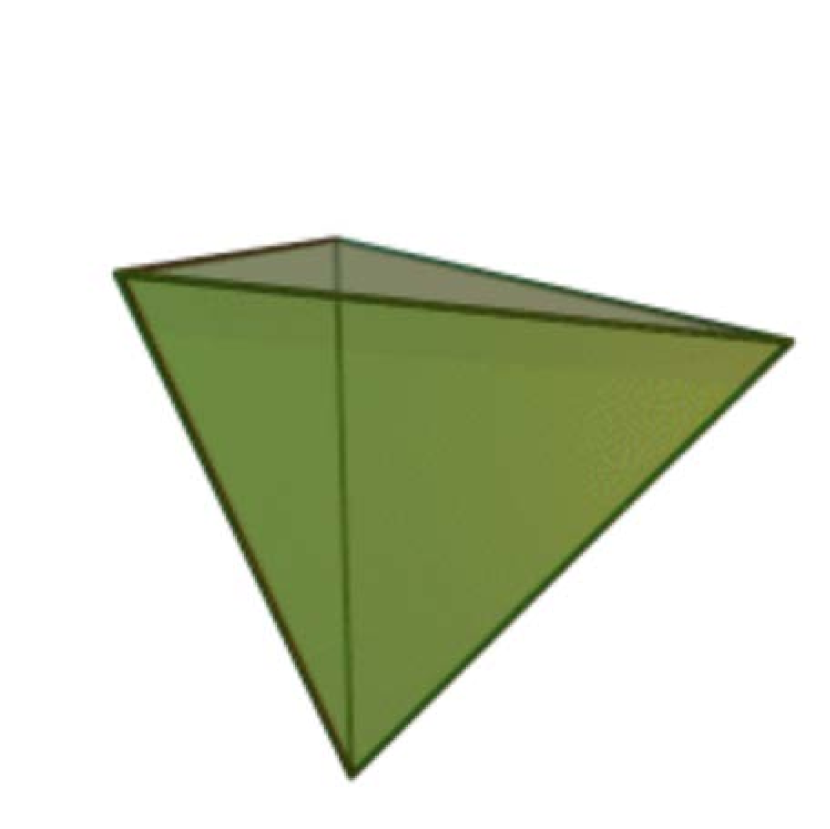
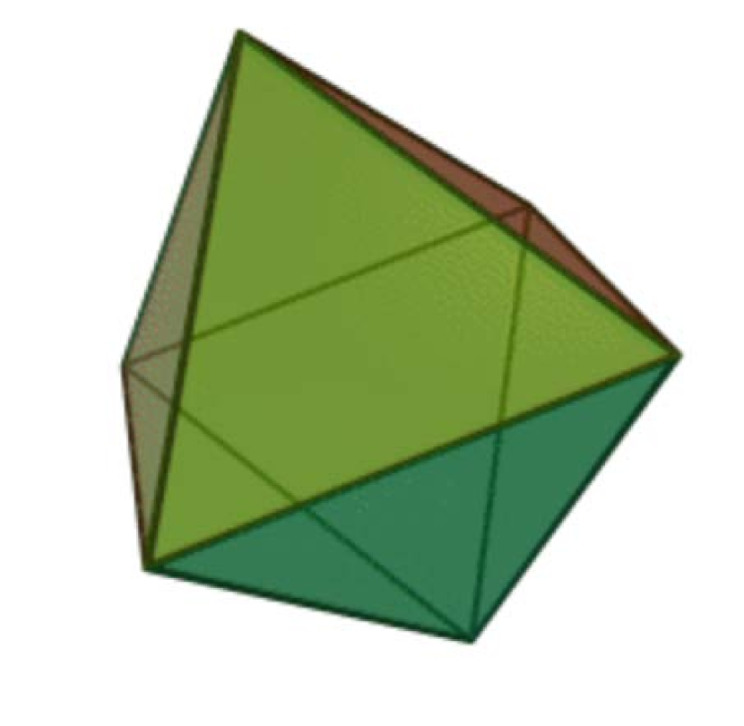
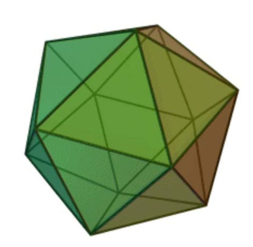
Figure 11: A tetrahedron, an octahedron and an icosahedron, (From Wikipedia, Platonic solid)

We remark that the groups ${\mathcal{A}}_{4}$, ${\mathcal{S}}_{4}$, ${\mathcal{A}}_{5}$ are the groups of symmetry of Platonic solids (see Figure 11 from Wikipedia, Platonic solids).

Proposition 2

There exists a canonical embedding of $SO(3)$ into $PSL(2,\hbox{\bb C})$.

A classical proof of Proposition 2 consists of using the algebra of quaternions. A more geometrical proof can be done as follows : Via the stereographic projection $s$ described in section 3.2, any rotation of the sphere $\hbox{\bb S}^{2}$ can be transported to a bijection from $\hat{\hbox{\bb C}}$ to itself. A direct computation shows that this bijection belongs to $PSL(2,\hbox{\bb C})$.

Proposition 2 implies that we can consider $SO(3)$ as a subgroup of $PSL(2,\hbox{\bb C})\simeq PGL(2,\hbox{\bb C})$.

1.3 The finite subgroups of $PSL(2,\hbox{\bb C})$

Theorem 2 can be extent to the finite subgroups of $PSL(2,\hbox{\bb C})$. We identify $SO(3)$ with its image by the embedding given in Proposition 2. Let $\mu_{n}^{*}$ denote the set of primitive roots of unity in ℂ, and define the equivalence relation $\sim$ on $\mu_{n}^{*}$ by

$$z\sim z^{\prime}\iff z^{\prime}\in\{z,z^{-1}\}.$$

Proposition 3

Let $h\in PSL(2,\hbox{\bb C})),h\neq{\rm Id}$.

1. If the order of $h$ is finite, then $h$ has two fixed points in $\hat{\hbox{\bb C}}$.

2. 1. The following assertions are equivalent :

      1. The order of $h$ is $n>1$;

      2. $h$ is conjugate to a homothecy $z\to\zeta z$, where $[\zeta]\in\mu_{n}^{*}/\sim$.

   2. The space $\mu_{n}^{*}/\sim$ classify the conjugacy classes of order $n$.

Theorem 3

1. Each finite subgroup of $PSL(2,\hbox{\bb C})$ is isomorphic to one of the following groups : A cyclic group $\hbox{\bb Z}_{n}$, a diedral group ${\mathcal{D}}_{n}$, the symmetric group ${\mathcal{S}}_{4}$, the alternate group ${\mathcal{A}}_{4}$, the alternate group ${\mathcal{A}}_{5}$.

2. All subgroups of one of these categories are conjugate in $PSL(2,\hbox{\bb C})$. In particular, they are conjugate to a subgroup of $SO(3,\hbox{\bb R})$.

The canonical embedding of $SO(3)$ into $PSL(2,\hbox{\bb C})$ and item 2 of 3 allows to choose a particular ”standard” element of $SO(3)$ to represent each conjugacy class of a finite subgroup of $PSL(2,\hbox{\bb C})$. This is the goal of Lemma 1. If $h,k\in PSL(2,\hbox{\bb C})$, we denote by $\langle h,k\rangle$ the subgroup spent by $h$ and $k$.

Lemma 1

The following subgroups of $PSL(2,\hbox{\bb C})$ are included in $SO(3)$ :

• ${\bf C}_{n}=\langle z\to\zeta z\rangle$, where $[\zeta]\in\mu_{n}^{*}/\sim$;

• ${\bf D}_{n}=\langle z\to\zeta z,z\to\frac{1}{z}\rangle$, where $\zeta\in\mu_{n}^{*}/\sim$;

• ${\bf A}_{4}=\langle z\to jz,z\to\frac{z+\sqrt{2}}{\sqrt{2}z-1}\rangle$;

• ${\bf S}_{4}=\langle z\to\iota z,z\to\frac{z+1}{z-1}\rangle$;

• ${\bf A}_{5}=\langle z\to\iota z,z\to\frac{z+\Delta}{\Delta z-1}\rangle$, where $\delta$ is a fifth primitive root of unity, and $\Delta=\sqrt{1-\delta-\frac{1}{\delta}}$.

Theorem 4

1. The cyclic subgroups of order $n$ of $PSL(2,\hbox{\bb C})$ are conjugate to the subgroup ${\bf C}_{n}$;

2. The diedral groups of order $n$ are conjugate to the subgroup ${\bf D}_{n}$;

3. The subgroups of $PSL(2,\hbox{\bb C})$ isomorphic to ${\mathcal{A}}_{4}$ are conjugate to the subgroup ${\bf A}_{4}$;

4. The subgroups of $PSL(2,\hbox{\bb C})$ isomorphic to ${\mathcal{S}}_{4}$ are conjugate to the subgroup ${\bf S}_{4}$;

5. The subgroups of $PSL(2,\hbox{\bb C})$ isomorphic to ${\mathcal{A}}_{5}$ are conjugate to the subgroup ${\bf A}_{5}$.

We remind that

• ${\mathcal{A}}_{4}\simeq\langle(123),(12)(34)\rangle$;

• ${\mathcal{S}}_{4}\simeq\langle(1234),(12)\rangle$;

• ${\mathcal{A}}_{5}\simeq\langle(12345),(12)(34)\rangle$.

For further use, we need to compute the normalizers of the finite subgroups of $SO(3)$. If $K$ is a finite subgroup of $SO(3)$, we denote by $N(K)$ its normalizer in $PSL(2,\hbox{\bb C})$. We have the following result ([2] for instance) :

Theorem 5

1. The normalizer in $PSL(2,\hbox{\bb C})$ of any non cyclic finite subgroup of $SO(3)$ is finite and included in $SO(3)$ .

2. More precisely,

   • for any $n\in\hbox{\bb N}^{*}$, $N({\bf D}_{n})={\bf D}_{n}$,

   • $N({\bf A}_{4})={\bf S}_{4}$,

   • $N({\bf S}_{4})={\bf S}_{4}$,

   • $N({\bf A}_{5})={\bf A}_{5}$.

We remark however that the normalizer of a cyclic subgroup ${\bf C}_{n}$ is isomorphic to the group of $2\times 2$ diagonal matrices with complex coefficients. In particular, it is not finite, nor in $SO(3)$.

2 Conformal and holomorphic maps in the Euclidean plane

We denote by $\hbox{\bb E}^{2}$ the (oriented) Euclidean space, that is, the oriented real two dimensional vector space $\hbox{\bb R}^{2}$ endowed with its standard scalar product $g_{\hbox{\bb E}^{2}}$. In the following, we identify $\hbox{\bb E}^{2}$ with ℂ, endowed with the standard scalar product $g_{\hbox{\bb C}}$.

2.1 Conformal maps

Let $U$ and $V$ be open subsets of $\hbox{\bb E}^{2}$.

Definition 1

let $f:U\to V$ be a map.

• The map $f$ is called conformal if it preserves the angles, that is, if it satisfies the following property : For all $p\in U$, any $X_{p}\in T_{p}\hbox{\bb E}^{2}$ and $Y_{p}\in T_{p}\hbox{\bb E}^{2}$,

  $$\angle(f_{p}(X_{p}),f_{p}(Y_{p}))=\angle(X_{p},Y_{p}).$$ (1)

• The map $f$ is called anti-conformal if it preserves the absolute values of the angles (computed in $]-\pi,+\pi[$), and reverses the orientation.

• A bijective conformal map is called a conformal transformation.

In other words, if $g_{0}$ denotes the scalar product of $\hbox{\bb E}^{2}$, a map $f:U\to V$ is conformal if there exists a real function $\lambda$ defined on $U$ such that or all $p\in U$, for all $X_{p}\in T_{p}\hbox{\bb E}^{2}$ and $Y_{p}\in T_{p}\hbox{\bb E}^{2}$,

$$g_{0}(f_{p}(X_{p}),f_{p}(Y_{p}))=e^{\lambda}g_{0}(X_{p},Y_{p}).$$

We can remark that a conformal transformation preserves the orientation. A map $f$ is anticonformal if and only if $\bar{f}$ is conformal. The link between conformal maps and holomorphic map is the following (we identify $\hbox{\bb E}^{2}$ with ℂ) :

Proposition 4

A map $f:U\to V$ is conformal if and only if it is holomorphic and satisfies $f^{\prime}(p)\neq 0$ for every $p\in U$.

In particular, $f$ is a conformal transformation if and only if $f$ is biholomorphic (that is, $f$ and $f^{-1}$ are holomorphic).

2.2 Some reminders on holomorphic maps

Let us recall the well known properties on holomorphic maps defined on a domain $D$. We will use the following theorems :

Theorem 6

Let $D$ be a domain of ℂ, $p\in D$. If $f$ is a holomorphic function defined on $D\backslash\{p\}\subset\hbox{\bb C}$, and bounded on a neighborhood of $p$, then $f$ can be extended as a holomorphic function on $D$.

Theorem 7

If $f$ is a continuous map defined on a domain $D\subset\hbox{\bb C}$, holomorphic on $D$ except at most at the points of a straight line, then $f$ is holomorphic at every point of $D$.

In particular, if $f$ is a continuous function defined on a domain $U\subset\hbox{\bb C}$, holomorphic on $U$ except at most at a finite subset of points, then $f$ is holomorphic at every point of $U$.

Theorem 8

- The Riemann mapping Theorem - If $U$ is a non-empty simply connected open subset of ℂ, different to ℂ, then there exists a biholomorphic bijection $f$ from $U$ onto the open unit disk

$$D=\{z\in\hbox{\bb C},|z|<1\}.$$

As a consequence of Theorem 8, a non-empty simply connected open subset $U$ of ℂ, different to ℂ is also biholomorphic to the upper plane $\hbox{\bb C}^{+}=\{(x,y),y\geq 0\}$ of ℂ, since this upper plane is itself a simply connected open subset $U$ of ℂ different to ℂ. Although Theorem 8 is a purely a existence theorem, the following Schwarz-Christoffel Theorem gives an explicit expression of the biholomorphism from $U$ to the upper plane of ℂ, when $U$ is a polygonal region.

Theorem 9

- The Schwarz-Christoffel Theorem - Let $P$ be a polygonal region in ℂ, with $n$ vertices and interior angles $\alpha_{1},\alpha_{2},...,\alpha_{n}$. The primitive of the function

$$f(z)=A(z-x_{1})^{\frac{\alpha_{1}}{\pi}-1}(z-x_{1})^{\frac{\alpha_{2}}{\pi}-2}...(z-x_{n})^{\frac{\alpha_{1}}{\pi}-n}$$ (2)

(where $A$ is a nonzero constant), maps the upper half plane $\hbox{\bb C}^{+}$ to $P$, in such a way that the real axis is sent on the edges of $P$, and the points $x_{1},\ldots,x_{n}$ on the real axis are sent on the vertices of $P$.

Of course, if the polygonal region is bounded, only $n-1$ angles are included in the formula 2. As an example, if $t$ is a right triangle with angle $\frac{\pi}{6},\frac{\pi}{3},\frac{\pi}{2}$, then a possible mapping $f$ mapping $t$ onto $\hbox{\bb C}^{+}$ is a primitive of the function

$$f(z)=\frac{1}{z^{\frac{1}{2}}(z+1)^{\frac{2}{3}}}.$$

3 Riemann surfaces

3.1 Definition of Riemann surfaces

A Riemann surface is a complex $1$-dimensional analytic manifold. Let us be more precise :

Definition 2

Let $X$ be an (connected oriented) topological surface endowed with an atlas $\{(U_{\alpha},z_{\alpha},V_{\alpha})\}_{\alpha\in I}$, where $\{U_{\alpha}\}_{\alpha\in I}$ covers $X$ by open subsets and for every $\alpha$,

$$z_{\alpha}:U_{\alpha}\to V_{\alpha}\subset\hbox{\bb E}^{2}\simeq\hbox{\bb C}$$

is a homeomorphism from $U_{\alpha}$ onto an open set $z_{\alpha}(U_{\alpha})$, such that, if $U_{\alpha}\cap U_{\beta}\neq\emptyset$,

$$z_{\beta}\circ z_{\alpha}^{-1}:z_{\alpha}(U_{\alpha}\cap U_{\beta})\to z_{\beta}(U_{\alpha}\cap U_{\beta})$$

is a conformal transformation. The surface $X$ is called a Riemann surface. One says that $X$ is endowed with a conformal structure.

In other words, a Riemann surface is a (connected) topological surface whose transition functions are conformal bijections between open subsets of ℂ. Such an atlas is called a complex or conformal atlas. If the union of two conformal atlases on $X$ is still a conformal atlas, they are called equivalent. An equivalence class of conformal atlas is called a conformal structure on $X$. We will denote by the generic letter ${\mathcal{C}}$ the conformal structure defining a Riemann surface.

Two Riemann surfaces are said to be isomorphic if there exists a biholomorphic bijection from the first one to the second one. An automorphism of a Riemann surface $X$ is an isomorphism from $X$ to itself.

Definition 3

Let $X_{1}$ and $X_{2}$ be Riemann surfaces. A map $f:X_{1}\to X_{2}$ is called conformal (resp. holomorphic) at a point $p\in X_{1}$ if there exists a chart $(U_{1},\phi_{1},V_{1})$ around $p$, a chart $(U_{2},\phi_{2},V_{2})$ around $f(p)$ such that $\phi^{-1}_{2}\circ f\circ\phi^{1}_{1}$ is conformal (resp. holomorphic).

3.2 The Riemann uniformization theorem

The following standard surfaces are endowed with a canonical structure of Riemann surface :

• ℂ (it is obvious !)

• Any connected open set of ℂ and in particular the hyperbolic plane

  $$\hbox{\bb H}=\{z\in\hbox{\bb C};\mbox{im}(z)>0\},$$

  that is, the upper half plane of ℂ, isomorphic (as a Riemann surface) to the unit (open) disc $\hbox{\bb D}=\{z\in\hbox{\bb C};|z|<1\}$;

• The Riemann sphere $\hat{\hbox{\bb C}}$ whose underlying set is $\hbox{\bb C}\cup\infty$ endowed with an atlas of two charts : $(U_{1}=\hbox{\bb C},\varphi_{1},V_{1}=\hbox{\bb C}),(U_{2}=\hbox{\bb C}^{*}\cup\{\infty\},\varphi_{2},V_{2}=\hbox{\bb C}^{*}\cup\{\infty\})$, where $\varphi_{1}=id$ and $\varphi_{2}$ is defined by

  $$\begin{cases}\varphi_{2}(z)=\frac{1}{z},\mbox{ {\rm if} }z\in\hbox{\bb C}\\ \varphi_{2}(\infty)=\infty\end{cases}$$

  The transition function is the function

  $$\psi:\hbox{\bb C}^{*}\to\hbox{\bb C}^{*},$$

  defined by $\psi(z)=\frac{1}{z}$. The Riemann surface $\hat{\hbox{\bb C}}$ is a topological $2$-sphere (in particular it is connected and compact), as it is easily shown by the stereographic projection that we describe now : One identifies $\hbox{\bb R}^{3}$ with $\hbox{\bb C}\times\hbox{\bb R}$, we denote by $\hbox{\bb S}^{2}$ its unit sphere, ℂ being the ”horizontal plane”. The north pole $n$ is the point $(0,1)$. The stereographic projection is the map

  $$s:\hbox{\bb S}^{2}\subset\hbox{\bb C}\times\hbox{\bb R}\to\hat{\hbox{\bb C}},$$

  defined for every point $m$ on $\hbox{\bb S}^{2}$ by

  $$\begin{cases}s(m)&=nm\cap\hbox{\bb C},\mbox{ {\rm if} }m\neq n,\\ s(n)&=\infty,\end{cases}$$

  where $nm$ denotes the line throwing $n$ and $m$. The map $s$ is an homeomorphism defined as follows : for all $(z,t)\in\hbox{\bb C}\times\hbox{\bb R}$ such that $|z|^{2}+t^{2}=1$,

  $$s(z,t)=\frac{z}{1-t}.$$

  Its inverse

  $$s^{-1}:\hat{\hbox{\bb C}}\to\hbox{\bb S}^{2}\subset\hbox{\bb C}\times\hbox{\bb R}$$

  satisfies : for all $z\in\hbox{\bb C}$,

  $$s^{-1}(z)=\Big{(}\frac{2z}{|z|^{2}+1},\frac{|z|^{2}-1}{|z|^{2}+1}\Big{)}.$$

  In the following, we will systematically identify $\hat{\hbox{\bb C}}$ and $\hbox{\bb S}^{2}$ via this stereographic projection (justifying the term Riemann sphere for $\hat{\hbox{\bb C}}$.

The three surfaces ℂ, ${\hat{\hbox{\bb C}}}$ and ℍ admit a canonical structure of simply connected Riemann surface. They are the only possible ones, as claimed by the famous following result :

Theorem 10

- Riemann uniformization Theorem - Every complete simply connected Riemann surface is biholomorphic to ℂ, ℍ or $\hat{\hbox{\bb C}}$.

When no confusion is possible, we will denote each of these spaces by the generic letter $\bf H$.

3.3 Fundamental results on compact Riemann surfaces

We mention here three fundamental results in the theory of Riemann surfaces (without proof). Two of them will be useful for the rest of these notes.

Theorem 11

Every (compact oriented) Riemann surface $X$ admits non constant meromorphic maps $f:X\to\hbox{\bb C}$.

Corollary 1

Every (compact oriented) Riemann surface $X$ admits non constant holomorphic maps into $\hat{\hbox{\bb C}}$

$$f:X\to\hat{\hbox{\bb C}}.$$

Corollary 2

Every (compact oriented) Riemann surface $X$ admits a (generally ramified) holomorphic covering over $\hat{\hbox{\bb C}}$.

Theorem 12

Let $X$ be a (compact oriented) Riemann surface. Then, there exists an irreducible polynomial $P\in\hbox{\bb C}[X,Y]$ such that $X$ is isomorphic to the compactification of the regular points of the algebraic curve of equation $P(x,y)=0$.

Theorem 13

Let $X$ be a (compact oriented) Riemann surface. Then there exists an holomorphic embedding of $X$ into ${\hbox{\bb C}}P(3)$.

Although we will not use Theorem 13 in the rest of these notes, we remark that it implies that any (compact connected) Riemann surface appears as a $2$-dimensional real surface minimally embedded in the projective space (of real dimension $6$) ${\hbox{\bb C}}P(3)$.

4 The structure of $\mbox{Aut}(\bf H)$

The following result describes the group $\mbox{Aut}(\bf H)$ of (biholomorphic) automorphisms of $\bf H$ :

Theorem 14

1. One has :

   $$\mbox{\rm Aut}(\hbox{\bb C})=\{z\to az+b,a,b\in\hbox{\bb C}\};$$

2. One has :

   $$\mbox{\rm Aut}(\hbox{\bb H}) =\{z\to\frac{az+b}{cz+d},a,b,c,d\in\hbox{\bb R},ad-bc=1\}$$

   $$\simeq\{\begin{pmatrix}a&b\\ c&d\end{pmatrix};a,b,c,d\in\hbox{\bb R},ad-bc=1\}$$

   $$=PSL(2,\hbox{\bb R}).$$

3. One has :

   $$\mbox{\rm Aut}(\hat{\hbox{\bb C}}) =\{z\to\frac{az+b}{cz+d},a,b,c,d\in\hbox{\bb C},ad-bc=1\}$$

   $$\simeq\{\begin{pmatrix}a&b\\ c&d\end{pmatrix};a,b,c,d\in\hbox{\bb C},ad-bc=1\}$$

   $$=PSL(2,\hbox{\bb C})\simeq PGL(2,\hbox{\bb C}).$$

An element of $\mbox{\rm Aut}(\hbox{\bb C})$ is called an affine map (or an homothecy if $b=0$), an element of $\mbox{\rm Aut}(\hbox{\bb H})$ or $\mbox{\rm Aut}(\hat{\hbox{\bb C}})$ is called an homography. An element of $\mbox{\rm Aut}(\hat{\hbox{\bb C}})$ is also called a Moebius transformation. For further use, we give the following crucial result.

Theorem 15

Let $a$, $b$, $c$ be three (distinct) points of $\hat{\hbox{\bb C}}$. Then there exists a unique Moebius transformation sending $0$ to $a$, $1$ to $b$ and $\infty$ to $c$.

Now, one can build an action of the group $PSL(2,\hbox{\bb C})$ on $\hat{\hbox{\bb C}}$ as follows : for any matrix $\begin{pmatrix}a&b\\ c&d\end{pmatrix}$, where $(a,b,c,d\in\hbox{\bb C},ad-bc=1)$,

$$\begin{pmatrix}a&b\\ c&d\end{pmatrix}.z=\frac{az+b}{cz+d}.$$

In the next sections, we will systematically use Proposition 1 and Theorem 14 : ${\rm Aut}(\hat{\hbox{\bb C}})\simeq PGL(2,\hbox{\bb C})$.

5 Classification of Riemann surfaces

5.1 Description of Riemann surfaces with respect to their genus

If $X$ is any Riemann surface, $X$ is the quotient of its universal covering $\bf H$ by a subgroup of $\mbox{Aut}({\bf H})$ acting freely an discontinuously on ${\bf H}$. Since the covering is holomorphic, the covering automorphisms are holomorphic and then, Riemann surfaces can be classified as follows :

Theorem 16

Let $X$ be a Riemann surface of genus ${\bf g}_{X}$.

1. If ${\bf g}_{X}=0$ then $X=\hat{\hbox{\bb C}}$.

2. If ${\bf g}_{X}=1$, then $X$ is a quotient $\hbox{\bb C}/\Gamma$, where $\Gamma$ is a lattice $u\hbox{\bb Z}\oplus v\hbox{\bb Z}$, acting on ℂ by translations, where $u$ is a complex number, $v$ is a nonzero complex number, such that $\frac{u}{v}$ is not a real number.

3. If ${\bf g}_{X}>1$, then $X$ is a quotient $\hbox{\bb H}/\Gamma$, where $\Gamma$ is a Fuchsian subgroup of $PSL(2,\hbox{\bb R})$ (that is, a subgroup acting freely and properly discontinuously on ℍ).

5.2 Modular spaces

Let $X$ be a closed oriented surface, and ${\mathcal{M}}$ be the set of conformal structures ${\mathcal{C}}$ on $X$. Let $\sim$ be the equivalence relation defined on ${\mathcal{M}}$ as follows : Two conformal structures ${\mathcal{C}}_{1}$ and ${\mathcal{C}}_{2}$ on $X$ are equivalent when there exists a conformal diffeomorphism

$$\phi:(X,{\mathcal{C}}_{1})\to(X,{\mathcal{C}}_{2}).$$

Definition 4

The quotient space ${\mathcal{M}}/\sim$ is called the modular space of conformal structures of $X$.

The modular spaces of conformal structures of a given genus have a structure of complex manifold. More precisely, the modular space $\mathcal{M}_{{\bf g}}$ (of conformal structures defined on a - closed oriented - surface of genus ${\bf g}>1$) has a structure of a complex manifold of dimension $3g-3$, and the modular space $\mathcal{M}_{1}$ can be identified to $\hbox{\bb H}/PSL(2,\hbox{\bb Z})$. For ${\bf g}=0$, one has the following result :

Theorem 17

The modular space $\mathcal{M}_{0}$ is reduced to a point.

Although we don’t give a direct proof of Theorem 17, we remark that it is an easy consequence of the Riemann-Roch theorem : On any (oriented closed) surface $X_{0}$ of genus $0$, there exists a meromorphic function with one pole of degree one.

On the other hand, Theorem 17 means that $X_{0}$ is conformally equivalent to the Riemann sphere $\tilde{\hbox{\bb C}}$. Consequently, we can call a (closed oriented) Riemann surface $X_{0}$ with genus $0$, the Riemann sphere. Concretely, Theorem 17 means that if ${\mathcal{C}}_{1}$ and ${\mathcal{C}}_{2}$ are two conformal structures on $X_{0}$, there exists a conformal diffeomorphism (or a biholomorphism preserving the orientation) from $(X_{0},{\mathcal{C}}_{1})$ to $(X_{0},{\mathcal{C}}_{2})$.

6 Riemannian surfaces

A Riemannian surface $(X,g)$ is a $2$-dimensional real (smooth) surface, endowed with a (smooth) Riemannian metric $g$. By definition, this means that $X$ is endowed with an atlas ${\mathcal{A}}=\{(U_{\alpha},\phi_{\alpha},V_{\alpha}\subset\hbox{\bb R}^{2})\}$ where each $V_{\alpha}$ is endowed with a metric (symmetric positive definite bilinear form) $g_{\alpha}$ such that the transition functions

$$\phi_{\beta}\circ\phi_{\alpha}^{-1}:(\phi_{\alpha}(U_{\alpha}\cap U_{\beta}),g_{\alpha})\to(\phi_{\beta}(U_{\alpha}\cap U_{\beta},g_{\beta}))$$

are isometries. In the following, as usual, we identify $g$ on $U_{\alpha}$ and its local representation $g_{\alpha}$ on $V_{\alpha}$.

6.1 Isothermal coordinates

In local coordinates $(x,y)$ in each $U_{i}$, the metric $g$ defined on a Riemann surface can be written as follows :

$$g=Edx^{2}+2Fdxdy+Gdy^{2},$$

where $E$, $F$, $G$ are real valued functions of the variables $x$ and $y$. Using complex coordinates $z=x+iy$,

$$g=\alpha|dz+\mu d\bar{z}|^{2},$$

where $\alpha$, $\mu$, are real valued functions of the variables $z$ and $\bar{z}$. Gauss (in the analytic case), Korn and Lichtenstein (in the smooth case) proved that it is always possible to find a (local) system of coordinates $(u,v)$ on $U_{i}$ so that

$$g=e^{\lambda}(du^{2}+dv^{2}),$$ (3)

or, using complex coordinates $w=u+iv$,

$$g=e^{\lambda}dwd\bar{w}.$$

Such coordinates are called isothermal coordinates. This result can be stated as follows :

Theorem 18

Let $(X,g)$ be a Riemannian surface. Then, around each point $p\in X$, there exists a chart $(U,\phi,V)$ and a smooth function $\lambda$ such that $g|U=e^{\lambda}g_{\hbox{\bb E}^{2}}$, where $g_{\hbox{\bb E}^{2}}$ denotes the standard scalar product on $V\subset\hbox{\bb E}^{2}$.

A chart satisfying 3 is called an isothermal chart.

The following result is obvious but important :

Proposition 5

The transition functions of the atlas ${\mathcal{A}}$ defined on an (oriented) Riemannian surface $(X,g)$, restricted to isothermal charts are conformal maps

$$\phi_{\beta}\circ\phi_{\alpha}^{-1}:\phi_{\alpha}((U_{\alpha}\cap U_{\beta},g_{\hbox{\bb E}^{2}}))\to\phi_{\beta}((V_{\alpha}\cap V_{\beta},g_{\hbox{\bb E}^{2}})).$$

Proof of Proposition 5 - Indeed, let $\phi=\phi_{\beta}^{-1}\circ\phi_{\alpha}$. Denoting for all $\alpha\in I$, $g_{\alpha}=g|U_{\alpha}$, we have

$$g_{\alpha}=e^{\lambda_{\alpha}}g_{\hbox{\bb E}^{2}},g_{\beta}=e^{\lambda_{\beta}}g_{\hbox{\bb E}^{2}},$$

where $\lambda_{\alpha}$ and $\lambda_{\beta}$ are smooth functions, because $(U_{\alpha},\phi_{\alpha})$ and $(U_{\beta},\phi_{\beta})$ are isothermal charts. On the other hand, by definition of $g$,

$$\phi^{*}(g_{\beta})=g_{\alpha}.$$

We deduce that

$$e^{\lambda_{\alpha}}g_{\hbox{\bb E}^{2}}=g_{\alpha}=\phi^{*}(g_{\beta})=\phi^{*}(e^{\lambda_{\beta}}g_{\hbox{\bb E}^{2}})=e^{\lambda_{j}}\phi^{*}(g_{\hbox{\bb E}^{2}}),$$

from which we deduce that

$$\phi^{*}(g_{\hbox{\bb E}^{2}})=e^{\lambda_{\alpha}-\lambda_{\beta}}g_{\hbox{\bb E}^{2}},$$

implying that the transition functions $\phi=\phi_{\beta}^{-1}\circ\phi_{\alpha}$ are conformal.

6.2 Conformal class of a metric

Two Riemannian metrics $g$ and $h$ defined on a surface $X$ are called conformal if $g=e^{\lambda}h$, where $\lambda:X\to\hbox{\bb R}$ is a $C^{\infty}$ function. One can classify the Riemannian metrics by defining an equivalence relation as follows: Two Riemannian metrics $g$ and $h$ defined on $X$ are equivalent if they are conformal. For further use, we state the following lemma that gives the relation between the (Gaussian) curvatures of two conformal metrics.

Lemma 2

Let $(X,g)$ be a closed oriented Riemannian surface with curvature $k_{g}$, and $h$ a metric on $X$ conformal to $g$ with (Gaussian) curvature $k_{h}$ : There exists a smooth function $\lambda$ on $X$ such that

$$h=e^{\lambda}g.$$

Then,

$$k_{h}=e^{-\lambda}(k_{g}-\Delta_{g}\lambda),$$ (4)

where $\Delta_{g}$ is the Laplacian of $g$.

6.3 Riemannian surfaces versus Riemann surfaces

The link between Riemannian surfaces and Riemann surfaces can be summarized as follows :

Theorem 19

Let $X$ be an (differentiable) surface. It is equivalent to endow $X$ with a complex structure or to endow it with an orientation and a conformal equivalence class of Riemannian metrics.

By a complex structure, we mean a (maximal) atlas whose transition functions are conformal.

Sketch of Proof of Theorem 19 - Let us describe now the main steps of the proof of Theorem 19 and how the bijection is built.

• Let us show how a conformal structure on $X$ determines a natural conformal class of Riemannian metrics on $X$ : On an atlas $\mathcal{A}$, one defines a locally finite partition of unity $\mu_{\alpha}$, the support of each $\mu_{\alpha}$ being included in a chart $(U_{\alpha},\phi_{\alpha},V_{\alpha})$ of $\mathcal{A}$. One endows each $U_{\alpha}$ with the natural Euclidean metric $\phi_{\alpha}^{-1}(g_{\alpha})$, where $g_{\alpha}$ is the restriction on $V_{\alpha}$ of the Euclidean metric on $\hbox{\bb C}\simeq\hbox{\bb E}^{2}$. Then, we define on $X$ the Riemannian metric $g=\sum\mu_{\alpha}\phi_{\alpha}^{-1}(g_{\alpha})$ on $X$. Any metric $h=e^{\lambda}g$ conformal to $g$ (where $\lambda$ is a smooth function) can be obtained by the same process (multiplying each $\mu_{i}$ by $e^{\lambda}$). Consequently, we have associated to any Riemann structure on $X$ a conformal class of Riemannian metrics. Moreover, one proves that the class of Riemannian metrics giving rise to a given complex structure on $X$ is exactly a conformal class of Riemannian metrics.

• Conversely, if $(X,g)$ is an (oriented) Riemannian surface, one builds an isothermal atlas $\mathcal{A}=\{(U_{\alpha},\phi_{\alpha},V_{\alpha}),\alpha\in I\}$ of $X$. Then we apply Proposition 5. We conclude immediately that $X$ admits a structure of Riemann surface. By construction, two conformal metrics give rise to the same conformal structure.

The previous correspondences are inverse one to each other, Theorem 19 is proved.

Definition 5

A metric $g$ defined on a Riemann surface $X$ is said to be compatible with its conformal structure if this conformal structure is induced by $g$.

We conclude this section by the following remark : Let $g_{1}$ (resp. $g_{2}$) be a Riemannian metric on a (closed oriented) surface $X_{0}$ of genus $0$. Let ${\mathcal{C}}_{1}$ (resp. ${\mathcal{C}}_{2}$) be the conformal structure associated to $g_{1}$ (resp. $g_{2}$). From Theorem 17, we know that there exists a conformal diffeomorphism

$$\phi:(X_{0},g_{1})\to(X_{0},g_{2}).$$

Using Theorem 17 and Theorem 19, we get the following Riemannian result :

Corollary 3

Let $g_{1}$ (resp. $g_{2}$) be a Riemannian metric on a (closed oriented) surface $X_{0}$ of genus $0$. Let ${\mathcal{C}}_{1}$ (resp. ${\mathcal{C}}_{2}$) be the conformal structure associated to $g_{1}$ (resp. $g_{2}$). Then, there exists a biholomorphism

$$\phi:(X_{0},g_{1})\to(X_{0},g_{2}),$$

that is, there exists a diffeomorphism $\phi$ of $X_{0}$ and a smooth function $\lambda$ on $X_{0}$ such that, $\phi^{*}(g_{2})=e^{\lambda}g_{1}$.

Indeed, $g_{1}$ (resp. $g_{2}$) induces a conformal structure ${\mathcal{C}}_{1}$ (resp. ${\mathcal{C}}_{2}$). Since Theorem 17 claims that the modular space of $X_{0}$ is reduced to a point, there exists a conformal diffeomorphism

$$\phi:(X_{0},{\mathcal{C}}_{1})\to(X_{0},{\mathcal{C}}_{2}),$$

and then, there exists a smooth function $\lambda$ such that $\phi^{*}(g_{2})=e^{\lambda}g_{1}$.

7 Metrics of constant Gaussian curvature

7.1 The simply connected case

When $X$ is simply connected, one can give an explicit description of the metrics with constant curvature on $X$. We begin with the famous theorem of Cartan :

Theorem 20

- The uniformization theorem of Cartan in Riemannian geometry - Let $(X,g)$ be a connected, complete, simply connected, oriented Riemannian surface with constant Gaussian curvature $k$.

• If $k=1$, then $(X,g)$ is isometric to the round sphere of radius $1$.

• If $k=0$, then $(X,g)$ is isometric to the Euclidean plane.

• If $k=-1$, then $(X,g)$ is isometric to the hyperbolic plane (endowed with its canonical metric of constant curvature $-1$).

Remark that these isometries are not unique since they are parametrised by isometric automorphisms of $(X,g)$. On the other hand, the three spaces described in Theorem 20 (the sphere, the plane, the hyperbolic plane), admits by Theorem 10 a canonical complex structure. We now describe these three situations.

1. Let us study the case $k=0$, and identify the plane with ℂ. The metric $g_{\hbox{\bb C}}=|dz^{2}|$ is the canonical flat Riemannian metric on ℂ. Since any biholomorphism of ℂ is an affine map

   $$f:z\to az+b,a\in\hbox{\bb C},b\in\hbox{\bb C},$$

   we can write $f^{*}g_{\hbox{\bb C}}=e^{\lambda}g_{\hbox{\bb C}},\lambda\in\hbox{\bb R}$, from which we deduce a family of flat Riemannian metrics on ℂ associated to the canonical complex structure, conformal to $g_{0}$, parametrised by $\hbox{\bb R}^{*}_{+}$. So, up to a scaling constant, there exists a canonical flat Riemannian metric on ℂ associated to its canonical complex structure.

2. Let us study the case $k=-1$, identifying the hyperbolic plane with ℍ. The Riemannian metric

   $$g_{\hbox{\bb H}}=\frac{|dz|^{2}}{[\mbox{{\rm im}}(z)]^{2}}$$

   has constant Gaussian curvature $-1$. The crucial remark is that $g_{\hbox{\bb H}}$ is invariant by $\mbox{\rm Aut}(\hbox{\bb H})$. In other words, any biholomorphism of ℍ is a $g_{\hbox{\bb H}}$-isometry. We call $g_{\hbox{\bb H}}$ the canonical metric of constant curvature $-1$ on ℍ.

3. Let us study the case $k=1$. Via the stereographic projection $s$, we identify the sphere $\hbox{\bb S}^{2}$ as before with $\hat{\hbox{\bb C}}$. The sphere $\hbox{\bb S}^{2}$ admits a Riemannian metric $g_{\hbox{\bb S}^{2}}$ of constant curvature $1$, induced by the standard scalar product of $\hbox{\bb E}^{3}\simeq\hbox{\bb C}\times\hbox{\bb R}$ :

   $$g_{\hbox{\bb S}^{2}}=\frac{4|dz|^{2}}{(1+|z|^{2})^{2}}.$$

   On $\hat{\hbox{\bb C}}$, a simple computation gives

   $$g_{\hat{\hbox{\bb C}}}=\frac{4|du|^{2}}{(1+|u|^{2})^{2}},$$ (5)

   where $u=\frac{1}{z}$. However, $g_{\hat{\hbox{\bb C}}}$ is not invariant by $\mbox{\rm Aut}(\hat{\hbox{\bb C}})$. Consequently $g_{\hat{\hbox{\bb C}}}$ is not characterised by the Riemann structure of $\hat{\hbox{\bb C}}$. But the curvature of $g_{\hat{\hbox{\bb C}}}$ is preserved by $\mbox{\rm Aut}(\hat{\hbox{\bb C}})$. More precisely, we have the following lemma :

   Lemma 3

   1. If $h\in\mbox{\rm Aut}(\hat{\hbox{\bb C}})$, $h^{*}(g_{\hat{\hbox{\bb C}}})$ is a Riemannian metric with constant curvature $1$.

   2. The family of Riemannian metrics $\tilde{g}$ with constant Gaussian curvature $1$ conformal to the canonical metric $g_{\hat{\hbox{\bb C}}}$ on $\hat{\hbox{\bb C}}$, is naturally endowed with a structure of homogenous space isomorphic to $SO(3)\backslash\mbox{\rm Aut}(\hat{\hbox{\bb C}})\simeq SO(3)\backslash PSL(2,\hbox{\bb C})$.

   3. More generally, if $g$ is any Riemannian metric on $\hat{\hbox{\bb C}}$, the family of Riemannian metrics $\tilde{g}$ with constant Gaussian curvature $1$ conformal to $g$, is naturally endowed with a structure of homogenous space isomorphic to $SO(3)\backslash\mbox{\rm Aut}(\hat{\hbox{\bb C}})\simeq SO(3)\backslash PSL(2,\hbox{\bb C})$.

   Proof of Lemma 3 -

   1. If $h\in\mbox{\rm Aut}(\hat{\hbox{\bb C}})$, $h^{*}(g_{\hat{\hbox{\bb C}}})$ is still a metric with constant curvature $1$, but generally, $h^{*}(g_{\hat{\hbox{\bb C}}})\neq g_{\hat{\hbox{\bb C}}}$. In other words, any biholomorphism of $\hat{\hbox{\bb C}}$ preserves the (constant) curvature of $g_{\hat{\hbox{\bb C}}}$ but does not preserve $g_{\hat{\hbox{\bb C}}}$ in general.

   2. Let $\tilde{g}$ be any metric of constant curvature $1$ on $\hat{\hbox{\bb C}}$. Then, by Theorem 20, there exists an isometry

      $$\psi:(\hat{\hbox{\bb C}},\tilde{g})\to(\hat{\hbox{\bb C}},g_{\hat{\hbox{\bb C}}}).$$

      On the other hand, if we suppose that $\tilde{g}$ is in the conformal class of $g_{\hat{\hbox{\bb C}}}$, there exists a smooth function $\lambda$ such that $\tilde{g}=e^{\lambda}g_{\hat{\hbox{\bb C}}}$. We deduce that

      $$\psi^{*}g_{\hat{\hbox{\bb C}}}=e^{\lambda}g_{\hat{\hbox{\bb C}}},$$

      that is, $\psi$ is a conformal map from $(\hat{\hbox{\bb C}},g_{\hat{\hbox{\bb C}}})$ to $(\hat{\hbox{\bb C}},g_{\hat{\hbox{\bb C}}})$ : $\psi\in\mbox{Aut}(\hat{\hbox{\bb C}})\simeq PSL(2,\hbox{\bb C})$. Now, let $\varphi\in\mbox{Aut}(\hat{\hbox{\bb C}})$. We have

      $$(\varphi\circ\psi)^{*}g_{\hat{\hbox{\bb C}}}=(\psi^{*}\circ\varphi^{*})g_{\hat{\hbox{\bb C}}}=\psi^{*}g_{\hat{\hbox{\bb C}}},$$

      for all $\psi\in\mbox{Aut}(\hat{\hbox{\bb C}})$, if and only if $\varphi\in SO(3)$. The conclusion follows.

   3. The last item is an easy generalization of item 3b : If $g$ is any metric on $\hat{\hbox{\bb C}}$, Theorem 21 claims that there exists a metric $\tilde{g}$ of constant curvature $1$ conformal to $g$. If $\tilde{g}^{\prime}$ is another metric of constant curvature $1$ conformal to $g$, then $\tilde{g}^{\prime}$ is conformal to $\tilde{g}$. We apply item 3b, and the conclusion follows.

7.2 A general uniformization theorem in Riemannian geometry

We consider now closed Riemannian surfaces with any genus. The Poincare-Klein-Koebe uniformization theorem claims that in each conformal class of metrics on a surface $X$, there exists a metric with constant Gaussian curvature $1$, $0$ or $-1$ :

Theorem 21

- Poincare-Klein-Koebe uniformization theorem - Let $(X,g)$ be a closed oriented Riemannian surface of genus ${\bf g}_{X}$. Then, there exists a Riemannian metric $\tilde{g}$ conformal to $g$ with constant Gaussian curvature $-1$, $0$, or $1$.

1. If ${\bf g}_{X}>1$, the Gaussian curvature is $-1$, and $g$ is unique.

2. If ${\bf g}_{X}=1$, the Gaussian curvature is $0$, and $g$ is unique up to a scaling constant.

3. If ${\bf g}_{X}=0$, there exists a family of Riemannian metrics $\tilde{g}$ conformal to $g$ with constant Gaussian curvature $1$.

We will improve Theorem 21 item 3 in section 7.1 Lemma 3 by describing the geometry of the set of metrics with constant curvature $1$ that are conformal to $g$. The proof of Theorem 21 is based on Lemma 2. To find a metric of constant curvature conformal to $g$, one solves equation 4 with $k_{g^{\prime}}=-1,0$ or $1$, that is, one looks for a smooth function $\lambda$ satisfying 4.

Sketch of proof of Theorem 21 - We only give here indications of the proof in the simplest case of genus $1$. Let $X_{1}$ be a surface of genus $1$ endowed with a metric $g$ of curvature $k_{g}$. Let $g^{\prime}=e^{\lambda}g$, where $\lambda$ is a smooth function on $X_{0}$. From equation 4, we deduce that $k_{g^{\prime}}=0$ if and only if

$$\Delta_{g}\lambda=k_{g},$$ (6)

By using the classical theory of autoadjoint operators, we solve equation 6 : Up to a constant, it admits a unique solution.

7.3 Metrics of constant curvature on a Riemann surface of any genus

If we a priori deal with a closed Riemann surface (of any genus), the results of subsection 7.2 can be rephrased as follows :

Theorem 22

Let $X$ be a (closed oriented) Riemann surface of genus ${\bf g}_{X}$. Then,

• If ${\bf g}_{X}>1$, there exists a unique Riemannian metric $\tilde{g}$ with constant Gaussian curvature $-1$, compatible with the complex structure and invariant by $\mbox{\rm Aut}(X)$.

• If ${\bf g}_{X}=1$, there exists a Riemannian metric $\tilde{g}$ with constant Gaussian curvature $0$, unique up to a scaling constant, compatible with the complex structure and invariant by $\mbox{\rm Aut}(X)$.

• If ${\bf g}_{X}=0$, and $g$ is a Riemannian metric on $X$, the family of Riemannian metrics $\tilde{g}$ with constant Gaussian curvature $1$ conformal to $g$ is naturally endowed with a structure of homogenous space isomorphic to $\mbox{\rm Aut}(SO(3)\backslash\hat{\hbox{\bb C}})\simeq SO(3)\backslash PSL(2,\hbox{\bb C})$.

We deduce from Theorem 22 that there exists a natural homogenous space of metrics with constant Gaussian curvature $1$ on $\hat{\hbox{\bb C}}$ : We consider the metric $g_{\hbox{\bb S}^{2}}$ of constant Gaussian curvature $1$ on the round sphere $\hbox{\bb S}^{2}$ of radius $1$. We identify $\hbox{\bb S}^{2}$ with $\hat{\hbox{\bb C}}$ by help of the stereographic projection, and consider the metric $g_{\hat{\hbox{\bb C}}}$ on $\hat{\hbox{\bb C}}$ deduced from $g_{\hbox{\bb S}^{2}}$ by this identification. We then consider the homogenous space of Riemannian metrics $\tilde{g}$ with constant Gaussian curvature $1$ conformal to $g_{\hat{\hbox{\bb C}}}$.

7.4 Metric on $\hat{\hbox{\bb C}}$ associated to a finite subgroup of $\mbox{\rm Aut}(\hat{\hbox{\bb C}})$

The following proposition builds a canonical Riemannian metric on $\hat{\hbox{\bb C}}$ associated to any finite subgroup $K$ of ${\rm Aut}(\hat{\hbox{\bb C}})$ (by Theorem 3, we know that $K$ is conjugate to a (finite) subgroup of $SO(3)$ canonically embedded in $\mbox{\rm Aut}(\hat{\hbox{\bb C}})$ by Proposition 2).

Proposition 6

Let $K$ be a finite subgroup of ${\rm Aut}(\hat{\hbox{\bb C}})$. Then, $\hat{\hbox{\bb C}}$ admits a canonical Riemannian metric $\tilde{g}_{K}$ invariant by $K$, that coincides with the metric $g_{\hat{\hbox{\bb C}}}$ if $K$ is a subgroup of $SO(3)$.

Proof of Proposition 6 - We still denote by $g_{\hat{\hbox{\bb C}}}$ the canonical metric on $\hat{\hbox{\bb C}}$ defined by 5. We define $\tilde{g}_{K}$ as follows : For all $u,v$ in $T\hat{\hbox{\bb C}}$,

$$\tilde{g}_{K}(u,v)=\frac{1}{{\rm card}(K)}\sum_{h\in K}g_{\hat{\hbox{\bb C}}}(dh(u),dh(v)).$$ (7)

For each $h\in K$, Lemma 3 implies that the map

$$(u,v)\to g_{\hat{\hbox{\bb C}}}(dh(u),dh(v))$$

is a metric of constant curvature $1$. Then, $\tilde{g}$ is a metric clearly invariant by $K$. The rest of Proposition 6 is clear.

8 Canonical Riemann structure on a polyhedron

By an (abstract) oriented Euclidean polyhedron, we mean an oriented topological surface obtained as the union of a finite set of disjoint polygonal domains of the Euclidean plane $\hbox{\bb E}^{2}$, after the identification of some of their edges and vertices. Such polyhedra are piecewise linear and admit on each of their face a canonical (Euclidean) flat metric with potential singularities at the vertices. In this section we will build a canonical Riemann structure on any (abstract) Euclidean polyhedron. More precisely, we can claim :

Theorem 23

Any Euclidean polyhedron admits a canonical conformal structure.

Proof of Theorem 23 - Let us build a conformal atlas on the polyhedron $P$ :

• First of all, we consider any point $p$ belonging to the interior of a face $f$ or to the interior of an edge $e$ adjacent to two faces $f$ and $f^{\prime}$. As a domain of chart around $p$, we take any open neighborhood $U$ of $p$ in $f\cup f^{\prime}$, and we send it isometrically onto a neighborhood of $0$ in the Euclidean plane $\hbox{\bb E}^{2}$. Denoting by $\phi$ this isometry, the triple $(U,\phi,\phi(U))$ is a chart around $p$.

• On the other hand, if $v$ is a vertex of the polyhedron, we consider a ”small” neighborhood $U$ of $v$ that is the union of sectors at $p$ surrounding $p$ : Let $e_{1},\ldots,e_{k}$ be the sequence of edges adjacent to $v$, and $\theta_{1},\ldots,\theta_{k}$ the angle between consecutive edges.

  • We send isometrically the interior $\stackrel{{\scriptstyle\circ}}{{f_{i}}}\cap U$ in each face $f_{i}$ to the interior of a sector $V_{i}$ in $\hbox{\bb E}^{2}$ whose vertex is $0$.

  • Now, we apply the transformation $\delta_{i}:z\to z^{\alpha}$, where

    $$\alpha=\frac{2\pi}{\sum_{k}\theta_{i}}.$$

    (This transformation is well defined at every point different to $0$.) In such a way, the $\delta_{i}(\stackrel{{\scriptstyle\circ}}{{f_{i}}}\cap U)$ is a sector $V_{i}$ of angle $\alpha\theta_{i}$.

  • After rotations with suitable angles, the union of the sectors $V_{i}\cup e_{i}$ covers exactly an open neigborhood of $0$ in $\hbox{\bb E}^{2}$ (punctured at $0$), since the sum of the sector angles equals $2\pi$.

  • Therefore, by continuity on the edges and on the vertex $p$, we have built a homeomorphism $\phi$ of $U$ onto an open neighborhood of $0$. We remark that $v$ is sent onto $0$. The triplet $U,\phi,\phi(U)$ is a chart.

  • The set of charts $\{U_{i},\phi_{i},\phi_{i}(U_{i}),i\in I\}$ defined above define an atlas on $P$. Let us study the transition functions. Let $U_{i}$ and $U_{j}$ be two domains of charts.

    • If $U_{i}$ or $U_{j}$ contains no vertices, the transition function

      $$\phi_{j}^{-1}\circ\phi_{i}:\phi_{i}(U_{i}\cap U_{j})\to\phi_{j}(U_{i}\cap U_{j})$$

      is composed of rotations, translations that are holomorphic, and power functions $z\to z^{\alpha}$, that are holomorphic since the origin does not belong to $\phi_{i}(U_{i}\cap U_{j})$.

    • If $U_{i}$ or $U_{j}$ contains a vertex, the transition function

      $$\phi_{j}^{-1}\circ\phi_{i}:\phi_{i}(U_{i}\cap U_{j})\to\phi_{j}(U_{i}\cap U_{j})$$

      is composed of rotations, translations that are holomorphic, and power functions $z\to z^{\alpha}$, that are bounded and holomorphic except at $0$ (where the power function is not defined). Then, by Theorem 6, $\phi_{j}^{-1}\circ\phi_{i}$ can be extended to an holomorphic function on $\phi_{i}(U_{i}\cap U_{j})$.

Therefore, this construction defines a holomorphic structure on $P$.

Figure 1: Angles at a vertex $p$ of the triangles incident to $p$

Figure 2: Modifying the angle of each sector

Figure 3: Flattening a cone

In particular, the (boundary of) any polyhedric body in $\hbox{\bb E}^{3}$ admits a canonical conformal structure.

Theorem 23 can be extent to any triangulation on any (compact oriented) topological surface $X$. Indeed, by assigning the length $1$ to each edge of ${\mathcal{T}}$, $X$ is canonically endowed with a structure of Euclidean polyhedron whose faces are equilateral triangles (the Euclidean structure of each triangle being induced by the ones of the edges). Such a geometric structure will be called an equilateral triangulation). We deduce :

Corollary 4

Any triangulation ${\mathcal{T}}$ defined on a (closed oriented) surface $X$ induces on $X$ a canonical conformal structure: The one defined by the equilateral triangulation.

The following theorem claims that the converse of Theorem 23 is true in the following sense :

Theorem 24

Let $X$ be a (closed oriented) Riemann surface endowed with a conformal structure ${\mathcal{C}}$. Then, there exists on $X$ a Euclidean triangulation ${\mathcal{T}}$ whose associated conformal structure is isomorphic to ${\mathcal{C}}$.

Proof of Theorem 24 -

• The result is trivial if the genus of $X$ is $0$, since the modular space of $X$ is reduced to a point (see Theorem 17).

• Let $X$ be any (closed oriented) Riemann surface. We know that $X$ admits holomorphic (generally ramified) coverings over $\hat{\hbox{\bb C}}$

  $$\pi:X\to\hat{\hbox{\bb C}},$$

  (see Theorem 2). We choose one of them. Let ${\mathcal{T}}^{\prime}$ be any triangulation of $\hat{\hbox{\bb C}}$ satisfying the following property : Any singular value of $\pi$ is a vertex of ${\mathcal{T}}^{\prime}$. Let us endow ${\mathcal{T}}^{\prime}$ with any Euclidean structure. By Theorem 23, it induces the (unique) conformal structure of $\hat{\hbox{\bb C}}$. Moreover, the inverse image of ${\mathcal{T}}^{\prime}$ by $\pi$ is a triangulation ${\mathcal{T}}$ of $X$ such that each triangle $t$ of ${\mathcal{T}}$ is in one to one correspondence with a triangle of ${\mathcal{T}}^{\prime}$. Let us endow each triangle $t$ with the Euclidean metric making the restriction of $\pi$ to $t$ an isometry and then a conformal bijection from $t$ to $\pi(t)$. Let us denote by $\{v_{1},...,v_{n}\}$ the vertices of $\mathcal{T}$ and by $\{w_{1},...,w_{m}\}$ the vertices of ${\mathcal{T}}^{\prime}$. The pullback of the conformal structure of $\hat{\hbox{\bb C}}\backslash\{w_{1},...,w_{m}\}$ by $\pi$ is a conformal structure ${\mathcal{C}}_{1}$ on $X\backslash\{v_{1},...,v_{n}\}$ isomorphic to the restriction of ${\mathcal{C}}$ on $X\backslash\{v_{1},...,v_{n}\}$. Because the set of vertices on ${\mathcal{T}}$ is finite, ${\mathcal{C}}_{1}$ can be extended to $X$, and ${\mathcal{C}}_{1}={\mathcal{C}}$ on $X$.

9 Dessins d’enfants

9.1 Main definitions

Introduction and developments on the theory of dessins d’enfants can be found in [10] [11] [6] [15] [12] [7]. The definition of dessins may differ following the authors. For simplicity, we will use the following ”standard” one:

Definition 6

[7] [15] [12] A dessin d’enfants (or simply a dessin) is a couple $(X,{\mathcal{D}})$, where $X$ is an (oriented) topological surface and ${\mathcal{D}}$ a finite bicolored graph on it such that $X\backslash D$ is a finite union of disjoint topological discs.

Figure 4: A graph on a surface of genus $2$

As any finite graph, a dessin has a finite set of vertices $V$ and a finite set of edges $E$. As a bicolored graph, each vertex can be colored in white or black, in such a way that the colors of two consecutive vertices on the same edge are different.

The definition of a dessin by A. Grothendieck is a little bit more general : One simply considers a graph on a surface $X$ such that $X\backslash D$ is a finite union of disjoint topological discs, without the bipartite property. However, one can recover the previous definition by coloring each vertex is black, and adding a white vertex in the interior of each edge. One gets a bipartite graph whose each white vertex has valence $2$. The reader will check that many results of the following sections does not need a coloring of the dessin.

9.2 Triangulation associated to a dessin

To each dessin $(X,{\mathcal{D}})$ is associated a triangulation ${\mathcal{T}}$ built as follows :

1. In the interior of each face $f$ of ${\mathcal{D}}$, we choose a new vertex (marked by $*$ and called the center of $f$).

2. From each white (resp. black) vertex $v$ of $f$, we draw a new edge joining $v$ to $*$ so that the interior of two different edges have no intersection points, and the interior of such an edge has no intersection points with the edges of $f$. This process induces a triangulation of $f$. Remark however that two adjacent triangles may have two common edges.

3. By continuing this process for each face $f$ of ${\mathcal{D}}$, we get a triangulation of $X$. Since $X$ is oriented, we can color any triangle in white and its adjacent ones in black, getting two classes of triangles of ${\mathcal{T}}$, (of types $+$ and type $-$ for instance).

Figure 5: Triangulation of a bicolored face

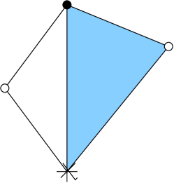
Figure 6: A butterfly

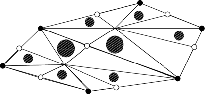
Figure 7: A union of butterflies

We remark that each triangle of this new triangulation has three different vertices : white, black, $*$; each edge is adjacent to a triangle $+$ and a triangle $-$; each face of ${\mathcal{D}}$ is the union of an even number $2p$ of triangles, with $p$ triangles of type $+$ and $p$ triangles of type $-$. Of course, this construction depends on the positions of the center of the faces $f$ and of the shape of the new edges, but we will see that it is not important for our purpose. For further use, following [14], we call butterfly the union of a triangle $t^{+}$ and a triangle $t^{-}$ adjacent at an $(.-*)$-edge of the new triangulation ${\mathcal{T}}$, so that, for instance, triangular face is the union of three butterflies.

Here are two examples :

• Let us consider the unit $2$-sphere $\hbox{\bb S}^{2}$ of $\hbox{\bb E}^{3}$ endowed with its equator. Let $0=(0,0,1)$, $1=(0,1,0)$, $N$ be the north pole and $S$ be the south pole. Let us build the edges $0-1$ and $1-0$ on the equator. This is the simplest dessin on $\hbox{\bb S}^{2}$, with two faces ! Moreover, an associated triangulation is built by adding $N$ and $S$ and drawing curves from $N$ to $0$ and $1$, (resp. $S$ to $0$ and $1$).

• If ${\mathcal{T}}$ is any triangulation on a surface $X$, we color its vertices in black. We add a white vertex in the interior of each edge and a $*$-vertex in the interior of each face, we build a new triangulation by using the construction described in 2 and 3.

10 Building complex structures on a dessin

Our goal now is to define explicit complex structures on a dessin, based on the previous constructions.

• In subsection 10.1, we will associate a first conformal structure ${\mathcal{C}}_{1}$ to a topological surface $x$ endowed with a dessin ${\mathcal{D}}$.

• In subsection 10.2, we will associate to a topological surface $x$ endowed with a dessin ${\mathcal{D}}$ a (in general ramified and not unique) covering map

  $$\beta:X\to\hat{\hbox{\bb C}},$$

  that induces on $X$ a conformal structure ${\mathcal{C}}_{2}$.

• In subsection 10.3, we will compare ${\mathcal{C}}_{1}$ and ${\mathcal{C}}_{2}$.

10.1 Construction of ${\mathcal{C}}_{1}$

Let $(X,{\mathcal{D}})$ be a topological (closed oriented) surface endowed with a dessin. Let ${\mathcal{T}}$ be a triangulation obtained by the construction described in section 9.2. We endow ${\mathcal{T}}$ with the structure of equilateral Euclidean triangulation by affecting the length $1$ to each edge of ${\mathcal{T}}$. We remark that this Riemannian structure is independent of the choice of the position of the vertex added in each face and the ”shape” of the edges of ${\mathcal{T}}$, since two such Euclidean triangulations are isometric by construction. Then, we apply Theorem 23 (or directly Corollary 4) : ${\mathcal{T}}$ and then $X$ is endowed with a conformal structure. We call it ${\mathcal{C}}_{1}$.

10.2 Construction of ${\mathcal{C}}_{2}$

To build a second conformal structure ${\mathcal{C}}_{2}$ on a topological (closed oriented) surface endowed with a dessin, we follow the idea of A. Grothendieck. It needs two steps :

10.2.1 Construction of a (generally) ramified covering over $\hat{\hbox{\bb C}}$

We build a ramified covering

$$\beta:X\to\hat{\hbox{\bb C}}$$

as follows : We begin to build a triangulation ${\mathcal{T}}$ of ${\mathcal{D}}$ by defining butterflies $t^{+}\cup t^{-}$ (see section 9.2), in such a way that ${\mathcal{T}}$ becomes a union of butterflies. Then,

• one builds an homeomorphism from each butterfly $b=t^{+}\cup t^{-}$ to $\hat{\hbox{\bb C}}\simeq\hbox{\bb S}^{2}$, whose equator is identified with $\hbox{\bb R}\cup\infty$. The triangle $t^{+}$ (resp. $t^{-}$) is sent homeomorphically onto the superior (resp. inferior) hemisphere by sending the boundary of $t^{+}$ onto the equator, such that the white vertex is sent to $0$, the black one onto $1$ and the $*$ onto $\infty$. We get an homeomorphism from $b$ to $S^{2}$.

• By building such an homeomorphism for each butterfly, we build a map

  $$\beta:X\to\hat{\hbox{\bb C}}\simeq\hbox{\bb S}^{2},$$

  from $X$ to $\hbox{\bb S}^{2}$, that is locally one-one at each point of $X$ different to the vertices of ${\mathcal{D}}$ : each white vertex is sent onto $0$, each black vertex is sent onto $1$ and each $*$ is sent to $\infty$. Consequently, $\beta$ a covering from $X$ over $S^{2}$, depending on $\mathcal{D}$, ramified at most above the points $0$, $1$ and $\infty$. The degree of this covering is the number of butterflies, the index of ramification of $0$ is the number of white vertices, the index of ramification of $1$ is the number of black vertices, and the index of ramification of $\infty$ is the number of faces of ${\mathcal{D}}$.

10.2.2 Construction of ${\mathcal{C}}_{2}$ by pullback

We will now use a classical result on complex functions :

Proposition 7

Let $X_{1}$ be a topological surface, $X_{2}$ be a Riemann surface,

$$\beta:X_{1}\to X_{2}$$

be a covering of finite degree, ramified at a finite number of points $z_{1},...,z_{k}$ of $X_{1}$. Let $X^{\prime}_{1}=X_{1}\backslash\{z_{1},...,z_{k}\}$. Then,

1. $X^{\prime 1}$ is canonically endowed with the complex structure defined by pulling back by $\beta$ the complex structure of $X_{2}\backslash\{\beta(z_{1}),...,\beta(z_{k})\}$.

2. Moreover, there exists a unique Riemann structure on $X_{1}$ extending the one defined on $X^{\prime 1}$, so that $\beta$ is holomorphic.

Applying Proposition 7, with $X_{1}=X$, $X_{2}=\hat{\hbox{\bb C}}$, $\beta$ the (generally ramified) covering build in the previous paragraph, $k=3$, $\beta(z_{1})=0$, $\beta(z_{2})=1$, $\beta(z_{3})=\infty$, we conclude that a dessin $(X,{\mathcal{D}})$ is endowed with a complex structure. However, it is also clear that this construction depends on $\beta$ and the choice of the vertices $*$ in each face, the shape of the edges $0-*$ and $1-*$ and on the choice a priori to send the white points on $0$ and the black ones on $1$ (we could do the converse). But, modulo an equivalence of covering and a Moebius transformation of $\hat{\hbox{\bb C}}$, this construction is unique. Moreover, by pulling back the complex structure of $\hat{\hbox{\bb C}}$ onto $X$, one endows $X$ with a structure of Riemann surface, and ${\mathcal{T}}$ is the inverse image of the triangle $0,1,\infty$ of $\hat{\hbox{\bb C}}$.

We know (Theorem 11) that any (compact oriented) Riemann surface admits a (generally ramified) covering over ${\hat{\hbox{\bb C}}}$. The construction described in Proposition 7 allows to build on any (compact oriented) topological surface endowed with a dessin, a structure of Riemann surface (endowed with a conformal structure ${\mathcal{C}}_{2}$) and a particular (generally ramified) covering over $\hat{\hbox{\bb C}}$ that is holomorphic. Such a covering ramifies at most over three points. This leads to introduce the following definition :

Definition 7

Let $X$ be a compact Riemann surface. A non constant meromorphic function

$$\beta:X\to\hat{\hbox{\bb C}},$$

is a Belyi function if it ramifies at most above three points. In this case, the couple $(X,\beta)$ is called a Belyi pair.

Usually, via a Moebius transformation of $\hat{\hbox{\bb C}}$, the three points involved in Definition 7 can be systematically taken as $0,1,\infty$.

We deduce the following theorem :

Theorem 25

• A dessin $(X,{\mathcal{D}})$ defined on a topological (compact oriented) surface induces a canonical structure of Riemann surface on $X$ and a Belyi function

  $$\beta:X\to\hat{\hbox{\bb C}}$$

  such that ${\mathcal{D}}=\beta^{-1}([0,1])$.

• Conversely, if

  $$\beta:X\to\hat{\hbox{\bb C}}$$

  is a Belyi function defined on a (compact oriented) Riemann surface, ramified over at most the three points $0,1,\infty$, then ${\mathcal{D}}=\beta^{-1}([0,1])$ is a dessin on $X$.

In Theorem 25, we suppose that the ramification values are $0,1,\infty$. It is not a restriction because, up to a Moebius transformation of $\hat{\hbox{\bb C}}$, we can always (without loss of generality) send the white vertices of ${\mathcal{D}}$ onto $0$ and the black ones onto $1$. On the other hand, we remark that, although the structure of Riemann surface associated to the dessin by mean of a Belyi function is unique, the Belyi function itself is not (it depends in particular on the position of the $*$-vertices of the triangulation and the homeomorphism from each butterfly onto $\hbox{\bb S}^{2}$).

10.3 Coincidence of ${\mathcal{C}}_{1}$ and ${\mathcal{C}}_{2}$ for equilateral triangulations

In this section, we will show that the Riemann structures ${\mathcal{C}}_{1}$ built in section 10.1 and ${\mathcal{C}}_{2}$ built in section 10.2, induced by a dessin $(X,{\mathcal{D}})$ are identical if ${\mathcal{D}}$ is an equilateral triangulation.

Theorem 26

Let $X$ be a (compact oriented) Riemann surface. The following assertions are equivalent :

1. The conformal structure of $X$ is the ${\mathcal{C}}_{2}$-structure associated to the Belyi function obtained from a triangulation ${\mathcal{T}}$ on $X$.

2. The conformal structure of $X$ is the ${\mathcal{C}}_{1}$-structure associated to an equilateral Euclidean triangulation ${\mathcal{T}}$ on $X$.

Proof of Theorem 26 -

1. Let us first suppose that the conformal structure of $X$ is the ${\mathcal{C}}_{2}$-structure associated to a Belyi function

   $$\beta:X\to\hat{\hbox{\bb C}},$$

   constructed from a triangulation ${\mathcal{T}}$ on $X$, whose ramified values belong to $\{0,1,\infty\}$. Let us consider the equilateral Euclidean triangulation ${\mathcal{T}}^{\prime}$ defined on $\hat{\hbox{\bb C}}$ with vertices $\{0,1,\infty\}$. Then, ${\mathcal{T}}=\beta^{-1}{\mathcal{T}}^{\prime}$ can be endowed with a metric such that each of its triangle $t$ is isometric to $\beta(t)$. This metric may have singularities at the vertices of ${\mathcal{T}}$. All triangles of ${\mathcal{T}}$ are isometric, and ${\mathcal{T}}$ is an equilateral Euclidean triangulation on $X$. Let $\{v_{1},...,v_{n}\}$ denotes the set of vertices of ${\mathcal{T}}$. The covering $\beta$ induces a local isometry (and then a locally biholomorphic covering) from $X\backslash\{v_{1},...,v_{n}\}$ onto $\hat{\hbox{\bb C}}\backslash\{0,1,\infty\}$. Consequently, the conformal structure ${\mathcal{C}}_{1}$ of $X\backslash\{v_{1},...,v_{n}\}$ (induced by the equilateral triangulation ${\mathcal{T}}$) coincides with the conformal structure ${\mathcal{C}}_{2}$ on $X\backslash\{v_{1},...,v_{n}\}$ induces by $\beta$. Because $\{v_{1},...,v_{n}\}$ ia a finite set, these structures coincide everywhere on $X$.

2. Conversely, let us suppose that the conformal structure of $X$ is the ${\mathcal{C}}_{1}$-structure associated to an equilateral Euclidean triangulation ${\mathcal{T}}$ on $X$. We will build a Riemann covering of $X$ over $\hat{\hbox{\bb C}}$ as follows :

   

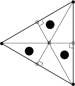
   Figure 8: A butterfly with right triangles

   

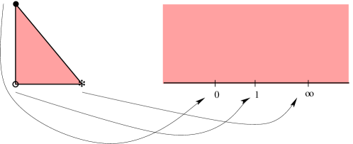
   Figure 9: Sending a right triangle onto $\hbox{\bb C}^{+}$

   

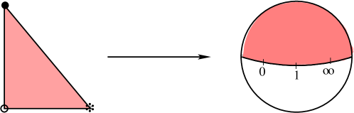
   Figure 10: Sending a right triangle onto the north hemisphere of $S^{2}\simeq\hat{\hbox{\bb C}}$

   • First of all, we will build a ”Euclidean butterfly decomposition” of each triangle $t$ of ${\mathcal{T}}$ by building a new tricolored triangulation $\overline{{\mathcal{T}}}$ as follows : We color the vertices of ${\mathcal{T}}$ in black. By drawing the medians of each triangle $t$, we decompose each triangle of ${\mathcal{T}}$ in $6$ right triangles, coloring in white the vertices that are the intersections of the edges of ${\mathcal{T}}$ with the medians and in $*$ the vertices that are the intersections of the medians. We get for each equilateral triangle $t\in{\mathcal{T}}$, $6$ triangles with angles of $\frac{\pi}{6}$, $\frac{\pi}{3}$, $\frac{\pi}{2}$.

   • Then, we color alternatively each triangle of $\overline{{\mathcal{T}}}$ in black and white, denoting by $t^{+}$ the black ones and by $t^{-}$ the white ones. Each triangle becomes the union of $3$ butterflies $t^{+}\cup t^{-}$. We get $6$ triangles with angles of $30$, $60$, $90$ degrees.

   • Now, we build a biholomorphism from each butterfly onto $\hat{\hbox{\bb C}}$ as follows. Using the Riemann mapping Theorem 8 and the (inverse of) the Riemann Christoffel transformation (Theorem 9), we build a holomorphic transformation $\beta^{+}$ of each triangle $t^{+}$ onto the upper plane $\hat{\hbox{\bb C}}^{+}$, sending the boundary of $t^{+}$ onto the boundary $\overline{\hbox{\bb R}}$, such that the black vertex is send onto $0\in\hbox{\bb R}$, the white vertex onto $1\in\hbox{\bb R}$ and the $*$-vertex onto $\infty$. By the same process, we build a holomorphic transformation $\beta^{-}$ of each triangle $t^{-}$ onto the lower plane $\hat{\hbox{\bb C}}^{-}$. Since $t^{+}$ and $t^{-}$ are isometric, $\beta^{+}$ and $\beta^{-}$ coincide on the common edge of $t^{+}$ and $t^{-}$. We obtain a continuous map $\beta^{\pm}$ from a butterfly onto $\hat{\hbox{\bb C}}$, that is biholomorphic except eventually on the common edge the $t^{+}$ and $t^{-}$. By the reminders of Section 2.2, this transformation is a biholomorphism.

   • We go on, by building a holomorphic covering of degree $3$ from each triangle $t\in{\mathcal{T}}$ over $\hat{\hbox{\bb C}}$

     $$\beta_{t}:t\to\hat{\hbox{\bb C}},$$

     of degree $3$ (ramified over $\infty$), and then, a holomorphic covering

     $$\beta:X\to\hat{\hbox{\bb C}},$$

     (ramified over at most the three points $0,1,\infty$) such that ${\mathcal{T}}=\beta^{-1}([0,1])$.

   Finally, The covering $\beta$ is a Belyi function, $(X,\beta)$ is a Belyi pair, from which we deduce that the conformal structure ${\mathcal{C}}_{2}$ associated to the dessin ${\mathcal{T}}$ via the Belyi function $\beta$ is nothing but ${\mathcal{C}}_{1}$.

11 Automorphisms of a dessin

Classically, an automorphism of graph is a bijection of the set of vertices of the graph preserving the set of edges : a pair of vertices is an edge if and only if its image by the bijection is also an edge. Let us now define an automorphism of a dessin. Although a purely combinatorial definition is possible, we prefer in our context a topological one.

Definition 8

An automorphism of a dessin $(X,{\mathcal{D}})$ is an isotopy class of homeomorphisms of $X$ preserving the graph ${\mathcal{D}}$ and the color of its vertices. We denote by $\mbox{\rm Aut}(X,{\mathcal{D}})$ the group of automorphisms of the dessin $(X,{\mathcal{D}})$.

Of course, two homeomorphisms of $X$ preserving ${\mathcal{D}}$ can induce the same automorphism of the graph ${\mathcal{D}}$. However, one has the following important result [10], [6] :

Proposition 8

In each isotopy class of automorphism of a dessin $(X,{\mathcal{D}})$, there exists a unique (biholomorphic) automorphism of the Riemann surface $X$.

Proof of Proposition 8 - Let ${\mathcal{T}}$ be the equilateral triangulation associated to ${\mathcal{D}}$. There is a unique isometry of $X$ endowed with the Euclidean structure associated to ${\mathcal{T}}$ on $X$, in an isotopy class of homeomorphism of the Riemann surface $X$ (endowed with the ${\mathcal{C}}_{1}={\mathcal{C}}_{2}$-conformal structure - see Theorem 26 -), preserving the graph ${\mathcal{D}}$ and the color of its vertices. This isometry induces a biholomorphic automorphism of $X$ preserving the ${\mathcal{D}}$ and the color of its vertices.

Since ${\rm Aut}(X,{\mathcal{D}})$ is obviously finite, we deduce from Proposition 8, Theorem 14 and Theorem 3 :

Lemma 4

Let $(X,{\mathcal{D}})$ be a dessin. Then, there exists a canonical injective morphism of the group ${\rm Aut}(X,{\mathcal{D}})$ into the group ${\rm Aut}(X)$ of (biholomorphic) automorphisms of $X$, identifying canonically ${\rm Aut}({\mathcal{D}})$ to a finite subgroup of ${\rm Aut}(X)$. In particular, ${\rm Aut}(X,{\mathcal{D}})$ is conjugate to a finite subgroup of $SO(3)$.

12 Proof of Theorem 1

Gathering together Theorem 25, section 7.1, Lemma 4, Proposition 6, Theorem 17, Theorem 22 and Theorem 21, we solve our initial problem : Let $(X,\mathcal{D})$ be a dessin. By section 10, we know that $(X,{\mathcal{D}})$ admits a Belyi function and a canonical complex structure. We will distinguish the cases ${\bf g}_{X}\neq 1$ and ${\bf g}_{X}=0$.

12.1 The case ${\bf g}_{X}\neq 0$

• If ${\bf g}_{X}>1$, $(X,{\mathcal{D}})$ admits a canonical Riemannian metric with constant Gaussian curvature $-1$, that is, the unique metric given by Corollary 22, invariant by the group of biholomorphisms of $X$.

• If ${\bf g}_{X}=1$, $(X,{\mathcal{D}})$ admits, up to a scaling constant, a canonical flat Riemannian metric, that is, the metric given by Theorem 22, invariant by the group of biholomorphisms of $X$.

12.2 The case ${\bf g}_{X}=0$

If ${\bf g}_{X}=0$, by Theorem 17, $X\simeq\hat{\hbox{\bb C}}$ admits a unique structure of Riemann surface, identified with $\hat{\hbox{\bb C}}$. We have seen in section 7.1 that there is no canonical Riemannian metric (invariant under Moebius transformations and of constant Gaussian curvature $1$) associated to this conformal structure. However the data of a dessin d’enfants ${\mathcal{D}}$ induces the data of the subgroup ${\rm Aut}(\hat{\hbox{\bb C}},{\mathcal{D}})$ of ${\rm Aut}(\hat{\hbox{\bb C}})$. That is why, we propose different approaches introducing the automorphism group ${\rm Aut}(\hat{\hbox{\bb C}},{\mathcal{D}})$ to define canonical Riemannian metrics on $\hat{\hbox{\bb C}}$. In each case, we use the fact that ${\rm Aut}(\hat{\hbox{\bb C}},{\mathcal{D}})$ acts on $X$ as a finite subgroup of ${\rm Aut}(\hat{\hbox{\bb C}})$.

1. Our first approach applies directly Proposition 6 : $(\hat{\hbox{\bb C}},{\mathcal{D}})$ can be canonically endowed with the Riemannian metric

   $$\tilde{g}=\frac{1}{{\rm card}({\rm Aut}(\hat{\hbox{\bb C}},{\mathcal{D}}))}\sum_{h\in{\rm Aut}(\hat{\hbox{\bb C}},{\mathcal{D}})}h^{*}(g_{\hat{\hbox{\bb C}}}),$$

   where $g_{\hat{\hbox{\bb C}}}$ is the standard metric of the round sphere of radius $1$. This metric $\tilde{g}$ obviously depends on ${\rm Aut}(\hat{\hbox{\bb C}},{\mathcal{D}})$, and if ${\rm Aut}(\hat{\hbox{\bb C}},{\mathcal{D}})$ is included in $SO(3)$, $\tilde{g}$ coincides with the standard metric $g_{\hat{\hbox{\bb C}}}$ of the round sphere of radius $1$. We remark that the construction of this metric does not requires any restriction on the subgroup ${\rm Aut}(\hat{\hbox{\bb C}},{\mathcal{D}})$. However, the Gaussian curvature of this metric is not constant in general.

2. Our second approach mimics the hyperbolic situation. We know that there exists a unique Riemannian metric of constant curvature $-1$ on ℍ, invariant by the group of biholomorphisms of ${\rm Aut}(\hbox{\bb H})$ (see section 7). Although this strong property is no more true for $\hat{\hbox{\bb C}}$, we will build on $(\hat{\hbox{\bb C}},{\mathcal{D}})$ a Riemannian metric that is invariant by the subgroup ${\rm Aut}(\hat{\hbox{\bb C}},{\mathcal{D}})$ of the group of Moebius transformations ${\rm Aut}(\hat{\hbox{\bb C}})$.

   • Since ${\rm Aut}(\hat{\hbox{\bb C}},{\mathcal{D}})$ is a finite subgroup of $PSL(2,\hbox{\bb C})$ we know by the results of section 1.3 that it is conjugate to a finite subgroup $K$ of $SO(3)$ : there exists $\varphi\in PSL(2,\hbox{\bb C})$ such that

     $${\rm Aut}(\hat{\hbox{\bb C}},{\mathcal{D}})=\varphi^{-1}K\varphi.$$

   • We define the Riemannian metric

     $$g=\phi^{*}g_{\hat{\hbox{\bb C}}},$$

     and we will prove that $g$ does not depend on $\phi$. Suppose that $\psi\in PSL(2,\hbox{\bb C})$ satisfies

     $$\phi^{-1}K\phi=\psi^{-1}K\psi.$$

     then,

     $$\psi\phi^{-1}K\phi\psi^{-1},$$

     that is, $\phi\psi^{-1}$ belongs to the normalizer $N(K)$. We know by Theorem 5 that if $K$ is not cyclic, $N(K)\subset SO(3)$ : There exists $\alpha\in SO(3)$ such that $\psi=\alpha\varphi$. Then,

     $$\psi^{*}g_{\hat{\hbox{\bb C}}}=(\alpha\varphi)^{*}g_{\hat{\hbox{\bb C}}}=\varphi^{*}\alpha^{*}g_{\hat{\hbox{\bb C}}}=\varphi^{*}g_{\hat{\hbox{\bb C}}}.$$

   • Now we prove that $g=\varphi^{*}g_{\hbox{\bb C}}$ is invariant by ${\rm Aut}(\hat{\hbox{\bb C}},{\mathcal{D}})$. As before, we know that there exists a finite subgroup $K$ of $SO(3)$ and $\varphi\in PSL(2,\hbox{\bb C})$ such that

     $${\rm Aut}(\hat{\hbox{\bb C}},{\mathcal{D}})=\varphi^{-1}K\varphi.$$

     Let $\psi\in{\rm Aut}(\hat{\hbox{\bb C}},{\mathcal{D}})$. Let us compare $g$ and $\psi^{*}g$. There exists $\alpha\in K\subset SO(3)$ such that $\psi=\varphi^{-1}\alpha\varphi$. Then,

     $$\psi^{*}g=(\varphi^{-1}\alpha\varphi)^{*}g=\varphi^{*}\alpha^{*}(\varphi^{-1})^{*}\varphi^{*}g_{\hbox{\bb C}}=\varphi^{*}\alpha^{*}g_{\hbox{\bb C}}=\varphi^{*}g_{\hbox{\bb C}}=g.$$

   Finally, $g$ is the solution of our problem.

13 Addendum

We propose here two other constructions of a canonical Riemannian metric on a dessin $(X,{\mathcal{D}})$ when $X$ is a Riemann sphere. In these two last cases, the curvature of the metric is not constant in general.

13.1 Figures of dessins on $\hbox{\bb S}^{2}$ invariant by a finite subgroup of $SO(3)$

Figures 12 and 13 shows the tessellations on $\hbox{\bb S}^{2}$ invariant by $\bf{D}_{n}$ (from Wikipedia, Triangle group) and $\bf{A}_{4}$, $\bf{S}_{4}$, $\bf{A}_{5}$ (from Wikipedia, Triangle group - by Jeff Weeks -).

13.2 A third construction

A third method uses the following proposition :

Proposition 9

Let $K$ be a finite subgroup of ${\rm Aut}(\hat{\hbox{\bb C}})$. Then, $\hbox{\bb C}^{2}$ admits a canonical Hermitian metric $(.,.)_{K}$ invariant by $K$, whose real part $\tilde{\tilde{g}}_{K}$ induces on the Riemann sphere $\hat{\hbox{\bb C}}$ a Riemannian metric that coincide with the metric $g_{\hat{\hbox{\bb C}}}$ of the round sphere if $K$ is a subgroup of $SO(3)$.

Remark that Proposition 9 shows that $K$ is conjugate to a finite subgroup of $SU(2)/\pm 1\simeq SO(3)$.

Proof of Proposition 9 - We consider the sequence of canonical embeddings

$$\hbox{\bb S}^{2}\subset\hbox{\bb C}\times\hbox{\bb R}\subset\hbox{\bb C}\times\hbox{\bb R}^{\hbox{\bb C}}\simeq\hbox{\bb C}\times\hbox{\bb C}=\hbox{\bb C}^{2},$$

where $\hbox{\bb S}^{2}\subset\hbox{\bb C}\times\hbox{\bb R}$ is the standard totally umbilic isometric embedding of the round sphere of radius $1$ in $\hbox{\bb R}^{3}\simeq\hbox{\bb R}^{2}\times\hbox{\bb R}\simeq\hbox{\bb C}\times\hbox{\bb R}$. We deduce the standard isometric embedding

$$\hbox{\bb S}^{2}\to\hbox{\bb S}^{3}\subset\hbox{\bb C}^{2},$$ (8)

where $\hbox{\bb S}^{3}$ is the standard round sphere of radius $1$ in $\hbox{\bb R}^{4}\simeq\hbox{\bb C}^{2}$. Let us take the standard Hermitian scalar product $(.|.)$ on $\hbox{\bb C}^{2}$. If $K$ is any subgroup of ${\rm Aut}(\hat{\hbox{\bb C}})\simeq PSL(2,\hbox{\bb C})$, one can define a new Hermitian scalar product $(.|.)_{K}$ on $\hbox{\bb C}^{2}$ as follows : For all $u$, $v$ in $\hbox{\bb C}^{2}$,

$$(u|v)_{K}=\frac{1}{{\rm card}(K)}\sum_{h\in K}(h(u)|h(v)).$$

(This new Hermitian scalar product is obviously $H$ invariant.) Classically, let us decompose $(.|.)_{K}$ in its real part and its imaginary part :

$$(.|.)_{K}=\tilde{\tilde{g}}_{K}+\imath\Omega_{K},$$

where $\tilde{\tilde{g}}_{K}$ is a Riemannian metric and $\Omega_{K}$ a symplectic form. Using 8, we build on $\hbox{\bb S}^{2}$ the Riemannian metric $\overline{g}_{K}=i^{*}\tilde{\tilde{g}}_{K}$. A priori, $\overline{g}_{K}$ is not a Riemannian metric with constant curvature $1$.

13.3 A fourth construction

Our fourth method uses the study of the orbits of ${\rm Aut}(X,{\mathcal{D}})$, using the classification of the subgroups of $PSL(2,\hbox{\bb C})$ and its consequence : If ${\rm Aut}(X,{\mathcal{D}})$ is not isomorphic to $\hbox{\bb Z}_{n}$, it contains exactly $3$ orbits $O_{1},O_{2},O_{3}$.

• If ${\rm card(O_{1})}<{\rm card(O_{2})}<{\rm card(O_{3})}$, we associate to each triplet $(a_{1},a_{2},a_{3})\in O_{1}\times O_{2}\times O_{3}$, the unique Moebius transformation $h_{a_{1}a_{2}a_{3}}$ that sends $0$ to $a_{1}$, $1$ to $a_{2}$ and $2$ to $a_{3}$. Then, we build the metric

  $$g=\frac{1}{{\rm card}\{a_{1}a_{2}a_{3}\}}\sum_{a_{1}a_{2}a_{3}}h^{*}_{a_{1}a_{2}a_{3}}g_{\hat{\hbox{\bb C}}},$$

  where the sum is over all possible triplets $a_{1}a_{2}a_{3}$ built as before.

• If ${\rm card(O_{1})}={\rm card(O_{2})}<{\rm card(O_{3})}$ (it is the dihedral situation), we cannot distinguish the orbits with the same cardinality, so with the same notations, we associate to each triplet $(a_{1},a_{2},a_{3})\in O_{1}\times O_{2}\times O_{3}$, the unique Moebius transformation $h_{a_{1}a_{2}a_{3}}$ that sends $0$ to $a_{1}$, $1$ to $a_{2}$ and $2$ to $a_{3}$, and the unique Moebius transformation $k_{a_{1}a_{2}a_{3}}$ that sends $0$ to $a_{2}$, $1$ to $a_{1}$ and $2$ to $a_{3}$, . Then we build the metric

  $$g=\frac{1}{2{\rm card}\{a_{1}a_{2}a_{3}\}}\sum_{a_{1}a_{2}a_{3}}h^{*}_{a_{1}a_{2}a_{3}}g_{\hat{\hbox{\bb C}}}+\frac{1}{2{\rm card}\{a_{1}a_{2}a_{3}\}}\sum_{a_{1}a_{2}a_{3}}k^{*}_{a_{1}a_{2}a_{3}}g_{\hat{\hbox{\bb C}}}.$$

• If ${\rm card(O_{1})}<{\rm card(O_{2})}={\rm card(O_{3})}$ (it is the tetrahedral situation), an analogous process builds a canonical metric.

Finally, if ${\rm Aut}(X,{\mathcal{D}})$ is isomorphic to $\hbox{\bb Z}_{n}$, we can arbitrarily endow $\hat{\hbox{\bb C}}$ with the standard metric $g_{\hbox{\bb C}}$.

The reader can produce other Riemannian metrics of this type on $\hat{\hbox{\bb C}}$, playing for instance with the fixed points of the elements of ${\rm Aut}(X,{\mathcal{D}})$.

Figure 12: Tesselations of the $2$-sphere, induced by the action of the diedral group ${\bf D}_{6}$, (From Wikipedia, Triangle group)

Figure 13: Tesselations of the $2$-sphere, induced by the actions of ${\mathcal{A}}_{4}$, ${\mathcal{S}}_{4}$, ${\mathcal{A}}_{5}$, (From Wikipedia, Triangle group)

Jean-Marie Morvan, Université de Lyon, CNRS UMR $5208$, Université Claude Bernard Lyon $1$, Institut Camille Jordan, $43$ blvd du $11$ Novembre $1918$, $F$-$69622$ Villeurbanne-Cedex, France and King Abdullah University of Science and Technology, $C.E.M.S.E$, Thuwal $23955$-$6900$, Saudi Arabia

E-mail address : morvan@math.univ-lyon1.fr and Jean-Marie.Morvan@KAUST.EDU.SA

References

- [1] J.-B. Bost. Introduction to compact Riemann surfaces, Jacobians, and Abelian varieties. From number theory to physics, pp. . Springer, .
- [2] I. Cheltsov and C. Shramov. Cremona groups and the icosahedron. Monographs and Research Notes in Mathematics, , CRC Press.
- [3] J. Dai and X. D. Gu and F. Luo. Variational principles for discrete surfaces. Volume , , International Press of Boston Incorporated.
- [4] S. Donaldson. Riemann surfaces. . Oxford University Press.
- [5] R. Earp and E. Toubiana. Introduction a la geométrie hyperbolique et aux surfaces de Riemann. . Diderot éditeur arts et sciences.
- [6] E. Girondo and G. González-Diez. Introduction to compact Riemann surfaces and dessins d’enfants, Volume , . Cambridge University Press.
- [7] A. Grothendieck. Esquisse d’un programme. Preprint, Montpellier, .
- [8] X. D. Gu and S.T. Yau. Computational conformal geometry. , International Press Somerville, Mass, USA.
- [9] C. Guillarmou and S. Moroianu. Unpublished, web site of C. Guillarmou.
- [10] G. Jones, A. Gareth and J. Wolfart. Dessins d’enfants on Riemann surfaces. , Springer.
- [11] S.K. Lando and A. K. Zvonkin. Graphs on surfaces and their applications. Volume , , Springer Science, Business Media
- [12] J. Malgoire and C. Voisin. Cartes cellulaires. Cahiers Math. Montpellier, volume .
- [13] E. Reyssat Quelques aspects des surfaces de Riemann. , Progress in Math. , Birkhauser.
- [14] G. B. Shabat and V.A. Voevodsky. title=Drawing curves over number fields. The Grothendieck Festschrift, , , Springer.
- [15] Ch. Voisin and J. Malgoire. Cartes topologiques infinies et revêtements ramifiés de la sphère. , Univ. des Sciences et Techniques du Languedoc, UER de Mathématiques.