$C^{\infty}$-convergence of conformal mappings for conformally equivalent triangular lattices

Abstract.

Two triangle meshes are conformally equivalent if for any pair of incident triangles the absolute values of the corresponding cross-ratios of the four vertices agree. Such a pair can be considered as preimage and image of a discrete conformal map. In this article we study discrete conformal maps which are defined on parts of a triangular lattice $T$ with strictly acute angles. That is, $T$ is an infinite triangulation of the plane with congruent strictly acute triangles. A smooth conformal map $f$ can be approximated on a compact subset by such discrete conformal maps $f^{\varepsilon}$, defined on a part of $\varepsilon T$, see [Büc16]. We improve this result and show that the convergence is in fact in $C^{\infty}$. Furthermore, we describe how the cross-ratios of the four vertices for pairs of incident triangles are related to the Schwarzian derivative of $f$.

1. Introduction

Holomorphic functions build the basis and heart of the rich theory of complex analysis. The subclass of conformal maps consists of holomorphic functions with nowhere vanishing derivatives. These may be characterized as infinitesimal scale-rotations. Möbius transformations are special conformal maps on the Riemann sphere $\hat{\mathbb{C}}$, which preserve all cross-ratios. Recall that the cross-ratio of four distinct points $a,b,c,d\in\mathbb{C}$ is defined as

$$\mathrm{cr}(a,b,c,d)=\frac{(a-b)(c-d)}{(b-c)(d-a)}.$$

A conformal map $f$ infinitesimally preserves cross-ratios. Additionally, the first deviation from being a Möbius transformation can be expressed by the Schwarzian derivative of $f$, which is defined as

$${\mathfrak{S}}[f](z)=\left(\frac{f^{\prime\prime}(z)}{f^{\prime}(z)}\right)^{\prime}-\frac{1}{2}\left(\frac{f^{\prime\prime}(z)}{f^{\prime}(z)}\right)^{2}=\frac{f^{\prime\prime\prime}(z)}{f^{\prime}(z)}-\frac{3}{2}\left(\frac{f^{\prime\prime}(z)}{f^{\prime}(z)}\right)^{2}.$$ (1)

In particular, there holds

$$\lim_{\varepsilon\to 0}\frac{1}{\varepsilon^{2}}\left(\frac{\mathrm{cr}(f(a),f(a+\varepsilon(b-a)),f(a+\varepsilon(c-a)),f(a+\varepsilon(d-a)))}{\mathrm{cr}(a,b,c,d)}-1\right)\\ =\frac{(a-c)(b-d)}{6}{\mathfrak{S}}[f](a).$$

1.1. $C^{\infty}$-convergence for discrete conformal maps on triangular lattices

In the discrete theory, the idea of characterizing conformal maps as local scale-rotations may be translated into different concepts. Here we consider the discretization coming from a metric viewpoint: Infinitesimally, lengths are scaled by a factor, i.e. by $|f^{\prime}(z)|$ for a conformal function $f$ on $D\subset\mathbb{C}$. The smooth complex domain is replaced in this discrete setting by a triangulation of a connected subset of the plane $\mathbb{C}$. The infinitesimal preservation of the cross-ratios is then substituted by the preservation of all length cross-ratios ($=$ absolute values of the cross-ratio) for all pairs of incident triangles. (Note that only Möbius transformations would preserve all cross-ratios of pairs of incident triangles of the triangulation. So this condition would be two restrictive.)

In this article we consider the case where the triangulation is a (part of a) triangular lattice. In particular, let $T$ be a lattice triangulation of the whole complex plane $\mathbb{C}$ with congruent triangles, see Figure 1(a).

(a) Example of a triangular lattice.

(b) Suitably scaled acute angled triangle.

Figure 1. Lattice triangulation of the plane with congruent triangles.

The sets of vertices and edges of $T$ are denoted by $V$ and $E$ respectively. Edges will often be written as $e=[v_{i},v_{j}]\in E$, where $v_{i},v_{j}\in V$ are its incident vertices. For triangular faces we use the notation $\Delta[v_{i},v_{j},v_{k}]$ enumerating the incident vertices with respect to the orientation (counterclockwise) of $\mathbb{C}$. We only consider the case of acute angles, i.e., $\alpha,\beta,\gamma\in(0,\pi/2)$ and assume for simplicity that the origin is a vertex.

On a subcomplex of $T$ we now define a discrete conformal mapping by the preservation of the length cross-ratios.

Definition 1.1 (see [BPS15]).

A discrete conformal map $g$ is the restriction to the vertices $V_{S}$ of a continuous and orientation preserving map $g_{\text{PL}}$ of a subcomplex $T_{S}$ of a triangular lattice $T$ to $\mathbb{C}$. We demand that $g_{\text{PL}}$ is locally a homeomorphism in a neighborhood of each interior point and that its restriction to every triangle is a linear map onto the corresponding image triangle, that is the mapping is piecewise linear. Furthermore, the absolute value of the cross-ratio (called length cross-ratio) is preserved for all pairs of adjacent triangles:

$$|\mathrm{cr}(v_{1},v_{2},v_{3},v_{4})|=|\mathrm{cr}(g(v_{1}),g(v_{2}),g(v_{3}),g(v_{4}))|,$$ (2)

where $\Delta[v_{1},v_{2},v_{3}]$ and $\Delta[v_{1},v_{3},v_{4}]$ are two adjacent triangles of the lattice with common edge $[v_{1},v_{3}]$ and $|a|$ denotes the modulus of $a\in\mathbb{C}$.

Note that the values of the cross-ratio $\mathrm{cr}(g(v_{1}),g(v_{2}),g(v_{3}),g(v_{4}))$ on all interior edges $[v_{1},v_{3}]$ determine the map $g$ up to a global Möbius transformation, see also Remark 3.2 below for more details.

Remark 1.2 ([BPS15]).

For a continuous, orientation preserving and piecewise linear map $g_{\text{PL}}$ on a simply connected subcomplex the preservation of the length cross-ratios is equivalent to the existence of a function $u:V_{S}\to\mathbb{R}$ on the vertices, called associated scale factors, such that for all edges $e=[v,w]\in E_{S}$ there holds

$$|g(v)-g(w)|=|v-w|\text{e}^{(u(v)+u(w))/2}.$$ (3)

Thus the lengths of the edges of the triangulation are changed according to scale factors at the vertices. The new triangles are then “glued together” to result in a piecewise linear map, see Figure 2 for an illustration.

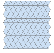
$$\overset{g}{\longrightarrow}$$

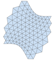
Figure 2. Example of a discrete conformal map $g$.

In fact, our definition of a discrete conformal map relies on the notion of discretely conformally equivalent triangle meshes. These have been studied by Luo, Gu, Sun, Wu, Guo [Luo04, GLSW, GGL⁺], Bobenko, Pinkall, and Springborn [BPS15] and others.

In [Büc16] we showed that given a smooth conformal map $f$ there exists a sequence of discrete conformal maps $f^{\varepsilon}$ which approximates the given map on a compact set. In particular, the discrete conformal maps can be obtained from a Dirichlet problem: Given some function $u_{\partial}$ on the boundary of a subcomplex $T_{S}$, find a discrete conformal map whose associated scale factors agree on the boundary with $u_{\partial}$. Of course, we choose the boundary values $u_{\partial}$ according to the given function $f$ as $u_{\partial}=\log|f^{\prime}|$. In this article we improve this result and show that the approximation in fact is $C^{\infty}$. Furthermore, as a by-product, we establish the approximation of the Schwarzian derivative of $f$ using cross-ratios of pairs of incident triangles.

To be precise, denote by $\varepsilon T$ the lattice $T$ scaled by $\varepsilon>0$.

Theorem 1.3 ([Büc16, Theorem 1.1]).

Let $f:D\to\mathbb{C}$ be a conformal map (i.e. holomorphic with $f^{\prime}\not=0$). Let $K\subset D$ be a compact set which is the closure of its simply connected interior $\Omega_{K}:=int(K)$ and assume that $0\in\Omega_{K}$. Let $T$ be a triangular lattice with strictly acute angles. For each $\varepsilon>0$ let $T^{\varepsilon}_{K}$ be a subcomplex of $\varepsilon T$ whose support is contained in $K$ and is homeomorphic to a closed disc. We further assume that $0$ is an interior vertex of $T^{\varepsilon}_{K}$. Let $e_{0}=[0,{\mathbb{v}_{\mathbb{0}}}]\in E^{\varepsilon}_{K}$ be one of its incident edges.

Then if $\varepsilon>0$ is small enough (depending on $K$, $f$, and $T$) there exists a unique discrete conformal map $f^{\varepsilon}$ on $T^{\varepsilon}_{K}$ which satisfies the following two conditions:

• The associated scale factors $u^{\varepsilon}:V^{\varepsilon}_{K}\to\mathbb{R}$ satisfy

  $$u^{\varepsilon}(v)=\log|f^{\prime}(v)|\qquad\text{for all boundary vertices }v\text{ of }V^{\varepsilon}_{K}.$$ (4)

• The discrete conformal map is normalized according to

  $$\qquad f^{\varepsilon}(0)=f(0)\quad\text{and}\quad\arg(f^{\varepsilon}({\mathbb{v}_{\mathbb{0}}})-f^{\varepsilon}(0))=\arg({\mathbb{v}_{\mathbb{0}}})+\arg(f^{\prime}(\frac{{\mathbb{v}_{\mathbb{0}}}}{2}))\pmod{2\pi}.$$

Furthermore, the following estimates for $u^{\varepsilon}$ and $f^{\varepsilon}$ hold for all vertices $v\in V^{\varepsilon}_{K}$ and points $x$ in the support of $T^{\varepsilon}_{K}$ respectively with constants $C_{1},C_{2}$ depending only on $K$, $f$, and $T$, but not on $v$ or $x$:

1. The scale factors $u^{\varepsilon}$ approximate $\log|f^{\prime}|$ uniformly with error of order $\varepsilon^{2}$:

   $$\left|u^{\varepsilon}(v)-\log|f^{\prime}(v)|\right|\leq C_{1}\varepsilon^{2}.$$ (5)

2. The discrete conformal maps $f^{\varepsilon}$ converge to $f$ for $\varepsilon\to 0$ uniformly with error of order $\varepsilon$:

   $$\left|f^{\varepsilon}_{\text{PL}}(x)-f(x)\right|\leq C_{2}\varepsilon,$$

   where $f^{\varepsilon}_{\text{PL}}$ is the piecewise linear extension of $f^{\varepsilon}$ from Definition 1.1.

In this article the subcomplexes $T^{\varepsilon}_{K}$ will be chosen such that they approximate the compact set $K$. In particular, we will take for $T^{\varepsilon}_{K}$ a subcomplex which is simply connected, contained in $K$ and contains $0$ and is “as large as possible”. This means in particular, that adding any other triangle of $\varepsilon T$ which is contained in $K$ and shares an edge with a triangle of $T^{\varepsilon}_{K}$ will result in a subcomplex which ceases to be simply connected.

Theorem 1.4.

Under the assumptions of Theorem 1.3 and with the above definition of $T^{\varepsilon}_{K}$, the discrete conformal maps converges in $C^{\infty}(\Omega)$ to $f$.

The proof of Theorem 1.4 is inspired by the methods of the proof of $C^{\infty}$-convergence for hexagonal circle packings in [HS98]. In particular, the main objects are discrete Schwarzians defined in Section 3 as suitably scaled measure of deformation of the Möbius invariant cross-ratios from their original values in the lattice $T$. As the discrete Laplacian of such a discrete Schwarzian is a polynomial in $\varepsilon$ and the discrete Schwarzians, we can deduce their $C^{\infty}$-convergence in Section 4 analogously as in [HS98] from a Regularity lemma 4.2 using some facts on discrete differential operators introduced in Section 2. The necessary boundedness of the discrete Schwarzian itself can be deduced from Theorem 1.3. Finally, the $C^{\infty}$-convergence of $f^{\varepsilon}$ is shown in Section 5. Here, we also derive the precise connection between the limits of the discrete Schwarzians and the Schwarzian derivative of the given function $f$. In Section 6 we discuss some generalizations of our proof, for example to the convergence of circle patterns with hexagonal combinatorics and other notions of discrete conformality.

1.2. Other convergence results for discrete conformal maps

Smooth conformal maps can be characterized in various ways. This leads to different notions of discrete conformality. Convergence issues have already been studied for some of these discrete analogs. We only give a very short overview and cite some results of a growing literature.

Linear definitions can be derived as discrete versions of the Cauchy-Riemann equations and have a long and still developing history. Connections of such discrete mappings to smooth conformal functions have been studied for example in [CFL28, LF55, Mer07, CS12, Sko13, BS16, Wer14]. In particular, this includes $C^{\infty}$-convergence for the regular $\varepsilon\mathbb{Z}^{2}$-lattice.

The idea of characterizing conformal maps as local scale-rotations has lead to the consideration of circle packings, more precisely to investigations on circle packings with the same (given) combinatorics of the tangency graph. Thurston [Thu85] first conjectured the convergence of circle packings to the Riemann map, which was then proven by [RS87, HS96, Ste97]. $C^{\infty}$-convergence for hexagonal circle packings was shown in [HS98].

The theory of circle patterns generalizes the case of circle packings. Also, there is a link to integrable structures via isoradial circle patterns. The approximation of conformal maps using circle pattens has been studied in [Sch97] for orthogonal circle patterns with square grid combinatorics and furthermore in [Mat05, Büc07, Büc08, LD07, BBS17], which also contain results on $C^{\infty}$-convergence.

2. Preliminaries on discrete differential operators and notation

In the following, we introduce useful definitions and notation by generalizing the notions defined in [HS98, Sec. 2].

We consider the regular triangular lattice $\varepsilon T$ with edge length $\varepsilon>0$. In particular, let

$$V^{\varepsilon}=\{n\varepsilon\sin\alpha+m\text{e}^{i\beta}\varepsilon\sin\gamma:n,m\in\mathbb{Z}\}$$

be the set of vertices. We abbreviate the edge directions by

$$\omega_{1}=1=-\omega_{4},\qquad\omega_{2}=\text{e}^{i\beta}=-\omega_{5},\qquad\omega_{3}=\text{e}^{i(\alpha+\beta)}=-\omega_{6},$$

and the corresponding edge lengths in $T$ as in Figure 1(b) by

$$L_{1}=\sin\alpha=L_{4},\qquad L_{2}=\sin\gamma=L_{5},\qquad L_{3}=\sin\beta=L_{6}.$$

Note in particular, that $L_{1}\omega_{1}-L_{2}\omega_{2}+L_{3}\omega_{3}=0$.

For $k=1,\dots,6$ denote by $\tau^{\varepsilon}_{k}:V^{\varepsilon}\to V^{\varepsilon}$, $\tau^{\varepsilon}_{k}v=v+\varepsilon L_{k}\omega_{k}$ the translation along one of the lattice directions. For any subset $W\subseteq V^{\varepsilon}$ a vertex $v\in W$ is called interior vertex of $W$ if all neighboring vertices $\tau^{\varepsilon}_{k}v$ for $k=1,\dots,6$ are contained in $W$. Set $W^{(0)}=W$ and for each $l\geq 1$ denote by $W^{(l)}$ the set of interior vertices of $W^{(l-1)}$.

Given a function $\eta:W\to\mathbb{C}$, denote by $\tau_{k}^{\varepsilon}\eta$ the function which differs from $\eta$ by a translation $\tau_{k}^{\varepsilon}$:

$$\tau_{k}^{\varepsilon}\eta(v)=\eta(\tau_{k}^{\varepsilon}v)=\eta(v+\varepsilon L_{k}\omega_{k}).$$

Define the (discrete) directional derivative $\partial_{k}^{\varepsilon}\eta:W^{(1)}\to\mathbb{R}$ by

$$\partial_{k}^{\varepsilon}\eta(v)=\frac{1}{\varepsilon L_{k}}(\eta(v+\varepsilon L_{k}\omega_{k})-\eta(v)),$$

so $\partial_{k}^{\varepsilon}=(\varepsilon L_{k})^{-1}(\tau^{\varepsilon}_{k}-I)$, where $I\eta=\eta$. For further use, note the following rule for the discrete differentiation of a product:

$$\partial_{k}^{\varepsilon}(\eta_{1}\eta_{2})=(\partial_{k}^{\varepsilon}\eta_{1})\eta_{2}+\tau_{k}^{\varepsilon}\eta_{1}(\partial_{k}^{\varepsilon}\eta_{2}).$$ (6)

Furthermore, define the (discrete) Laplacian $\Delta^{\varepsilon}\eta:W^{(1)}\to\mathbb{C}$ by

$$\Delta^{\varepsilon}\eta(v)=\frac{1}{\varepsilon^{2}}\sum\limits_{k=1}^{6}i\frac{\omega_{k}^{2}+1}{\omega_{k}^{2}-1}(\eta(v+\varepsilon L_{k}\omega_{k})-\eta(v)).$$ (7)

Note that this is a scaled version of the well-known $\cot$-Laplacian as $\cot\varphi=i(\text{e}^{2i\varphi}+1)/(\text{e}^{2i\varphi}-1)$. Of course, the operators $I$, $\tau_{k}^{\varepsilon}$, $\partial^{\varepsilon}_{j}$ and $\Delta^{\varepsilon}$ commute with each other. We will also use $\|\eta\|_{W}=\sup_{v\in W}|\eta(v)|$ to denote the $L^{\infty}(W)$-norm of $\eta$.

Let $\Omega\subset\mathbb{C}$ be some domain and let $f:\Omega\to\mathbb{C}$ be some function. For each $\varepsilon>0$, let $f^{\varepsilon}:W^{\varepsilon}\to\mathbb{C}$ be some function defined on a set of vertices $W^{\varepsilon}\subset V^{\varepsilon}$. Assume that for every $z\in\Omega$ there are some $\delta_{1},\delta_{2}>0$ such that for all $\varepsilon\in(0,\delta_{1})$ we have $\{v\in V^{\varepsilon}:|v-z|<\delta_{2}\}\subset W^{\varepsilon}$.

Then we say that $f^{\varepsilon}$ converges to $f$ locally uniformly in $\Omega$, if for every $\sigma>0$ and every $z\in\Omega$ there are $\delta_{1},\delta_{2}>0$ such that $|f(z)-f^{\varepsilon}(v)|<\sigma$ for every $\varepsilon\in(0,\delta_{1})$ and every $v\in W^{\varepsilon}$ with $|v-z|<\delta_{2}$.

If $f$ is differentiable, denote by $\partial_{k}f$ the directional derivative, that is

$$\partial_{k}f(z)=\lim\limits_{t\to 0}\frac{f(z+t\omega_{k})-f(z)}{t}\qquad\text{ for }k=1,\dots,6.$$

Let $n\in\mathbb{N}$ and suppose that $f$ is $C^{n}$-smooth. We call $f^{\varepsilon}$ convergent to $f$ in $C^{n}(\Omega)$ if for every sequence $k_{1},\dots,k_{j}\in\{1,\dots,6\}$ with $j\leq n$ the functions $\partial^{\varepsilon}_{k_{j}}\partial^{\varepsilon}_{k_{j-1}}\dots\partial^{\varepsilon}_{k_{1}}f^{\varepsilon}$ converges to $\partial_{k_{j}}\partial_{k_{j-1}}\dots\partial_{k_{1}}f$ locally uniformly in $\Omega$. If this holds for all $n\in\mathbb{N}$, the convergence is $C^{\infty}(\Omega)$.

The functions $f^{\varepsilon}$ are called uniformly bounded in $C^{n}(\Omega)$, if for every compact set ${\cal K}\subset\Omega$ there is some constant $C({\cal K},n)$ such that $\|\partial^{\varepsilon}_{k_{j}}\partial^{\varepsilon}_{k_{j-1}}\dots\partial^{\varepsilon}_{k_{1}}f^{\varepsilon}\|_{W^{\varepsilon}}<C(K,n)$ holds for every $j\leq n$ and all $\varepsilon$ small enough. The functions $f^{\varepsilon}$ are uniformly bounded in $C^{\infty}(\Omega)$ if they are uniformly bounded in $C^{n}(\Omega)$ for all $n\in\mathbb{N}$.

The proofs of the following lemmas are simple adaptions of the corresponding arguments in [HS98, Sect. 2].

Lemma 2.1 (see [HS98, Lemma 2.1]).

Let $n\in\mathbb{N}$. Suppose that the functions $f^{\varepsilon}$ are uniformly bounded in $C^{n+1}(\Omega)$. Then for every sequence $\varepsilon\to 0$ there is a $C^{n}(\Omega)$-function $f$ and a subsequence of $\varepsilon\to 0$ such that $f^{\varepsilon}\to f$ in $C^{n}(\Omega)$ along this subsequence.

Lemma 2.2 (see [HS98, Lemma 2.2]).

Suppose that $f^{\varepsilon},g^{\varepsilon},h^{\varepsilon}$ converges in $C^{\infty}(\Omega)$ to functions $f,g,h:\Omega\to\mathbb{C}$, defined on a domain $\Omega\supset K$, and suppose that $h\not=0$ in $\Omega$. Then the following convergences are in $C^{\infty}(\Omega)$:

1. $f^{\varepsilon}+g^{\varepsilon}\to f+g$,

2. $f^{\varepsilon}g^{\varepsilon}\to fg$,

3. $1/h^{\varepsilon}\to 1/h$,

4. if $h^{\varepsilon}>0$ then $\sqrt{h^{\varepsilon}}\to\sqrt{h}$,

5. $|h^{\varepsilon}|\to|h|$.

3. The discrete Schwarzians

Let $f$ be a conformal map on a domain in the complex plane $\mathbb{C}$, that is, $f$ is a holomorphic function with non-vanishing derivative $f^{\prime}(z)\not=0$. The Schwarzian derivative of $f$ is defined in (1) and is itself holomorphic. Further, for any Möbius transformation $M(z)=(az+b)/(cz+d)$ we have ${\mathfrak{S}}[M\circ f]={\mathfrak{S}}[f]$ and ${\mathfrak{S}}[f]=0$ if and only if $f$ is the restriction of some Möbius transformation. For proofs and further properties of the Schwarzian see for example [Let87, Chap. II].

In the following, we will define Möbius invariants of conformally equivalent triangular lattices and derive their equations. Suitable Möbius invariants and corresponding equations have been worked out in [Sch97] for orthogonal circle patterns and in [HS98] for hexagonal circle packings.

Inspired by [HS98], we will use the Möbius invariants as intermediate means in the study of the convergence problem. The discrete Schwarzians will be defined as suitably scaled measure of deformation of the Möbius invariants from their regular values. The convergence of the discrete Schwarzians is also notable on its own right and increases the connection between analogous notions for smooth and discrete conformal maps.

For any interior edge $[u,v]$ in $T^{\varepsilon}_{K}$ with two adjacent triangles $\Delta[u,v,w_{1}]$ and $\Delta[u,w_{2},v]$ denote by

$$Q([u,v]) =\mathrm{cr}(u,w_{2},v,w_{1}),$$ (8)

$$q^{\varepsilon}([u,v]) =\mathrm{cr}(f^{\varepsilon}(u),f^{\varepsilon}(w_{2}),f^{\varepsilon}(v),f^{\varepsilon}(w_{1}))$$ (9)

the cross-ratio of the four vertices on the quad formed by the the two triangles $\Delta[u,v,w_{1}]$ and $\Delta[u,w_{2},v]$ and by their images under $f^{\varepsilon}$ respectively. Note that $Q([v,v+\varepsilon L_{k}\omega_{k}])=(\omega_{k-1}L_{k-1})^{2}/(\omega_{k+1}L_{k+1})^{2}$ where the indices are taken modulo $6$.

We define the discrete Schwarzian at $[u,v]$ by

$$s([u,v])=\frac{1}{\varepsilon^{2}}\left(\frac{q^{\varepsilon}([u,v])}{Q([u,v])}-1\right).$$ (10)

If $f^{\varepsilon}$ is a Möbius transformation, we have $s([u,v])=0$, analogously to the smooth case.

For any vertex $v\in V^{\varepsilon}$ denote $e_{k}(v)=[v,\tau_{k}^{\varepsilon}(v)]$, see Figure 3 (left). Let $q_{k},s_{k}:(W^{\varepsilon})^{(1)}\to\mathbb{C}$ be defined as $q_{k}(v):=q^{\varepsilon}(e_{k}(v))$ and $s_{k}(v):=s(e_{k}(v))$. Then obviously, $q_{k+3}(\tau_{k}^{\varepsilon}v)=q_{k}(v)$ and

$$s_{k+3}(\tau_{k}^{\varepsilon}v)=s_{k}(v),$$ (11)

where the indices are taken modulo $6$. Note that $Q_{k}:=Q(e_{k}(v))=Q_{k+3}$, as $\varepsilon T$ is a lattice.

Lemma 3.1.

Let $v$ be an interior vertex in $V_{K}^{\varepsilon}$. Then there holds

$$q_{1}(v)q_{2}(v)q_{3}(v)q_{4}(v)q_{5}(v)q_{6}(v)=1$$ (12)

$$1-q_{k}(v)+q_{k}(v)q_{k+1}(v)-q_{k}(v)q_{k+1}(v)q_{k+2}(v)$$

$$\qquad+q_{k}(v)q_{k+1}(v)q_{k+2}(v)q_{k+3}(v)-q_{k}(v)q_{k+1}(v)q_{k+2}(v)q_{k+3}(v)q_{k+4}(v)=0$$ (13)

$$1-{\scriptstyle\frac{1}{|Q_{k}|^{2}}}q_{k}(v)+{\scriptstyle\frac{1}{|Q_{k}|^{2}|Q_{k-1}|^{2}}}q_{k}(v)q_{k-1}(v)-q_{k}(v)q_{k-1}(v)q_{k-2}(v)$$

$$\ +{\scriptstyle\frac{1}{|Q_{k}|^{2}}}q_{k}(v)q_{k-1}(v)q_{k-2}(v)q_{k-3}(v)-{\scriptstyle\frac{1}{|Q_{k}|^{2}|Q_{k-1}|^{2}}}q_{k}(v)q_{k-1}(v)q_{k-2}(v)q_{k-3}(v)q_{k-4}(v)=0$$ (14)

for $k=1,\dots,6$, where the indices are taken modulo $6$, and $|Q_{k}|=L_{k-1}^{2}/L_{k+1}^{2}$.

Remark 3.2.

If the values of a function $q^{\varepsilon}$ all lie in the upper half-plane $\{z\in\mathbb{C}:\text{Im}(z)>0\}$ and $\sum_{k=1}^{6}\arg(q_{k}(v))=4\pi$ holds for all interior vertices $v$, then equations (13)–(14) guarantee that $q^{\varepsilon}$ corresponds to a discrete conformal map on (a part of) a triangular lattice $T_{S}$. Indeed, start with any triangle of $T_{S}$ and map it to any triangle in $\mathbb{C}$ respecting orientation. This defines the values of the discrete conformal map $g$ on the first triangle. Then the values of $g$ on all incident triangles can now be uniquely determined using (9). Our additional assumptions on $q^{\varepsilon}$ show that the pattern is immersed. If $T_{S}$ is the triangulation of a simply connected domain, this procedure subsequently defines $g$ on all vertices. Equations (12)–(14) guarantee that no ambiguities will occur.

Proof of Lemma 3.1..

First note that (12) is an easy consequence of the fact that $q_{k}$ are cross-ratios of a flower. Furthermore, (14) follows from (12) and (13) by taking the complex conjugation of (13) because $|q_{k}(v)|=|Q_{k}|$ using (3).

In order to see (13), add circumcircles to the triangles of the flower around $v_{0}$ and map $v_{0}$ to $\infty$ by a Möbius transformation as illustrated in Figure 3 (right).

Figure 3. Left: A flower about $v$ in the lattice $\varepsilon T$. Right: Mapping the circumcircles of a flower by a Möbius transformation with $v_{0}\mapsto\infty$.

As the Möbius transformation does not change the values of the $q_{k}$’s, we easily identify equations (12) and (13) as the closing conditions for the image polygon. ∎

Our next goal is to derive from (12)–(14) an expression for the Laplacian of the discrete Schwarzians $\Delta^{\varepsilon}s_{k}(v)$ which equals a polynomial in $\varepsilon,s_{j}(v),\tau_{l}s_{m}(v)$ for $j,l,m\in\{1,\dots,6\}$. Then, if all discrete Schwarzians $s_{k}$ are uniformly bounded for small $\varepsilon\in(0,\varepsilon_{0})$ and on $V_{K}^{\varepsilon}$, also all Laplacians $\Delta^{\varepsilon}s_{k}(v)$ are uniformly bounded on $(V_{K}^{\varepsilon})^{(1)}$.

For an interior vertex $v$ substitute $q_{k}(v)=Q_{k}(1+\varepsilon^{2}s_{k}(v))$ in (12)–(14), and obtain (using for example a computer algebra program):

$$\sum_{k=1}^{6}s_{k}(v)= \varepsilon^{2}\Phi(v)$$ (15)

$$s_{k}(v)+s_{k+1}(v)+s_{k+2}(v)-Q_{k}(s_{k+1}(v)+s_{k+2}(v)+s_{k+3}(v))\\ +Q_{k}Q_{k+1}(s_{k+2}(v)+s_{k+3}(v)+s_{k+4}(v))=\varepsilon^{2}\Psi_{k}(v)$$ (16)

$$s_{k}(v)+s_{k-1}(v)+s_{k-2}(v)-\frac{1}{\overline{Q_{k}}}(s_{k-1}(v)+s_{k-2}(v)+s_{k-3}(v))\\ +\frac{1}{\overline{Q_{k}}\overline{Q_{k-1}}}(s_{k-2}(v)+s_{k-3}(v)+s_{k-4}(v))=\varepsilon^{2}\Theta_{k}(v)$$ (17)

$$\text{ where }\qquad\qquad\Phi(v)= -\sum_{k=1}^{5}\sum_{l=k+1}^{6}s_{k}(v)s_{l}(v)-\varepsilon^{2}\sum_{\begin{subarray}{c}k_{1},k_{2},k_{3}\in\{1,\dots,6\}\\ k_{1}<k_{2}<k_{3}\end{subarray}}s_{k_{1}}(v)s_{k_{2}}(v)s_{k_{3}}(v)$$

$$\quad-\varepsilon^{4}\sum_{\begin{subarray}{c}k_{1},k_{2},k_{3},k_{4}\in\{1,\dots,6\}\\ k_{1}<k_{2}<k_{3}<k_{4}\end{subarray}}s_{k_{1}}(v)s_{k_{2}}(v)s_{k_{3}}(v)s_{k_{4}}(v)$$

$$\quad-\varepsilon^{6}\sum_{\begin{subarray}{c}k_{1},k_{2},k_{3},k_{4},k_{5}\in\{1,\dots,6\}\\ k_{1}<k_{2}<k_{3}<k_{4}<k_{5}\end{subarray}}s_{k_{1}}(v)s_{k_{2}}(v)s_{k_{3}}(v)s_{k_{4}}(v)s_{k_{5}}(v)$$

$$\quad-\varepsilon^{8}s_{1}(v)s_{2}(v)s_{3}(v)s_{4}(v)s_{5}(v)s_{6}(v),$$

$$\Psi_{k}(v) =-\sum_{\begin{subarray}{c}k_{1},k_{2}\in\{k,\dots,k+2\}\\ k_{1}<k_{2}\end{subarray}}s_{k_{1}}(v)s_{k_{2}}(v)+Q_{k}\sum_{\begin{subarray}{c}k_{1},k_{2}\in\{k,\dots,k+3\}\\ k_{1}<k_{2}\end{subarray}}s_{k_{1}}(v)s_{k_{2}}(v)$$

$$\qquad\qquad-Q_{k}Q_{k+1}\sum_{\begin{subarray}{c}k_{1},k_{2}\in\{k,\dots,k+4\}\\ k_{1}<k_{2}\end{subarray}}s_{k_{1}}(v)s_{k_{2}}(v)$$

$$\quad+\varepsilon^{2}\left(s_{k}(v)s_{k+1}(v)s_{k+2}(v)-Q_{k}\sum_{\begin{subarray}{c}k_{1},k_{2},k_{3}\in\{k,\dots,k+3\}\\ k_{1}<k_{2}<k_{3}\end{subarray}}s_{k_{1}}(v)s_{k_{2}}(v)s_{k_{3}}(v)\right.$$

$$\qquad\qquad\left.+Q_{k}Q_{k+1}\sum_{\begin{subarray}{c}k_{1},k_{2},k_{3}\in\{k,\dots,k+4\}\\ k_{1}<k_{2}<k_{3}\end{subarray}}s_{k_{1}}(v)s_{k_{2}}(v)s_{k_{3}}(v)\right)$$

$$\quad+\varepsilon^{4}\left(-Q_{k}s_{k}(v)s_{k+1}(v)s_{k+2}(v)s_{k+3}(v)\right.$$

$$\qquad\qquad\left.+Q_{k}Q_{k+1}\sum_{\begin{subarray}{c}k_{1},k_{2},k_{3},k_{4}\in\{k,\dots,k+4\}\\ k_{1}<k_{2}<k_{3}<k_{4}\end{subarray}}s_{k_{1}}(v)s_{k_{2}}(v)s_{k_{3}}(v)s_{k_{4}}(v)\right)$$

$$\quad+\varepsilon^{6}Q_{k}Q_{k+1}s_{k}(v)s_{k+1}(v)s_{k+2}(v)s_{k+3}(v)s_{k+4}(v),$$

$$\Theta_{k}(v) =-\sum_{\begin{subarray}{c}k_{1},k_{2}\in\{k-2,\dots,k\}\\ k_{1}<k_{2}\end{subarray}}s_{k_{1}}(v)s_{k_{2}}(v)+\frac{1}{\overline{Q_{k}}}\sum_{\begin{subarray}{c}k_{1},k_{2}\in\{k-3,\dots,k\}\\ k_{1}<k_{2}\end{subarray}}s_{k_{1}}(v)s_{k_{2}}(v)$$

$$\qquad\qquad-\frac{1}{\overline{Q_{k}}\overline{Q_{k-1}}}\sum_{\begin{subarray}{c}k_{1},k_{2}\in\{k-4,\dots,k\}\\ k_{1}<k_{2}\end{subarray}}s_{k_{1}}(v)s_{k_{2}}(v)$$

$$\quad+\varepsilon^{2}\left(s_{k}(v)s_{k-1}(v)s_{k-2}(v)-\frac{1}{\overline{Q_{k}}}\sum_{\begin{subarray}{c}k_{1},k_{2},k_{3}\in\{k-3,\dots,k\}\\ k_{1}<k_{2}<k_{3}\end{subarray}}s_{k_{1}}(v)s_{k_{2}}(v)s_{k_{3}}(v)\right.$$

$$\qquad\qquad\left.+\frac{1}{\overline{Q_{k}}\overline{Q_{k-1}}}\sum_{\begin{subarray}{c}k_{1},k_{2},k_{3}\in\{k-4,\dots,k\}\\ k_{1}<k_{2}<k_{3}\end{subarray}}s_{k_{1}}(v)s_{k_{2}}(v)s_{k_{3}}(v)\right)$$

$$\quad+\varepsilon^{4}\left(-\frac{1}{\overline{Q_{k}}}s_{k}(v)s_{k-1}(v)s_{k-2}(v)s_{k-3}(v)\right.$$

$$\qquad\qquad+\left.\frac{1}{\overline{Q_{k}}\overline{Q_{k-1}}}\sum_{\begin{subarray}{c}k_{1},k_{2},k_{3},k_{4}\in\{k-4,\dots,k\}\\ k_{1}<k_{2}<k_{3}<k_{4}\end{subarray}}s_{k_{1}}(v)s_{k_{2}}(v)s_{k_{3}}(v)s_{k_{4}}(v)\right)$$

$$\quad+\varepsilon^{6}\frac{1}{\overline{Q_{k}}\overline{Q_{k-1}}}s_{k}(v)s_{k-1}(v)s_{k-2}(v)s_{k-3}(v)s_{k-4}(v)$$

Lemma 3.3.

$\Delta^{\varepsilon}s_{k}(v)$ is equal to a polynomial in the variables $\varepsilon,s_{j}(v),\tau_{m}^{\varepsilon}s_{l}(v)$, $j,m,l\in\{1,\dots,6\}$. In particular,

$$\Delta^{\varepsilon}s_{k}={\frac{|Q_{k}|}{4iL_{k}^{2}Q_{k}}}\Big{(} \overline{Q_{k+1}}(\tau_{k-1}^{\varepsilon}\Psi_{k}+\tau_{k+1}^{\varepsilon}\Psi_{k+3})+Q_{1}Q_{2}(\tau_{k-1}^{\varepsilon}\Theta_{k+3}+\tau_{k+1}^{\varepsilon}\Theta_{k})$$

$$-{\textstyle\frac{L_{k}^{2}}{L_{k+1}^{2}L_{k-1}^{2}}}(\tau_{k-1}^{\varepsilon}\Phi+\tau_{k+1}\Phi)+({\textstyle\frac{1}{\overline{Q_{k}}}}-1)(\tau_{k}^{\varepsilon}\Psi_{k}+\Psi_{k+3})$$

$$\left.+(1-Q_{k})(\tau_{k}^{\varepsilon}\Theta_{k+3}+\Theta_{k})+\overline{Q_{k+1}}(Q_{k}-1)(\tau_{k}^{\varepsilon}\Phi+\Phi)\right),$$

where the indices are taken modulo $6$.

Proof.

We consider the case $k=1$. Fix $v_{0}\in(V_{K}^{\varepsilon})^{(2)}$. Denote $v_{1}=\tau_{1}^{\varepsilon}v_{0}$, $v_{2}=\tau_{2}^{\varepsilon}v_{0}$ and $v_{6}=\tau_{6}^{\varepsilon}v_{0}$.

First recall that $s_{4}(\tau_{4}^{\varepsilon}v)=s_{1}(v)$ and $s_{1}(\tau_{1}^{\varepsilon}v)=s_{4}(v)$. Thus $\Delta^{\varepsilon}s_{1}(v)$ only involves the values of $s_{1}$ and $s_{4}$ at $v_{0},v_{1},v_{2},v_{6}$.

Take $(-\frac{1}{4i}\frac{\sin^{2}\alpha}{\sin^{2}\beta\sin^{2}\gamma})$ times (15) and add $\frac{1}{4i}\frac{\text{e}^{2i\beta}}{\sin^{2}\beta}=\frac{\overline{Q_{2}}|Q_{1}|}{4iL_{1}^{2}Q_{1}}$ times (16) for $k=1$ and $\frac{1}{4i}\frac{\text{e}^{2i\gamma}}{\sin^{2}\gamma}=\frac{Q_{1}Q_{2}|Q_{1}|}{4iL_{1}^{2}Q_{1}}$ times (17) for $k=4$. After simplification we obtain

$$\cot\beta\,s_{1}(v_{6})+\cot\gamma\;s_{4}(v_{6})+(\cot\beta+\cot\gamma)(s_{2}(v_{6})+s_{3}(v_{6}))\\ =\frac{\varepsilon^{2}}{4i}\left(\frac{\text{e}^{2i\beta}}{\sin^{2}\beta}\Psi_{1}(v_{6})+\frac{\text{e}^{2i\gamma}}{\sin^{2}\gamma}\Theta_{4}(v_{6})-\frac{\sin^{2}\alpha}{\sin^{2}\beta\sin^{2}\gamma}\Phi(v_{6})\right).$$

By cyclic permutation we also have

$$\cot\gamma\;s_{1}(v_{2})+\cot\beta\,s_{4}(v_{2})+(\cot\beta+\cot\gamma)(s_{5}(v_{2})+s_{6}(v_{2}))\\ =\frac{\varepsilon^{2}}{4i}\left(\frac{\text{e}^{2i\beta}}{\sin^{2}\beta}\Psi_{4}(v_{2})+\frac{\text{e}^{2i\gamma}}{\sin^{2}\gamma}\Theta_{1}(v_{2})-\frac{\sin^{2}\alpha}{\sin^{2}\beta\sin^{2}\gamma}\Phi(v_{2})\right).$$

Now combine $\frac{1}{4i}(\frac{\text{e}^{2i\gamma}}{\sin^{2}\gamma}-\frac{\text{e}^{2i\beta}}{\sin^{2}\beta})=\frac{(Q_{1}-1)\overline{Q_{2}}|Q_{1}|}{4iL_{1}^{2}Q_{1}}$ times (15) with $\frac{1}{4i}(\frac{1}{\sin^{2}\beta}+2\cot\alpha\frac{\text{e}^{i\beta}}{\sin^{2}\beta})=\frac{(1/\overline{Q_{1}}-1)|Q_{1}|}{4iL_{1}^{2}Q_{1}}$ times (16) for $k=1$ and $\frac{1}{4i}(-\frac{1}{\sin^{2}\gamma}-2\cot\alpha\frac{\text{e}^{i\gamma}}{\sin^{2}\gamma})=\frac{(1-Q_{1})|Q_{1}|}{4iL_{1}^{2}Q_{1}}$ times (17) for $k=4$. This gives

$$\cot\alpha\;s_{1}(v_{1})-(\cot\alpha+\cot\beta+\cot\gamma)s_{4}(v_{1})-(\cot\beta+\cot\gamma)(s_{3}(v_{1})+s_{5}(v_{1}))\\ ={\textstyle\frac{\varepsilon^{2}}{4i}}\left(({\textstyle\frac{1}{\sin^{2}\beta}}+{\textstyle\frac{2\text{e}^{i\beta}\cot\alpha}{\sin^{2}\beta}})\Psi_{1}(v_{1})-({\textstyle\frac{1}{\sin^{2}\gamma}}+{\textstyle\frac{2\text{e}^{i\gamma}\cot\alpha}{\sin^{2}\gamma}})\Theta_{4}(v_{1})+({\textstyle\frac{\text{e}^{2i\gamma}}{\sin^{2}\gamma}}-{\textstyle\frac{\text{e}^{2i\beta}}{\sin^{2}\beta}})\Phi(v_{1})\right).$$

By cyclic permutation we also have

$$\cot\alpha\;s_{4}(v_{0})-(\cot\alpha+\cot\beta+\cot\gamma)s_{1}(v_{0})-(\cot\beta+\cot\gamma)(s_{2}(v_{0})+s_{6}(v_{0}))\\ ={\textstyle\frac{\varepsilon^{2}}{4i}}(({\textstyle\frac{1}{\sin^{2}\beta}}+{\textstyle\frac{2\text{e}^{i\beta}\cot\alpha}{\sin^{2}\beta}})\Psi_{4}(v_{0})-({\textstyle\frac{1}{\sin^{2}\gamma}}+{\textstyle\frac{2\text{e}^{i\gamma}\cot\alpha}{\sin^{2}\gamma}})\Theta_{1}(v_{0})+({\textstyle\frac{\text{e}^{2i\gamma}}{\sin^{2}\gamma}}-{\textstyle\frac{\text{e}^{2i\beta}}{\sin^{2}\beta}})\Phi(v_{0})).$$

Adding up these four equations and dividing by $\varepsilon^{2}$ we finally arrive at

$$\Delta^{\varepsilon}s_{1}(v)={\textstyle\frac{1}{4i}} \Big{(}{\textstyle\frac{\text{e}^{2i\beta}}{\sin^{2}\beta}}(\Psi_{1}(v_{6})+\Psi_{4}(v_{2}))+{\textstyle\frac{\text{e}^{2i\gamma}}{\sin^{2}\gamma}}(\Theta_{4}(v_{6})+\Theta_{1}(v_{2}))$$

$$-{\textstyle\frac{\sin^{2}\alpha}{\sin^{2}\beta\sin^{2}\gamma}}(\Phi(v_{6})+\Phi(v_{2}))+\left({\textstyle\frac{1}{\sin^{2}\beta}}+{\textstyle\frac{2\text{e}^{i\beta}\cot\alpha}{\sin^{2}\beta}}\right)(\Psi_{1}(v_{1})+\Psi_{4}(v_{0}))$$

$$\left.-\left({\textstyle\frac{1}{\sin^{2}\gamma}}+{\textstyle\frac{2\text{e}^{i\gamma}\cot\alpha}{\sin^{2}\gamma}}\right)(\Theta_{4}(v_{1})+\Theta_{1}(v_{0}))+\left({\textstyle\frac{\text{e}^{2i\gamma}}{\sin^{2}\gamma}}-{\textstyle\frac{\text{e}^{2i\beta}}{\sin^{2}\beta}}\right)(\Phi(v_{1})+\Phi(v_{0}))\right)$$

Again, we have used (11). This proves the lemma for $k=1$. For other values of $k$ the lemma is also true by symmetry. ∎

4. Boundedness and convergence of the discrete Schwarzians

We start by showing that we used a suitable order of $\varepsilon$ in the definition of the discrete Schwarzians, as they are bounded in the limit $\varepsilon\to 0$.

Lemma 4.1.

Let $v_{0}\in V_{K}^{\varepsilon}$ be an interior vertex. Then for $\varepsilon$ small enough

$$|s_{k}(v_{0})|=\varepsilon^{-2}|q_{k}(v_{0})/Q_{k}-1|\leq C$$ (18)

for some constant $C$, which depends only on $\alpha,\beta,\gamma$, $K$ and $f$.

Proof.

By our assumptions, the maps $f^{\varepsilon}$ are discrete conformal. This means in particular by Definition 1.1, that the absolute values of the cross-ratios $q_{k}$ and $Q_{k}$ agree. Thus

$$s_{k}(v_{0})=\frac{1}{\varepsilon^{2}}(\text{e}^{i(\arg q_{k}-\arg Q_{k})}-1)=\frac{2i}{\varepsilon^{2}}\sin((\arg q_{k}-\arg Q_{k})/2)\text{e}^{i(\arg q_{k}-\arg Q_{k})/2}.$$ (19)

Recall that $\arg Q_{k}=\arg(\omega_{k-1}^{2}/\omega_{k+1}^{2})$. If we take $\arg Q_{k}=:\phi_{k}\in(0,2\pi)$, then $\phi_{k}$ is the sum of the two angles opposite to the edge $\omega_{k}L_{k}$ in the triangles in the lattice $T$ (and in fact $\phi_{k}\in(0,\pi)$ as we assumed strictly acute angles). Similarly, the angle $\arg q_{k}=:\varphi_{k}(v_{0})\in(0,2\pi)$ is the interior intersection angle of the circumcircles of the two image triangles used for the cross-ratio $q_{k}$. In particular, $\varphi_{k}(v_{0})$ is the sum of the two angles in the image pattern $f^{\varepsilon}(T_{K}^{\varepsilon})$ opposite to the edge $f^{\varepsilon}([v_{0},v_{0}+\varepsilon\omega_{k}L_{k}])$. Thus (18) is satisfied if we can show that $|\varphi_{k}(v_{0})-\phi_{k}|\leq\hat{C}\varepsilon^{2}$ holds for some constant $\hat{C}$ which is independent of $v_{0}$. For the calculation of the angles in the triangles, we use the following half-angle formula

$$\tan\left(\frac{\alpha}{2}\right)=\sqrt{\frac{(-b+a+c)(-c+a+b)}{(b+c-a)(a+b+c)}}$$ (20)

with the notation of Figure 1(b). The discrete conformality (3) together with (20) implies that

$$\frac{\varphi_{k}(v_{0})}{2} =\arctan\left(\sqrt{\frac{(L_{k}\text{e}^{-d_{k+1}}+L_{k+1}\text{e}^{-d_{k}}-L_{k-1})(L_{k}\text{e}^{-d_{k+1}}-L_{k+1}\text{e}^{-d_{k}}+L_{k-1})}{(-L_{k}\text{e}^{-d_{k+1}}+L_{k+1}\text{e}^{-d_{k}}+L_{k-1})(L_{k}\text{e}^{-d_{k+1}}+L_{k+1}\text{e}^{-d_{k}}+L_{k-1})}}\right)$$

$$\ \ +\arctan\left(\sqrt{\frac{(L_{k}\text{e}^{-d_{k-1}}+L_{k-1}\text{e}^{-d_{k}}-L_{k+1})(L_{k}\text{e}^{-d_{k-1}}-L_{k-1}\text{e}^{-d_{k}}+L_{k+1})}{(-L_{k}\text{e}^{-d_{k-1}}+L_{k-1}\text{e}^{-d_{k}}+L_{k+1})(L_{k}\text{e}^{-d_{k-1}}+L_{k-1}\text{e}^{-d_{k}}+L_{k+1})}}\right),$$

where we denote by $d_{j}=(u(v_{0}+\varepsilon\omega_{j}L_{j})-u(v_{0}))/2$ for $j=k-1,k,k+1$ the differences of the logarithmic scale factors. Then (5) and the uniform convergence of $f^{\varepsilon}$ implies that for $\varepsilon>0$ small enough we can write

$$\frac{\varphi_{k}(v_{0})}{2} =\arctan\left(\sqrt{\frac{(L_{k}\text{e}^{-g_{k+1}}+L_{k+1}\text{e}^{-g_{k}}-L_{k-1})(L_{k}\text{e}^{-g_{k+1}}-L_{k+1}\text{e}^{-g_{k}}+L_{k-1})}{(-L_{k}\text{e}^{-g_{k+1}}+L_{k+1}\text{e}^{-g_{k}}+L_{k-1})(L_{k}\text{e}^{-g_{k+1}}+L_{k+1}\text{e}^{-g_{k}}+L_{k-1})}}\right)$$

$$\ \ +\arctan\left(\sqrt{\frac{(L_{k}\text{e}^{-g_{k-1}}+L_{k-1}\text{e}^{-g_{k}}-L_{k+1})(L_{k}\text{e}^{-g_{k-1}}-L_{k-1}\text{e}^{-g_{k}}+L_{k+1})}{(-L_{k}\text{e}^{-g_{k-1}}+L_{k-1}\text{e}^{-g_{k}}+L_{k+1})(L_{k}\text{e}^{-g_{k-1}}+L_{k-1}\text{e}^{-g_{k}}+L_{k+1})}}\right)$$

$$\ \ +{\cal O}(\varepsilon^{2}),$$

where we denote $g_{j}=(\log|f^{\prime}(v_{0}+\varepsilon\omega_{j}L_{j})|-\log|f^{\prime}(v_{0})|)/2$ for $j=k-1,k,k+1$. The notation $h(\varepsilon)={\cal O}(\varepsilon^{n})$ means that there is a constant $\cal C$, such that $|h(\varepsilon)|\leq{\cal C}\varepsilon^{n}$ holds for all small enough $\varepsilon>0$. Note that the constant is independent of $v_{0}$ due to estimate (5). Now a Taylor expansion in $\varepsilon$ (using for example a computer algebra program) shows that

$$\frac{\varphi_{k}(v_{0})}{2} =\frac{\phi_{k}}{2}+{\cal O}(\varepsilon^{2}).$$

This implies that $|\varphi_{k}-\phi_{k}|\leq\hat{C}\varepsilon^{2}$ for some constant $\hat{C}$ (independent of $v_{0}$) and finally (18) for $\varepsilon$ small enough. ∎

The following lemma on regularity of solutions of discrete elliptic equations constitutes another main ingredient for our convergence proof.

Lemma 4.2 (Regularity lemma).

Let $W$ be a subset of $V^{\varepsilon}$. Let $v_{0}\in W^{(1)}$ and let $\delta$ be the Euclidean distance from $v_{0}$ to $V^{\varepsilon}\setminus W$. Let $\eta:W\to\mathbb{R}$ be any function. Then

$$\delta|\partial_{k}^{\varepsilon}\eta(v_{0})|\leq 7\|\eta\|_{W}+\frac{\delta^{2}}{C_{\alpha\beta\gamma}}\|\Delta^{\varepsilon}\eta\|_{W^{(1)}}$$

holds for $k=1,\dots,6$, where $C_{\alpha\beta\gamma}=\Delta^{\varepsilon}x^{2}=\Delta^{\varepsilon}y^{2}=(\sin(2\alpha)+\sin(2\beta)+\sin(2\gamma))/2$.

Note that this lemma is a version of [HS98, Regularity Lemma 7.1] and we leave the small, but necessary adaptions of the proof to the reader.

Using this Regularity lemma we will deduce convergence of a subsequence of the discrete conformal maps of Theorem 1.4 as we already know from Lemma 4.1 that the discrete Schwarzians $s_{k}$ are uniformly bounded with a bound independent of $\varepsilon$. Lemma 3.3 now implies that the functions $\Delta^{\varepsilon}s_{k}$ are also uniformly bounded. By Lemma 4.2 also $\partial_{j}^{\varepsilon}s_{k}$ has such a bound (locally uniformly). Thus it follows by Lemma 2.1 that for some sequence of $\varepsilon$ tending to $0$ there exists a continuous limit ${\cal S}_{k}=\lim\limits_{\varepsilon\to 0}s_{k}$, which are Lipschitz functions on the interior of $K$. Note that relation (11) implies that

$${\cal S}_{k+3}={\cal S}_{k}.$$ (21)

Together with (15) this gives

$${\cal S}_{1}+{\cal S}_{2}+{\cal S}_{3}=0.$$ (22)

For simplicity, we assume that the boundary $\partial K$ of the compact set $K$ in Theorem 1.4 has positive reach $\geq{\cal R}>0$. This means that for every $0<\delta<{\cal R}$ all points $p\in\mathbb{C}$ with distance $\text{d}(p,\partial K)$ at most $\delta$ to the boundary $\partial K$ have a unique projection onto $\partial K$, that is there exists a unique point $x\in\partial K$ such that $|x-p|=\text{d}(p,\partial K)$. Any compact set $K$ which is the closure of its simply connected interior can be approximated by such compact sets with positive reach.

For every $\delta>0$ denote by $V_{K,\delta}^{\varepsilon}$ the vertices of $V_{K}^{\varepsilon}$ which have at least Euclidean distance $\delta$ to any vertex in $V^{\varepsilon}\setminus V_{K}^{\varepsilon}$. As $\partial K=\partial\Omega$ is assumed to have positive reach $\geq\cal R$ and as $\Omega$ is simply connected, $V_{K}^{\varepsilon}$ contains all vertices whose distance to the boundary $\partial K$ is at least $\varepsilon$ for all $\varepsilon<{\cal R}/4$.

Lemma 4.3.

Let $n\in\mathbb{N}$ and ${\cal R}/4>\delta>0$. There are constants $C=C(n,\delta)$ and $\mu_{n}>0$ such that

$$\|\partial_{j_{n}}^{\varepsilon}\partial_{j_{n-1}}^{\varepsilon}\dots\partial_{j_{1}}^{\varepsilon}s_{k}\|_{(V_{K,\delta}^{\varepsilon})^{(n)}}\leq C$$

holds whenever $\varepsilon<\mu_{n}$ and $k,j_{1},\dots,j_{n}\in\{1,\dots,6\}$. In other words, the functions $s_{k}$ are uniformly bounded in $C^{\infty}(\Omega)$.

The proof is very similar to the proof of Lemma 8.1 in [HS98].

Proof.

We use induction on $n$. The case $n=0$ has been shown in Lemma 4.1.

So let $n>0$ and assume that the lemma holds for $0,\dots,n-1$. Consider $g=\partial_{j_{n-1}}^{\varepsilon}\dots\partial_{j_{1}}^{\varepsilon}s_{k}$. Then Lemma 3.3 implies that $\Delta^{\varepsilon}g=\Delta^{\varepsilon}\partial_{j_{n-1}}^{\varepsilon}\dots\partial_{j_{1}}^{\varepsilon}s_{k}=\partial_{j_{n-1}}^{\varepsilon}\dots\partial_{j_{1}}^{\varepsilon}\Delta^{\varepsilon}s_{k}$ is a linear combination of functions of the form $\partial_{j_{n-1}}^{\varepsilon}\dots\partial_{j_{1}}^{\varepsilon}F$ where $F$ is one of the functions $\tau^{\varepsilon}_{m_{1}}\Phi$, $\tau^{\varepsilon}_{m_{1}}\Psi_{m_{2}}$, $\tau^{\varepsilon}_{m_{1}}\Theta_{m_{2}}$, $\Phi$, $\Psi_{m_{2}}$, $\Theta_{m_{2}}$ for $m_{1},m_{2}=1,\dots,6$. Recall from (15)–(17) that these functions are polynomials in $\varepsilon$ and the $s_{l}$’s. From the product rule (6) it follows by induction that $\partial_{j_{n-1}}^{\varepsilon}\dots\partial_{j_{1}}^{\varepsilon}F$ is also a polynomial in $\varepsilon$ and expressions of the form $\tau^{\varepsilon}_{j_{m}}\dots\tau^{\varepsilon}_{j_{s+1}}\partial^{\varepsilon}_{j_{s}}\dots\partial_{j_{1}}s_{l}$ where $m\leq n-1$.

Let $v\in V_{K,\delta/2}^{\varepsilon}$, $4n\varepsilon<\delta$. Then $v^{\prime}=\tau^{\varepsilon}_{j_{m}}\dots\tau^{\varepsilon}_{j_{s+1}}v\in(V_{K,\delta/4}^{\varepsilon})^{(s)}$ if $m\leq n$. Now the induction hypothesis with $v^{\prime}=\tau^{\varepsilon}_{j_{m}}\dots\tau^{\varepsilon}_{j_{s+1}}v$, $n^{\prime}=s$ and $\delta^{\prime}=\delta/4$ applies and provides a bound for $\tau^{\varepsilon}_{j_{m}}\dots\tau^{\varepsilon}_{j_{s+1}}\partial^{\varepsilon}_{j_{s}}\dots\partial_{j_{1}}s_{l}$ at $v$. Since $\Delta^{\varepsilon}g$ is a polynomial in $\varepsilon$ and the expressions of the form $\tau^{\varepsilon}_{j_{m}}\dots\tau^{\varepsilon}_{j_{s+1}}\partial^{\varepsilon}_{j_{s}}\dots\partial_{j_{1}}s_{l}$ for $m\leq n$ and $s\leq n-1$, we deduce that $\|\Delta^{\varepsilon}g\|_{V_{K,\delta/2}^{\varepsilon}}\leq C_{1}$ for some constant $C_{1}=C_{1}(\delta)$. As $|g|$ is also bounded on $V_{K,\delta/2}^{\varepsilon}$ by the induction hypothesis, the Regularity lemma 4.2 implies that $\partial_{k_{n}}^{\varepsilon}g$ is bounded on $V_{K,\delta}^{\varepsilon}$ and therefore the induction step holds. This finishes the proof. ∎

Corollary 4.4.

$s_{k}\to{\cal S}_{k}$ in $C^{\infty}(\Omega)$ as $\varepsilon\to 0$.

Proof.

By Lemma 4.3 and Lemma 2.1 this claim is true for some subsequence. The general statement will follow later as corollary of Theorem 5.1, when we prove the convergence in full generality. ∎

5. $C^{\infty}$-convergence of the discrete conformal maps $f^{\varepsilon}$

As primary step to the convergence of the discrete conformal maps $f^{\varepsilon}$ we consider special Möbius transformations from triangles of $T_{K}^{\varepsilon}$ to their images under $f^{\varepsilon}$. In particular, define the contact transformation $Z^{\varepsilon}_{k}=Z^{\varepsilon}_{k}(v)$ for any interior vertex $v$ to be the Möbius transformation which maps the three points $0$, $\varepsilon L_{k}\omega_{k}$, $\varepsilon L_{k+1}\omega_{k+1}\in V^{\varepsilon}$ to the three points $f^{\varepsilon}(v)$, $f^{\varepsilon}(\tau^{\varepsilon}_{k}v)$, $f^{\varepsilon}(\tau^{\varepsilon}_{k+1}v)$ respectively.

Let $R_{k}^{\varepsilon}$ denote the translation $R_{k}^{\varepsilon}(z)=z+\varepsilon L_{k}\omega_{k}$. Then we easily note that

$$Z_{k+2}^{\varepsilon}(\tau_{k}^{\varepsilon}v)=Z_{k}^{\varepsilon}(v)\cdot R_{k}^{\varepsilon}.$$

Furthermore, we have

$$Z_{k-1}^{\varepsilon}(v)=Z_{k}^{\varepsilon}(v)\cdot M_{k}^{\varepsilon}(v),\qquad\text{where }M_{k}^{\varepsilon}(v)=\frac{L_{k}\omega_{k}(1+\varepsilon^{2}s_{k}(v))z}{\varepsilon s_{k}(v)z+L_{k}\omega_{k}}.$$

These two relations allow us to express $\tau_{k}^{\varepsilon}Z_{k}^{\varepsilon}(v)$ in terms of $Z_{k}^{\varepsilon}(v)$ and the transition matrices $R_{k}^{\varepsilon}$ and $M_{k}^{\varepsilon}(v)$:

$$\tau_{k}^{\varepsilon}Z_{k}=\tau_{k}^{\varepsilon}(Z_{k+2}^{\varepsilon}\cdot M_{k+2}^{\varepsilon}\cdot M_{k+1}^{\varepsilon})=Z_{k}^{\varepsilon}\cdot R_{k}^{\varepsilon}\cdot\tau_{k}^{\varepsilon}M_{k+2}^{\varepsilon}\cdot\tau_{k}^{\varepsilon}M_{k+1}^{\varepsilon}.$$ (23)

The matrix representations of $R_{k}^{\varepsilon}$ and $M_{k}^{\varepsilon}$ are

$$R_{k}^{\varepsilon}=\begin{pmatrix}1&\varepsilon L_{k}\omega_{k}\\[2.15277pt] 0&1\end{pmatrix}\qquad\text{and}\qquad M_{k}^{\varepsilon}=\begin{pmatrix}1+\varepsilon^{2}s_{k}&0\\[2.15277pt] \frac{\varepsilon s_{k}}{L_{k}\omega_{k}}&1\end{pmatrix}.$$

Note that both $R_{k}^{\varepsilon}$ and $M_{k}^{\varepsilon}$ are polynomial in $\varepsilon$ and $s_{k}$. Now direct computation gives

$$R_{k}^{\varepsilon}\cdot\tau_{k}^{\varepsilon}M_{k+2}^{\varepsilon}\cdot\tau_{k}^{\varepsilon}M_{k+1}^{\varepsilon}=I+\varepsilon\begin{pmatrix}0&L_{k}\omega_{k}\\ \frac{\tau_{k}^{\varepsilon}s_{k+1}}{L_{k+1}\omega_{k+1}}+\frac{\tau_{k}^{\varepsilon}s_{k+2}}{L_{k+2}\omega_{k+2}}&0\end{pmatrix}+\varepsilon^{2}{\cal O}(1),$$

where $I$ is the identity matrix and ${\cal O}(1)$ denotes some matrix which is polynomial in $\varepsilon,\tau_{k}^{\varepsilon}s_{k+1},\tau_{k}^{\varepsilon}s_{k+2}$. Combined with (23) the discrete derivative $\partial_{k}^{\varepsilon}Z_{k}^{\varepsilon}$ may be express as follows:

$$\partial_{k}^{\varepsilon}Z_{k}^{\varepsilon}=Z_{k}^{\varepsilon}\cdot\begin{pmatrix}0&\omega_{k}\\ \frac{\tau_{k}^{\varepsilon}s_{k+1}}{L_{k}L_{k+1}\omega_{k+1}}+\frac{\tau_{k}^{\varepsilon}s_{k+2}}{L_{k}L_{k+2}\omega_{k+2}}&0\end{pmatrix}+\varepsilon Z_{k}\cdot{\cal O}(1).$$ (24)

Similar computations give

$$\partial_{k+1}^{\varepsilon}Z_{k}^{\varepsilon}=Z_{k}^{\varepsilon}\cdot\begin{pmatrix}0&\omega_{k+1}\\ -\frac{\tau_{k+1}^{\varepsilon}s_{k}}{L_{k+1}L_{k}\omega_{k}}-\frac{\tau_{k+1}^{\varepsilon}s_{k-1}}{L_{k+1}L_{k-1}\omega_{k-1}}&0\end{pmatrix}+\varepsilon Z_{k}\cdot{\cal O}(1).$$ (25)

(Of course, the matrix in ${\cal O}(1)$ differs in general from the one in (24).) As $\partial_{k+3}^{\varepsilon}=-\partial_{k}^{\varepsilon}\tau_{k+3}^{\varepsilon}$ and $\partial_{k+2}^{\varepsilon}=\frac{L_{k+1}}{L_{k+2}}\partial_{k+1}^{\varepsilon}\tau_{k+3}^{\varepsilon}-\frac{L_{k+3}}{L_{k+2}}\partial_{k}^{\varepsilon}\tau_{k+3}^{\varepsilon}$ the expressions for all derivatives $\partial_{j}^{\varepsilon}Z_{k}^{\varepsilon}$ can be obtained from (24) and (25).

Recall that $0$ is a vertex of $V_{K}^{\varepsilon}$ and define $\hat{Z}_{k}^{\varepsilon}(v)=Z_{k}^{\varepsilon}(0)^{-1}Z_{k}^{\varepsilon}(v)$. Then we deduce from (24) and (25) and the similar expressions for the other $\tau_{j}^{\varepsilon}Z_{k}$ that $\tau_{j}^{\varepsilon}\hat{Z}_{k}^{\varepsilon}=\hat{Z}_{k}^{\varepsilon}(I+\varepsilon{\cal O}(1))$. As $\hat{Z}_{k}^{\varepsilon}(0)=I$ and as $T_{K}^{\varepsilon}$ is part of a (scaled) lattice contained in the compact set $K$ we deduce that $\hat{Z}_{k}^{\varepsilon}$ is bounded, independently of $\varepsilon$. From the corresponding relations for $Z_{k}^{\varepsilon}$ we deduce that for $j=1,\dots,6$,

$$\partial_{j}^{\varepsilon}\hat{Z}_{k}^{\varepsilon}=\hat{Z}_{k}^{\varepsilon}\cdot{\cal O}(1).$$ (26)

As the elements of the matrix in the ${\cal O}(1)$-term are polynomials in $\varepsilon$ and $\tau_{l}^{\varepsilon}s_{m}$ for $m,l=1,\dots,6$, Lemma 4.3 implies that the ${\cal O}(1)$-term is bounded in $C^{\infty}(\Omega)$. Therefore, repeated differentiation of (26) shows that $\hat{Z}_{k}^{\varepsilon}$ is bounded in $C^{\infty}(\Omega)$. Now we can again deduce from Lemma 2.1 that along some subsequence $\varepsilon\to 0$ the limit $\hat{\cal Z}_{k}=\lim\limits_{\varepsilon\to 0}\hat{Z}_{k}^{\varepsilon}$ exists and that the convergence is in $C^{\infty}(\Omega)$. Moreover, equations (24) and (25) imply

$$\partial_{k}\hat{\cal Z}_{k} =\hat{\cal Z}_{k}\cdot\begin{pmatrix}0&\omega_{k}\\ \frac{{\cal S}_{k+1}}{L_{k}L_{k+1}\omega_{k+1}}+\frac{{\cal S}_{k+2}}{L_{k}L_{k+2}\omega_{k+2}}&0\end{pmatrix},$$ (27)

$$\partial_{k+1}\hat{\cal Z}_{k} =\hat{\cal Z}_{k}\cdot\begin{pmatrix}0&\omega_{k+1}\\ -\frac{{\cal S}_{k}}{L_{k+1}L_{k}\omega_{k}}-\frac{{\cal S}_{k-1}}{L_{k+1}L_{k-1}\omega_{k-1}}&0\end{pmatrix}.$$ (28)

These relations show that $\partial_{k+1}\hat{\cal Z}_{k}=\frac{\omega_{k+1}}{\omega_{k}}\partial_{k}\hat{\cal Z}_{k}$, which means that $\hat{\cal Z}_{k}(z)$ is a matrix-valued analytic function. As the determinant of ${\hat{Z}}_{k}^{\varepsilon}$ is constant and $\det{\hat{Z}}_{k}^{\varepsilon}(0)=1$ we deduce that $\hat{\cal Z}_{k}(z)$ is a Möbius transformation.

Our next step is to show that $Z_{k}^{\varepsilon}$ also converges for some subsequence of $\varepsilon\to 0$. To this end we will show that $Z_{k}^{\varepsilon}(0)$ is bounded independently of $\varepsilon$ and converges.

Denote by $Z_{k}^{\varepsilon}(v)(w)$ the image of $w$ by the Möbius transformation $Z_{k}^{\varepsilon}(v)$. First recall that by Theorem 1.3 we know that $Z_{k}^{\varepsilon}(v_{z})(0)=f^{\varepsilon}(v_{z})\to f(z)$ for $\varepsilon\to 0$, where $v_{z}\in V_{K}^{\varepsilon}$ is a vertex nearest to $z$. Further note that $\hat{\cal Z}_{k}(0)=I$ and $\frac{\partial}{\partial z}|_{z=0}\hat{\cal Z}_{1}(z)(0)=\omega_{1}\not=0$. Thus, for $\xi>0$ small enough the three points $w_{0}:=\hat{\cal Z}_{1}(0)(0)$, $w_{+}:=\hat{\cal Z}_{1}(\xi)(0)$ and $w_{-}:=\hat{\cal Z}_{1}(-\xi)(0)$ are pairwise different. Let $v_{+},v_{-}$ be two vertices which are nearest to $\xi$ and -$\xi$ respectively. Then $Z_{1}^{\varepsilon}(0)$ maps $\hat{Z}_{1}^{\varepsilon}(0)(0)$, $\hat{Z}_{1}^{\varepsilon}(v_{+})(0)$, $\hat{Z}_{1}^{\varepsilon}(v_{-})(0)$ (which are points close to $w_{0}$, $w_{+}$, $w_{-}$) to points close to $f(0)$, $f(\xi)$, $f(-\xi)$ respectively. This shows that $\lim\limits_{\varepsilon\to 0}Z_{1}^{\varepsilon}(0)$ exists and is the Möbius transformation which maps $w_{0}$, $w_{+}$, $w_{-}$ to $f(0)$, $f(\xi)$, $f(-\xi)$. By similar arguments, we see that the same is also true for the other transformations $Z_{k}^{\varepsilon}(0)$. Thus, we obtain $C^{\infty}$-convergence ${\cal Z}_{k}=\lim\limits_{\varepsilon\to 0}{Z}_{k}^{\varepsilon}$ along some subsequence $\varepsilon\to 0$.

Theorem 5.1.

$${\mathfrak{S}}[f]=\frac{2\left((L_{2}\omega_{2}+L_{3}\omega_{3}){\cal S}_{1}+(L_{1}\omega_{1}-L_{3}\omega_{3}){\cal S}_{2}+(-L_{1}\omega_{1}-L_{2}\omega_{2}){\cal S}_{3}\right)}{3L_{1}L_{2}L_{3}\omega_{1}\omega_{2}\omega_{3}}$$ (29)

This theorem implies that the convergence of $s_{k}$ holds along every subsequence, which proves Corollary 4.4.

Proof.

We have already shown that

$${\cal Z}_{1}(z)=\begin{pmatrix}a(z)&b(z)\\ c(z)&d(z)\end{pmatrix}$$

is a Möbius transformation and $f(z)={\cal Z}_{1}(z)(0)=\frac{b(z)}{d(z)}$. From (24) we deduce the relation

$$\partial_{1}{\cal Z}_{1}={\cal Z}_{1}\begin{pmatrix}0&\omega_{1}\\ \frac{{\cal S}_{2}}{L_{1}L_{2}\omega_{2}}+\frac{{\cal S}_{3}}{L_{1}L_{3}\omega_{3}}&0\end{pmatrix},$$

which implies that $b(z)$ and $d(z)$ satisfy the same differential equation

$$w^{\prime\prime}=\frac{\omega_{1}}{L_{1}L_{2}L_{3}\omega_{2}\omega_{3}}\left(L_{3}\omega_{3}{\cal S}_{2}+L_{2}\omega_{2}){\cal S}_{3}\right)w.$$

Therefore $b^{\prime}d-bd^{\prime}=\hat{C}=$constant and $(\frac{b}{d})^{\prime}=\frac{\hat{C}}{d^{2}}$. This implies (with $\omega_{1}=1$) for the Schwarzian of $f$ that

$${\mathfrak{S}}[f] ={\mathfrak{S}}[\frac{b}{d}]=-2\frac{d^{\prime\prime}}{d}=-\frac{2\omega_{1}}{L_{1}L_{2}L_{3}\omega_{2}\omega_{3}}\left(L_{3}\omega_{3}{\cal S}_{2}+L_{2}\omega_{2}{\cal S}_{3}\right).$$ (30)

Now using $\omega_{1}=1$, $L_{1}\omega_{1}-L_{2}\omega_{2}+L_{3}\omega_{3}=0$ and the identity (22), it is easy to check that that (29) holds. ∎

As $f^{\varepsilon}$ is discrete conformal, we deduce from (19) that ${\cal S}_{k}$ ($k=1,2,3$) are purely imaginary. Therefore, it follows from (30) that

$${\cal S}_{1}=iL_{1}\text{Re}(\omega_{2}\omega_{3}{\mathfrak{S}}[f]),\quad{\cal S}_{2}=-iL_{2}\text{Re}(\omega_{1}\omega_{3}{\mathfrak{S}}[f]),\quad{\cal S}_{3}=iL_{3}\text{Re}(\omega_{1}\omega_{2}{\mathfrak{S}}[f]).$$ (31)

Finally we deduce the $C^{\infty}$-convergence of the discrete conformal maps $f^{\varepsilon}$.

Proof of Theorem 1.4.

Recall that $f^{\varepsilon}(v)=Z_{1}^{\varepsilon}(v)(0)$. We have already shown that the Möbius transformations

$${Z}_{1}^{\varepsilon}(v)=\begin{pmatrix}a^{\varepsilon}(v)&b^{\varepsilon}(v)\\ c^{\varepsilon}(v)&d^{\varepsilon}(v)\end{pmatrix}$$

converge for $\varepsilon\to 0$ in $C^{\infty}$ to the Möbius transformation ${\cal Z}_{1}(z)$. Then $d^{\varepsilon}$ converges to $d$ and $b^{\varepsilon}$ converges to $b$ and $d\not=0$ as $b(z)/d(z)={\cal Z}_{1}(z)(0)=f(z)$ and the determinant of ${\cal Z}_{1}(z)$ is nonzero. Consequently, Lemma 2.1 implies that $f^{\varepsilon}=b^{\varepsilon}/d^{\varepsilon}$ converges in $C^{\infty}$ to $b/d=f$. ∎

6. Remarks on generalizations

Discrete analogues of conformal maps already have a long history. The methods for a proof of $C^{\infty}$-convergence considered in this article for discrete conformal based on conformally equivalent triangular meshes also works very similarly for circle patterns on hexagonal lattices. Here we take the circumcircles of all triangles in $T_{K}^{\varepsilon}$ and demand that the intersection angles of these circumcircles are preserved. In other words, such discrete maps preserve the arguments of the cross-ratios $Q_{k}$. Note that in this case, equations (12) and (13) are still valid. Only (14) has to be replaced by a similar equation where certain unitary numbers (quotients of $\omega_{k}$’s) appear instead of quotients of absolute values of $Q_{k}$’s. Therefore, given convergence (in $C^{0}$ or $C^{1}$ say) of such circle patterns and some bounds on the discrete Schwarzians, the rest of the proof could be applied with only minor adaptions to show $C^{\infty}$-convergence of regular hexagonal circle patterns. Similar ideas have already been worked out in [LD07] for orthogonal circle patterns with square grid combinatorics using other Möbius invariants and in [Büc08] for the more general case of isoradial circle patterns studying the radius function. Note that similarly to the method of the proof of [Büc08], $C^{\infty}$-approximation of the discrete conformal maps considered in this article can also be shown based on estimates for the discrete Laplacian of the scale factors $u^{\varepsilon}$.

Generalizing the notion of a conformal map to include both, Definition 1.1 and hexagonal circle patterns, we may consider maps such that a fixed linear combination of the real and the imaginary part of the cross-ratios $Q_{k}$ remains constant:

$$a\log|q_{k}|+b\arg q_{k}=a\log|Q_{k}|+b\arg Q_{k}$$

for some fixed constants $a,b\in\mathbb{R}$ and $\arg q_{k},\arg Q_{k}\in(0,2\pi)$. Again, equations (12) and (13) are still valid and only (14) has to be adapted. This generalized notion of discrete conformality has not been studied yet. But if there was a suitable convergence result (for example uniform convergence of $f^{\varepsilon}$ and bounds on the discrete Schwarzians) the methods of our proof of $C^{\infty}$-convergence could be applied analogously.

References

• [BBS17] Alexander I. Bobenko, Ulrike Bücking, and Stefan Sechelmann, Discrete minimal surfaces of Koebe type, Modern Approaches to Discrete Curvature (L. Najman and P. Romon, eds.), Lecture Notes in Mathematics, Springer, to appear in 2017.
• [BPS15] Alexander I. Bobenko, Ulrich Pinkall, and Boris Springborn, Discrete conformal maps and ideal hyperbolic polyhedra, Geometry and Topology 19 (2015), 2155–2215, eprint arXiv:1005.2698 [math.GT].
• [BS16] Alexander I. Bobenko and Mikhail Skopenkov, Discrete Riemann surfaces: linear discretization and its convergence, J. Reine Angew. Math. 720 (2016), 217–250.
• [Büc07] Ulrike Bücking, Approximation of conformal mappings by circle patterns and discrete minimal surfaces, Ph.D. thesis, Technische Universität Berlin, 2007, published online at http://opus.kobv.de/tuberlin/volltexte/2008/1764/.
• [Büc08] by same author, Approximation of conformal mappings by circle patterns, Geom. Dedicata 137 (2008), 163–197.
• [Büc16] by same author, Approximation of conformal mappings using conformally equivalent triangular lattices, Advances in Discrete Differential Geometry (A.I. Bobenko, ed.), Springer, 2016, pp. 133–149.
• [CFL28] Richard Courant, Kurt Friedrichs, and Hans Lewy, Über die partiellen Differenzengleichungen der mathematischen Physik, Math. Ann. 100 (1928), 32–74, English transl.: IBM Journal (1967), 215–234.
• [CS12] Dmitry Chelkak and Stanislav Smirnov, Universality in the 2D Ising model and conformal invariance of fermionic observables, Invent. math. 189 (2012), 515–580, eprint arXiv:0910.2045 [math-ph].
• [GGL+] Xianfeng Gu, Ren Guo, Feng Luo, Jian Sun, and Tianqi Wu, A discrete uniformization theorem for polyhedral surfaces II, eprint arXiv:1401.4594 [math.GT].
• [GLSW] Xianfeng Gu, Feng Luo, Jian Sun, and Tianqi Wu, A discrete uniformization theorem for polyhedral surfaces, eprint arXiv:1309.4175 [math.GT].
• [HS96] Zheng-Xu He and Oded Schramm, On the convergence of circle packings to the Riemann map, Invent. Math. 125 (1996), 285–305.
• [HS98] by same author, The $C^{\infty}$-convergence of hexagonal disk packings to the Riemann map, Acta Math. 180 (1998), 219–245.
• [LD07] Shi-Yi Lan and Dao-Qing Dai, The $C^{\infty}$-convergence of SG circle patterns to the Riemann mapping, J. of Math. Analysis and Appl. 332 (2007), 1351–1364.
• [Let87] Olli Letho, Univalent functions and Teichmüller space, Graduate texts in mathematics, vol. 109, Springer, 1987.
• [LF55] Jacqueline Lelong-Ferrand, Représentation conforme et transformations à intégrale de Dirichlet bornée., Gauthier-Villars, Paris, 1955.
• [Luo04] Feng Luo, Combinatorial Yamabe flow on surfaces, Commun. Contemp. Math. 6 (2004), no. 5, 765–780.
• [Mat05] Daniel Matthes, Convergence in discrete Cauchy problems and applications to circle patterns, Conform. Geom. Dyn. 9 (2005), 1–23.
• [Mer07] Christian Mercat, Discrete Riemann Surfaces, Handbook of Teichmüller theory (Zürich (Ed.) Eur. Math. Soc., ed.), vol. I, 2007, eprint arXiv:0802.1612 [math.CV], pp. 541–575.
• [RS87] Burt Rodin and Dennis Sullivan, The convergence of circle packings to the Riemann mapping, J. Diff. Geom. 26 (1987), 349–360.
• [Sch97] Oded Schramm, Circle patterns with the combinatorics of the square grid, Duke Math. J. 86 (1997), 347–389.
• [Sko13] Mikhail Skopenkov, The boundary value problem for discrete analytic functions, Adv. Math. 240 (2013), 61–87.
• [Ste97] Ken Stephenson, The approximation of conformal structures via circle packing, In Computational Methods and Function Theory 1997, Proceedings of the Third CMFT conference, World Scientific, 1997, pp. 551–582.
• [Thu85] Bill Thurston, The finite Riemann mapping theorem, Invited address at the International Symposioum in Celebration of the proof of the Bieberbach Conjecture, Purdue University, March 1985.
• [Wer14] Brent M. Werness, Discrete analytic functions on non-uniform lattices without global geometric control, eprint arXiv:1511.01209 [math.CV], 2014.