Causal Structure Learning

Abstract

Graphical models can represent a multivariate distribution in a convenient and accessible form as a graph. Causal models can be viewed as a special class of graphical models that not only represent the distribution of the observed system but also the distributions under external interventions. They hence enable predictions under hypothetical interventions, which is important for decision making. The challenging task of learning causal models from data always relies on some underlying assumptions. We discuss several recently proposed structure learning algorithms and their assumptions, and compare their empirical performance under various scenarios.

1 INTRODUCTION

A graphical model is a family of multivariate distributions associated with a graph, where the nodes in the graph represent random variables and the edges encode allowed conditional dependence relationships between the corresponding random variables (Lauritzen, 1996). A causal graphical model is a special type of graphical model, where edges are interpreted as direct causal effects. This interpretation facilitates predictions under arbitrary (unseen) interventions, and hence the estimation of causal effects (e.g., Wright, 1934; Spirtes et al., 2000; Pearl, 2009). This ability to make predictions under arbitrary interventions sets causal models apart from standard models. We refer to Didelez (2017) for an introductory overview of causal concepts and graphical models.

Structure learning is a model selection problem in which one estimates or learns a graph that best describes the dependence structure in a given data set (Drton and Maathuis, 2017). Causal structure learning is the special case where one tries to learn the causal graph or certain aspects of it, and this is what we focus on in this paper. We describe various algorithms that have been developed for this purpose under different assumptions. We then compare the algorithms in a simulation study to investigate their performances in settings where the assumptions of a particular method are met, but also in settings where they are violated.

The outline of the paper is as follows. Section 2 discusses the basic causal model and its various assumptions. Section 3 describes different target graphical objects, such as directed acyclic graphs or equivalence classes thereof, and describes algorithms that can learn them under certain assumptions. Section 4 describes the simulation set-up, the evaluation scheme, and the results. We close with a brief discussion in Section 5.

2 THE MODEL

We formulate the model as a structural causal model (Pearl, 2009). In particular, we consider a linear structural equation model (e.g., Wright, 1921) for a $p$-dimensional random variable $X=(X_{1},\ldots,X_{p})^{t}$ under noise contributions $\varepsilon=(\varepsilon_{1},\ldots,\varepsilon_{p})^{t}$:

$$X_{j} \leftarrow\sum_{k=1}^{p}\beta_{j,k}X_{k}+\varepsilon_{j}\qquad\mbox{ for }j=1,\ldots,p,$$ (1)

or in vector notation,

$$X\leftarrow BX+\varepsilon,$$ (2)

where $B$ is a $p\times p$ matrix with entries $B_{j,k}=\beta_{j,k}$. Thus, the distribution of $X$ is determined by the choice of $B$ and the distribution of $\varepsilon$.

This model is called structural since it is interpreted as the generating mechanism of $X$ (emphasized by the assignment operator $\leftarrow$), where each structural equation is assumed to be invariant to possible changes in the other structural equations. This is also referred to as autonomy (Frisch, 1938; Haavelmo, 1944). This assumption is key for causality, since it allows the derivation of the distribution of $X$ under external interventions. For example, a gene knockout experiment can be modeled by replacing the structural equation of the relevant gene, while keeping the other structural equations unchanged. If the gene knockout experiment has significant off-target effects (e.g., Cho et al., 2014), then this approach is problematic with respect to the autonomy assumption. A possible remedy consists of modeling the experiment as a simultaneous intervention on all genes that are directly affected by the experiment.

2.1 Interventions

In this paper, we consider the following two types of interventions:

1. A do-intervention (also called “surgical” intervention): This intervention is modelled by replacing the structural equation

   $$X_{j}\leftarrow\sum_{k=1}^{p}\beta_{j,k}X_{k}+\varepsilon_{j}\quad\mbox{ by }\quad X_{j}\leftarrow Z_{j},$$

   where $Z_{j}$ is the (either deterministic or random) value that variable $X_{j}$ is forced to take in this intervention.

2. An additive intervention (also called “shift” intervention): This intervention consists of adding additional noise, modelled by replacing the structural equation

   $$X_{j}\leftarrow\sum_{k=1}^{p}\beta_{j,k}X_{k}+\varepsilon_{j}\quad\mbox{ by }\quad X_{j}\leftarrow\sum_{k=1}^{p}\beta_{j,k}X_{k}+\varepsilon_{j}+Z_{j},$$

   where $Z_{j}$ is the additional noise (again either deterministic or random) that is added to variable $X_{j}$. Shift interventions are standard in the econometric literature on instrumental variables with binary treatments where the additive shift of an exogenous instrument changes the probability of a binary treatment variable (Angrist et al., 1996). Shift interventions are also natural in biological settings where an inhibitor or enhancer can amplify or decrease the presence of, for example, mRNA in a cell. If the concentrations are amplified by a fixed factor, then this corresponds to an additive shift in the log-concentrations.

2.2 Graphical representation

We can represent the model defined in (1) as a directed graph $G$, where each variable $X_{k}$ is represented by a node $k$, $k=1,\ldots,p$, and there is an edge from node $k$ to node $j$ ($k\neq j$) if and only if $\beta_{j,k}\neq 0$. Thus, the parents $pa(j,G)$ of node $j$ in $G$ correspond to the random variables that appear on the right hand side of the $j$th structural equation. In other words, $X_{\mathrm{pa}(j,G)}:=\{X_{i}:i\in pa(j,G)\}$ are the variables that are involved in the generating mechanism of $X_{j}$ and are also called the direct causes of $X_{j}$ (with respect to $X_{1},\dots,X_{p}$). In this sense, edges in $G$ represent direct causal effects and $G$ is also called a causal graph. The nonzero $\beta_{j,k}$’s can be depicted as edge weights of $G$, yielding a weighted graph. This weighted graph and the distribution of $\varepsilon$ fully determine the distribution of $X$.

The graph $G$ is called acyclic if it does not contain a cycle. A directed acyclic graph is also called a DAG. A directed graph is acyclic if and only if there is an ordering of the variables, called a causal order, such that the matrix $B$ in equation (2) is triangular. In terms of the causal mechanism, acyclicity means that there are no feedback loops. We refer to Section 2.5 for more details on cycles.

2.3 Factorization and truncated factorization

If $\varepsilon_{1},\ldots,\varepsilon_{p}$ are jointly independent and $G$ is a DAG, then the probability density function $f(\cdot)$ of $X$ factorizes according to $G$:

$$f(x)=f(x_{1},\dots,x_{p})=\prod_{i=1}^{p}f(x_{i}|x_{pa(i,G)}).$$ (3)

Moreover, $f$ is then called Markov with respect to $G$. This means that for pairwise disjoint subsets $A$, $B$ and $S$ of $V$ ($S=\emptyset$ is allowed) the following holds: if $A$ and $B$ are separated by $S$ in $G$ according to a graphical criterion called d-separation (Pearl, 2009), then $X_{A}$ and $X_{B}$ are conditionally independent given $X_{S}$ in $f$.

One can model an intervention on $X_{j}$ by replacing the conditional density $f(x_{j}|x_{\mathrm{pa}(j)})$ by its conditional density under the intervention, keeping the other terms unchanged. For example, a do-intervention on $X_{j}$ yields the following factorization:

$$f(x|do(x_{j}))=g(x_{j})\prod_{i=1,i\neq j}^{p}f(x_{i}|x_{\mathrm{pa}(i)}),$$

where $g(\cdot)$ is the density of $Z_{j}$ (allowed to be a point mass). When intervening on several variables simultaneously, one simply conducts such replacements for all intervention variables. The resulting factorization is known as the g-formula (Robins, 1986), the manipulated density (Spirtes et al., 2000), or the truncated factorization formula (Pearl, 2009).

2.4 Counterfactuals

We note that the structural causal model is often discussed in the context of counterfactual outcomes. In particular, if one assumes that $\varepsilon$ is identical under different interventions, the model defines a joint distribution on all possible counterfactual outcomes. The problematic aspect is clearly that the realizations of the noise under different interventions can never be observed simultaneously and any statement about the joint distribution of the noise under different interventions is thus in principle unfalsifiable and untestable (Dawid, 2000). Without assuming anything on the joint noise distributions under different interventions, a causal model can equivalently be formulated via structural equations, a graphical model, or potential outcomes (Richardson and Robins, 2013; Imbens, 2014). For the causal structure learning methods discussed in this paper, no assumption on the joint noise distribution is necessary and we chose to use the structural equation framework for ease of exposition.

2.5 Assumptions

We will consider various assumptions for the model defined by equation (2):

Causal sufficiency. Causal sufficiency refers to the absence of hidden (or latent) variables (Spirtes et al., 2000). There are two common options for the modeling of hidden variables: They can be modeled explicitly as nodes in the the structural equations, or they can manifest themselves as a dependence between the noise terms $(\varepsilon_{1},\ldots,\varepsilon_{p})$, where the noise terms are assumed to be independent in the absence of latent confounding.

Causal faithfulness. We saw in Section 2.3 that the distribution of $X$ generated from equation (2) is Markov with respect to the causal DAG, meaning that if $A$ and $B$ are d-separated by $S$ in the causal DAG, then $X_{A}$ and $X_{B}$ are conditionally independent given $X_{S}$. The reverse implication is called causal faithfulness. Together, the causal Markov and causal faithfulness assumptions imply that d-separation relationships in the causal DAG have a one-to-one correspondence with conditional independencies in the distribution.

Acyclicity. Cycles can be used to model instantaneous feedback mechanisms. In the presence of cycles, the structural equations (1) are typically interpreted (implicitly) as a dynamical system. There are various assumptions that can be made about the strength of cycles in the graph:

1. Existence of a unique equilibrium solution of equation (2). Is there a unique solution $X$ for each realization $\varepsilon$ such that $X=BX+\varepsilon$ or, equivalently, $(I-B)X=\varepsilon$, where $I$ is the $p$-dimensional identity matrix? Existence of a unique equilibrium requires that $I-B$ is invertible. In this case the equilibrium is

   $$X=(I-B)^{-1}\varepsilon.$$

2. Convergence to a stable equilibrium. Iterating equation (2) from any starting value $X^{(0)}$ for $X$ (and for a fixed and constant realization of the noise $\varepsilon$), we can form an iteration $X^{(k)}=BX^{(k-1)}+\varepsilon$ for $k\in\mathbb{N}$. The question is then whether the iterations converge to the equilibrium, that is, whether $\lim_{k\to\infty}X^{(k)}=(I-B)^{-1}\varepsilon$. This convergence requires that the spectral radius of $B$ is smaller than 1.

3. Existence of a stable equilibrium under do-interventions. This requires in addition that the cycle product (the maximal product of the coefficients along all loops in the graph) is smaller than 1, see for example Rothenhäusler et al. (2015).

DAGs fulfil all three assumptions (i)-(iii) above trivially as their spectral radius and cycle product both vanish identically.

Gaussianity of the noise distribution. We consider both Gaussian distributions and t-distributions with various degrees of freedom.

One or several experimental settings. We consider both homogeneous data, where all observations are from the same experimental setting, and heterogeneous data, where the observations come from different experimental settings. In particular, we consider settings with unknown shift-interventions and known do-interventions.

Linearity. While the assumptions and the models have been discussed in the context of linear models, the ideas can be extended to nonlinear models and to discrete random variables to various degrees.

3 METHODS

Since different structure learning methods output different types of graphical objects, we first discuss the various target graphical objects in Section 3.1. To conduct a comparison based on such different graphical targets, we focus on certain ancestral relationships that can be read off from all objects (see Section 3.2). The different algorithms and their assumptions are discussed in Section 3.3, and their assumptions are summarized in Table 1.

3.1 Target graphical objects

The structure learning methods that we will compare use different types of data, from purely observational data to data with clearly labelled interventions, from not allowing hidden variables and cycles to allowing both of these. As a result, the different methods learn the underlying causal graph at different levels of granularity. At the finest level of granularity, a method learns the underlying directed graph (DG) from equation (1). If the method assumes acyclicity (no feedback), then the target object is a directed acyclic graph (DAG).

Under the model of equation (2) with acyclicity, independent and multivariate Gaussian errors and i.i.d. observational data, the underlying causal DAG is generally not identifiable. Instead, one can identify the Markov equivalence class of DAGs, that is, the set of DAGs that encode the same set of d-separation relationships (Pearl, 2009). A Markov equivalence can be conveniently summarized by another graphical object, called a completed partially directed acyclic graph (CPDAG) (Andersson et al., 1997; Chickering, 2002a). A CPDAG can be interpreted as follows: $i\to j$ is in the CPDAG if $i\to j$ in every DAG in the Markov equivalence class, and $i\begin{picture}(6.55,1.0)(0.0,0.0)\put(1.3,1.0){\circle{1.0}} \put(1.75,1.0){\line(1,0){3.2}} \put(5.55,1.0){\circle{1.0}} \end{picture}j$ in the CPDAG if there is a DAG with $i\to j$ and a DAG with $i\leftarrow j$ in the Markov equivalence class. Thus, edges of the type represent uncertainty in the edge orientation.

DAGs are not closed under marginalization. In the presence of latent variables, some algorithms therefore aim to learn a different object, called a maximal ancestral graph (MAG) (Richardson and Spirtes, 2002). In general, MAGs contain three types of edges: $i\begin{picture}(5.0,1.0)(0.0,0.0)\put(0.9,0.7){\line(1,0){3.2}} \end{picture}j$, $i\to j$ and $i\leftrightarrow j$, but in our settings without selection variables (see footnote 3), $i\begin{picture}(5.0,1.0)(0.0,0.0)\put(0.9,0.7){\line(1,0){3.2}} \end{picture}j$ does not occur. A MAG encodes conditional independencies via m-separation (richardson2002ancestral). Every DAG with latent variables can be uniquely mapped to a MAG that encodes the same conditional independencies and the same ancestral relationships among the observed variables. Ancestral relationships can be read off from the edge marks of the edges: a tail mark $i\begin{picture}(5.0,1.0)(0.0,0.0)\put(0.4,1.0){\line(1,0){3.2}} \put(2.8,-0.75){*} \end{picture}j$ means that $i$ is an ancestor of $j$ in the underlying DAG, and an arrowhead $i\begin{picture}(5.0,1.0)(0.0,0.0)\put(0.2,0.0){$\leftarrow$} \put(2.9,-0.9){*} \end{picture}j$ means that $i$ is not an ancestor of $j$ in the underlying DAG, where $*$ represents any of the possible edge marks (again assuming no selection variables).

Several MAGs can encode the same set of conditional independence relationships. Such MAGs form a Markov equivalence class, which can be represented by a partial ancestral graph (PAG) (Richardson and Spirtes, 2002; Ali et al., 2009). A PAG can contain the following edges: $i\to j$, $i\begin{picture}(5.0,1.0)(0.0,0.0)\put(0.9,0.7){\line(1,0){3.2}} \end{picture}j$, $i\begin{picture}(5.0,1.0)(0.0,0.0)\put(0.4,0.7){\line(1,0){3.2}} \put(4.2,0.7){\circle{1.0}} \end{picture}j$, $i\leftrightarrow j$, $i\begin{picture}(5.0,1.0)(0.0,0.0)\put(1.0,0.85){\circle{1.0}} \put(1.2,0.0){$\rightarrow$} \end{picture}j$, and $i\begin{picture}(6.55,1.0)(0.0,0.0)\put(1.3,1.0){\circle{1.0}} \put(1.75,1.0){\line(1,0){3.2}} \put(5.55,1.0){\circle{1.0}} \end{picture}j$, but the edges $i\begin{picture}(5.0,1.0)(0.0,0.0)\put(0.9,0.7){\line(1,0){3.2}} \end{picture}j$ and $i\begin{picture}(5.0,1.0)(0.0,0.0)\put(0.4,0.7){\line(1,0){3.2}} \put(4.2,0.7){\circle{1.0}} \end{picture}j$ do not occur in our setting without selection variables. The interpretation of the edge marks is as follows. A tail mark means that this tail mark is present in all MAGs in the Markov equivalence class, and an arrowhead means that this arrowhead is present in all MAGs in the Markov equivalence class. A circle mark represents uncertainty about the edge mark, in the sense that there is a MAG in the Markov equivalence class where this edge mark is a tail, as well as a MAG where this edge mark is an arrowhead.

3.2 Ancestral and parental relationships

To compare methods that output the different graphical objects discussed above, we focus on the following two basic questions for any variable $X_{j}$, $j\in\{1,\dots,p\}$, and the underlying causal DAG $G$:

1. What are the direct causes of $X_{j}$, or equivalently, what is $\mathrm{pa}_{G}(j)$? The parents are important, since they completely determine the distribution of $X_{j}$. Hence, the conditional distribution $X_{j}|X_{\mathrm{pa}(j)}$ is constant, even under arbitrary interventions on subsets of $X_{\{1,\dots,p\}\setminus\{j\}}$. The set of parents is unique in this respect and allows to make accurate predictions about $X_{j}$ even under arbitrary interventions on all other variables. Moreover, the (possible) parents of $X_{j}$ can be used to estimate (bounds on) the total causal effect of $X_{j}$ on any of the other variables (Maathuis et al., 2009, 2010; Stekhoven et al., 2012; Nandy et al., 2017b).

2. What are the causes of $X_{j}$, or equivalently, what is the set of ancestors $\mathrm{an}_{G}(j)$ (the set of nodes from which there is a directed path to $j$ in $G$)? The ancestors are important, since any intervention on ancestors of $X_{j}$ has an effect on the distribution of $X_{j}$, as long as no other do-type interventions happen along the path. Thus, if we want to manipulate the distribution of $X_{j}$, we can consider interventions on subsets of $X_{\mathrm{an}_{G}(j)}$.

3.3 Considered methods

We include at least one algorithm from each of the following five main classes of causal structure learning algorithms: constraint-based methods, score-based methods, hybrid methods, methods based on structural equation models with additional restrictions, and methods exploiting invariance properties. Limiting ourselves to algorithms with an implementation in R (R Core Team, 2017), we obtain the following selection of methods, with assumptions summarized in Table 1:

• Constraint-based methods: PC (Spirtes et al., 2000), rankPC (Harris and Drton, 2013), FCI (Spirtes et al., 2000), and rankFCI

• Score-based methods: GES (Chickering, 2002b), rankGES (Nandy et al., 2017a), GIES (Hauser and Bühlmann, 2012), and rankGIES

• Hybrid methods: MMHC (Tsamardinos et al., 2006)

• Structural equation models with additional restrictions: LINGAM (Shimizu et al., 2006)

• Exploiting invariance properties: BACKSHIFT (Rothenhäusler et al., 2015)

We have not included methods for time series data, mixed data, or Bayesian methods. Other excluded methods that make use of interventional data include Cooper and Yoo (1999); Tian and Pearl (2001) and Eaton and Murphy (2007), where the latter does not require knowledge of the precise location of interventions in a similar spirit to Rothenhäusler et al. (2015). Hyttinen et al. (2012) also makes use of intervention data to learn feedback models, assuming do-interventions, while Peters et al. (2016) permits to build a graph nodewise by estimating the parental set of each node separately.

Table 1: The assumptions (see Section 2.5) and output format for the different methods. (For example, PC requires acyclicity, causal faithfulness and causal sufficiency, and LINGAM requires non-Gaussian errors.) Please note that linearity is not explicitly listed, but all versions of the algorithms based on rank-correlations allow certain types of nonlinearities. The different output formats are: DG (directed graph), DAG (directed acyclic graph), PDAG (partially directed acyclic graph), CPDAG (completed partially directed graph) and PAG (partial ancestral graph).

	(rank)PC	(rank)FCI	(rank)GES	(rank)GIES	MMHC	LINGAM	BACKSHIFT
Causal sufficiency	yes	no	yes	yes	yes	yes	no
Causal faithfulness	yes	yes	yes	yes	yes	no	no
Acyclicity	yes	yes	yes	yes	yes	yes	no
Non-Gaussian errors	no	no	no	no	no	yes	no
Unknown shift interventions	no	no	no	no	no	no	yes
Known do-interventions	no	no	no	yes	no	no	no
Output	CPDAG	PAG	CPDAG	PDAG	DAG	DAG	DG

3.3.1 (rank)PC and (rank)FCI

The PC algorithm (Spirtes et al., 2000) is named after its inventors Peter Spirtes and Clark Glymour. It is a constraint-based algorithm that assumes acyclicity, causal faithfulness and causal sufficiency. It conducts numerous conditional independence tests to learn about the structure of the underlying DAG. In particular, it learns the CPDAG of the underlying DAG in three steps: (i) determining the skeleton, (ii) determining the v-structures, and (iii) determining further edge orientations. The skeleton of the CPDAG is the undirected graph obtained by replacing all directed edges by undirected edges. The PC algorithm learns the skeleton by starting with a complete undirected graph. For $k=0,1,2,\dots$ and adjacent nodes $i$ and $j$ in the current skeleton, it then tests conditional independence of $X_{i}$ and $X_{j}$ given $X_{S}$ for all $S\subseteq\mathrm{adj}(i)\setminus\{j\}$ with $|S|=k$, and for all $S\subseteq\mathrm{adj}(j)\setminus\{i\}$ with $|S|=k$. The algorithm removes an edge if a conditional independence is found (that is, the null hypothesis of independence was not rejected at some level $\alpha$), and stores the corresponding separating set $S$. Step (i) stops if the size of the conditioning set $k$ equals the degree of the graph.

In step (ii), all edges are replaced by , and the algorithm considers all unshielded triples, that is, all triples $i\begin{picture}(6.55,1.0)(0.0,0.0)\put(1.3,1.0){\circle{1.0}} \put(1.75,1.0){\line(1,0){3.2}} \put(5.55,1.0){\circle{1.0}} \end{picture}j\begin{picture}(6.55,1.0)(0.0,0.0)\put(1.3,1.0){\circle{1.0}} \put(1.75,1.0){\line(1,0){3.2}} \put(5.55,1.0){\circle{1.0}} \end{picture}k$ where $i$ and $k$ are not adjacent. Based on the separating set that led to the removal of $i\begin{picture}(5.0,1.0)(0.0,0.0)\put(0.9,0.7){\line(1,0){3.2}} \end{picture}k$, the algorithm determines whether the triple should be oriented as a v-structure $i\to j\leftarrow k$ or not. Finally, in step (iii) some additional orientation rules are applied to orient as many of the remaining undirected edges as possible.

The PC algorithm was shown to be consistent in certain sparse high-dimensional settings (Kalisch and Bühlmann, 2007). There are various modifications of the algorithm. We use the order-independent version of Colombo and Maathuis (2014). The PC algorithm does not impose any distributional assumptions, but conditional independence tests are easiest in the binary and multivariate Gaussian settings. Harris and Drton (2013) proposed a version of the PC algorithm for certain Gaussian copula distributions. We include this algorithm in our comparison and denote it by rankPC. There is also a version of the PC algorithm that allows cycles (Richardson and Spirtes, 1999), but we did not find an R implementation of it.

The Fast Causal Inference (FCI) algorithm Spirtes et al. (1999, 2000) is a modification of the PC algorithm that drops the assumption of causal sufficiency by allowing arbitrarily many hidden variables. The output of the FCI algorithm can be interpreted as a PAG (Zhang, 2008a). The first step of the FCI algorithm is the same as step (i) of the PC algorithm, but the FCI algorithm needs to conduct additional tests to learn the correct skeleton. There are also additional orientation rules, which were shown to be complete in Zhang (2008b). Since the additional tests can slow down the algorithm considerably, faster adaptations have been developed, such as RFCI (Colombo et al., 2012) and FCI+ (Claassen et al., 2013). Colombo et al. (2012) proved high-dimensional consistency of FCI and RFCI. The idea of Harris and Drton (2013) can also be applied to FCI, leading to rankFCI.

3.3.2 (rank)GES and (rank)GIES

Greedy equivalence search (GES) (Chickering, 2002b) is a score-based algorithm that assumes acyclicity, causal faithfulness and causal sufficiency. Score-based algorithms use the fact that each DAG can be scored in relation to the data, typically using a penalized likelihood score. The algorithms then search for the DAG or CPDAG that yields the optimal score. Since the space of possible graphs is typically too large, greedy approaches are used. In particular, GES learns the CPDAG of the underlying causal DAG by conducting a greedy search on the space of possible CPDAGs. Its greedy search consists of a forward phase, where it conducts single edge additions that yield the maximum improvement in score, and then a backward phase, where it conducts single edge deletions. Despite the greedy search, Chickering (2002b) showed that the algorithm is consistent under some assumptions (for fixed $p$). Nandy et al. (2017a) showed high-dimensional consistency of GES.

Greedy interventional equivalence search (GIES) (Hauser and Bühlmann, 2012) is an adaptation of GES to settings with data from different known do-interventions. Due to the additional information from the interventions, its target graphical object is a so-called interventional Markov equivalence class, which is a sub-class of the Markov equivalence class of the underlying DAG and can be seen as a partially directed acyclic graph (PDAG).

Nandy et al. (2017a) showed a close connection between score-based and constraint-based methods for multivariate Gaussian data. As a result, the copula methods that can be used for the PC and FCI algorithms, can be transferred to the GES and GIES algorithms. We include these algorithms in our comparison, and refer to them as rankGES and rankGIES.

3.3.3 MMHC

Max-Min Hill Climbing (MMHC) (Tsamardinos et al., 2006) is a hybrid algorithm that assumes acyclicity, causal faithfulness, and causal sufficiency. Hybrid algorithms combine ideas from both constraint-based and score-based approaches. In particular, MMHC first learns the CPDAG skeleton using the constraint-based Max-Min Parents and Children (MMPC) algorithm and then performs a score-based hill-climbing DAG search to determine the edge orientations. Its output is a DAG. Nandy et al. (2017a) showed that the algorithm is not consistent for fixed $p$, due to the restricted score-based phase.

3.3.4 LINGAM

LINGAM (Shimizu et al., 2006) is an acronym derived from “linear non-gaussian acyclic models” and has been designed for model (2) with non-Gaussian noise. It assumes acyclicity and causal sufficiency. It is based on the fact that $X=A\varepsilon$ with $A=(I-B)^{-1}$. This can be viewed as a source separation problem, where identification of the matrix $B$ is equivalent to identification of the mixture matrix $A$. It was shown in Comon (1994) that whenever at most one of the components of $\varepsilon$ is Gaussian, the mixing matrix is identifiable up to scaling and permutation of columns, via independent component analysis (ICA). This observation lies at the basis of the LINGAM method. There are various modifications of LINGAM, for example to allow for hidden variables (Hoyer et al., 2008) or cycles (Lacerda et al., 2008). There is also a different implementation called DirectLINGAM (Shimizu et al., 2011) that uses a pairwise causality measure instead of ICA. Since only ICA-based LINGAM assuming acyclicity and causal sufficiency is available in R, we include this version in our comparison.

3.3.5 BACKSHIFT

BACKSHIFT (Rothenhäusler et al., 2015) makes use of non-i.i.d. structure in the data and unknown shift interventions on variables. Assume that the data are divided into distinct blocks $\mathcal{E}$. Let $\Gamma_{e}\in\mathbb{R}^{p\times p}$ be the empirical Gram matrix of the $p$ variables in block $e\in\mathcal{E}$ of the data. In the absence of shift-interventions the expected values of $\Gamma_{e}$ would be identical for all $e\in\mathcal{E}$. Under unknown-shift interventions the Gram matrices can change from block to block. However, for the true matrix $B$ of causal coefficients from equation (2), it can be shown that the expected value of

$$(I-B)(\Gamma_{e}-\Gamma_{e^{\prime}})(I-B)^{t}$$

is a diagonal matrix for all $e,e^{\prime}\in\mathcal{E}$, even in the presence of latent confounding. BACKSHIFT estimates $I-B$ (and hence $B$) by a joint diagonalization of all Gram differences $\Gamma_{e}-\Gamma_{e^{\prime}}$ for all pairs $e,e^{\prime}\in\mathcal{E}$. A necessary and sufficient condition for identifiability of the causal matrix $B$ is as follows. Let $\eta_{e,k}$ be the variance of the noise interventions at variable $k\in\{1,\ldots,p\}$ in setting $e\in\mathcal{E}$. Full identifiability requires that we can find for each pair of variables $(k,l)$ two settings $e,e^{\prime}\in\mathcal{E}$ such that the product $\eta_{e,k}\eta_{e^{\prime},l}$ is not equal to the product $\eta_{e,l},\eta_{e^{\prime},k}$. A consequence of this necessary and sufficient condition for identifiability is $|\mathcal{E}|\geq 3$, that is, we need to observe at least three different blocks of data for identifiability.

4 EMPIRICAL EVALUATION

We conducted an extensive simulation study to evaluate and compare the methods, paying particular attention to sensitivity of the methods to model violations. We are also interested in realistic boundaries (in terms of the number of variables, the sample size, and other simulation parameters) beyond which we cannot expect a reasonable reconstruction of the underlying graph.

In Section 4.1, we describe the data generating mechanism used in the simulation study. Section 4.2 discusses the framework for comparison of the considered methods, and Section 4.3 contains the results.

The code is available in the R package CompareCausalNetworks (Heinze-Deml and Meinshausen, 2017) along with further documentation. All methods are called through the interface offered by the CompareCausalNetworks package which depends on the packages backShift (Heinze-Deml, 2017), bnlearn (Scutari, 2010) and pcalg (Kalisch et al., 2012) for the code of the considered methods. In particular, BACKSHIFT is in backShift, MMHC is in bnlearn, and all other considered methods are in pcalg.

4.1 Data generation

We generate data sets that differ with respect to the following characteristics: the number of observations $n$, the number of variables $p$, the expected number of edges in $B$, the noise distribution, the correlation of the noise terms, the type, strength and number of interventions, the signal-to-noise ratio, the presence and strength of a cycle in the graph, and possible model misspecifications in terms of nonlinearities. The function simulateInterventions() from the package CompareCausalNetworks implements the simulation scheme that we describe in more detail below.

We first generate the adjacency matrix $B$. Assume the variables with indices $\{1,\ldots,p\}$ are causally ordered. For each pair of nodes $i$ and $j$, where $i$ precedes $j$ in the causal ordering, we draw a sample from $\text{Bern}(p_{s})$ to determine the presence of an edge from $i$ to $j$. After having sampled the non-zero entries of $B$ in this fashion, we sample their corresponding coefficients from $\text{Unif}(-1,1)$. As described below, the edge weights are later rescaled to achieve a specified signal-to-noise ratio. We exclude the possibility of $B=\mathbf{0}$, that is, we resample until $B$ contains at least one non-zero entry.

Second, we simulate the interventions. We let $n_{I}$ denote the total number of (interventional and observational) settings that are generated. Let $I\in\{0,1\}^{n_{I}\times p}$ be an indicator matrix, where an entry $I_{e,k}=1$ indicates that variable $k$ is intervened on in setting $e$ and a zero entry indicates that no intervention takes place. For each variable $k$, we first set the $k$-th column $I_{\cdot k}\equiv 0$ and then sample one setting $e^{\prime}$ uniformly at random and set $I_{e^{\prime}k}=1$. In other words, each variable is intervened on in exactly one setting. It is possible that there are settings where no interventions take place, corresponding to zero rows of the matrix $I$, representing the observational setting. Similarly, there may be settings where interventions are performed on multiple variables at once. After defining the settings, we sample (uniformly at random with replacement) what setting each data point belongs to. So for each setting we generate approximately the same number of samples. In any generated data set, the interventions are all of the same type, that is, they are either all shift or all do-interventions (with equal probability). In both cases, an intervention on a variable $X_{j}$ is modeled by sampling $Z_{j}$ from a t-distribution as $Z_{j}\sim\sigma_{Z}\cdot t(df_{\varepsilon})$ (cf. Section 2.1). If $\sigma_{Z}=0$ is sampled, it is taken to encode that no interventions should be performed. In that case, all interventional settings correspond to purely observational data.

Third, the noise terms $\varepsilon$ are generated by first sampling from a $p$-dimensional zero-mean Gaussian distribution with covariance matrix $\Sigma$, where ${\Sigma}_{i,i}=1$ and ${\Sigma}_{i,j}=\rho_{\varepsilon}$. The magnitude of $\rho_{\varepsilon}$ models the presence and the strength of hidden variables (cf. Section 2.5). For a positive value of $\rho$ the correlation structure corresponds to the presence of a hidden variable that affects each observed variable. To steer the signal-to-noise ratio, we set the variance of the noise terms of all nodes except for the source nodes to $\omega$, where $0<\omega\leq 1$. Stepping through the variables in causal order, for each variable $X_{j}$ that has parents, we uniformly rescale the edge weights $\beta_{j,k}$ in the $j$th structural equation such that the variance of the sum $\sum_{k=1}^{p}\beta_{j,k}X_{k}+\varepsilon_{j}$ is approximately equal to one in the observational setting. In other words, the parameter $\omega$ steers what proportion of the variance stems from the noise $\varepsilon_{j}$. The signal-to-noise ratio can then be computed as $\text{SNR}=(1-\omega)/\omega$ (in the absence of hidden variables).

Fourth, if the causal graph shall contain a cycle, we sample two nodes $i$ and $j$ such that adding an edge between them creates a cycle in the causal graph. We then compute the coefficient for this edge such that the cycle product is 1. Subsequently, we sample the sign of the coefficient with equal probability and set the magnitude by scaling the coefficient by $w_{c}$, where $0<w_{c}<1$.

Fifth, we transform the noise variables to obtain a t-distribution with $df_{\varepsilon}$ degrees of freedom. $X$ is then generated as $X=(I-B)^{-1}\varepsilon$ in the observational case; under a shift interventions $X$ can be generated as $X=(I-B)^{-1}(\varepsilon+Z)$ where the coordinates of $Z$ are only non-zero for the variables that are intervened on. Under a do-intervention on $X_{j}$, $\beta_{j,k}$ for $k=1,\ldots,p$ are set to 0 to yield $B^{\prime}$ and $\varepsilon_{j}$ is set to $Z_{j}$ to yield $\varepsilon_{j}^{\prime}$. We then obtain $X$ as $X=(I-B^{\prime})^{-1}\varepsilon^{\prime}$.

Sixth, if nonlinearity is to be introduced, we marginally transform all variables as $X_{j}\leftarrow\text{tanh}(X_{j})$.

Lastly, we randomly permute the order of the variables in $X$ before running the algorithms. Methods that are order-dependent can therefore not exploit any potential advantage stemming from a data matrix with columns ordered according to the causal ordering or a similar one.

4.1.1 Considered settings

We sample the simulation parameters uniformly at random from the following sets.

• Sample size $n\in\{500,2000,5000,10000\}$

• Number of variables $p\in\{2,3,4,5,6,7,8,9,10,12,15,20,50,100\}$

• Edge density parameter $p_{s}\in\{0.1,0.2,0.3,0.4\}$

• Number of interventions $n_{I}\in\{3,4,5\}$

• Strength of the interventions $\sigma_{Z}\in\{0,0.1,0.5,1,2,3,5,10\}$

• Degrees of freedom of the noise distribution $df_{\varepsilon}\in\{2,3,5,10,20,100\}$

• Strength of hidden variables $\rho_{\varepsilon}\in\{0,0.1,0.2,0.5,0.8\}$

• Proportion of variance from noise $\omega\in\{0.1,0.2,0.3,0.4,0.5,0.6,0.7,0.8,0.9\}$

• Strength of cycle $w_{c}\in\{0.1,0.25,0.5,0.75,0.9\}$

In total, we consider 842 different configurations. For each sampled configuration, we generate 20 different causal graphs with one data set per graph. Appendix 6.2 summarizes the number of simulation settings for different values of the simulation parameters.

4.2 Evaluation methodology

As the targets of inference differ between the considered methods, we evaluate a method’s accuracy for recovering (a) parental and (b) ancestral relations (see also Section 3.2). For each of these, we look at a method’s performance for predicting (i) the existence of a relation, (ii) the absence of a relation and (iii) the potential existence of a relation. We formulate these different categories as so-called queries which are further described in Section 4.2.1.

An additional challenge in comparing a diverse set of methods involves choosing the options and the proper amount of regularization that determines the sparsity of the estimated structure. We address this challenge in two ways. First, we run different configurations of each method’s tuning parameters and options as detailed in the Appendix in Section 6.1. In the evaluation of the methods for a certain metric, we choose the method’s configuration that yielded the best results under the considered metric in each simulation setting (averaged over the twenty data sets for each setting). This means that the results are optimistically biased, but we found that the ranking was largely insensitive to the tuning parameter choices. Secondly, we use a subsampling scheme (stability ranking) so that each method outputs a ranking of pairs of nodes for a given query. For instance, the first entry in this ranking for the existence of parental relations is the edge most likely to be present in the underlying DAG. Further details are given in Sections 4.2.2 and 4.2.3.

4.2.1 Considered queries

For both the parental and the ancestral relations, we consider three queries. The existence of a relation is assessed by the queries isParent and isAncestor; the absence of a relation is assessed by the queries isNoParent and isNoAncestor; the potential existence of a relation is assessed by the queries isPossibleParent and isPossibleAncestor.

All queries return a connectivity matrix which we denote by $A$. The interpretation of the entries of $A$ differ according to the considered query:

Parental relations

1. isParent This query cannot be easily answered by methods that return a PAG. For the other graphical objects, $A_{i,j}=1$ if $i\to j$ in the estimated graph, and $A_{i,j}=0$ otherwise.

2. isPossibleParent Entry $A_{i,j}=1$ if there is an edge of type $i\begin{picture}(5.0,1.0)(0.0,0.0)\put(0.4,1.0){\line(1,0){3.2}} \put(2.8,-0.75){*} \end{picture}j$ or $i\begin{picture}(6.55,1.0)(0.0,0.0)\put(1.3,1.0){\circle{1.0}} \put(1.75,1.0){\line(1,0){3.2}} \put(4.6,-0.75){*} \end{picture}j$ in the estimated graph. Concretely, for methods estimating DGs or DAGs $A_{i,j}=1$ if $i\to j$ in the estimated graph, for PDAGs and CPDAGs $A_{i,j}=1$ if $i\to j$ or $i\begin{picture}(6.55,1.0)(0.0,0.0)\put(1.3,1.0){\circle{1.0}} \put(1.75,1.0){\line(1,0){3.2}} \put(5.55,1.0){\circle{1.0}} \end{picture}j$ in the estimated graph, and for PAGs $A_{i,j}=1$ if $i\to j$, $i\begin{picture}(5.0,1.0)(0.0,0.0)\put(0.4,0.7){\line(1,0){3.2}} \put(4.2,0.7){\circle{1.0}} \end{picture}j$, $i\begin{picture}(5.0,1.0)(0.0,0.0)\put(0.9,0.7){\line(1,0){3.2}} \end{picture}j$, $i\begin{picture}(5.0,1.0)(0.0,0.0)\put(1.0,0.85){\circle{1.0}} \put(1.2,0.0){$\rightarrow$} \end{picture}j$, $i\begin{picture}(6.55,1.0)(0.0,0.0)\put(1.3,1.0){\circle{1.0}} \put(1.75,1.0){\line(1,0){3.2}} \put(5.55,1.0){\circle{1.0}} \end{picture}j$ or $i\begin{picture}(5.0,1.0)(0.0,0.0)\put(0.0,0.7){\circle{1.0}} \put(0.4,0.7){\line(1,0){3.2}} \end{picture}j$ in the estimated graph. Otherwise, $A_{i,j}=0$.

3. isNoParent The complement of the query isPossibleParent: If the latter returns the connectivity matrix $A^{\prime}$, then entry $A_{i,j}=1$ if $A^{\prime}_{i,j}=0$ and $A_{i,j}=0$ if $A^{\prime}_{i,j}=1$.

Ancestral relations

1. isAncestor Entry $A_{i,j}=1$ if there is a path from $i$ to $j$ with edges of type . For example, for DGs, DAGs and CPDAGs this reduces to a directed path. Otherwise, $A_{i,j}=0$.

2. isPossibleAncestor Entry $A_{i,j}=1$ if there is a path from $i$ to $j$ such that no edge on the path points towards $i$ (possibly directed path), and $A_{i,j}=0$ otherwise. In general, such a path can contain edges of the type $i\begin{picture}(5.0,1.0)(0.0,0.0)\put(0.4,1.0){\line(1,0){3.2}} \put(2.8,-0.75){*} \end{picture}j$ and $i\begin{picture}(6.55,1.0)(0.0,0.0)\put(1.3,1.0){\circle{1.0}} \put(1.75,1.0){\line(1,0){3.2}} \put(4.6,-0.75){*} \end{picture}j$. For DAGs and DGs this again reduces to a directed path, and for CPDAGs it is path with edges and $\to$.

3. isNoAncestor The complement of the query isPossibleAncestor: If the latter returns the connectivity matrix $A^{\prime}$, then entry $A_{i,j}=1$ if $A^{\prime}_{i,j}=0$ and $A_{i,j}=0$ if  $A^{\prime}_{i,j}=1$.

4.2.2 Stability ranking

To obtain a ranking of pairs of nodes for a given query, we run the method under consideration on $n_{sim}=100$ random subsamples of the data, where each subsample contains approximately $n/2$ data points. More specifically, we use the following stratified sampling scheme: In each round, we draw samples from $1/\sqrt{2}\cdot n_{I}$ settings, where $n_{I}$ denotes the total number of (interventional and observational) settings. In each chosen setting $s$, we sample $1/\sqrt{2}\cdot n_{s}$ observations uniformly at random without replacement, where $n_{s}$ denotes the number of observations in setting $s$. After a random permutation of the order of the variables, we run the method on each subsample and evaluate the method’s output with respect to the considered query.

For each subsample $k$ and a particular query $q$, we obtain the corresponding connectivity matrix $A$. We can then rank all pairs of nodes $i,j$ according to the frequency $\pi_{i,j}\in[0,1]$ of the occurrence of $A_{i,j}=1$ across subsamples. Ties between pairs of variables can be broken with the results of the other queries—for instance, if the query is isParent, ties are broken with counts for isPossibleParent. This stability ranking scheme is implemented in the function getRanking() in the package CompareCausalNetworks. Further details about the tie breaking scheme are given in the package documentation.

4.2.3 Metrics

For a chosen query and cut-off value of $t\in(0,1)$, we select all pairs $(i,j)$ for which $\pi_{i,j}\geq t$. This leads to a true positive rate ${\mathrm{TPR}}_{t}=|\{(i,j):\pi_{i,j}\geq t\}\cap S|/|S|$, where $S:=\{(i,j):A_{i,j}=1\}$ is the set of correct answers (for example the set of true direct causal effects for the query isParent). The corresponding false positive rate is ${\mathrm{FPR}}_{t}=|\{(i,j):\pi_{i,j}\geq t\}\cap S^{c}|/|S^{c}|$, with $S^{c}:=\{(i,j):A_{i,j}=0\}$. The four metrics we consider are as follows.

1. AOC. The standard area-under-curve (AUC) measures the area below the graph $({\mathrm{FPR}}_{t},{\mathrm{TPR}}_{t})\in[0,1]^{2}$ as $t$ is varied between $0$ and $1$. Under random guessing, the area is 0.5 in expectation and the optimal values is 1. Here, to make rates comparable, we look at the area-above-curve defined as AOC $=1-$AUC, such that low values are preferable.

2. Equal-error-rate (E-ER). The equal-error-rate measures the false-negative rate ${\mathrm{FNR}}_{t}=1-{\mathrm{TPR}}_{t}$ at the cutoff $t$ where it equals the false-positive-rate ${\mathrm{FPR}}_{t}$, that is, for the value $t\in(0,1)$ for which $1-{\mathrm{TPR}}_{t}={\mathrm{FPR}}_{t}$. The advantage over AOC is that it is a real error rate and is also identical whether we look at the missing edges or at the true edges. For random guessing, the expected value is 0.5 and does not depend on the sparsity of the graph.

3. No-false-positives-error-rate (NFP-ER). The no-false-positives-error-rate measures the false negative rate ${\mathrm{FNR}}_{t}=1-{\mathrm{TPR}}_{t}$ for the minimal cutoff $t$ at which ${\mathrm{FPR}}_{t}=0$, that is, for the largest number of selections under the constraint that not a single false positive occurs. The expected value under random guessing depends on the sparsity of the graph.

4. No-false-negatives-error-rate (NFN-ER). The no-false-negatives-detection-rate measures the false-positive rate ${\mathrm{FPR}}_{t}=1-\mathrm{TNR}_{t}$ for the maximally large cutoff $t$ at which ${\mathrm{FNR}}_{t}=0$, that is, for the smallest number of selections possible that not a single false negative occurs. The expected value under random guessing depends on the sparsity of the graph.

All four metrics are designed so that lower values are better.

4.3 Results

Below, we mostly present results for the isAncestor query and the metric E-ER. Results for other queries and metrics are similar in nature.

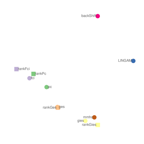
Figure 1: A multi-dimensional scaling visualization of the methods considered. The distance between two methods is taken to be the Euclidean distance between the equal-error-rate of both methods across all settings for the isAncestor query. The MDS plot uses least-squares scaling.

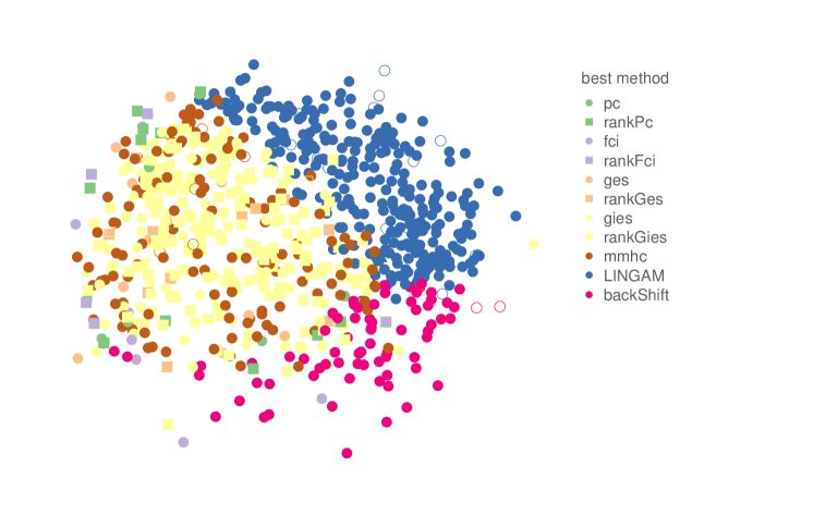
Figure 2: A multi-dimensional scaling visualization of the simulation settings. The distance between two simulation settings is taken to be the correlation distance between the equal-error-rate of both simulation settings across all methods for the isAncestor query. Each setting is shown as a sample point with color coding for the best performing method. A filled symbol indicates that the performance metric was smaller than 0.3 and an un-filled symbol that it was above. MDS uses least-squares scaling.

4.3.1 Multi-dimensional scaling

For each simulation setting and each method, we compute the equal-error-rate for the isAncestor query. This yields a (nr of simulation settings) $\times$ (nr of methods) matrix with E-ER values. The Euclidean distance between two columns in this matrix is a distance between methods. Similarly, the Euclidean distance between two rows in the matrix is a distance between simulation settings.

Figure 1 shows an MDS plot based on distances between the methods, using least-squares scaling. We see that the rank-based methods rankFCI, rankPC, rankGES and rankGIES are close to their counterparts FCI, PC, GES and GIES. It is somewhat unexpected that MMHC is closer to GIES and rankGIES than to PC and GES. The two methods that have the largest average distance to the other methods are LINGAM and BACKSHIFT. This is perhaps expected as these methods are of a very different nature than the other methods.

Figure 2 shows an MDS plot based on distances between the simulation settings, again using least-squares scaling. Thus, each point in the plot now corresponds to a simulation setting. The points are colored according to the best performing method. We see that the regions where either LINGAM or BACKSHIFT are optimal are relatively well separated, while the regions where GIES, MMHC, PC, GES, FCI or their rank-based versions are optimal, do not show a clear separation, as perhaps already expected from the previous result in Figure 1.

4.3.2 Pairwise comparisons

Table 2: A pairwise comparison. Each column shows the percentage of settings where methods were better by a margin of at least 0.1 in the equal-error-rate compared to method in the given column. For example, LINGAM beats PC in $14\%$ of the settings, while PC beats LINGAM by the given marge in $29\%$ of the settings. There is no globally dominant algorithm and a block-structure among related algorithms is visible.

	PC	rankPC	FCI	rankFCI	GES	rankGES	GIES	rankGIES	MMHC	LINGAM	BACKSHIFT
PC	$0$	$6$	$10$	$16$	$1$	$1$	$1$	$0$	$0$	$14$	$20$
rankPC	$0$	$0$	$9$	$10$	$1$	$2$	$0$	$0$	$0$	$11$	$17$
FCI	$1$	$9$	$0$	$5$	$1$	$1$	$1$	$0$	$0$	$11$	$17$
rankFCI	$0$	$1$	$0$	$0$	$1$	$1$	$0$	$0$	$0$	$10$	$16$
GES	$5$	$15$	$16$	$23$	$0$	$0$	$1$	$0$	$0$	$16$	$26$
rankGES	$6$	$15$	$16$	$24$	$0$	$0$	$1$	$0$	$1$	$16$	$25$
GIES	$18$	$29$	$26$	$35$	$10$	$11$	$0$	$0$	$2$	$25$	$35$
rankGIES	$26$	$36$	$34$	$44$	$17$	$17$	$4$	$0$	$1$	$27$	$38$
MMHC	$21$	$33$	$30$	$40$	$16$	$17$	$5$	$0$	$0$	$23$	$36$
LINGAM	$29$	$34$	$34$	$38$	$27$	$27$	$19$	$14$	$14$	$0$	$31$
BACKSHIFT	$18$	$23$	$24$	$29$	$16$	$16$	$9$	$5$	$7$	$13$	$0$

Next, we investigate whether there are methods that dominate the others. We compare the equal-error-rate across all different settings in Table 2. It is apparent that no such dominance is visible among different pairs of methods. A block-structure is visible, however, with similar groups as in Figure 1. One block is formed by the constraint-based methods {PC, rankPC, FCI, rankFCI}: the equal-error-rate of constraint-based methods is hardly ever substantially different. The second block is formed by the score-based approaches {GES, rankGIES} and the third given by the extensions and hybrid methods {GIES, rankGIES, MMHC}. This latter block is of interest as MMHC makes fewer assumptions about the available data and does not need to know where interventions occurred. LINGAM and BACKSHIFT, on the other hand, do not fit nicely into any block in the empirical comparison and are more orthogonal to the other algorithms in that they perform substantially better and substantially worse in many settings, if compared to the other approaches.

Table 3: Marginal rank correlations between equal-error-rate performance (for the isAncestor query) on the one hand and parameters settings on the other hand (shown only if absolute value exceeds 0.1, multiplied by 100 and rounded to the nearest multiple of 5). A positive value for $p$ indicates, for example, that the method becomes less successful with increasing $p$.

	PC	rankPC	FCI	rankFCI	GES	rankGES	GIES	rankGIES	MMHC	LINGAM	BACKSHIFT
n		$15$		$10$							-$15$
p	$45$	$45$	$25$	$25$	$40$	$35$	$35$	$40$	$45$	$40$	$75$
$\mathrm{df}_{\varepsilon}$										$15$
$\rho_{\varepsilon}$	$50$	$60$	$55$	$60$	$55$	$55$	$65$	$50$	$50$	$35$
$\omega$	$10$	$10$	$10$	$10$	$15$	$10$	$20$	$15$	$10$		$20$
$p_{s}$	$20$	$15$	$20$	$15$	$25$	$25$	$25$	$30$	$30$	$15$	$25$
do-interv			-$10$	-$10$
$n_{I}$
$\sigma_{Z}$	-$35$	-$25$	-$35$	-$30$	-$35$	-$35$	-$25$	-$35$	-$30$		-$30$
cyclic			-$15$	-$15$						$35$
$w_{c}$			-$15$	-$15$						$35$
nonlinear										$20$

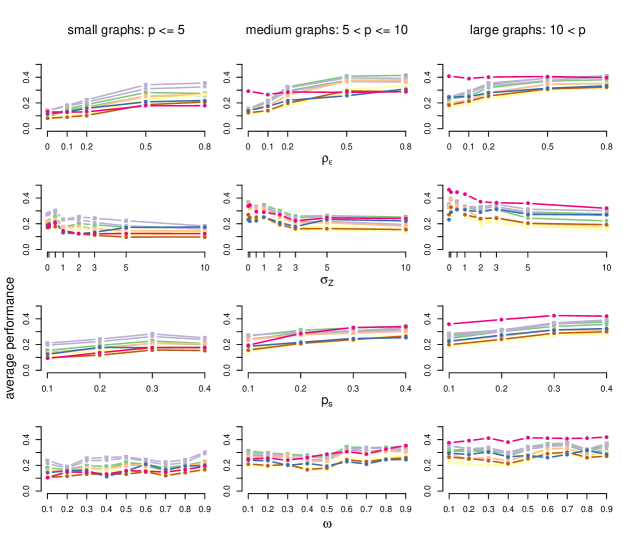
Figure 3: The average equal-error-rate for the isAncestor query, for each method as a function for the four most important parameters (besides the number of variables $p$). The left column shows results for small graphs ($p\leq 5$), the middle column intermediate graphs ($5<p\leq 10$), and the right column for large graphs ($p>10$). The color coding is identical to previous plots.

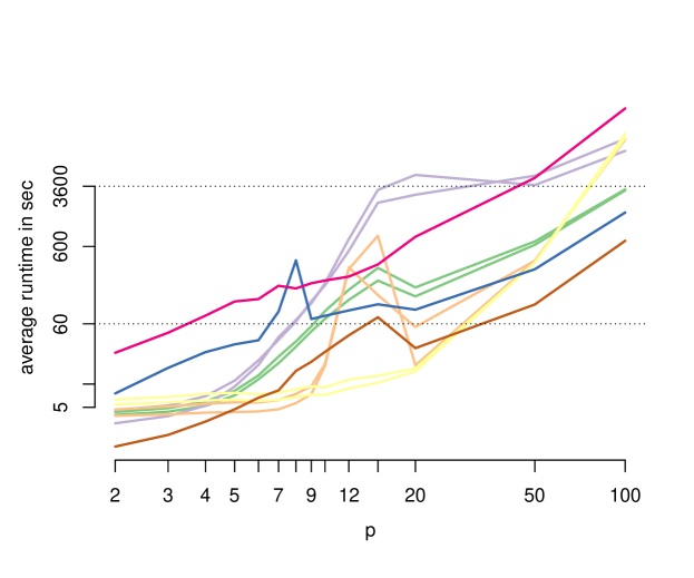
Figure 4: The average runtime in seconds of each method on a logarithmic scale as a function of the number of variables $p$ on a logarithmic scale. A minute and one hour is shown as horizontal bars. The time includes the stability ranking. A single run is faster by a factor of 100 for all methods. (A single run of BACKSHIFT already includes ten subsamples.)

4.3.3 Which causal graphs can be estimated well?

Which graphs can be estimated by some or all methods? To start answering the question, we show in Table 3 the rank correlation between the equal-error-rate for the isAncestor query and parameter settings for all methods. We see that the number of variables $p$ and the strength of the hidden variables $\rho_{\varepsilon}$ show the highest correlations. In both cases the correlation is positive, indicating that increased $p$ or $\rho_{\varepsilon}$ leads to higher equal-error-rates. Other parameters that show substantial correlations are $\omega$, $p_{s}$ and $\sigma_{Z}$. For $\omega$ and $p_{s}$ we again see positive correlations, indicating that large noise contributions and denser graphs are associated with higher equal-error-rates. The correlation with $\sigma_{Z}$ is negative for all methods except for LINGAM. While it is expected that BACKSHIFT benefits from strong interventions, the benefit for for example PC and FCI is unexpected.

We note that the strong effect of $\rho_{\varepsilon}$ can be explained by the fact that we created a correlation $\rho_{\varepsilon}$ between all pairs of noise variables. It is not surprising that this has a larger impact than adding for example a single cycle to the graph (which only seems to substantially affect the performance of LINGAM).

Figure 4 shows the average equal-error-rate for the isAncestor query for each method as a function of the simulation parameters $\rho_{\varepsilon}$, $\omega$, $p_{s}$ and $\sigma_{Z}$ as identified from Table 3, split according to the number of variables $p$ in the graph (small, medium-sized and large graphs). Again, we see that the size of the graph $p$ and the strength of the hidden variables $\rho_{\varepsilon}$ have the strongest effect on performance, with the exception that BACKSHIFT is not much affected by $\rho_{\varepsilon}$ (but which is also perhaps less competitive in the absence of latent confounding). The strength of the interventions, the sparsity of the graph and the signal-to-noise ratio also affect the average performance but perhaps to a lesser extent.

Some other observations:

1. The most surprising outcome is perhaps that the number of samples $n$ has only a very weak influence on the success despite it being varied between a few hundred and twenty thousand.

2. Sparser graphs with fewer edges are consistently easier to estimate with all methods than dense graphs.

3. Less heavy tails in the error distribution have an adverse effect on the performance of LINGAM only, as it makes use of higher moments. LINGAM is also most affected when each variable undergoes a nonlinear transformation.

4. A cycle in the graph again has a detrimental effect on LINGAM (which is likely different in the version of LINGAM that allows for cycles (Lacerda et al., 2008)).

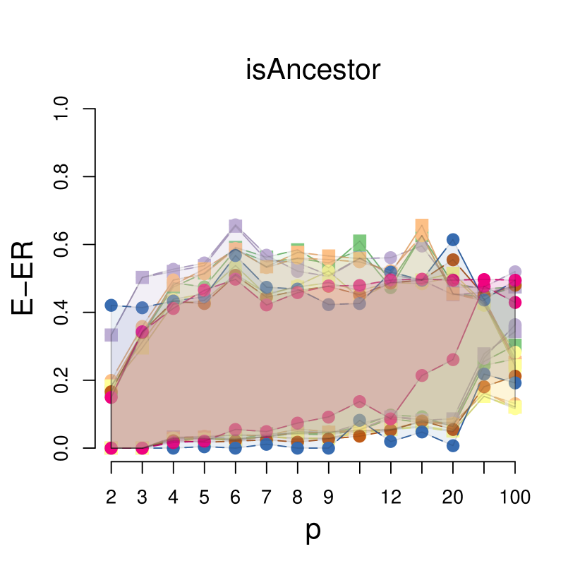
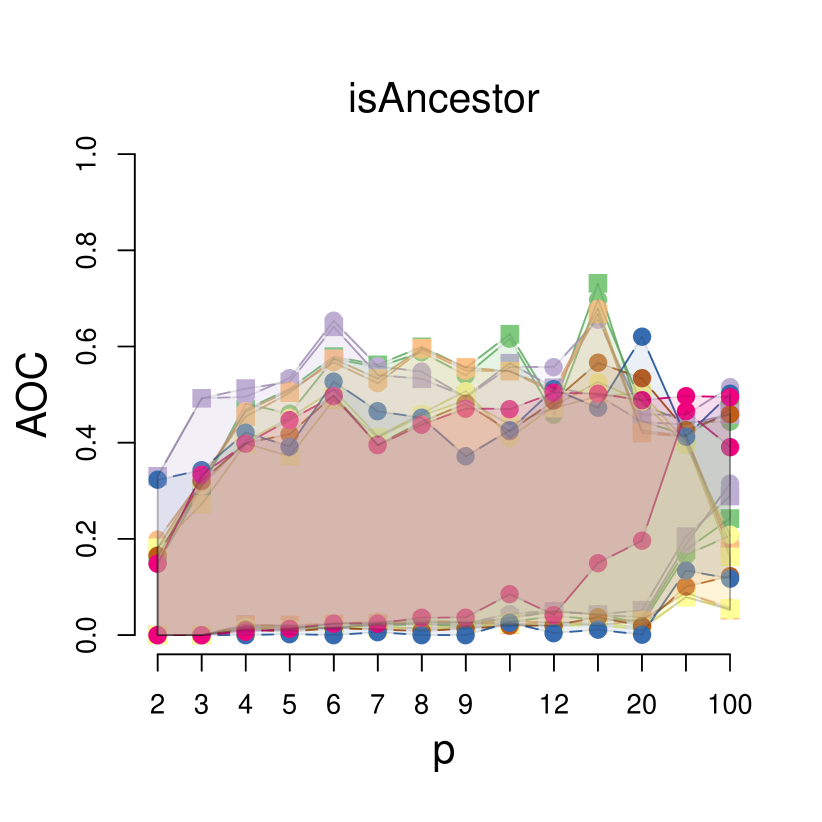
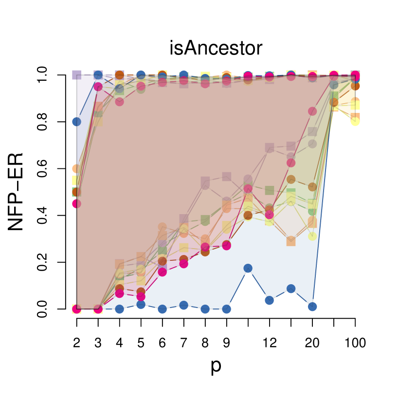
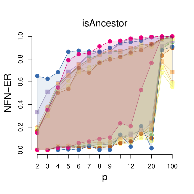
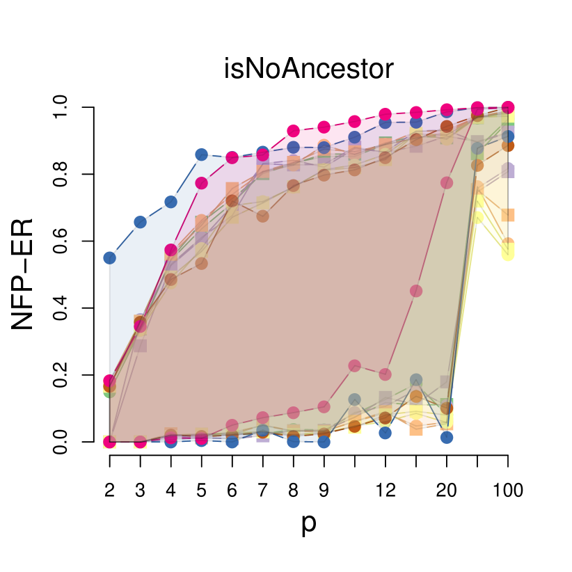
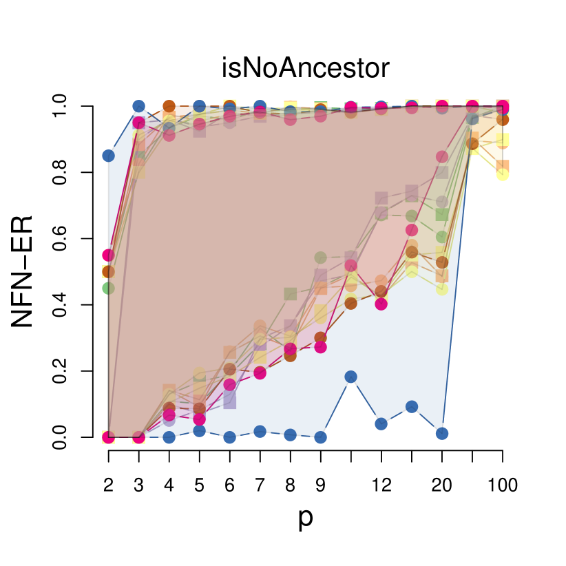
Figure 5: The range of equal-error rate (E-ER) for all methods as a function of the number of variables $p$ for the isAncestor query (top left). Top right shows the same for the area-above-curve (AOC), while second row shows the no-false-positives-error-rate (NFP-ER) and no-false-negatives-error-rate (NFN-ER). The last row contains the corresponding plots to the second row but for the isNoAncestor query.

4.3.4 Bounds on performance

The outcome of the simulations show a large degree of variation. To further investigate the role of the number of variables $p$, we show in Figure 5 the bounds of the performance as a function of $p$ for the isAncestor query. Specifically, for each value of $p$, we consider the range of the four considered metrics when varying all other parameters for each method and show the lower and upper bounds in the figure.

The upper bounds show the worst performance across all parameters while holding $p$ constant. It can be compared to the expected value under random guessing which is 0.5 for the E-ER and AOC metrics and 1 for NFP-ER and NFN-ER.

The lower bound reveals in contrast the error rates in the best setting for a given $p$. The metric NFP-ER seems more difficult to keep at reasonable levels than NFN-ER, with the exception of LINGAM which has very small values of NFP-ER in some settings up to $p\approx 20$. The NFN-ER rate is typically lower than NFP-ER as there are typically more non-ancestral pairs in the graphs (due to not connected components for example) as ancestral pairs. This is confirmed by the third row of panels in Figure 5 which shows the error rates for the isNoAncestor query. Here the roles of NFN-ER and NFP-ER are reversed due to the relative abundance of non-ancestral pairs.

5 DISCUSSION

We have tried to give a contemporaneous overview of structure learning for causal models that are available in R and conducted an extensive empirical comparison. It is noteworthy that we found a clustering of methods into constraint-based, score-based, and other approaches that do not fall neatly into these categories. Methods from the same class behave empirically very similar. We also tried to quantify to what extent methods are negatively or positively affected by various parameters such as the size of the graph to learn, sparsity and strength of hidden variables. The most important parameters in our set-up are the size of the graph $p$ and the strength of the hidden variables $\rho_{\varepsilon}$. An easily accessible interface to all methods is contributed as R-package CompareCausalNetworks.

The results suggest that more efficient algorithms would be desirable, both from a computational and from a statistical point-of-view. As it stands, the success of the algorithms depends on both the assumptions made about the data generating process (and how accurate these assumptions are) and the specific implementation details of each algorithm. It would be worthwhile if the relative importance of these two factors could be separated better by more modular estimation methods and perhaps more work on worst-case bounds. These latter bounds would allow to quantify to what extent the empirically poor statistical scalability is inherent to the problem or a consequence of choices made in the considered algorithms.

6 APPENDIX

6.1 Considered tuning parameter configurations

All methods were run through the interface offered by the CompareCausalNetworks package (Heinze-Deml and Meinshausen, 2017). Below we also indicate the R packages from which the CompareCausalNetworks package calls the respective methods.

backShift

Code available from the R package backShift (Heinze-Deml, 2017).

• covariance $\in\{\texttt{TRUE, FALSE}\}$

• ev $\in\{0.1,0.25,0.5\}\cdot p$

• threshold $=0.75$

• nsim $=10$

• sampleSettings $=1/sqrt(2)$

• sampleObservations $=1/sqrt(2)$

• nodewise = TRUE

• tolerance $=10^{-4}$

GES and rankGES

Code available from the R packages pcalg (Kalisch et al., 2012) (GES) and CompareCausalNetworks (rankGES).

• phase = ’turning’

• score = GaussL0penObsScore

• $\lambda\in\{0.05\log{n},0.5\log{n},5\log{n}\}$

• adaptive = "none"

• maxDegree = integer(0)

GIES and rankGIES

Code available from the R packages pcalg (Kalisch et al., 2012) (GIES) and CompareCausalNetworks (rankGIES).

• phase = ’turning’

• score = GaussL0penObsScore

• $\lambda\in\{0.05\log{n},0.5\log{n},5\log{n}\}$

• adaptive = "none"

• maxDegree = integer(0)

FCI and rankFCI

Code available from the R packages pcalg (Kalisch et al., 2012) (FCI) and CompareCausalNetworks (rankFCI).

• conservative = FALSE and maj.rule = FALSE

• conservative = TRUE and maj.rule = FALSE

• conservative = FALSE and maj.rule = TRUE

• alpha $\in\{0.001,0.01,0.1\}$

• indepTest = gaussCItest

• skel.method = "stable"

• m.max = Inf

• pdsep.max = Inf

• rules = rep(TRUE,10)

• NAdelete = TRUE

• doPdsep = TRUE

• biCC = FALSE

MMHC

Code available from the R package bnlearn (Scutari, 2010).

• $\lambda\in\{0.05\log{n},0.5\log{n},5\log{n}\}$

• alpha $\in\{0.001,0.01,0.1\}$

• whitelist = NULL

• blacklist = NULL

• test = NULL – corresponds to correlation

• score = NULL – corresponds to BIC

• B = NULL

• restart = 0

• perturb = 1

• max.iter = Inf

• optimized = TRUE

• strict = FALSE

PC and Rank PC

Code available from the R packages pcalg (Kalisch et al., 2012) (PC) and CompareCausalNetworks (rankPC).

• conservative = FALSE and maj.rule = FALSE

• conservative = TRUE and maj.rule = FALSE

• conservative = FALSE and maj.rule = TRUE

• alpha $\in\{0.001,0.01,0.1\}$

• indepTest = gaussCItest

• NAdelete = TRUE

• m.max = Inf

• u2pd = "relaxed"

• skel.method = "stable"

• solve.confl = FALSE

6.2 Simulation settings

The results in this work are based on 842 unique simulation settings. The tables below show for each parameter in the data generation scheme how many settings were generated for each considered value for the given parameter.

Sample size

$n$	500	2000	5000	10000
# of settings	231	200	217	194

Number of variables

$p$	2	3	4	5	6	7	8	9	10	12	15	20	50	100
# of settings	71	89	84	77	62	60	74	68	62	76	60	43	8	8

Edge density parameter

$p_{s}$	0.1	0.2	0.3	0.4
# of settings	202	226	200	214

Number of settings

$n_{I}$	3	4	5
# of settings	271	275	296

Intervention type

	shift intervention	do-intervention
# of settings	417	425

Strength of the interventions

$\sigma_{Z}$	0	0.1	0.5	1	2	3	5	10
# of settings	111	105	102	105	106	98	116	99

Degrees of freedom of the noise distribution

$df_{\varepsilon}$	2	3	5	10	20	100
# of settings	140	136	147	140	144	135

Strength of hidden variables

$\rho_{\varepsilon}$	0	0.1	0.2	0.5	0.8
# of settings	161	164	166	179	172

Proportion of variance from noise

$\omega$	0.1	0.2	0.3	0.4	0.5	0.6	0.7	0.8	0.9
# of settings	116	85	88	110	85	91	82	91	94

Settings with cycles

no cycles cycles # of settings 576 266

Strength of cycle

$w_{c}$	0	0.1	0.25	0.5	0.75	0.9
# of settings	576	56	51	50	55	54

Settings with model misspecification

	no model misspecification	model misspecification
# of settings	715	127

References

- Ali et al. (2009) R. Ayesha Ali, Thomas S. Richardson, and P. Spirtes. Markov equivalence for ancestral graphs. Ann. Stat., 37:2808–2837, 2009.
- Andersson et al. (1997) S.A. Andersson, D. Madigan, and M.D. Perlman. A characterization of Markov equivalence classes for acyclic digraphs. Annals of Statistics, 25:505–541, 1997.
- Angrist et al. (1996) J. D. Angrist, G. W. Imbens, and D. B. Rubin. Identification of causal effects using instrumental variables. Journal of the American Statistical Association, 91:444–455, 1996.
- Chickering (2002a) D. M. Chickering. Learning equivalence classes of Bayesian-network structures. Journal of Machine Learning Research, 2:445–498, 2002a.
- Chickering (2002b) D. M. Chickering. Optimal structure identification with greedy search. Journal of Machine Learning Research, 3:507–554, 2002b.
- Cho et al. (2014) S. W. Cho, S. Kim, Y. Kim, J. Kweon, H. S. Kim, S. Bae, and J.-S. Kim. Analysis of off-target effects of CRISPR/Cas-derived RNA-guided endonucleases and nickases. Genome Research, 24:132–141, 2014.
- Claassen et al. (2013) T. Claassen, J. M. Mooij, and T. Heskes. Learning sparse causal models is not NP-hard. In Proceedings of the 29th Annual Conference on Uncertainty in Artificial Intelligence (UAI), 2013.
- Colombo and Maathuis (2014) D. Colombo and M. H. Maathuis. Order-independent constraint-based causal structure learning. J. Mach. Learn. Res., 15:3741–3782, 2014.
- Colombo et al. (2012) D. Colombo, M. H. Maathuis, M. Kalisch, and T. S. Richardson. Learning high-dimensional directed acyclic graphs with latent and selection variables. Annals of Statistics, 40:294–321, 2012.
- Comon (1994) P. Comon. Independent component analysis, a new concept? Signal processing, 36:287–314, 1994.
- Cooper and Yoo (1999) G. Cooper and C. Yoo. Causal discovery from a mixture of experimental and observational data. In Proceedings of the 15th Annual Conference on Uncertainty in Artificial Intelligence (UAI), pages 116–125, 1999.
- Dawid (2000) A. P. Dawid. Causal inference without counterfactuals. Journal of the American Statistical Association, 95:407–424, 2000.
- Didelez (2017) V. Didelez. Handbook of Graphical Models, chapter Causal Concepts and Graphical Models. Chapman & Hall/CRC, 2017. To appear.
- Drton and Maathuis (2017) M. Drton and M. H. Maathuis. Structure learning in graphical modeling. Annual Review of Statistics and Its Application, 4:365–393, 2017.
- Eaton and Murphy (2007) D. Eaton and K. P. Murphy. Exact Bayesian structure learning from uncertain interventions. In Proceedings of the 11th International Conference on Artificial Intelligence and Statistics (AISTATS), pages 107–114, 2007.
- Frisch (1938) R. Frisch. Autonomy of economic relations: Statistical versus theoretical relations in economic macrodynamics. Paper given at League of Nations. Reprinted in D.F. Hendry and M.S. Morgan (1995), The Foundations of Econometric Analysis, Cambridge University Press, 1938.
- Haavelmo (1944) T. Haavelmo. The probability approach in econometrics. Econometrica, 12:S1–S115 (supplement), 1944.
- Harris and Drton (2013) N. Harris and M. Drton. PC algorithm for nonparanormal graphical models. Journal of Machine Learning Research, 14:3365–3383, 2013.
- Hauser and Bühlmann (2012) A. Hauser and P. Bühlmann. Characterization and greedy learning of interventional Markov equivalence classes of directed acyclic graphs. Journal of Machine Learning Research, 13:2409–2464, 2012.
- Heinze-Deml (2017) C. Heinze-Deml. backShift: Learning Causal Cyclic Graphs from Unknown Shift Interventions, 2017. URL https://github.com/christinaheinze/backShift. R package version 0.1.4.1.
- Heinze-Deml and Meinshausen (2017) C. Heinze-Deml and N. Meinshausen. CompareCausalNetworks: Interface to Diverse Estimation Methods of Causal Networks, 2017. URL https://github.com/christinaheinze/CompareCausalNetworks. R package version 0.1.6.
- Hoyer et al. (2008) P. O. Hoyer, S. Shimizu, A. J. Kerminen, and M. Palviainen. Estimation of causal effects using linear non-Gaussian causal models with hidden variables. Int. J. Approx. Reasoning, 49:362–378, 2008.
- Hyttinen et al. (2012) A. Hyttinen, F. Eberhardt, and P. O. Hoyer. Learning linear cyclic causal models with latent variables. Journal of Machine Learning Research, 13:3387–3439, 2012.
- Imbens (2014) G. Imbens. Instrumental variables: An econometrician’s perspective. Statistical Science, 29:323–358, 2014.
- Kalisch and Bühlmann (2007) M. Kalisch and P. Bühlmann. Estimating high-dimensional directed acyclic graphs with the PC-algorithm. Journal of Machine Learning Research, 8:613–636, 2007.
- Kalisch et al. (2012) M. Kalisch, M. Mächler, D. Colombo, M. H. Maathuis, and P. Bühlmann. Causal inference using graphical models with the R package pcalg. Journal of Statistical Software, 47(11):1–26, 2012.
- Lacerda et al. (2008) G. Lacerda, P. Spirtes, J. Ramsey, and P.O. Hoyer. Discovering cyclic causal models by independent components analysis. In Proceedings of the 24th Conference on Uncertainty in Artificial Intelligence (UAI), pages 366–374, 2008.
- Lauritzen (1996) S. L. Lauritzen. Graphical Models. Oxford University Press, New York, USA, 1996.
- Maathuis et al. (2009) M. H. Maathuis, M. Kalisch, and P. Bühlmann. Estimating high-dimensional intervention effects from observational data. Annals of Statistics, 37:3133–3164, 2009.
- Maathuis et al. (2010) M. H. Maathuis, D. Colombo, M. Kalisch, and P. Bühlmann. Predicting causal effects in large-scale systems from observational data. Nature Methods, 7:247–248, 2010.
- Nandy et al. (2017a) P. Nandy, A. Hauser, and M. H. Maathuis. High-dimensional consistency in score-based and hybrid structure learning. 2017a. arXiv:1507.02608.
- Nandy et al. (2017b) P. Nandy, M. H. Maathuis, and T. S. Richardson. Estimating the effect of joint interventions from observational data in high-dimensional settings. Annals of Statistics, 45:647–674, 2017b.
- Pearl (2009) J. Pearl. Causality: Models, Reasoning, and Inference. Cambridge University Press, New York, USA, 2nd edition, 2009.
- Peters et al. (2016) J. Peters, P. Bühlmann, and N. Meinshausen. Causal inference using invariant prediction: identification and confidence intervals. Journal of the Royal Statistical Society, Series B, 78:947–1012, 2016.
- R Core Team (2017) R Core Team. R: A Language and Environment for Statistical Computing. R Foundation for Statistical Computing, Vienna, Austria, 2017. URL https://www.R-project.org/.
- Richardson and Robins (2013) T. Richardson and J. M. Robins. Single world intervention graphs (SWIGs): A unification of the counterfactual and graphical approaches to causality. Center for the Statistics and the Social Sciences, University of Washington Series. Working Paper 128, 30 April 2013, 2013.
- Richardson and Spirtes (1999) T. Richardson and P. Spirtes. Automated discovery of linear feedback models. In C. Glymour and G.F. Cooper, editors, Computation, Causation, and Discovery, pages 253–304. MIT Press, 1999.
- Richardson and Spirtes (2002) T. Richardson and P. Spirtes. Ancestral graph Markov models. Annals of Statistics, 30:962–1030, 2002.
- Robins (1986) J. M. Robins. A new approach to causal inference in mortality studies with a sustained exposure period – application to control of the healthy worker survivor effect. Mathematical Modelling, 7:1393 – 1512, 1986.
- Rothenhäusler et al. (2015) D. Rothenhäusler, C. Heinze, J. Peters, and N. Meinshausen. backShift: Learning causal cyclic graphs from unknown shift interventions. In Advances in Neural Information Processing Systems 28 (NIPS), pages 1513–1521, 2015.
- Rubin (2005) D. B. Rubin. Causal inference using potential outcomes. Journal of the American Statistical Association, 100:322–331, 2005.
- Scutari (2010) M. Scutari. Learning bayesian networks with the bnlearn R package. Journal of Statistical Software, 35(3):1–22, 2010. URL http://www.jstatsoft.org/v35/i03/.
- Shimizu et al. (2006) S. Shimizu, P. O. Hoyer, A. Hyvärinen, and A.J. Kerminen. A linear non-Gaussian acyclic model for causal discovery. Journal of Machine Learning Research, 7:2003–2030, 2006.
- Shimizu et al. (2011) S. Shimizu, T. Inazumi, Y. Sogawa, A. Hyvärinen, Y. Kawahara, T. Washio, P. O. Hoyer, and K. Bollen. DirectLiNGAM: A direct method for learning a linear non-Gaussian structural equation model. Journal of Machine Learning Research, 12:1225–1248, 2011.
- Spirtes et al. (1999) P. Spirtes, C. Meek, and T.S. Richardson. Computation, Causation and Discovery, chapter An algorithm for causal inference in the presence of latent variables and selection bias, pages 211–252. MIT Press, 1999.
- Spirtes et al. (2000) P. Spirtes, C. Glymour, and R. Scheines. Causation, Prediction, and Search. MIT Press, Cambridge, USA, 2nd edition, 2000.
- Stekhoven et al. (2012) D.J. Stekhoven, I. Moraes, G. Sveinbjörnsson, L. Hennig, M.H. Maathuis, and P. Bühlmann. Causal stability ranking. submitted, 2012.
- Tian and Pearl (2001) J. Tian and J. Pearl. Causal discovery from changes. In Proceedings of the 17th Conference Annual Conference on Uncertainty in Artificial Intelligence (UAI), pages 512–522, 2001.
- Tsamardinos et al. (2006) I. Tsamardinos, L. E. Brown, and C. F. Aliferis. The max-min hill-climbing Bayesian network structure learning algorithm. Machine Learning, 65:31–78, 2006.
- Wright (1934) D. Wright. The method of path coefficients. Annals of Mathematical Statistics, 5:161–215, 1934.
- Wright (1921) S. Wright. Correlation and causation. Journal of Agricultural Research, 20:557–585, 1921.
- Zhang (2008a) J. Zhang. Causal reasoning with ancestral graphs. Journal of Machine Learning Research, 9:1437–1474, 2008a.
- Zhang (2008b) J. Zhang. On the completeness of orientation rules for causal discovery in the presence of latent confounders and selection bias. Artificial Intelligence, 172:1873–1896, 2008b.