Influence Networks in International Relations

Abstract.

Measuring influence and determining what drives it are persistent questions in political science and in network analysis more generally. Herein we focus on the domain of international relations. Our major substantive question is: How can we determine what characteristics make an actor influential? To address the topic of influence, we build on a multilinear tensor regression framework (MLTR) that captures influence relationships using a tensor generalization of a vector autoregression model. Influence relationships in that approach are captured in a pair of $n\times n$ matrices and provide measurements of how the network actions of one actor may influence the future actions of another. A limitation of the MLTR and earlier latent space approaches is that there are no direct mechanisms through which to explain why a certain actor is more or less influential than others. Our new framework, social influence regression, provides a way to statistically model the influence of one actor on another as a function of characteristics of the actors. Thus we can move beyond just estimating that an actor influences another to understanding why. To highlight the utility of this approach, we apply it to studying monthly-level conflictual events between countries as measured through the Integrated Crisis Early Warning System (ICEWS) event data project.

Motivation

The concepts of power and influence are gold-standard building blocks in analyses of world politics. Well-known debates on these blocks in early works include Von Clausewitz (1832); Haas (1953); Fucks (1965); Keohane and Nye (1977); Baldwin (1978); Rummel (1979); Waltz (1979). In the 1980s and 1990s, scholars also struggled with the meaning of power and influence in world affairs (Doran and Parsons, 1980; Keohane, 1989; Gowa and Mansfield, 1993). This continues to the present as scholars look forward as well as backward into history (Kadera, 2001; Barnett and Duvall, 2004; Nexon, 2009). Despite the nearly ubiquitous use of the concept of power, and its derivative concept influence, there is no agreed upon way to assess this feature of world politics. Indeed not only is there no agreement on how to measure this concept, there is little agreement on exactly what it means conceptually. Is power based on military capabilities? On, diplomatic prowess? The notions of power and influence imply relations among political actors such as countries, and as such they may be best thought of a relational characteristics rather than material ones. Herein we address a way of examining one type of influence within a specific network framework. The ability of one actor in world politics to influence another is intimately tied to other actors in the world. Sometimes it is quite overt as when the US calls for China to influence North Korea. Other times these linkages and dependencies may be more diffuse and spread out, as when a coalition of 31 countries influence Iraq to withdraw its forces from Kuwait. We develop a network approach to show how these kinds of dependencies can be studied.

Relational data defines connections between pairs of actors – also known as dyads. These connections can take the shape of simple undirected, binary relations observed for a snapshot in time to complex types of directed and weighted relations that are observed longitudinally. The study of these types of relations is almost ubiquitous in scholarly work. In genetics, researchers have defined actors as proteins and links as the bonds between them (Wu et al., 2009; Welch, Bansal and Hunter, 2011; Livi et al., 2016). Whereas in the social sciences, researchers have applied network analysis to the study of terrorist networks, legislators in Congress, and the diffusion of civil wars (de Bie et al., 2017; Cho and Fowler, 2010; Metternich, Minhas and Ward, 2015). The study of these types of data is made more interesting by the possibility that the relations observed do not arise or evolve independent of one another. Observations in relational data may be simultaneously dependent on all other observations due to the social ties and pathways that give shape to the global structure in which actors are embedded. This dependence is why many study relational data not as a set of independent dyadic observations, but as a network in which the link between a pair of actors influences and is influenced by other dyads. Characterizing the manner in which observations are interdependent and then using those interdependencies to examine the emergence and evolution of a network is a principal focus of social network analysis.

A popular approach framework through which to characterize interdependencies are latent variable models, such as the latent class (Snijders and Nowicki, 1997), distance (Hoff, Raftery and Handcock, 2002), and factor models (Hoff, 2005). Each of these model broader patterns—such as homophily and stochastic equivalence—as a function of node-specific latent variables. These approaches are effective at characterizing influence patterns that emerge in the network, but they are only able to explain those patterns through endogenous explanations. For example, actors that cluster together in the Euclidean space estimated from latent distance models or that are assigned to similar blocks by latent class models are assumed to possess some set of similar characteristics based on dependence patterns in the network. Yet, these approaches leave unanswered the question of what those characteristics are?

To address this broader question, we build on the bilinear network autoregression model introduced by Hoff (2015) and Minhas, Hoff and Ward (2016). At its core, this approach is a vector autoregression model extended to handle relational data. Within this approach dependencies between observations are captured by a pair of $n\times n$ matrices that measure sender- and receiver-level influence patterns. The model takes the following form: $y_{ij,t}=\sum a_{ii^{\prime}}b_{jj^{\prime}}x_{i^{\prime}j^{\prime},t-1}+e_{ij}$. The term $a_{i,i^{\prime}}$ captures how previous actions of $i^{\prime}$ affect those of $i$ and $b_{j,j^{\prime}}$ shows how actions towards target $j$ are influenced by prior actions toward $j^{\prime}$. To characterize influence patterns via a set of exogenous attributes we rewrite the influence parameters so that they depend on covariates. This enables us to reduce the bilinear model into a rank one regression model: $y_{ij,t}=\alpha^{\prime}X_{ij,t-1}\beta+e_{ij}$ that we refer to as the social influence regression (SIR) model.

The simplification of the bilinear autoregression model allows us to incorporate actor and dyad-level covariate information into determining influence patterns within the network. We apply this approach to data from the Integrated Crisis Early Warning System (ICEWS) event data project. The ICEWS event data are constructed by applying natural language processing and graph theory techniques (Boschee, Natarjan and Weischedel, 2013) to a corpus of about 30 million media reports from about 275 local and global news sources in or translated to English. Each media report is coded in accordance with an ontology of events that is derived from the Conflict and Median Event Observation (CAMEO) scheme (Schrodt, Gerner and Yilmaz, 2009). Our focus for this project is centered around modeling monthly level material conflict events as tracked by ICEWS. With the SIR model we can estimate the extent to which actors within the material conflict network influence one another, and, for example, explore whether or not characteristics such as a pair of countries being allied is related to the influence of one on another. Finally, we show that this network-based approach to understanding the evolution of the material conflict network has substantially better out-of-sample performance than extant approaches employed in the literature.

Methods

Bilinear network autoregression model

Many studies examine the flows or linkages among actors, such as whether two countries are in a conflict with one another. Data from such studies can be thought of relational data which is often represented in the form of a matrix as shown in Figure 2. This matrix $n\times n$ where $n$ denotes the number of actors in the network. The off-diagonals of represent the interaction that took place between two actors, so $y_{ij}$ represents an interaction that took place between actors $i$ and $j$. In the case of undirected data, this may simply be an indicator that $i$ and $j$ are allied to one another. For directed data, the rows designate the senders of a particular action and the columns the receiver, so the $y_{ij}$ entry would represent an action sent from $i\rightarrow j$. The diagonals are typically undefined indicating that actors do not interact with themselves.

$$Y_{t}=\bordermatrix{\leavevmode\nobreak\ &i&\ldots&j&\ldots&k\cr i&NA&\ldots&y_{ji}&\ldots&y_{ik}\cr\vdots&\vdots&\ddots&\vdots&\ddots&\vdots\cr j&y_{ji}&\ldots&NA&\ldots&y_{jk}\cr\vdots&\vdots&\ddots&\vdots&\ddots&\vdots\cr k&y_{ki}&\ldots&y_{kj}&\ldots&NA\cr}$$

Figure 1. Matrix representation of a dyadic, relational measure for one time point.

Figure 2. Array representation of a longitudinal dyadic measure. Darker shading indicates later time periods.

Figure 2 represents the interactions that take place between actors for a snapshot in time. In many fields, such as international relations, a single cross-section of data is insufficient, and we observe a time series of interactions between countries. Extending network approaches to studying longitudinal networks has become a topic of recent attention (Snijders, 2014; Krivitsky and Handcock, 2014; Sewell and Chen, 2015; Schein et al., 2015). To represent longitudinal network structures, we begin by binding adjacency matrices into an array (see Figure 2). Specifically, let $Y=\{Y_{t}:t=1,\ldots,T\}$ be a time series of sociomatrices of relational data where $T$ represents the number of time points, and the dimensions of this object are $n\times n\times T$. Estimating models on structures such as these is the focus of the bilinear autoregression model. The basis of this approach is a first-order vector autoregression model in which we regress the network at one point in time on its lag. The parameters that captures the relationship between them are a pair of matrices that capture sender and receiver dependence patterns for each pair.

More concretely, a generalized bilinear autoregression model for $Y$ is given:

$$E[y_{i,j,t}] =g(\mu_{i,j,t})$$

$$\{\mu_{i,j,t}\} =M_{t}=AX_{t}B^{\top}$$

$$\{\mu_{i,j,t}\} =a_{i}^{\top}X_{t}b_{j}$$

where $x_{i,j,t}$ is a function of $y_{i,j,t}$, such as $\tilde{x}_{i,j,t}\sim\log(y_{i,j,t-1}+1)$.

In the next section we explore an example with count data. Therein $Y$ is a time series of matrices of counts of events between actors. Accordingly, we model $y_{i,j,t}\sim$ Poisson$(e^{\mu_{i,j,t}})$, where $\tilde{x}_{i,j,t}=\log(y_{i,j,t-1}+1)$. The basis of this framework is still a generalized bilinear model so this approach is readily extendable to other distribution types. $A$ and $B$ are $n\times n$ “influence parameters.” The value of $a_{ii^{\prime}}$ captures how predictive the actions of country $i^{\prime}$ at time $t-1$ are of the actions of country $i$ at time $t$, while the value of $b_{jj^{\prime}}$ captures how predictive the actions directed at country $j^{\prime}$ at time $t-1$ are of the actions directed towards country $j$ at time $t$. For example, consider a bilinear autoregression model on conflict that includes the United Kingdom (GBR) and the United States of America (USA). If we estimate that $a_{\text{GBR},\text{USA}}$ is greater than zero, this implies that countries the USA initiated/continued a conflict with in period $t-1$ are likely to also face a conflict from GBR in period $t$. Thus, GBR’s future actions are influenced by the USA, or, put more concretely, actions of the USA are predictive of GBR’s.

Social influence regression

The SIR model explains the influence in terms of covariates and allows us to determine what makes an actor influential. Particularly, to determine the characteristics of $i$ or $i^{\prime}$ that are related to the influence $a_{ii^{\prime}}$, we consider a linear regression model for $a_{ii^{\prime}}$ and $b_{jj^{\prime}}$, given by $a_{ii^{\prime}}=\alpha^{\top}w_{ii^{\prime}}$ and $b_{jj^{\prime}}=\beta^{\top}w_{jj^{\prime}}$, where $w_{ii^{\prime}}$ is a vector of nodal and dyadic covariates specific to pair $ii^{\prime}$ that we are using to estimate influence. The application we present in the following section has time-varying covariates, which this model is able to account for through time varying influence parameters: $a_{ii^{\prime}t}=\alpha^{\top}w_{ii^{\prime}t}$ and $b_{jj^{\prime}t}=\beta^{\top}w_{jj^{\prime}t}$.

The network autoregression model can be expressed as:

$$\mu_{i,j,t} =\sum_{i^{\prime}j^{\prime}}a_{ii^{\prime}t}x_{i^{\prime}j^{\prime}t}b_{jj^{\prime}t}=\sum_{i^{\prime}j^{\prime}}\alpha^{\top}w_{ii^{\prime}t}x_{i^{\prime}j^{\prime}t}w_{jj^{\prime}t}^{\top}\beta$$

$$=\alpha^{\top}\left(\sum_{i^{\prime}j^{\prime}}x_{i^{\prime}j^{\prime}t}w_{ii^{\prime}t}w_{jj^{\prime}t}^{\top}\right)\beta=\alpha^{\top}\tilde{X}_{ijt}\beta$$

Typically, $y_{i,j,t}$ also has covariates. For example, we might want to condition estimation of the parameters on a lagged version of the dependent variable, $y_{i,j,t-1}$, a measure of reciprocity, $y_{j,i,t-1}$, and other exogenous variables. In the case of estimating a model on material conflict between a pair of countries, this might include other exogenous aspects such as the geographical distance between a pair of countries. These additional exogeneous parameters can be accommodated with a model of the form:

$$\mu_{i,j,t}=\theta^{\top}z_{i,j,t}+\alpha^{\top}\tilde{X}_{ijt}\beta,$$

where $z_{i,j,t}$ represents the design array incorporating parameters that may have a direct effect on the dependent variable. The model presented here is a type of low-rank matrix regression: it regresses the outcome $y_{ij,t}$ on the matrix $X_{ij,t}$. An unconstrained (linear) regression would be expressed as $\mu_{ij,t}=\theta^{\top}z_{ij,t}+\langle C,{X}_{ij,t}\rangle$, where $C$ is an arbitrary $p\times p$ matrix of regression coefficients to be estimated. In contrast, the regression specified above restricts $C$ to be rank one, that is, expressible as $C=\alpha\beta^{\top}$. This follows from the identity that $\langle\alpha\beta^{\top},{X}_{ij,t}\rangle=\alpha^{\top}{X}_{ij,t}\beta$. Low rank matrix regression models have been considered by Li, Kim and Altman (2010) and Zhou, Li and Zhu (2013).

Estimation

To estimate the parameters, $\{\theta,\alpha,\beta\}$ we employ an iterative process because the model is bilinear. Specifically, for a fixed $\beta$ the model is linear in $(\theta,\alpha)$. For fixed $\alpha$ the model is linear in $(\theta,\beta)$. Hence:

$$\mu_{i,j,t} =(\theta^{\top}\ \alpha^{\top})\left(\begin{array}[]{c}z_{i,j,t}\\ \tilde{X}_{ijt}\beta\end{array}\right)$$

$$=(\theta^{\top}\ \beta^{\top})\left(\begin{array}[]{c}z_{i,j,t}\\ \tilde{X}_{ijt}^{\top}\alpha\end{array}\right)$$

Maximum likelihood estimate can be obtained with an iterative block coordinate descent method for estimation of $\theta$, $\alpha$ and $\beta$. Given initial values of $\beta$, iterate the following until convergence:

1. Find the conditional maximum likelihood estimate (MLE) of $(\theta,\alpha)$ given $\beta$ using iterative weighted least squares (IWLS);

2. Find the conditional MLE of $(\theta,\beta)$ given $\alpha$ using IWLS.

Using this approach the problem of finding the conditional MLEs turns into a sequence of low dimensional generalized linear model (GLM) optimizations. For example, let $n$ be the number of nodes, $p$ be the length of each $w_{ii^{\prime}}$ vector, and $q$ be the length of each $z_{ij,t}$ vector. Then step one from above can be implemented as follows:

1. Let $\tilde{x}_{ij,t}$ be the vector of length $p+q$ obtained by concatenating $z_{ij,t}$ and $X_{ij,t}\beta$.

2. Construct the matrix $\tilde{X}$ having $n\times(n-1)\times T$ rows and $p+q$ columns, where each row is equal to $\tilde{x}_{ij,t}$ for some (directed) pair $i,j$ at time $t$.

3. Let $y$ be the vector of length $n\times(n-1)\times T$ consisting of the entries of $Y=\{Y_{1},\ldots,Y_{T}\}$, ordered to correspond to the rows of $\tilde{X}$.

4. Obtain the MLEs for the Poisson regression of $y$ on $\tilde{X}$. From the regression coefficients, extract the (conditional) estimates of $\theta$ and $\alpha$.

Step 2 of the iterative algorithm works similarly, by replacing $X_{ij,t}\beta$ in item (a) with $X_{ij,t}^{\top}\alpha$.

Inference

Approximate standard errors and confidence intervals for the parameters can be obtained from the derivatives of the log-likelihood function at the MLE. This claim, however, comes with a caveat: The multiplicative parameters $\alpha$ and $\beta$ are not identifiable, as the term $\alpha^{\top}X\beta$ is the same as $(\alpha/c)^{\top}X(c\beta)$ for any scalar $c$. Meaningful derivative-based standard errors need to be derived from an identifiable parameterization of the model. An identifiable parameterization may be obtained by placing a scale restriction on $\alpha$ or $\beta$, or fixing one element of either. The identifiable parameterization employed herein restricts the first element of $\alpha$ to be one.

Log-likelihood derivatives of the identifiable parameters may be obtained by calculating the derivatives for the unconstrained, non-identifiable parameterization, and then using the chain rule to obtain the derivatives for the constrained, identifiable case. Let $H$ be the matrix of second derivatives of the log-likelihood at the MLE $\hat{\psi}$ of $\psi=(\theta,\alpha,\beta)$ (using an identifiable parameterization). An estimate of the variance of $\hat{\psi}$ is given by $H^{-1}$, and standard errors for $\hat{\psi}$ are given by the square roots of the diagonal elements fof $H^{-1}$. The asymptotic validity of these standard errors relies upon the assumption that the underlying model is correct. Alternatively, model-robust standard errors can be obtained using a Sandwich variance estimate,

$$\widehat{\text{Var}(\hat{\psi})}=H^{-1}SH^{-1}$$

where the matrix $S$ is given by

$$\sum_{i,j,t}(y_{i,j,t}-\mu_{i,j,t})\dot{L}_{ij,t}\dot{L}_{ij,t}^{\top},$$

with $\dot{L}_{ij,t}$ denoting the derivative of the log-likelihood corresponding to the single observation $y_{ij,t}$. In the application that follows we utilize model-robust standard errors.

Figure 3 provides a visual summary of this model. The array in the far left represents the network being modeled, the design array in green represents explanatory variables used to directly model linkages between dyads, and the $\theta$ vector includes the estimates of the effect those variables have on the network. To capture dependence patterns, a logged and lagged version of dependent variable are included, along with a design array containing a set of influence covariates, $W$; $\alpha$ and $\beta$ are vectors that capture parameter estimates for the effects of those influence covariates. A benefit of this framework is that once estimated, linear combinations of the influence regression parameters permit visualization the resulting sender and receiver dependence patterns in the network.

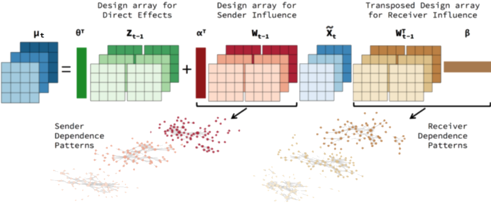
Figure 3. Visual summary of social influence regression model.

Empirical Application

ICEWS Material Conflict

Over the past few years, a number of projects have arisen seeking to create large data sets of dyadic events through the automatic extraction of information from on-line news archives. This has made it empirically easier to study interactions among countries, as well as among actors such as NGOs within countries.

The two most well-known developments include the ICEWS event data project (Boschee et al., 2015a) and the Phoenix pipeline (OEDA, 2016). At present, the field of event data is evolving, but ICEWS remains the gold standard. For the purposes of this project we focus on utilizing the ICEWS database which also extends back farther in time. ICEWS draws from over 300 different international and national focused publishers (Boschee et al., 2015b). The ICEWS event data are based on a continuous monitoring of over 250 news sources and other open source material covering 177 countries worldwide. ICEWS consists of several components, including a database of over 38 million multilingual news stories going back to 1990 and present to last week. The ICEWS data along with extensive documentation have been made publicly available (with a one year embargo) on dataverse.org (Lautenschlager, Shellman and Ward, 2015; Boschee et al., 2015a). To classify news stories into socio-political topics, ICEWS relies on a augmented and expanded version of the CAMEO coding scheme (Schrodt, Gerner and Yilmaz, 2009). The dictionaries, aggregations, ground truth data, and actor and verb dictionaries are publicly available with a one year lag at the ICEWS data repository https://dataverse.harvard.edu/dataverse/icews. In addition, the event coder has been made available publicly by the Office of the Director of National Intelligence. This event coder, known as ACCENT, searches for the following information: a sender, a receiver, an action type, and a time stamp. The set of action types covered include activities between dyads such as “Occupy territory”, “Use conventional force”, and “Impose embargo, boycott, or sanctions”. Then, the ontology provides rules through which the parsed story is coded. An example of a coded news story fitting this last category is:

“President Bill Clinton has imposed sanctions on the Taliban religious faction that controls Afghanistan for its support of suspected terrorist Osama bin Laden, the White House said Tuesday.”

In this example, the actor designated as sending the action is the United States and the actor receiving it is Afghanistan. Dyadic measurements such as these are available for 249 countries, and the dataset is updated regularly. Currently, data up until March 2016 has been made publicly available on the ICEWS dataverse.

Our sample for this analysis focuses on monthly level interactions between countries in the international system from 2005 to 2012. To measure conflict from this database we focus on what is often referred to as the “material conflict” variable. This variable is taken from the “quad variable” framework developed by Duval and Thompson (1980). Schrodt and Yonamine (2013) defines the type of events that get drawn into this category as those involving, “Physical acts of a conflictual nature, including armed attacks, destruction of property, assassination, etc.”.

January 2005
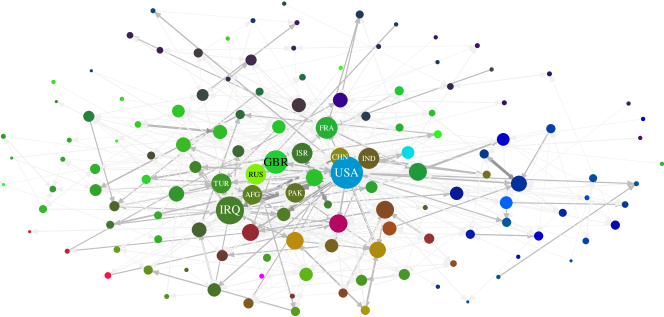
December 2012

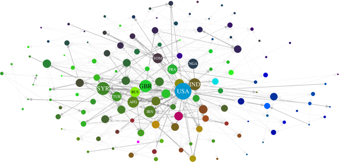
Figure 4. Network depiction of ICEWS Material Conflict events for January 2005 (top) and December 2012 (bottom).

Figure 4 visualizes the material conflict variable as a network, specifically, we provide snapshots of events between dyads along this relational dimension in January 2005 and December 2012. The size of the nodes correspond to how active countries are in the network, and each node is colored by its geographic position. An edge between two nodes designates that at least one material conflict event has taken place between that dyad, and arrows indicate the sender and receiver. Thicker edges indicate a greater count of material conflict events between a dyad.

In both snapshots, the United States is highly involved in conflict events occurring in the system both in 2005 and 2012. Additionally, other major powers such as Russia and the Great Britain are also frequently involved. Some notable changes are visible in the network. While in 2005 Iraq was highly involved in material conflict events by 2012 Syria became more active. Last, there is a significant amount of clustering by geography in this network. Conflict involving Latin American countries is relatively infrequent but when it does occur, it seems to primarily involve countries within the region.

Parameters with direct effect

What variables have a direct effect on the level of conflict between countries? There are a number of the standard explanations provided in the conflict literature. Inertia and reprocity top the list. Conflict in period $t$ is affected by what occurred previously in period $t-1$. This is autoregressive dependence. The expectation is that a dyad engaged in conflict in the previous period is more likely to be engaged in conflict in the next.

A lagged reciprocity parameter embodies the common argument that if country $j$ receives conflict from $i$ in period $t$, that in period $t+1$ $j$ may retaliate by sending conflict to $i$. The argument that reciprocity is likely to occur in conflict networks is certainly not novel, and has its roots in well known theories involving cooperation and conflict between states (Richardson, 1960; Choucri and North, 1972; Rajmaira and Ward, 1990; Goldstein, 1992).

A number of exogenous explanations have often been used to explain conflicts between dyads. One of the most common relates to the role of geography. Apart from conflict involving major powers, conflict between countries that are geographically proximate is typical (Bremer, 1992; Diehl and Goertz, 2000; Carter and Goemans, 2011). Figure 4 provides some evidence for the tendency of conflict to occur between countries within the same region. The minimum, logged distance between the dyads operationalizes this covariate.

One of the most well developed arguments linking conflict between dyads to domestic institutions involves the idea of the democratic peace. The specific vein of this argument that has found the most support is the idea that democracies are unlikely to go to war with one another (Small and Singer, 1976; Maoz and Abdolali, 1989; Russett and Oneal, 2001). Arguments for why democracies may have more peaceful relations between themselves range from how they share certain norms that make them less likely to engage in conflict to others hypothesizing that democratic leaders are better able to demonstrate resolve thus reducing conflict resulting from incomplete information (Maoz and Russett, 1993; Fearon, 1995). To operationalize this argument, we construct a binary indicator that is one when both countries in the dyad are democratic.

We also control for whether or not a pair of countries are allied to one another using data from the Correlates of War (Gibler and Sarkees, 2004). Typically, one would expect that states allied to one another are less likely to engage in conflict. Another common control in the conflict literature is the level of trade between a pair of countries. We estimate trade flows between countries using the International Monetary Fund (IMF) Direction of Trade Statistics (International Monetary Fund, 2012). Incorporating the level of trade between countries speaks to a long debate on the role that economic interdependencies may play in mitigating the risk of conflict between states (Barbieri, 1996; Gartzke, Li and Boehmer, 2001).

The last set of measures we use to predict dyadic conflict are derived from another ICEWS quad variable. Verbal cooperation counts the occurrence of statements expressing a desire to cooperate from one country to another. We include a lagged and reciprocal version of this variable to our specification. This monthly level measure of cooperation between states provides us with a thermometer measure of the relations between states that is measured at a low level of temporal aggregation.

Parameters defining influence patterns

The novel feature of the SIR model is its ability to explain influence patterns as a function of an underlying regression model estimated jointly with the parameters directly modeling $y_{ij}$ through the iterative procedure described in the previous section.

Thus using the SIR model we can answer the following types of questions:

• Are actions directed at the one country at time $t-1$ predictive of the actions directed towards another at time $t$?

• What characteristics can explain why the actions of the one country at time $t-1$ are predictive of the actions of another country at time $t$?

The first covariate added to the influence specification, is simply a control for the distance between countries. A negative effect for the distance parameter in the case of sender influence would indicate that countries are likely to send conflictual actions to the same countries that their neighbors are sending conflictual actions too. In the case of receiver influence, a negative effect would indicate that countries are likely to be targeted by the same set of countries that their neighbors are receiving conflictual interactions from.

An interesting argument that has received continuing attention in the political science literature is the role that alliances play in either mitigating or increasing the level of conflict in the international system. A number of scholars have argued that in the case of a conflict, a country’s allies will join in to honor their commitments thus increasing the risks for a multiparty interstate conflict (Snyder, 1984; Leeds, 2003; Vasquez and Rundlett, 2016). We would find evidence for this argument if the ally parameter in the case of sender influence was positive, as that would indicate that countries are more likely to initiate or increase the level of conflict with countries that their allies are in conflict with.

Last, we include measures for the level of trade and verbal cooperation between countries. Interpretations for how the effects of these covariates may play out follows a similar framework to what has been described above. Table 1 summarizes each of the covariates used to estimate the social influence regression on the material conflict variable from ICEWS.

$Z_{ijt}$		Material Conflictij,t-1	Allyij,t-1
		Material Conflictji,t-1	Log(Trade)ij,t-1
		Distanceij,t-1	Verbal Cooperationij,t-1
		Joint Democracyij,t-1	Verbal Cooperationji,t-1
$W_{ijt}$		Distanceij,t-1
		Allyij,t-1
		Log(Trade)ij,t-1
		Verbal Cooperationij,t-1

Table 1. Model specification summary for social influence regression. Top row shows covariates used to estimate direct effects and bottom sender and receiver influence.

Parameter Estimates

Figure 5 depicts the parameter estimates using a set of coefficient plots. On the left, we summarize the estimates of the direct effect parameters. As expected, greater levels of conflict between a dyad in the last period are associated with greater levels of conflict in the present. This speaks to a finding common in the conflict literature regarding the persistence of conflicts between dyads (Brandt et al., 2000). We also find evidence that countries retaliate to conflict aggressively, though this effect is imprecisely measured. In terms of our exogenous parameters, the level of conflict between a dyad is negatively associated with the distance between them, a finding that aligns well with the extant literature.

Additionally, as is typical in the extant literature we find that jointly democratic dyads are unlikely to engage in conflict with one another. Surprisingly, however, the level of trade between countries is positively associated with the level of conflict. The divergence of this finding with some of the extant literature may be a result of a variety of factors, such as our use of a measure of conflict that has much greater variance than the militarized interstate disputes measurement from the Correlates of War dataset. Or, it may be a consequence of having the network dependencies more fully specified for the first time.

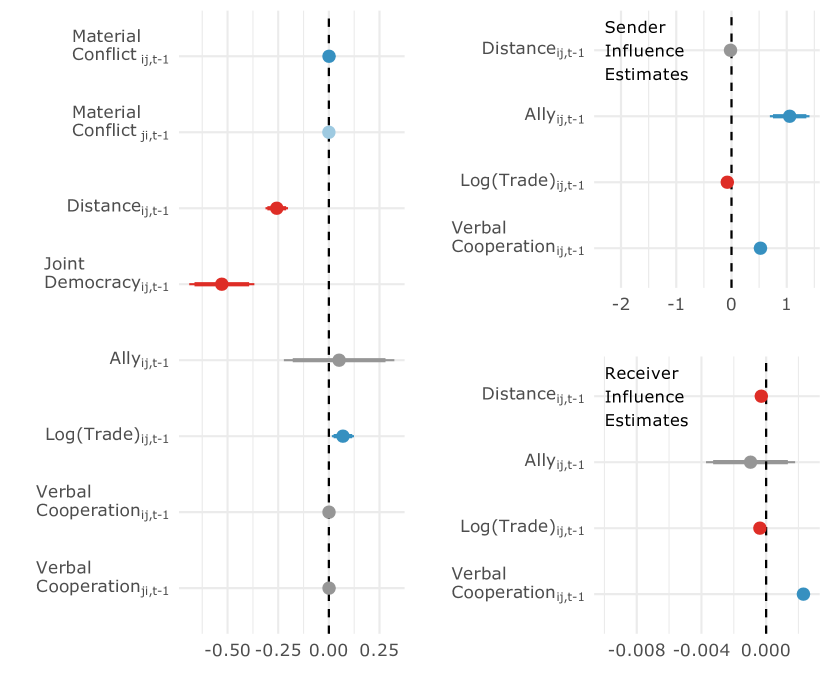
Figure 5. Left-most plot shows results for the direct effect parameters and the top-right plot represents results for the sender influence, and bottom-right receiver influence parameters. Points in each of the plots represents the average effect for the parameter and the width the 90 and 95% confidence intervals. Dark shades of blue and red indicate that the parameter is significant at a 95% confidence interval and lighter shades a 90% confidence interval. Parameters that are not significant are shaded in grey.

The right-most plots focuses what determines sender (top) and receiver (bottom) influence patterns. Interestingly, the alliance sender influence parameter has a positive effect, indicating that countries tend to initiate greater levels of conflict with countries that their allies were fighting in the previous period. This finding is in line with arguments in the extant literature about the role that alliance relationships may play in leading to more conflict in the international system (Siverson and King, 1980; Leeds, 2005).

Additionally, countries are likely to send conflict to those with whom their verbal cooperation partners are initiating or increasing conflict with. This finding is interesting as it highlights that countries making cooperative statements regarding a particular country $i$, actually go beyond those statements in later periods to supporting $i$ by initiating conflict with those that $i$ was in conflict with. Trade flows, on the other hand, are associated with having a negative effect, implying that countries are not likely, and in fact somewhat unlikely, to follow their trading partners into conflict.

Receiver influence patterns are similarly determined. Trade flows and verbal cooperation have similar effects, though the interpretation here for trade is that countries are unlikely to be targeted by those that target their trading partners. Interestingly, the distance effect on the receiver influence side is more precisely measured, implying that geographically proximate countries are more likely to receive conflict from a similar set of countries.

Visualizing Dependence Patterns

Based on the sender and receiver influence parameter estimates, Figure 6 provides a visual summary of the type of dependence patterns that are implied in the context of the material conflict model estimated in the previous section.

The linear combination of our influence parameter estimates ($\alpha$), and the design array containing sender influence variables ($w_{ijt}$) are used to visualize the sender dependence patterns between a pair of countries ($a_{ijt}$): $a_{ijt}=\alpha^{\top}w_{ijt}$. The resulting sender and receiver dependence pattern are shown in Figure 6 for June 2007. For the visualization on the left [right], edges between countries indicate that greater likelihood to send [receive] conflictual events to [from] the same countries. Countries are colored by their relative geographic position and node size corresponds to the number of influence relationships the country shares.

Since these dependence patterns are estimated directly from the model results that are presented in Figure 5, the patterns implied by that model are manifest in these visualizations. One of the more notable findings from the sender influence model is the role that alliance relationships play, and this effect is striking. For example, the USA shares sender influence ties with a number of Western European countries such as Germany and the United Kingdom, the USA also is more likely to send conflict to actors that Australia, South Korea and Japan have engaged in material conflict with, and many of these countries are likely to do the same.

June 2007

Sender Dependence Patterns

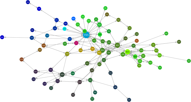
Receiver Dependence Patterns

Figure 6. Network visualization of influence patterns as estimated by the social influence regression model for June 2007. Nodes are colored by their relative geographic position and are sized by the number of influence relationships that they receive and send.

A predictor of receiver influence patterns is the distance between countries. Countries are more likely to be targeted by the same set of countries as their neighbors. This pattern manifests itself in the right-most visualization in Figure 6, where we find clumps of countries, such as Iraq, Lebanon, and Jordan, clustering together.

Performance Comparison

A common and important argument for employing a network based approach is that it aids in better accounting for the data generating process underlying relational data structures.

Thus, in this case, the network approach should actually better predict conflict in an out-of-sample test. To put the performance of this model in context, we compare it to a standard GLM that does not account for dependence patterns in the network, but is similarly parameterized. Additionally, given the recent interest in machine learning methods as tools for prediction within the social sciences we compare the performance against a generalized boosted model (GBM).

Boosting methods have become a popular approach in the machine learning to ensemble over decision tree models in a sequential manner. At each iteration, a new model is trained with respect to the error of the ensemble at that point. Friedman (2001) greatly extended the learning procedure underlying boosting algorithms, by modifying the approach to choose new models at every iteration so that they would be maximally correlated with the negative gradient of some loss function relevant to the ensemble. In the case of a squared-error loss function, this would correspond to sequentially fitting the residuals. We use a generalized version of this model developed by Ridgeway (2012) that extends this framework to the estimation of a variety of distribution types—in our case, a Poisson regression model. In general, these types of models have been shown to give substantial predictive advantage over alternative methods, such as GLM, and should provide a useful point of comparison.

To compare these approaches we first utilize a cross-validation procedure. This involves first randomly dividing $T$ time points in our relational array into $k=10$ sets and within each set we set randomly exclude five time slices from our material conflict array. We then run our models and predict the five missing slices from the estimated parameters. Proper scoring rules are used to compare predictions. Scoring rules evaluate forecasts through the assignment of a numerical score based on the predictive distribution and on the actual value of the dependent variable. Czado, Gneiting and Held (2009) discuss a number of such rules that can be used for count data: Brier, Dawid-Sebastiani, Logarithmic, and Spherical scores. For each of these rules, lower values on the metric indicate better performance.

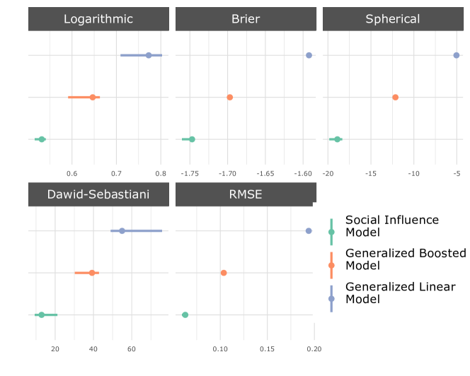
Figure 7. Performance comparison based on randomly excluding time slices from the material conflict array. Colors designate the different models, and the average score across the 10-fold cross validation is designated by a circle and the range by a horizontal line.

Figure 7 illustrates differences in the performance between the social influence model, GLM, and GBM across the scoring rules mentioned above and a more standard metric, the RMSE. In the case of each of these metrics we find GLM performs the worst and that the social influence model performs the best.

Recently, conflict scholars have become interested in generating forecasts from their models (Pevehouse and Goldstein, 1999; de Mesquita, 2009; Brandt, Freeman and Schrodt, 2014; Hegre, Høyland and Nygård, 2015; Ward, 2016). and to assess the performance of their model instead of taking a cross-validation approach they often just predict out some number of years. We perform such an exercise as well by dividing up our sample into a training and test set, where the test set corresponds to the last $x$ periods in the data that we have available. We vary $x$ from two to five. For instance, when $x=5$ we are leaving the last five years of data for validation. Results for this analysis are shown in Figure 8 and there again we find that the social influence model has better out of sample predictive performance than the alternatives we test here.

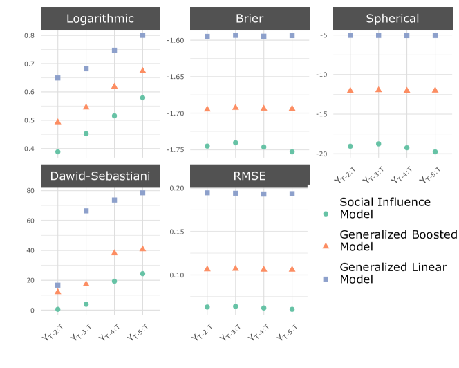
Figure 8. Performance comparison based on randomly excluding the last two to five periods of the material conflict array. Colors and shapes designate the different models, and the score when excluding $x$ number of periods is shown.

Conclusion

Both measuring influence and determining the drivers of it are topics of perennial interest in network analysis and political science. Within political science, determining whether and how actors within relational systems influence one another is a topic of particular interest in regards to deriving measures surrounding the relative “power” of states. Though much past work has drawn upon explanations based on power to assess world events, extant operationalizations of this concept can be improved.

The standard approach of assessing the relative power of a pair of states is derived by calculating the ratio of their material capabilities (e.g., Slantchev 2004; Reed et al. 2008; Butler and Gates 2009; Gartzke and Weisiger 2014). The availability of quantitative data on material characteristics of states (e.g., population, iron and steel production, military size) was to influence greatly the scholarship in this area. Currently, many scholars continue to rely on indices such as the Correlates of War’s Composite Index of National Capabilities (CINC) as a way of assessing power (Singer, Bremer and Stuckey, 1972). For the most part, this has pushed scholarly consideration of power into a capabilities direction, rather than a direction in which power was seen as relational.

These approaches have implicitly assumed that power is material and fungible. If China has more capabilities than India, it has more power. If India and Japan together have more capabilities than China, then they have more power. Yet, relying on these types of measures ignores the nuances of regional as well as global interactions, and disregards the contexts in which states interact. Further, the narrow interpretation of power characterized by purely detracts from a more relevant question regarding relational data, namely, how do the actions of actors within a network influence the actions of others. Through using the approach we have introduced here scholars can continue to test theories regarding the role that alliances or trade flows may play in influencing states, but can move towards doing so within a network context.

The work that we have done is also relevant for the networks literature. Discussions around measurements of influence often begin and end with the use of various centrality measures. Yet, centrality measures just provide a representation of how “important” a node is within a network, and do not detail how a pair of nodes might be influencing the actions of one another. Further centrality measures for the most part are just descriptive tools. Of course one can shift towards using alternative approaches such as latent variable models, but these approaches cast little light on exogenous attributes that might be shaping how actors within a system influence one another in a longitudinal context. The approach that we introduce here is an extension of earlier work involving the bilinear autoregression model, and we have now simplified it into a rank one regression model. This approach allows us to estimate the role that nodal and dyadic attributes may play in how dyads influence one another, and because this approach is estimated within a GLM framework it is readily extendable to a variety of other settings.

Appendix

Visualization of convergence for direct (blue), sender influence (green), and receiver influence (red) parameters.

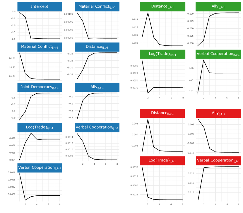
Figure A1. Convergence diagnostics for the social influence regression model on material conflict.

Convergence

Influence Dynamics

Visualization of influence effects for select time points from dynamic social influence regression model.

Sender Influence Space:
February 2005	September 2006	June 2007
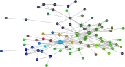
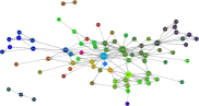
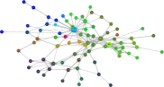
April 2008	January 2009	August 2010
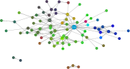
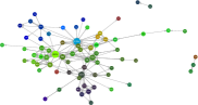
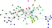
October 2009	May 2011	December 2012
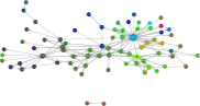
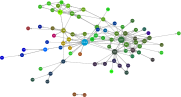
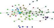
Receiver Influence Space:
February 2005	September 2006	June 2007
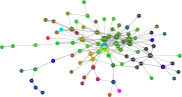
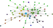
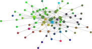
April 2008	January 2009	August 2010
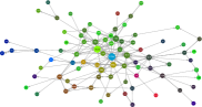
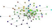
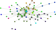
October 2009	May 2011	December 2012

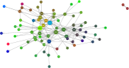
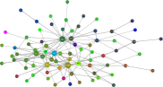
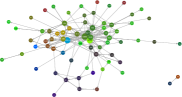
Figure A2. Influence relationships

Scoring Rules for Count Data

Scoring rules are penalties $s(y,P)$ introduced with $P$ being the predictive distribution and $y$ the observed value. The goal of researchers interested in prediction is to minimize the expectation of these scores, which is typically calculated by taking the average:

$S=\frac{1}{n}\sum_{i=1}^{n}s(y_{i},P_{i}),$

where $y_{i}$ refers to the $i^{th}$ observed count and $P_{i}$ the $i^{th}$ predictive distribution. A set of proper scoring rules as defined by Czado, Gneiting and Held (2009) are shown in the list below. For each of these rules, $f(y)$ denotes the predictive probability mass function. $\hat{\mu}$ and $\hat{\sigma}$ refer to the mean and standard deviation of the predictive distribution.

• Dawid-Sebastiani score: $s(y,P)=(\frac{y-\hat{\mu}}{\hat{\sigma}})^{2}+2\times log(\hat{\sigma})$

• Logarithmic score: $s(y,P)=-log(f(y))$

• Brier score: $s(y,P)=-2f(y)+\sum_{k}f^{2}(k)$

• Spherical score: $s(y,P)=\frac{f(y}{\sqrt{\sum_{k}f^{2}(k)}}$

References

- (1)
- Baldwin (1978) Baldwin, David A. 1978. “Power and Social Exchange.” American Political Science Review 72:1229–1242.
- Barbieri (1996) Barbieri, Katherine. 1996. “Economic interdependence: A path to peace or a source of interstate conflict?” Journal of Peace Research 33(1):29–49.
- Barnett and Duvall (2004) Barnett, Michael and Raymond Duvall. 2004. Power in global governance. Vol. 98 New York: Cambridge University Press.
- Boschee et al. (2015a) Boschee, Elizabeth, Jennifer Lautenschlager, Sean O’Brien, Steve Shellman, James Starz and Michael D. Ward. 2015a. “ICEWS Coded Event Data.” http://dx.doi.org/10.7910/DVN/28075 Harvard Dataverse Network [Distributor] V1 [Version].
- Boschee et al. (2015b) Boschee, Elizabeth, Jennifer Lautenschlager, Sean O’Brien, Steve Shellman, James Starz and Michael D. Ward. 2015b. “ICEWS Coded Event Data.” Harvard Dataverse Network (http://dx.doi.org/10.7910/DVN/28075).
- Boschee, Natarjan and Weischedel (2013) Boschee, Elizabeth, Premkumar Natarjan and Ralph Weischedel. 2013. Automatic Extraction of Events from Open Source Text for Predictive Forecasting. In Handbook of Computational Approaches to Counterterrorism, ed. Venkatramana S. Subrahmanian. New York: Springer.
- Brandt, Freeman and Schrodt (2014) Brandt, Patrick T., John R. Freeman and Philip A. Schrodt. 2014. “Evaluating Forecasts of Political Conflict Dynamics.” International Journal of Forecasting 30(4):944–962.
- Brandt et al. (2000) Brandt, Patrick T, John T Williams, Benjamin O Fordham and Brain Pollins. 2000. “Dynamic modeling for persistent event-count time series.” American Journal of Political Science pp. 823–843.
- Bremer (1992) Bremer, Stuart A. 1992. “Dangerous dyads conditions affecting the likelihood of interstate war, 1816-1965.” Journal of Conflict Resolution 36(2):309–341.
- Butler and Gates (2009) Butler, Christopher and Scott Gates. 2009. “Asymmetry, Parity, and (Civil) War: Can International Theories of Power Help Us Understand Civil War?” International Interactions 35(3):330–340.
- Carter and Goemans (2011) Carter, David B. and Hein E Goemans. 2011. “The Making of the Territorial Order: New Borders and the Emergence of Interstate Conflict.” International Organization 65(02):275–309.
- Cho and Fowler (2010) Cho, Wendy K. Tam and James H. Fowler. 2010. “Legislative success in a small world: Social network analysis and the dynamics of congressional legislation.” The Journal of Politics 72(01):124–135.
- Choucri and North (1972) Choucri, Nazli and Robert C. North. 1972. “Dynamics of International Conflict.” World Politics 24(2):80–122.
- Czado, Gneiting and Held (2009) Czado, Claudia, Tilmann Gneiting and Leonhard Held. 2009. “Predictive Model Assessment for Count Data.” Biometrics 65(4):1254–1261.
- de Bie et al. (2017) de Bie, Jasper L., Christianne J. de Poot, Joshua D. Freilich and Steven M. Chermak. 2017. “Changing organizational structures of jihadist networks in the Netherlands.” Social Networks 48:270–283.
- de Mesquita (2009) de Mesquita, Bruce Bueno. 2009. The Predictioneer’s Game. New York, NY: Random House.
- Diehl and Goertz (2000) Diehl, Paul F. and Gary Goertz. 2000. War and peace in international rivalry. Ann Arbor, MI: University of Michigan Press.
- Doran and Parsons (1980) Doran, Charles F. and Wes Parsons. 1980. “War and the Cycle of Relative Power.” American Political Science Review 74(4):997–965.
- Duval and Thompson (1980) Duval, Robert D. and William R. Thompson. 1980. “Reconsidering the aggregate relationship between size, economic development, and some types of foreign policy behavior.” American Journal of Political Science pp. 511–525.
- Fearon (1995) Fearon, James D. 1995. “Rationalist Explanations for War.” International Organization 49(3):379–414.
- Friedman (2001) Friedman, Jerome H. 2001. “Greedy function approximation: A gradient boosting machine.” Annals of statistics pp. 1189–1232.
- Fucks (1965) Fucks, Wilhelm. 1965. Formeln zur Macht: Prognosen uber Volker, Wirtschafte, Potentiale. Stuttgart: Duetsche Verlags-Anstalt.
- Gartzke and Weisiger (2014) Gartzke, Erik and Alex Weisiger. 2014. “Under Construction: Development, Democracy, and Difference as Determinants of Systemic Liberal Peace.” International Studies Quarterly 58(1):130–145.
- Gartzke, Li and Boehmer (2001) Gartzke, Erik, Quan Li and Charles Boehmer. 2001. “Investing in the Peace: Economic Interdependence and International Conflict.” International Organization 55(2):391–438.
- Gibler and Sarkees (2004) Gibler, Douglas M. and Meredith Sarkees. 2004. “Measuring Alliances: the Correlates of War Formal Interstate Alliance Data Set, 1816-2000.” Journal of Peace Research 41(2):211–222.
- Goldstein (1992) Goldstein, Joshua. 1992. “A Conflict-Cooperation Scale for WEIS International Events Data.” Journal of Conflict Resolution 36(2):369–385.
- Gowa and Mansfield (1993) Gowa, Joanne and Edward D. Mansfield. 1993. “Power Politics and International Trade.” American Political Science Review 87(2):408–420.
- Haas (1953) Haas, Ernst B. 1953. “The balance of power: prescription, concept, or propaganda?” World Politics 5(04):442–477.
- Hegre, Høyland and Nygård (2015) Hegre, Håvard, Bjørn Høyland and Håvard Nygård. 2015. “Dynamic Prediction of Armed Conflict, 2015—2065.” Peace Research Institute Oslo Conference: Early Warning: Forecasting and Early Warning of Conflict.
- Hoff (2005) Hoff, Peter D. 2005. “Bilinear Mixed-Effects Models for Dyadic Data.” Journal of the American Statistical Association 100(4690):286–295.
- Hoff (2015) Hoff, Peter D. 2015. “Multilinear Tensor Regression for Longitudinal Relational Data.” The Annals of Applied Statistics 9(3):1169–1193.
- Hoff, Raftery and Handcock (2002) Hoff, Peter D., Adrian E. Raftery and Mark S. Handcock. 2002. “Latent space approaches to social network analysis.” Journal of the American Statistical Association 97(460):1090–1098.
- International Monetary Fund (2012) International Monetary Fund. 2012. “IMF eLibrary Data.” http://elibrary-data.imf.org (accessed July 19, 2012).
- Izenman (1975) Izenman, Alan Julian. 1975. “Reduced-rank regression for the multivariate linear model.” Journal of Multivariate Analysis 5(2):248–264.
- Kadera (2001) Kadera, Kelly M. 2001. The Power-Conflict Story: A Dynamic Model of Interstate Rivalry. Ann Arbor, MI, USA: University of Michigan Press.
- Keohane and Nye (1977) Keohane, Robert and Joseph Nye. 1977. Power and Interdependence: World Politics in Transition. Boston, MA: Little Brown.
- Keohane (1989) Keohane, Robert O. 1989. “Reciprocity in international relations.” International Organization 40(1).
- Krivitsky and Handcock (2014) Krivitsky, Pavel N. and Mark S. Handcock. 2014. “A separable model for dynamic networks.” Journal of the Royal Statistical Society: Series B (Statistical Methodology) 76(1):29–46.
- Lautenschlager, Shellman and Ward (2015) Lautenschlager, Jennifer, Steve Shellman and Michael D. Ward. 2015. “ICEWS Coded Event Aggregations.” http://dx.doi.org/10.7910/DVN/28117 Harvard Dataverse Network [Distributor] V1 [Version].
- Leeds (2005) Leeds, Brett A. 2005. Alliances and the expansion and escalation of militarized interstate disputes. In New Directions in International Relations. Lanham: Lexington Books pp. 117–34.
- Leeds (2003) Leeds, Brett Ashley. 2003. “Do alliances deter aggression? The influence of military alliances on the initiation of militarized interstate disputes.” American Journal of Political Science 47(3):427–439.
- Li, Kim and Altman (2010) Li, Bing, Min Kyung Kim and Naomi Altman. 2010. “On dimension folding of matrix-or array-valued statistical objects.” The Annals of Statistics pp. 1094–1121.
- Livi et al. (2016) Livi, Lorenzo, Enrico Maiorino, Alessandro Giuliani, Antonello Rizzi and Alireza Sadeghian. 2016. “A generative model for protein contact networks.” Journal of Biomolecular Structure and Dynamics 34(7):1441–1454.
- Maoz and Russett (1993) Maoz, Zeev and Bruce M. Russett. 1993. “Normative and Structural Causes of Democratic Peace, 1946-1986.” American Political Science Review 87(3):624–38.
- Maoz and Abdolali (1989) Maoz, Zeev and Nasrin Abdolali. 1989. “Regime Types and International Conflict, 1816-1976.” Journal of Conflict Resolution 33(1):3–35.
- Marshall and Jaggers (2002) Marshall, Monty G. and Keith Jaggers. 2002. “Polity IV Project: Political Regime Characteristics and Transitions, 1800-2002, Dataset Users’ Manual.” Center for International Development and Conflict Management, University of Maryland.
- Metternich, Minhas and Ward (2015) Metternich, Nils, Shahryar Minhas and Michael Ward. 2015. “Firewall? or Wall on Fire? A Unified Framework of Conflict Contagion and the Role of Ethnic Exclusion.” Journal of Conflict Resolution Online version(doi:10.1177/0022002715603452).
- Minhas, Hoff and Ward (2016) Minhas, Shahryar, Peter D. Hoff and Michael D. Ward. 2016. “A New Approach to Analyzing Coevolving Longitudinal Networks in International Relations.” Journal of Peace Research 53(3):491–505.
- Nexon (2009) Nexon, Daniel H. 2009. The Struggle for Power in Early Modern Europe: Religion Conflict, Dynastic Empires, and International Change. Princeton, N.J.: Princeton University Press.
-
OEDA (2016)
OEDA. 2016.
“Open Event Data Alliance: Phoenix Data Base.”.
http://phoenixdata.org/ - Pevehouse and Goldstein (1999) Pevehouse, Jon C. and Joshua S. Goldstein. 1999. “Serbian compliance or defiance in Kosovo? Statistical analysis and real-time predictions.” The Journal of Conflict Resolution 43(4):538–546.
- Rajmaira and Ward (1990) Rajmaira, Sheen and Michael D. Ward. 1990. “Evolving Foreign Policy Norms: Reciprocity in the Superpower Triad.” International Studies Quarterly 34:457–475.
- Reed et al. (2008) Reed, William, David H. Clark, Timothy Nordstrom and Wonjae Hwang. 2008. “War, Power, and Bargaining.” The Journal of Politics 70(04):1203–1216.
- Richardson (1960) Richardson, Lewis F. 1960. Arms and Insecurity. Chicago and Pittsburgh, PA: Quadrangle/Boxwood.
-
Ridgeway (2012)
Ridgeway, Greg. 2012.
“Generalized Boosted Models: A guide to the gbm package.”.
https://github.com/harrysouthworth/gbm/blob/master/inst/doc/gbm.pdf - Rummel (1979) Rummel, Rudolph J. 1979. War, Power, Peace. Vol. 4 of Understanding Conflict and War Sage.
- Russett and Oneal (2001) Russett, Bruce M. and John Oneal. 2001. Triangulating Peace: Democracy, Interdependence, and International Organizations. New York: W.W. Norton.
- Schein et al. (2015) Schein, Aaron, John Paisley, David M. Blei and Hanna Wallach. 2015. Bayesian poisson tensor factorization for inferring multilateral relations from sparse dyadic event counts. In Proceedings of the 21th ACM SIGKDD International Conference on Knowledge Discovery and Data Mining. ACM pp. 1045–1054.
- Schrodt, Gerner and Yilmaz (2009) Schrodt, Philip A., Debora J. Gerner and Omur Yilmaz. 2009. Conflict and Mediation Event Observations (CAMEO): An Event Data Framework for a Post Cold War World. In International Conflict Mediation: New Approaches and Findings, ed. Jacob Bercovitch and Scott Sigmund Gartner. New York: Routledge.
- Schrodt and Yonamine (2013) Schrodt, Philip A. and James E. Yonamine. 2013. “A Guide to Event Data: Past, Present, and Future.” All Azimuth 2(2):5.
- Sewell and Chen (2015) Sewell, Daniel K. and Yuguo Chen. 2015. “Latent space models for dynamic networks.” Journal of the American Statistical Association 110(512):1646–1657.
- Singer, Bremer and Stuckey (1972) Singer, J. David, Stuart A. Bremer and John Stuckey. 1972. Capabiity Distribution, Uncertainty, and Major Power War, 1820-1965. In Peace, War, and Numbers, ed. Bruce M. Russett. 1st ed. Beverly Hills, CA: Sage Publishers chapter 1, pp. 19–48.
- Siverson and King (1980) Siverson, Randolph M. and Joel King. 1980. “Attributes of national alliance membership and war participation, 1815-1965.” American Journal of Political Science pp. 1–15.
- Slantchev (2004) Slantchev, Branislav L. 2004. “How Initiators End Their Wars: The Duration of Warfare and the Terms of Peace.” American Journal of Political Science 48(4):813–829.
- Small and Singer (1976) Small, Melvin and J. David Singer. 1976. “The War Proneness of Democratic Regimes.” Jerusalem Journal of International Relations 1(1):49–69.
- Snijders (2014) Snijders, Tom A.B. 2014. Siena: Statistical Modeling of Longitudinal Network Data. In Encyclopedia of Social Network Analysis and Mining. Springer New York pp. 1718–1725.
- Snijders and Nowicki (1997) Snijders, Tom A.B. and Krzysztof Nowicki. 1997. “Estimation and prediction for stochastic blockmodels for graphs with latent block structure.” Journal of Classification 14(1):75–100.
- Snyder (1984) Snyder, Glenn H. 1984. “The security dilemma in alliance politics.” World politics 36(4):461–495.
- Vasquez and Rundlett (2016) Vasquez, John A. and Ashlea Rundlett. 2016. “Alliances as a Necessary Condition of Multiparty Wars.” Journal of Conflict Resolution 60(8):1395–1418.
- Von Clausewitz (1832) Von Clausewitz, Carl. 1832. Vom Kriege: Hinterlassenes Werk. Berlin: Fredinand Dümmler.
- Waltz (1979) Waltz, Kenneth N. 1979. Theory of International Politics. Reading: Addison-Wesley.
- Ward (2016) Ward, Michael D. 2016. “Can We Predict Politics? Toward What End?” Journal of Global Security Studies 1(1):80–91.
- Weidmann, Kuse and Gleditsch (2010) Weidmann, Nils B., Doreen Kuse and Kristian Skrede Gleditsch. 2010. “The Geography of the International System: The CShapes Dataset.” International Interactions 36(1):86–106.
- Welch, Bansal and Hunter (2011) Welch, David, Shweta Bansal and David R. Hunter. 2011. “Statistical inference to advance network models in epidemiology.” Epidemics 3(1):38–45.
- Wu et al. (2009) Wu, Jianmin, Tea Vallenius, Kristian Ovaska, Jukka Westermarck, Tomi P Mäkelä and Sampsa Hautaniemi. 2009. “Integrated network analysis platform for protein-protein interactions.” Nature Methods 6(1):75–77.
- Zhou, Li and Zhu (2013) Zhou, Hua, Lexin Li and Hongtu Zhu. 2013. “Tensor regression with applications in neuroimaging data analysis.” Journal of the American Statistical Association 108(502):540–552.