Structured Recommendation

Abstract

Current recommender systems largely focus on static, unstructured content. In many scenarios, we would like to recommend content that has structure, such as a trajectory of points-of-interests in a city, or a playlist of songs. Dubbed Structured Recommendation, this problem differs from the typical structured prediction problem in that there are multiple correct answers for a given input. Motivated by trajectory recommendation, we focus on sequential structures but in contrast to classical Viterbi decoding we require that valid predictions are sequences with no repeated elements. We propose an approach to sequence recommendation based on the structured support vector machine. For prediction, we modify the inference procedure to avoid predicting loops in the sequence. For training, we modify the objective function to account for the existence of multiple ground truths for a given input. We also modify the loss-augmented inference procedure to exclude the known ground truths. Experiments on real-world trajectory recommendation datasets show the benefits of our approach over existing, non-structured recommendation approaches.

1 Introduction

Content recommendation has been the subject of a rich body of literature [1, 2, 3], with established techniques seeing widespread adoption in industry [4, 5, 6, 7]. The success of these methods is explained by both the explosion in availability of user’s explicit and implicit preferences for content, as well as the design of methods that can suitably exploit these to make useful recommendations [8].

Classical recommendation systems have focused on a fixed set of individual items such as movies, dubbed here as recommending unstructured content. While this setting has considerable value, in many important scenarios one needs to recommend content that possesses some structure. An example of this is where the desired content is naturally organized in sequences or graphs. For example, consider recommending a trajectory of points of interest in a city to a visitor [9, 10, 11, 12], a playlist of songs [13, 14, 15, 16], a chemical compound [17] or a few linked websites for e-commerce [18].

A naïve approach to sequence recommendation is to ignore the structure. In the trajectory example, we could learn a user’s preference for individual locations, and create a trajectory based on the top ranked locations. However, such an approach may be sub-optimal: for example, in the trajectory recommendation problem, it is unlikely a user will want to visit three restaurants in a row. Similarly, while a user’s two favourite songs might belong the metal and country genres respectively, it is questionable that a playlist featuring these songs in succession will be as enjoyable to the user.

The above raises the question of how one can effectively learn from such sequential content. In this paper, we show how to cast sequence recommendation as a structured prediction problem, which allows us to leverage the toolkit of structured SVMs [19]. However, a vanilla application of such methods does not suffice, as they do not account for the fact that each input can have multiple ground truths, and that repeated elements in predicted sequences are undesirable. We show how to overcome this by incorporating multiple correct sequences into a structured prediction formulation, and by two novel applications of the list Viterbi algorithm that sequentially finds the list of top-scoring sequences. Specifically, our contributions are as follows:

• We formalise the problem of sequence recommendation (§2.1), and show how trajectory recommendation can be seen as a special case (§2.3).

• We show how sequence recommendation may be attacked using structured SVMs (§3). We propose one improvement of structured SVMs to the recommendation problem, so as to account for the existence of multiple ground truths for each input (§3.2).

• We propose two novel applications of the list Viterbi algorithm – an extension of the classic Viterbi algorithm that sequentially finds the list of highest scored sequences under some model – to exclude multiple ground truths for model learning (§3.3), and to predict sequences without repeated elements, i.e. paths in state-space (§3.4).

• We present experiments on real-world trajectory recommendation problems, and demonstrate our structured recommendation approaches improve over existing non-structured baselines (§4).

2 The structured recommendation problem

We introduce the structured recommendation problem that is the focus of this paper. We then provide some motivating examples, in particular the problem of trajectory recommendation.

2.1 Structured and sequence recommendation

Consider the following general structured recommendation problem: given an input query $\mathbf{x}\in\mathcal{X}$ (representing e.g. a location, or some “seed” song) we wish to recommend one or more structured outputs $\mathbf{y}\in\mathcal{Y}$ (representing e.g. a sequence of locations, or songs) according to a learned score function $f(\mathbf{x},\mathbf{y})$. To learn $f$, we are provided as input a training set $\{(\mathbf{x}^{({i})},\{\mathbf{y}^{({ij})}\}_{j=1}^{n_{i}})\}_{i=1}^{n}$, comprising a collection of inputs $\mathbf{x}^{({i})}$ with an associated set of $n_{i}$ output structures $\{\mathbf{y}^{({ij})}\}_{j=1}^{n_{i}}$.

For this work, we assume the output $\mathbf{y}$ is a sequence of $l$ points, denoted $y_{1:l}$ where each $y_{i}$ belongs to some fixed set (e.g. places of interest in a city, or a collection of songs). We call the resulting specialisation the sequence recommendation problem, and this shall be our primary interest in this paper. In many settings, one further requires the sequences to be paths, i.e. not contain any repetitions.

As a remark, we note that the assumption that $\mathbf{y}$ is a sequence does not limit the generality of our approach, as inferring $\mathbf{y}$ of other structures can be achieved using corresponding inference and loss-augmented inference algorithms [20].

2.2 Sequence recommendation versus existing problems

There are key differences between sequence recommendation and standard problems in structured prediction and recommender systems; this brings unique challenges for both inference and learning.

In a structured prediction problem (for sequences), the goal is to learn from a set of input vector and output sequence tuples $\{(\mathbf{x}^{({i})},\mathbf{y}^{({i})})\}_{i=1}^{n}$, where for each input $\mathbf{x}^{({i})}$ there is usually one unique output sequence $\mathbf{y}^{({i})}$. In a sequence recommendation problem, however, we expect that for each input $\mathbf{x}^{({i})}$ (e.g. users), there are multiple associated outputs $\{\mathbf{y}^{({ij})}\}_{j=1}^{n_{i}}$ (e.g. trajectories visited). Structured prediction approaches do not have a standard way to handle such multiple output sequences. Furthermore, it is desirable for the recommended sequence to consist of unique elements, or be a path [21] in the candidate space (e.g. locations). Classic structured prediction does not constrain the output sequence, and having such a path constraint makes both inference and learning harder.

In a typical recommender systems problem, the outputs are non-structured; canonically, one works with static content such as books or movies [1, 2, 22]. Thus, making a prediction involves enumerating all non-structured items $y$ in order to compute $\operatorname*{argmax}_{y}f(\mathbf{x},y)$ for suitable score function $f$, e.g. some form of matrix factorisation [8]. For sequence recommendation, computing $\operatorname*{argmax}_{\mathbf{y}}f(\mathbf{x},\mathbf{y})$ is harder since it is often impossible to efficiently enumerate $\mathbf{y}$ (e.g. all possible trajectories in a city). This inability to enumerate $\mathbf{y}$ also poses a challenge in designing a suitable $f(\mathbf{x},\mathbf{y})$, e.g. matrix factorisation would require associating a latent feature with each $\mathbf{y}$, which will be infeasible.

2.3 Examples of sequence recommendation

To make the sequence recommendation problem more concrete, we provide three specific examples, starting with the problem of trajectory recommendation that shall serve as a recurring motivation. Note that in all these problems, one is specifically interested in sequences that are paths.

Trajectory recommendation. Travel recommendation problems involve a set of points-of-interest (POIs) $\mathcal{P}$ in a city [23, 24, 25]. Given a trajectory query $\mathbf{x}=(s,l)$, comprising a start POI $s\in\mathcal{P}$ and trip length $l\!>\!1$ (i.e. the desired number of POIs, including $s$), the trajectory recommendation problem is to recommend one or more sequences of POIs that maximise some notion of utility, learned from a training set of trajectories visited by travellers in the city.

Existing approaches treat the problem as one of determining a score for the intrinsic appeal of each POI. For example, a RankSVM model which learns to predict whether a POI is likely to appear ahead of another POI in a trajectory corresponding to some query [12]. Formally, from the given set of trajectories we derive a training set $\{(\mathbf{x}^{(i)},\mathbf{r}^{(i)})\}_{i=1}^{n}$, where for each trajectory query $\mathbf{x}^{(i)}$ there is a list of ranked POI pairs $\mathbf{r}^{(i)}\subseteq\mathcal{P}\times\mathcal{P}$ such that $(p,p^{\prime})\in\mathbf{r}^{(i)}$ iff POI $p$ appears more times than POI $p^{\prime}$ in all trajectories associated with $\mathbf{x}^{(i)}$. The training objective is then

(1)

for feature mapping $\Psi$, regularisation strength $C$ and squared hinge loss $\ell(v)=\max(0,1-v)^{2}$.

We can view trajectory recommendation as sequence recommendation in the following way: given trajectory query $\mathbf{x}$, and a suitable scoring function $f$, we wish to find $\mathbf{y}^{*}=\operatorname*{argmax}_{\mathbf{y}\in\mathcal{Y}}~{}f(\mathbf{x},\mathbf{y}),$ where $\mathcal{Y}$ is the set of all possible trajectories with POIs in $\mathcal{P}$ that conform to the constraints imposed by the query $\mathbf{x}$. In particular, $\mathbf{y}=(s,~{}y_{2},\dots,y_{l})$ is a trajectory with $l$ POIs. This was the view proposed in [12] where they authors considered an objective function that added two components together: a POI score and a transition score.

Now, our training set of historical trajectories may be written as $\{(\mathbf{x}^{({i})},\{\mathbf{y}^{({ij})}\}_{j=1}^{n_{i}})\}_{i=1}^{n}$, where each $\mathbf{x}^{({i})}$ is a distinct query with $\{\mathbf{y}^{({ij})}\}_{j=1}^{n_{i}}$ the corresponding set of observed trajectories. Note that we expect most queries to have several distinct trajectories; minimally, for example, there may be two nearby POIs that are visited in interchangeable order by different travellers. We are also interested in predicting paths $\mathbf{y}$, since it is unlikely a user will want to visit the same location twice.

Playlist generation. As another example, consider recommending song playlists (i.e. sequences) to users, given a query song [13, 14, 15, 16]. A canonical approach is to learn a latent representation of songs from historical playlists, and exploit a Markovian assumption on the song transitions.

Next basket and next song prediction. One more example of sequence recommendation is the problem of recommending the next items a user might like to purchase, given the sequence of their shopping basket purchases [26, 27]. The canonical approach here is to apply matrix factorisation to the Markov chain of transitions between items. This method is feasible because one is only interested in predicting sequences one element at a time, instead of predicting the entire sequence given the initial item. Recent approaches using recurrent neural networks for next basket prediction [28] and playlist generation [16] also focus on modelling high quality transitions only.

2.4 The case for exploiting structure

Each of the sequence recommendation problems above can be plausibly solved with approaches that do not exploit the structure inherent in the outputs $\mathbf{y}$. While such approaches can certainly be useful, their modelling power is inherently limited, as they cannot ensure the global cohesion of the corresponding recommendations $\mathbf{y}$. For example, in the trajectory recommendation problem, the RankSVM model might find three restaurants to be the highest scoring POIs; however, it is unlikely that these form a trajectory that most travellers will enjoy.

This motivates an approach to sequence recommendation that directly ensures such global cohesion. We now see how to do so with novel extensions to structured prediction approaches.

3 A structured prediction approach to sequence recommendation

We now describe a method to solve sequence recommendation problems. We first provide background on structured SVMs (SSVM) (Sec 3.1), then present a model for structured recommendation (Sec 3.2), followed by the correspondingly updated algorithms for its learning (Sec 3.3) and inference (Sec 3.4).

3.1 Background: SSVM for structured prediction

A structured prediction task involves predicting some structured label $\mathbf{y}\in\mathcal{Y}$ for an input $\mathbf{x}\in\mathcal{X}$, typically via a score function $f(\mathbf{x},\mathbf{y})$ that determines the affinity of an (input, label) pair. A popular model is the Structured Support Vector Machine (SSVM) [20, 19], comprising three core ingredients.

Score function. In SSVMs, we specify that the score function $f(\mathbf{x},\mathbf{y})$ takes a linear form, i.e. $f(\mathbf{x},\mathbf{y})=\mathbf{w}^{\top}\Psi(\mathbf{x},\mathbf{y})$, where $\mathbf{w}$ is a weight vector, and $\Psi(\mathbf{x},\mathbf{y})$ is a joint feature map.

The design of the feature map $\Psi$ is problem specific. For sequence prediction problems, consider the unary terms for each element in the label $y_{1:l}$, and pairwise interactions between adjacent elements in the label, i.e. $y_{j}$ and $y_{j+1}$ for $j=1:l\!-\!1$. Subsequently, $f(\mathbf{x},\mathbf{y})$ decomposes into a weighted sum of each of these features:

$$f(\mathbf{x},\mathbf{y})=\mathbf{w}^{\top}\Psi(\mathbf{x},\mathbf{y})=\sum_{j=1}^{l}\mathbf{w}_{j}^{\top}\psi_{j}(\mathbf{x},y_{j})+\sum_{j=1}^{l-1}\mathbf{w}_{j,j+1}^{\top}\psi_{j,j+1}(\mathbf{x},y_{j},y_{j+1}).\vspace{-1.0mm}$$ (2)

Here, $\psi_{j}$ is a feature map between the input and one output label element $y_{j}$, with a corresponding weight vector $\mathbf{w}_{j}$, and $\psi_{j,j+1}$ is a pairwise feature vector that captures the interactions between consecutive labels $y_{j}$ and $y_{j+1}$, with a corresponding weight vector $\mathbf{w}_{j,j+1}$.

Objective function. To learn a suitable weight vector $\mathbf{w}$, SSVMs solve:

Here, $\mathcal{Y}$ is the set of all possible sequences and $\Delta(\mathbf{y}^{({i})},\bar{\mathbf{y}})$ is the loss function between $\bar{\mathbf{y}}$ and the ground truth $\mathbf{y}^{({i})}$, and slack variable $\xi_{i}$ is the hinge loss for the prediction of the $i$-th example [19]. Alternatively, we can use one slack variable to represent the sum of the $n$ hinge losses in (3), i.e. the 1-slack formulation [19].

Loss-augmented inference. We can rewrite the constraints in (3) as $\mathbf{w}^{\top}\Psi(\mathbf{x}^{({i})},\mathbf{y}^{({i})})+\xi_{i}\geq\max_{\bar{\mathbf{y}}\in\mathcal{Y}}\left\{\Delta(\mathbf{y}^{({i})},\bar{\mathbf{y}})+\mathbf{w}^{\top}\Psi(\mathbf{x}^{({i})},\bar{\mathbf{y}})\right\}$, and the maximisation at the right side is known as the loss-augmented inference. When the underlying graph of SSVM is a tree (which is the case for sequence recommendation), this may be done efficiently if the loss function $\Delta(\cdot,\cdot)$ is decomposable with respect to individual and pairs of label elements, e.g. using the Viterbi algorithm [20].

3.2 SSVM for structured recommendation: the SP and SR models

We now present two possible means of applying SSVMs to sequence recommendation.

The SP model. Recall that structured recommendation involves observing multiple ground truth outputs for each input, i.e. for input $\mathbf{x}^{({i})}$, there is a set of ground truths $\{\mathbf{y}^{({ij})}\}_{j=1}^{n_{i}}$. One naïve approach to the problem is creating $n_{i}$ examples $\{(\mathbf{x}^{({i})},\mathbf{y}^{({ij})})\}_{j=1}^{n_{i}}$, and feeding this to the classic SSVM. We call this the structured prediction (SP) model.

The SP model is appealing due to its simplicity. However, it is sub-optimal: the result of loss-augmented inference on $(\mathbf{x}^{({i})},\mathbf{y}^{({ij})})$ could be a ground truth label $\mathbf{y}^{\prime}\in\{\mathbf{y}^{({ij})}\}_{j=1}^{n_{i}}$, which means we would incorrectly penalise predicting $\mathbf{y}^{\prime}$ for $\mathbf{x}^{({i})}$.

The SR model. To overcome the limitation of the SP model, we propose the following structured recommendation (SR) model that extends the SSVM to explicitly incorporate multiple ground truths:

where $N=\sum_{i}n_{i}$ and $\bar{\mathbf{y}}^{(i)}\in\mathcal{Y}\setminus\{\mathbf{y}^{(ij)}\}_{j=1}^{n_{i}}$. The 1-slack formulation of (4) can be formed similar to that of (3). Intuitively, the objective in (4) is similar to a ranking objective, as the constraints enforce that the positively labeled sequences (the known items that the user likes) are scored higher than all other unseen sequences. Such objectives have been proven useful in classic unstructured recommendation [29].

Compared to the SP model (3), the key distinction is that (4) explicitly aggregates all the ground truth sequences for each input when generating the constraints, i.e. the loss-augmented inference becomes

$$\max_{\bar{\mathbf{y}}^{(i)}\in\ \mathcal{Y}\setminus\{\mathbf{y}^{(ij)}\}_{j=1}^{n_{i}}}\left(\Delta(\mathbf{y}^{(ij)},\bar{\mathbf{y}}^{(i)})+\mathbf{w}^{\top}\Psi(\mathbf{x}^{(i)},\bar{\mathbf{y}}^{(i)})\right).$$ (5)

In this way, we do not have contradictory constraints where two ground truth sequences are each required to have larger score than the other.

The SP and SR models can be learned using a rich set of training schemes such as cutting-plane algorithms [20], gradient-based algorithms [30] and conditional gradient methods [31] giving proper loss augmented inference and prediction procedures, which we describe in the next two sections.

Beyond dealing with multiple ground truths, one additional requirement is for the predicted sequence to be a path. This is a global constraint bringing new challenges for prediction and loss-augmented inference. The following two sections describe the training and prediction with these requirements.

3.3 SP and SR model training

The main challenge in training the SP and SR models is performing loss-augmented inference (5). As noted above, the SP model can be trained as per the vanilla SSVM. The SR model, however, requires modifying the training procedure to account for the existence of multiple ground truths. In particular, (5) needs to be solved by excluding the sequences $\{\mathbf{y}^{({ij})}\}_{j=1}^{n_{i}}$, and ideally with path constraints. We show in the following how to address both problems with an extension of the Viterbi algorithm.

The list Viterbi algorithms. List Viterbi represents a family of algorithms originally invented to decode digital signals corrupted by noise [32, 33], or to find more than one candidate sentence in speech recognition [34]. Given a score function that can be decomposed into unary and pairwise costs such as (2), a list Viterbi algorithm aims to find the $k$ highest scoring sequences.

The parallel list Viterbi algorithm [32] finds the top $k$ sequences by keeping $k$ backtrack pointers for each possible state in each position of the sequence. This algorithm is memory-inefficient and can be difficult to use when one does not know what $k$ to use apriori – this is the case for both the learning and inference challenges in this work.

An important variant is the serial list Viterbi algorithms (SLVA) [32, 33, 35]. This algorithm sequentially find the $k$-th best sequences given the best, 2nd best, …, $(k\!-\!1)$-th best sequences. The key insight here is that the 2nd best sequence deviates from the best sequence for one continuous segment, and then finally merges back to the best sequence without deviating again – otherwise replacing one of the continuous segments with those from the best sequence will increase the score. Subsequently, the $k$th best sequence can be the 2nd best sequence relative to the $(k\!-\!1)$-th sequence at the point of final merge, or the 2nd or 3rd best sequence to the $(k\!-\!2)$-th sequence at the point of final merge, …, and so on. SLVA works by keeping track of the score differences to the best sequences and merge points along the sequences. See supplement for a complete description.

We use SLVA in two different ways, first to deal with multiple ground truths, and second to find paths.

Eliminating multiple ground truths. Recall that standard loss-augmented inference for an SSVM (for sequences) may be done with the classic Viterbi algorithm, but the best-scoring sequence could be in the ground-truth set $\{\mathbf{y}^{(ij)}\}_{j=1}^{n_{i}}$. We check whether this is the case, and if it is, use SLVA to decode the next best sequence until we find one that is not in the ground truth set. Note that the serial list Viterbi algorithm can be used for loss-augmented inference with Hamming loss, the most common loss function for sequence prediction tasks, since it only requires the loss function be decomposable with respect to the label elements.

Eliminating loops: the SPpath and SRpath model. The list Viterbi algorithm is also applicable to enforce that loss-augmented inference only considers sequences that are paths. This may be done by checking if each of the next-best sequences has a loop, and following SLVA as above. This idea can be applied to both the SP and SR models, as enforcing path constraints is independent of excluding multiple ground truths. We call these extended models SPpath and SRpath respectively.

Note that $k$ is expected to be small in noisy signal recovery, such as digital communications [33] and speech recognition [34]. But this is not necessarily the case for inference in SR models.

3.4 SP and SR model prediction

For both the SP and SR models, prediction requires that we compute $\operatorname*{argmax}_{\mathbf{y}\in\mathcal{Y}_{\mathrm{path}}}f(\mathbf{x},\mathbf{y})$. This is the maximum over $\mathcal{Y}_{\mathrm{path}}\subseteq\mathcal{Y}$, which comprises all elements of $\mathcal{Y}$ that are paths and not all possible sequences. Observing that this requires excluding a set of sequences from consideration, a natural idea is to apply the list Viterbi algorithm of the previous section. We further observe that our path-decoding problem is a variant of the well-known traveling salesman problem (TSP), in particular the best of ${m\choose l}$ TSPs. This is because list Viterbi can find all best-scoring sequences until one of which is a path, while TSP can be formulated to find the best path. This equivalence relation opens new possibilities to leverage well-studied TSP formulations and modern implementations [36]. In particular, we consider an integer linear program (ILP) formulation of the TSP (Eq. 6 to 10). This formulation extends earlier work on sequence recommendation [37, 12] by systematically incorporating unary and pairwise scoring terms.

Given a set of points $\{p_{j}\}_{j=1}^{m}$, consider binary decision variables $u_{jk}$ that are true if and only if the transition from $p_{j}$ to $p_{k}$ is in the resulting path, and binary decision variables $z_{j}$ that are true iff the optimal path $\mathbf{y}^{*}$ terminates at $p_{j}$. For brevity, we index the points such that $y_{1}^{*}=p_{1}$. Firstly, the desired path should start from $y_{1}^{*}$ (Constraint 7). In addition, only $l\!-\!1$ transitions between points are permitted as the path length is $l$ (Constraint 8). Moreover, any point could be visited at most once (Constraint 9). The last constraint, where $v_{j}\in\mathbf{Z}$ is an auxiliary variable, enforces that $\mathbf{y}^{*}$ is a single sequence of points without sub-tours. We rewrite Eq. (2) into a linear function of decision variables $u_{jk}$ (dropping the unary term corresponding to $y_{1}^{*}$ as it is a constant), which results in  (6).

$$\max_{\mathbf{u}}~{}\sum_{k=1}^{m}\mathbf{w}_{k}^{\top}\psi_{k}(\mathbf{x},p_{k})\sum_{j=1}^{m}u_{jk}+\sum_{j,k=1}^{m}u_{jk}\mathbf{w}_{jk}^{\top}\psi_{j,k}(\mathbf{x},p_{j},p_{k})$$ (6)

$\displaystyle s.t.\,$ $\displaystyle\sum_{k=2}^{m}u_{1k}=1,\,\sum_{j=2}^{m}u_{j1}=z_{1}=0$ (7) $\displaystyle\sum_{j=1}^{m}\sum_{k=1}^{m}u_{jk}=l-1,\,\sum_{j=1}^{m}u_{jj}=0$ (8)        $\displaystyle\sum_{j=1}^{m}u_{ji}=z_{i}$ $\displaystyle+\sum_{k=2}^{m}u_{ik}\leq 1,\,i=2,\cdots,m$ (9) $\displaystyle v_{j}-v_{k}+1$ $\displaystyle\leq(m-1)(1-u_{jk}),$ $\displaystyle\qquad j,k=2,\cdots,m$ (10)

Recommending more than one trajectory. Since multiple possible trajectories can start at the same POI, we need to predict multiple trajectories for each test query. We can use the above ILP formulation to find the top-$K$ scored paths in a sequential manner. In particular, given the $K\!-\!1$ top scored paths $\{\mathbf{y}^{({k})}\}_{k=1}^{K-1}$, the $K\!$-th best scored path can be found by solving the above ILP with additional constraints: $\sum_{j=1}^{l-1}u_{y_{j},y_{j+1}}\leq l-2,~{}\forall\mathbf{y}\in\{\mathbf{y}^{(k)}\}_{k=1}^{K-1}$. Alternatively, we can achieve this by using the same approach as when eliminating ground truth sequences using SLVA.

Eliminating multiple ground truths with ILP? A natural question is whether one can use the above ILP to exclude observed labels when training an SR model, i.e. solving the loss-augmented inference (5). In fact, this may be done as long as the loss $\Delta(\mathbf{y},\bar{\mathbf{y}})$ can be represented as a linear function of $u_{jk}$, e.g. the number of mis-predicted POIs disregarding the order $\Delta(\mathbf{y},\bar{\mathbf{y}})=\sum_{j=2}^{l}(1-\sum_{k=1}^{m}u_{k,y_{j}})$. However, we note that Hamming loss cannot be used here, as $\Delta(\mathbf{y},\bar{\mathbf{y}})=\sum_{j=1}^{l}(1-\llbracket y_{j}=\bar{y}_{j}\rrbracket)$ cannot be expressed as a linear function of $u_{jk}$.

Practical choices: ILP vs SLVA vs other heuristics. When performing prediction for SP and SR model, we found that state-of-the-art ILP solvers converge to a solution faster than the serial list Viterbi algorithm if the sequence length $l$ is large. The reason is, while list Viterbi algorithms are polynomial time given the list depth $k$ [35], in reality $k$ is unknown a priori and can be very large for long sequences. We therefore use ILP for very long ($l\geq 10$) sequences in the experiments (otherwise the list Viterbi algorithm is applied).

One might also consider the well-known Christofides algorithm [38] to eliminate loops in a sequence, as this is known to generate a solutions within a factor of 3/2 of the optimal solution for traveling salesman problems. However, the resulting sequence will have less than the desired number of points, and the resulting score will not be optimal.

4 Experimental results

We present empirical evaluations for the trajectory recommendation task in Section 2.3. Results are reported on real-world datasets of photo tours created from the publicly available YFCC100M corpus [39].

4.1 Photo trajectory datasets

We used the trajectory data extracted from Flickr photos for the cities of Glasgow, Osaka and Toronto [11, 12]. Each dataset comprises of a list of trajectories, being a sequence of points of interest (POI), as visited by various Flickr users and recorded by the geotags in photos. Table 1 summarises the profile of each dataset. We see that most queries have more than one ground truth, making the sequence recommendation setting relevant. Further, each query has an average of 4-9, and a maximum of 30-60 trajectories (details in supplement). In all datasets, each user has on average less than two trajectories. This makes user-specific recommendation impractical, and also undesirable because a user would want different recommendations given different starting locations, and not a static recommendation no matter where she is. The sparsity of this dataset presents a barrier for large-scale evaluations. Music playlist datasets are larger, but recent results show that sequencing information does not affect the data likelihood [14].

Dataset	#Traj	#POIs	#Users	#Queries	#GT=1	#GT$\in[2,5]$	#GT$>$5	#shortTraj	#longTraj
Glasgow	351	25	219	64	23	22	19	336	15
Osaka	186	26	130	47	17	22	8	178	8
Toronto	977	27	454	99	30	33	36	918	59

Table 1: Statistics of trajectory datasets. Including the number of trajectories (#Traj), POIs (#POIs), users (#Users), queries (#Queries); the number of queries with a single (#GT=1), 2-5 (#GT$\in$[2,5]), or more than 5 (#GT$>$5) ground truths; and profile of trajectory length, i.e. less than 5 (#shortTraj) and more than 5 POIs (#longTraj).

4.2 Evaluation settings

We compare the performance of our methods to the following three baselines:

• The Random baseline recommends a sequence of POIs by sampling uniformly at random from the whole set of POIs (without utilising any POI or query related features). To obtain top-$k$ predictions we independently repeat $k$ times.

• The stronger Popularity baseline recommends the top-$l$ most popular POIs, i.e. , the POIs visited by the most number of users in the training set.

• PoiRank [12] considers a number of POI-query features (see supplement) in addition to the popularity, and trains a RankSVM model (1) to learn a score for each POI. The top-$l$ scored POIs are then used to construct a trajectory.

To perform top-$k$ prediction with Popularity and PoiRank, we make use of the same approach we used to deal with multiple ground truths. For Popularity, the score of a path is the accumulated popularity of all POIs in the path; for PoiRank, the score of a path is the likelihood (the ranking scores for POIs are first transformed into a probability distribution using the softmax function, as described in [12]). We consider four variants of sequence recommendation, starting with a structured prediction model, then incorporating multiple ground truths, and finally path constraints:

• The SP and SR methods, described in Section 3.2, using both POI-query features and pairwise features (see supplement).

• SPpath and SRpath, described in Section 3.3 with the same features as SP and SR.

We evaluate each algorithm using leave-one-query-out cross validation. That is, holding out all the relevant trajectories for each query $\mathbf{x}^{({i})}$ (i.e. $\{\mathbf{y}^{({ij})}\}_{j=1}^{n_{i}}$) in each round. The regularisation constant $C$ is tuned using Monte Carlo cross validation [40] on the training set. We use three performance measures for POIs, sequences and ordered lists. The F₁ score on points [11] computes F₁ on the predicted versus seen points without considering their relative order. The F₁ score on pairs [12] is proposed to mitigate this by computing F₁ on all ordered pairs in the predicted versus ground truth sequence. The well-known rank correlation Kendall’s $\tau$ [41] computes the ratio of concordant (correctly ranked) pairs minus discordant pairs, over all possible pairs after accounting for ties.

Structured recommendation performs ranking on a very large labelset (of size $m^{l}$). We report results on the best of top $k$ [42]. That is, for all methods described in Section 4.2, We predict the top $k$ trajectories and then report the best match of any in the top $k$ to any trajectory in the ground truth set. We reiterate that irrespective of the training procedure, SP, SR, SPpath and SRpath all use prediction procedures that eliminate subtours.

4.3 Results and discussion

Table 2: Results on trajectory recommendation datasets on best of top-10. Higher scores are better for all metrics. Bold entries: best performing method for each metric; italicised entries: the second best.

	Kendall’s $\tau$
	Random	Popularity	PoiRank	SP	SPpath	SR	SRpath
Glasgow	$0.703\pm 0.029$	$0.748\pm 0.036$	$0.830\pm 0.029$	$0.790\pm 0.030$	$0.787\pm 0.029$	$\mathbf{0.868\pm 0.026}$	$\mathit{0.853\pm 0.026}$
Osaka	$0.685\pm 0.035$	$0.768\pm 0.038$	$0.787\pm 0.037$	$0.749\pm 0.043$	$\mathit{0.791\pm 0.036}$	$0.777\pm 0.036$	$\mathbf{0.803\pm 0.034}$
Toronto	$0.652\pm 0.024$	$0.719\pm 0.024$	$0.784\pm 0.023$	$0.697\pm 0.027$	$0.719\pm 0.026$	$\mathbf{0.802\pm 0.022}$	$\mathit{0.797\pm 0.022}$
	F1 score on points
Glasgow	$0.731\pm 0.026$	$0.771\pm 0.033$	$0.847\pm 0.025$	$0.810\pm 0.027$	$0.807\pm 0.026$	$\mathbf{0.883\pm 0.023}$	$\mathit{0.868\pm 0.023}$
Osaka	$0.703\pm 0.032$	$0.786\pm 0.034$	$0.804\pm 0.034$	$0.770\pm 0.039$	$\mathit{0.809\pm 0.033}$	$0.793\pm 0.033$	$\mathbf{0.820\pm 0.031}$
Toronto	$0.696\pm 0.021$	$0.746\pm 0.022$	$0.807\pm 0.020$	$0.733\pm 0.023$	$0.755\pm 0.022$	$\mathbf{0.828\pm 0.019}$	$\mathit{0.823\pm 0.020}$
	F1 score on pairs
Glasgow	$0.495\pm 0.046$	$0.623\pm 0.051$	$0.726\pm 0.043$	$0.658\pm 0.046$	$0.648\pm 0.045$	$\mathbf{0.770\pm 0.039}$	$\mathit{0.746\pm 0.041}$
Osaka	$0.451\pm 0.057$	$0.626\pm 0.055$	$0.661\pm 0.056$	$0.620\pm 0.061$	$\mathit{0.664\pm 0.055}$	$0.637\pm 0.055$	$\mathbf{0.671\pm 0.053}$
Toronto	$0.438\pm 0.034$	$0.550\pm 0.035$	$0.649\pm 0.033$	$0.530\pm 0.037$	$0.552\pm 0.036$	$\mathbf{0.660\pm 0.033}$	$\mathit{0.657\pm 0.034}$

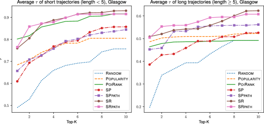
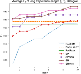
Figure 1: Average Kendall’s $\tau$ over k=1:10, for short (left) and long (middle) trajectories. (right) F₁ score on points for long trajectories. Structured recommendation methods perform best for all values of $k$. For longer trajectories, the predictions of Popularity and POIRank are permutations of the same set of POIs (that do not fully overlap with the ground truth).

Table 2 summarises the performance of all methods for top-10 recommendations. We can observe from the results that POIRank and SP, methods that convert the trajectory recommendation task into data that is amenable to off the shelf methods (ranking and structured SVM respectively) performs better than baselines but are not the best performing methods. The best results are obtained using our proposed methods SPpath, SR, and SRpath. We also compare the performance for all values of top-$k$ with $k=1,\ldots,10$, and Figure 1 shows a selection of the curves for Glasgow. We observe that our proposed methods are consistently the best for all values of $k$. See the supplement for results across all datasets on all metric variants. In particular, accounting for multiple ground truths helps – SR always performs better than SP, and similarly for the path variants of both methods. This indicates that our first extension – explicitly modelling multiple ground truths – is important to achieve good performance. We can also see that the advantages of SR, SPpath, SRpath are salient for longer trajectories, where pairwise and sequential information play a larger role.

Overall, structured recommendation methods have shown superior performance in location sequence recommendation tasks on a public benchmark. Most notably, taking into account multiple ground truths in structured prediction and modeling path constraints are important; and the effects are more pronounced in longer trajectories. Finally, we note that the unary terms in the sequence scoring function (2) can be replaced with personalised terms to each user, such as from a recommender system [8, 29]. We leave this and personalising structured recommendation as future work.

5 Conclusion

We cast the problem of sequence recommendation as a structured prediction problem. Our proposed solution extends structured SVMs to account for the new setting: first, we modified the training objective to account for the existence of multiple ground truths; second, we modified the prediction and loss augmented inference procedures to avoid predicting loops in the sequence. The inference procedures are novel applications of the list Viterbi algorithm. Experiments on real-world trajectory recommendation datasets showed that structured recommendation outperform existing, non-structured approaches. Our new viewpoint enables researchers to bring recent advances in structured prediction to bear on recommender systems problems, including further improving the efficiency of inference and learning. In the other direction techniques from recommender systems to capture latent user- and POI-representations, in sufficiently rich domains, may be used to improve the predictive power of structured prediction models.

Supplementary material to Structured Recommendation

Appendix A Model learning and prediction

In this section, we describe the 1-slack formulation for the proposed SR model and the details of the list Viterbi algorithm.

A.1 1-slack formulation for the SR model

We can use one slack variable to represent the sum of the $N$ hinge losses:

$$\xi_{i}=\max\left(0,\,\max_{\bar{\mathbf{y}}\in\mathcal{Y}}\left\{\Delta(\mathbf{y}^{(i)},\bar{\mathbf{y}})+\mathbf{w}^{\top}\Psi(\mathbf{x}^{(i)},\bar{\mathbf{y}})\right\}-\mathbf{w}^{\top}\Psi(\mathbf{x}^{(i)},\mathbf{y}^{(i)})\right).$$

Which results in the 1-slack formulation for the SR model:

A.2 The list Viterbi algorithm

We make use of the list Viterbi in four situations:

1. To avoid sequence with loops during the prediction phase of the SP and SR models

2. To make top-$k$ prediction using the SP and SR models

3. To eliminate known ground truths during the training phase (i.e. loss augmented inference) of the SR and SRpath models

4. To avoid sequence with loops during the training phase (i.e. loss augmented inference) of the SPpath and SRpath models

The serial list Viterbi algorithm [35, 32] maintains a heap (i.e. priority queue) of potential solutions, which are then checked for the desired property (for example whether there are loops). Once the requisite number of trajectories with the desired property are found, the algorithm terminates (for example once $k$ trajectories without loops are found when performing top-k prediction) The heap is initialised by running forward-backward (Algorithm 1) followed by the vanilla Viterbi (Algorithm 2).

Algorithm 1 Forward-backward procedure [43]

1:  $\forall p_{j}\in\mathcal{P},~{}\alpha_{t}(p_{j})=\begin{cases}0,~{}t=1\\ \max_{p_{i}\in\mathcal{P}}\left\{\alpha_{t-1}(p_{i})+\mathbf{w}_{ij}^{\top}\psi_{ij}(\mathbf{x},p_{i},p_{j})+\mathbf{w}_{j}^{\top}\psi_{j}(\mathbf{x},p_{j})\right\},~{}t=2,\dots,l\end{cases}$

2:  $\forall p_{i}\in\mathcal{P},~{}\beta_{t}(p_{i})=\begin{cases}0,~{}t=l\\ \max_{p_{j}\in\mathcal{P}}\left\{\mathbf{w}_{ij}^{\top}\psi_{ij}(\mathbf{x},p_{i},p_{j})+\mathbf{w}_{j}^{\top}\psi_{j}(\mathbf{x},p_{j})+\beta_{t+1}(p_{j})\right\},~{}t=l-1,\dots,1\end{cases}$

3:  $\forall p_{i},p_{j}\in\mathcal{P},~{}f_{t,t+1}(p_{i},p_{j})=\alpha_{t}(p_{i})+\mathbf{w}_{ij}^{\top}\psi_{ij}(\mathbf{x},p_{i},p_{j})+\mathbf{w}_{j}^{\top}\psi_{j}(\mathbf{x},p_{j})+\beta_{t+1}(p_{j}),~{}t=1,\dots,l-1$

Algorithm 2 Viterbi

1:  $y_{t}^{1}=\begin{cases}s,~{}t=1\\ \operatorname*{argmax}_{p\in\mathcal{P}}\left\{f_{t-1,t}(y_{t-1}^{1},p)\right\},~{}t=2,\dots,l\end{cases}$

2:  $r^{1}=\max_{p\in\mathcal{P}}\left\{\alpha_{l}(p)\right\}~{}~{}~{}\triangleright$ $r^{1}$ is the score/priority of $\mathbf{y}^{1}$

Given an existing heap containing potential trajectories, list Viterbi maintains a set of POIs $S$ to exclude, which is updated sequentially by considering the front sequence of the heap.

Recall that for trajectory recommendation we are given the query $\mathbf{x}=(s,l)$, where $s$ is the starting POI from the set of POIs $\mathcal{P}$, and $l$ is the desired length of the trajectory. We assume the score function is of the form $\mathbf{w}^{\top}\Psi$ where $\Psi$ is the joint feature vector. $\mathbf{w}$ could be the value of the weight in the current iteration in training, or the learned weight vector during prediction.

The list Viterbi algorithm for performing top-$k$ prediction is described in Algorithm 3. To eliminating known ground truths in loss augmented inference, we modify the forward-backward procedure (Algorithm 1) to account for the loss term $\Delta(\cdot,\cdot)$, and Algorithm 2 and Algorithm 3 can be used without modification.

Algorithm 3 The list Viterbi algorithm for top-$K$ prediction [35, 32]

1:  Input: $\mathbf{x}=(s,l),~{}\mathcal{P},~{}\mathbf{w},~{}\Psi,~{}K$

2:  Initialise score matrices $\alpha,~{}\beta,~{}f_{t,t+1}$, a max-heap $H$, result set $R$, $k=0$.

3:  $\triangleright$ Do the forward-backward procedure (Algorithm 1)

4:  $\triangleright$ Identify the best (scored) trajectory $\mathbf{y}^{1}=(y_{1}^{1},\dots,y_{l}^{1})$ with Viterbi (Algorithm 2). This may be a trajectory that violates the desired condition.

5:  $H.\textit{push}\left(r^{1},~{}(\mathbf{y}^{1},\textsc{nil},\emptyset)\right)$

6:  Set $R=\emptyset$, the list of trajectories to be returned.

7:  while $H\neq\emptyset$ and $k<\,|\mathcal{P}|^{l-1}-\prod_{t=2}^{l}(|\mathcal{P}|-t+1)+K$ do

8:     $r^{k},~{}(\mathbf{y}^{k},I,S)=H.\textit{pop}()~{}~{}~{}\triangleright$ $r^{k}$ is the score of $\mathbf{y}^{k}=(y_{1}^{k},\dots,y_{l}^{k})$, $I$ is the partition index, and $S$ is the exclude set

9:     $k=k+1$

10:     Add $\mathbf{y}^{k}$ to $R$ if it satisfies the desired property

11:     return  $R$ if it contains the required number of trajectories

12:     $I^{\prime}=\begin{cases}2,&I=\textsc{nil}\\ I,&\text{otherwise}\end{cases}$

13:     for $t=I^{\prime},\dots,l$ do

14:        $S^{\prime}=\begin{cases}S\cup\{y_{t}^{k}\},&t=I^{\prime}\\ \{y_{t}^{k}\},&\text{otherwise}\end{cases}$

15:        $y^{\prime}_{j}=\begin{cases}y_{j}^{k},&j=1,\dots,t-1\\ \operatorname*{argmax}_{p\in\mathcal{P}\setminus S^{\prime}}\left\{f_{t-1,t}(y_{t-1}^{k},p)\right\},&j=t\\ \operatorname*{argmax}_{p\in\mathcal{P}}\left\{f_{j-1,j}(y^{\prime}_{j-1},p)\right\},&j=t+1,\dots,l\end{cases}$

16:        $r^{\prime}=r^{k}+f_{t-1,t}(y_{t-1}^{k},y^{\prime}_{t})-f_{t-1,t}(y_{t-1}^{k},y_{t}^{k})$

17:        $H.\textit{push}(r^{\prime},(\mathbf{y}^{\prime},t,S^{\prime}))$

18:     end for

19:  end while

Appendix B Experiment

In this section, we describe trajectory dataset used in experiments as well as features for each methods. In addition, the details of evaluation and empirical results are also described.

B.1 Photo trajectory dataset and features

Dataset. In the interests of reproducibility we present further details of our empirical experiment. The histogram of the number of trajectories per query is shown in Figure 2, where we can see each query has 4-9 ground truths (i.e. trajectories) on average, and 30-60 trajectories at most. The histogram of trajectory length (i.e. the number of POIs in a trajectory) is shown in Figure 3, where we can see the majority are short trajectories (i.e. length $\leq$ 5).

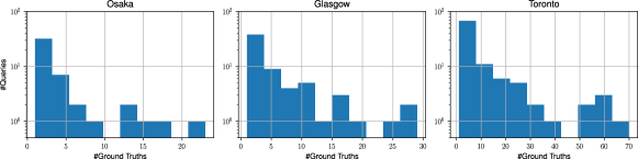
Figure 2: Histograms of the number of trajectories per query.

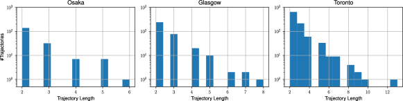
Figure 3: Histograms of trajectory length.

Features. The POI-query features used by PoiRank, SP and SR methods and their extensions (i.e. the SPpath and SRpath models) are shown in Table 3, pairwise features used in SP and SR methods and their extensions are shown in Table 4.

Table 3: POI-query features: features of POI $p$ with respect to query $(s,l)$

Feature	Description
category	one-hot encoding of the category of $p$
neighbourhood	one-hot encoding of the POI cluster that $p$ resides in
popularity	logarithm of POI popularity of $p$
nVisit	logarithm of the total number of visit by all users at $p$
avgDuration	logarithm of the average visit duration at $p$
trajLen	trajectory length $l$, i.e., the number of POIs required
sameCatStart	$1$ if the category of $p$ is the same as that of $s$, $-1$ otherwise
sameNeighbourhoodStart	$1$ if $p$ resides in the same POI cluster as $s$, $-1$ otherwise
diffPopStart	real-valued difference in POI popularity of $p$ from that of $s$
diffNVisitStart	real-valued difference in the total number of visit at $p$ from that at $s$
diffDurationStart	real-valued difference in average duration at $p$ from that at $s$
distStart	distance between $p$ and $s$, calculated using the Haversine formula

Table 4: Pairwise POI features

Feature	Description
category	category of POI
neighbourhood	the cluster that a POI resides in
popularity	(discretised) popularity of POI
nVisit	(discretised) total number of visit at POI
avgDuration	(discretised) average duration at POI

B.2 Evaluation settings

Top-k prediction for baselines.

• To perform top-$k$ prediction with Random baseline, we simply repeat the Random method $k$ times.

• To perform top-$k$ prediction with Popularity and PoiRank, we make use of the list Viterbi algorithm (Algorithm 3 to get $k$ best scored paths, in particular, for Popularity, the score of a path is the accumulated popularity of all POIs in the path; for PoiRank, the score of a path is the likelihood (the ranking scores for POIs are first transformed into a probability distribution using the softmax function, as described in [12]).

To evaluate the performance of a certain recommendation algorithm, we need to measure the similarity (or loss) given prediction $\hat{\mathbf{y}}$ and ground truth $\mathbf{y}$.

F₁ score on points. F₁ score on points [11] cares about only the set of correctly recommended POIs.

$$F_{1}(\mathbf{y},\hat{\mathbf{y}})=\frac{2P_{\textsc{point}}R_{\textsc{point}}}{P_{\textsc{point}}+R_{\textsc{point}}}$$

where $P_{\textsc{point}}$, $R_{\textsc{point}}$ are respectively the precision and recall for points in $\hat{\mathbf{y}}$ and $\mathbf{y}$. If $|\hat{\mathbf{y}}|=|\mathbf{y}|$, this metric is just the unordered Hamming loss, i.e., Hamming loss between two binary indicator vectors of size $|\mathcal{P}|$.

F₁ score on pairs. To take into account the orders in recommended sequence, we also use the F₁ score on pairs [12] measure, which considers the set of correctly predicted POI pairs,

$$\text{pairs-F}_{1}(\mathbf{y},\hat{\mathbf{y}})=\frac{2P_{\textsc{pair}}R_{\textsc{pair}}}{P_{\textsc{pair}}+R_{\textsc{pair}}}$$

where $P_{\textsc{point}}$, $R_{\textsc{point}}$ are respectively the precision and recall for all possible pairs of $\hat{\mathbf{y}}$ and $\mathbf{y}$.

Kendall’s $\tau$ with ties Alternatively, we can cast a trajectory $\mathbf{y}=y_{1:l}$ as a ranking of POIs in $\mathcal{P}$, where $y_{j}$ has a rank $|\mathcal{P}|-j+1$ and any other POI $p\notin\mathbf{y}$ has a rank $0$ ($0$ is an arbitrary choice), then we can make use of ranking evaluation metrics such as Kendall’s $\tau$ by taking care of ties in ranks. In particular, given a prediction $\hat{\mathbf{y}}=\hat{y_{1:l}}$ and ground truth $\mathbf{y}=y_{1:l}$, we produce two ranks for $\mathbf{y}$ and $\hat{\mathbf{y}}$ with respect to a specific ordering of POIs $(p_{1},p_{2},\dots,p_{|\mathcal{P}|})$:

$$r_{i} =\sum_{j=1}^{l}(|\mathcal{P}|-j+1)\llbracket p_{i}=y_{j}\rrbracket,~{}i=1,\dots,|\mathcal{P}|$$

$$\hat{r}_{i} =\sum_{j=1}^{l}(|\mathcal{P}|-j+1)\llbracket p_{i}=\hat{y}_{j}\rrbracket,~{}i=1,\dots,|\mathcal{P}|$$

where POIs not in $\mathbf{y}$ will have a rank of $0$. Then we compute the following metrics:

• the number of concordant pairs $C=\frac{1}{2}\sum_{i,j}\left(\llbracket r_{i}<r_{j}\rrbracket\llbracket\hat{r}_{i}<\hat{r}_{j}\rrbracket+\llbracket r_{i}>r_{j}\rrbracket\llbracket\hat{r}_{i}>\hat{r}_{j}\rrbracket\right)$

• the number of discordant pairs $D=\frac{1}{2}\sum_{i,j}\left(\llbracket r_{i}<r_{j}\rrbracket\llbracket\hat{r}_{i}>\hat{r}_{j}\rrbracket+\llbracket r_{i}>r_{j}\rrbracket\llbracket\hat{r}_{i}<\hat{r}_{j}\rrbracket\right)$

• the number of ties in ground truth $\mathbf{y}$: $T_{\mathbf{y}}=\frac{1}{2}\sum_{i\neq j}\llbracket r_{i}=r_{j}\rrbracket=\frac{1}{2}\left(|\mathcal{P}|-l\right)\left(|\mathcal{P}|-l-1\right)$

• the number of ties in prediction $\hat{\mathbf{y}}$: $T_{\hat{\mathbf{y}}}=\frac{1}{2}\sum_{i\neq j}\llbracket\hat{r}_{i}=\hat{r}_{j}\rrbracket=\frac{1}{2}\left(|\mathcal{P}|-l\right)\left(|\mathcal{P}|-l-1\right)$

• the number of ties in both $\mathbf{y}$ and $\hat{\mathbf{y}}$: $T_{\mathbf{y},\hat{\mathbf{y}}}=\frac{1}{2}\sum_{i\neq j}\llbracket r_{i}=r_{j}\rrbracket\llbracket\hat{r}_{i}=\hat{r}_{j}\rrbracket$

Kendall’s $\tau$ (version $b$) [44, 41] is

$$\tau_{b}(\mathbf{y},\hat{\mathbf{y}})=\frac{C-D}{\sqrt{(C+D+T)(C+D+U)}},$$

where $T=T_{\mathbf{y}}-T_{\mathbf{y},\hat{\mathbf{y}}}$ and $U=T_{\hat{\mathbf{y}}}-T_{\mathbf{y},\hat{\mathbf{y}}}$.

B.3 Empirical results

The effects of $k$ for top-$k$ prediction. The performance of baselines and structured recommendation algorithms for top-$k$ ($k=1,3,5,10$) prediction are shown in the following tables. Bold entries: best performing method for each metric; italicised entries: the next best.

Table 5: Results on trajectory recommendation datasets on best of top-1.

	Kendall’s $\tau$
	Random	Popularity	PoiRank	SP	SPpath	SR	SRpath
Glasgow	$0.430\pm 0.031$	$0.644\pm 0.036$	$\mathbf{0.733\pm 0.030}$	$0.564\pm 0.029$	$0.615\pm 0.034$	$0.708\pm 0.031$	$\mathit{0.712\pm 0.031}$
Osaka	$0.420\pm 0.030$	$0.566\pm 0.034$	$\mathbf{0.644\pm 0.040}$	$0.525\pm 0.037$	$0.525\pm 0.039$	$0.608\pm 0.042$	$\mathit{0.613\pm 0.044}$
Toronto	$0.394\pm 0.025$	$0.626\pm 0.023$	$\mathit{0.714\pm 0.024}$	$0.543\pm 0.026$	$0.572\pm 0.026$	$0.714\pm 0.026$	$\mathbf{0.717\pm 0.026}$
	F1 score on points
Glasgow	$0.478\pm 0.027$	$0.681\pm 0.032$	$\mathbf{0.764\pm 0.027}$	$0.604\pm 0.026$	$0.653\pm 0.031$	$0.741\pm 0.028$	$\mathit{0.743\pm 0.028}$
Osaka	$0.459\pm 0.027$	$0.601\pm 0.031$	$\mathbf{0.678\pm 0.037}$	$0.555\pm 0.034$	$0.558\pm 0.036$	$0.638\pm 0.039$	$\mathit{0.645\pm 0.040}$
Toronto	$0.461\pm 0.020$	$0.671\pm 0.021$	$\mathit{0.756\pm 0.021}$	$0.594\pm 0.023$	$0.623\pm 0.023$	$0.753\pm 0.023$	$\mathbf{0.757\pm 0.022}$
	F1 score on pairs
Glasgow	$0.154\pm 0.035$	$0.426\pm 0.051$	$\mathbf{0.545\pm 0.046}$	$0.289\pm 0.042$	$0.389\pm 0.048$	$0.506\pm 0.048$	$\mathit{0.516\pm 0.048}$
Osaka	$0.104\pm 0.037$	$0.281\pm 0.051$	$\mathbf{0.428\pm 0.059}$	$0.243\pm 0.052$	$0.254\pm 0.055$	$0.375\pm 0.059$	$\mathit{0.401\pm 0.060}$
Toronto	$0.143\pm 0.025$	$0.384\pm 0.034$	$0.506\pm 0.036$	$0.299\pm 0.033$	$0.340\pm 0.035$	$\mathit{0.530\pm 0.037}$	$\mathbf{0.533\pm 0.037}$

Table 6: Results on trajectory recommendation datasets on best of top-3.

	Kendall’s $\tau$
	Random	Popularity	PoiRank	SP	SPpath	SR	SRpath
Glasgow	$0.563\pm 0.031$	$0.693\pm 0.036$	$0.781\pm 0.030$	$0.666\pm 0.033$	$0.688\pm 0.032$	$\mathit{0.803\pm 0.029}$	$\mathbf{0.808\pm 0.030}$
Osaka	$0.556\pm 0.037$	$0.666\pm 0.039$	$\mathbf{0.726\pm 0.042}$	$0.630\pm 0.044$	$0.698\pm 0.040$	$\mathit{0.711\pm 0.042}$	$0.697\pm 0.042$
Toronto	$0.521\pm 0.026$	$0.670\pm 0.025$	$0.746\pm 0.023$	$0.629\pm 0.027$	$0.650\pm 0.027$	$\mathbf{0.753\pm 0.025}$	$\mathit{0.749\pm 0.024}$
	F1 score on points
Glasgow	$0.598\pm 0.028$	$0.722\pm 0.033$	$0.803\pm 0.027$	$0.698\pm 0.030$	$0.716\pm 0.029$	$\mathit{0.825\pm 0.026}$	$\mathbf{0.829\pm 0.026}$
Osaka	$0.587\pm 0.034$	$0.691\pm 0.035$	$\mathbf{0.750\pm 0.039}$	$0.656\pm 0.040$	$0.724\pm 0.037$	$\mathit{0.735\pm 0.038}$	$0.723\pm 0.039$
Toronto	$0.577\pm 0.022$	$0.704\pm 0.023$	$0.776\pm 0.021$	$0.674\pm 0.023$	$0.693\pm 0.023$	$\mathbf{0.784\pm 0.022}$	$\mathit{0.780\pm 0.021}$
	F1 score on pairs
Glasgow	$0.300\pm 0.043$	$0.524\pm 0.053$	$0.625\pm 0.046$	$0.464\pm 0.049$	$0.481\pm 0.048$	$\mathit{0.666\pm 0.045}$	$\mathbf{0.678\pm 0.045}$
Osaka	$0.288\pm 0.055$	$0.448\pm 0.058$	$\mathbf{0.578\pm 0.060}$	$0.425\pm 0.062$	$0.511\pm 0.059$	$\mathit{0.549\pm 0.060}$	$0.520\pm 0.059$
Toronto	$0.281\pm 0.032$	$0.477\pm 0.036$	$0.575\pm 0.035$	$0.429\pm 0.037$	$0.461\pm 0.037$	$\mathbf{0.592\pm 0.036}$	$\mathit{0.584\pm 0.036}$

Table 7: Results on trajectory recommendation datasets on best of top-5.

	Kendall’s $\tau$
	Random	Popularity	PoiRank	SP	SPpath	SR	SRpath
Glasgow	$0.623\pm 0.029$	$0.727\pm 0.037$	$0.801\pm 0.030$	$0.727\pm 0.033$	$0.743\pm 0.031$	$\mathit{0.826\pm 0.028}$	$\mathbf{0.832\pm 0.028}$
Osaka	$0.618\pm 0.038$	$0.674\pm 0.038$	$\mathbf{0.750\pm 0.040}$	$0.678\pm 0.045$	$0.735\pm 0.039$	$\mathit{0.741\pm 0.039}$	$0.729\pm 0.041$
Toronto	$0.574\pm 0.025$	$0.687\pm 0.025$	$0.754\pm 0.023$	$0.662\pm 0.027$	$0.683\pm 0.026$	$\mathbf{0.778\pm 0.023}$	$\mathit{0.769\pm 0.024}$
	F1 score on points
Glasgow	$0.655\pm 0.026$	$0.754\pm 0.033$	$0.821\pm 0.026$	$0.755\pm 0.030$	$0.770\pm 0.027$	$\mathit{0.847\pm 0.024}$	$\mathbf{0.850\pm 0.025}$
Osaka	$0.646\pm 0.035$	$0.699\pm 0.034$	$\mathbf{0.772\pm 0.037}$	$0.700\pm 0.041$	$0.757\pm 0.036$	$\mathit{0.761\pm 0.036}$	$0.751\pm 0.037$
Toronto	$0.624\pm 0.022$	$0.719\pm 0.023$	$0.781\pm 0.021$	$0.705\pm 0.023$	$0.724\pm 0.022$	$\mathbf{0.808\pm 0.021}$	$\mathit{0.798\pm 0.021}$
	F1 score on pairs
Glasgow	$0.377\pm 0.044$	$0.590\pm 0.052$	$0.670\pm 0.045$	$0.563\pm 0.048$	$0.573\pm 0.047$	$\mathit{0.701\pm 0.043}$	$\mathbf{0.715\pm 0.044}$
Osaka	$0.375\pm 0.058$	$0.459\pm 0.057$	$\mathbf{0.607\pm 0.058}$	$0.507\pm 0.064$	$0.568\pm 0.058$	$\mathit{0.584\pm 0.058}$	$0.575\pm 0.058$
Toronto	$0.343\pm 0.034$	$0.504\pm 0.036$	$0.593\pm 0.034$	$0.483\pm 0.037$	$0.510\pm 0.037$	$\mathbf{0.624\pm 0.035}$	$\mathit{0.610\pm 0.035}$

Table 8: Results on trajectory recommendation datasets on best of top-10.

	Kendall’s $\tau$
	Random	Popularity	PoiRank	SP	SPpath	SR	SRpath
Glasgow	$0.703\pm 0.029$	$0.748\pm 0.036$	$0.830\pm 0.029$	$0.790\pm 0.030$	$0.787\pm 0.029$	$\mathbf{0.868\pm 0.026}$	$\mathit{0.853\pm 0.026}$
Osaka	$0.685\pm 0.035$	$0.768\pm 0.038$	$0.787\pm 0.037$	$0.749\pm 0.043$	$\mathit{0.791\pm 0.036}$	$0.777\pm 0.036$	$\mathbf{0.803\pm 0.034}$
Toronto	$0.652\pm 0.024$	$0.719\pm 0.024$	$0.784\pm 0.023$	$0.697\pm 0.027$	$0.719\pm 0.026$	$\mathbf{0.802\pm 0.022}$	$\mathit{0.797\pm 0.022}$
	F1 score on points
Glasgow	$0.731\pm 0.026$	$0.771\pm 0.033$	$0.847\pm 0.025$	$0.810\pm 0.027$	$0.807\pm 0.026$	$\mathbf{0.883\pm 0.023}$	$\mathit{0.868\pm 0.023}$
Osaka	$0.703\pm 0.032$	$0.786\pm 0.034$	$0.804\pm 0.034$	$0.770\pm 0.039$	$\mathit{0.809\pm 0.033}$	$0.793\pm 0.033$	$\mathbf{0.820\pm 0.031}$
Toronto	$0.696\pm 0.021$	$0.746\pm 0.022$	$0.807\pm 0.020$	$0.733\pm 0.023$	$0.755\pm 0.022$	$\mathbf{0.828\pm 0.019}$	$\mathit{0.823\pm 0.020}$
	F1 score on pairs
Glasgow	$0.495\pm 0.046$	$0.623\pm 0.051$	$0.726\pm 0.043$	$0.658\pm 0.046$	$0.648\pm 0.045$	$\mathbf{0.770\pm 0.039}$	$\mathit{0.746\pm 0.041}$
Osaka	$0.451\pm 0.057$	$0.626\pm 0.055$	$0.661\pm 0.056$	$0.620\pm 0.061$	$\mathit{0.664\pm 0.055}$	$0.637\pm 0.055$	$\mathbf{0.671\pm 0.053}$
Toronto	$0.438\pm 0.034$	$0.550\pm 0.035$	$0.649\pm 0.033$	$0.530\pm 0.037$	$0.552\pm 0.036$	$\mathbf{0.660\pm 0.033}$	$\mathit{0.657\pm 0.034}$

Performance on short and long trajectories. The performance of baselines and structured recommendation algorithms for short (length $<$ 5) and long (length $\geq$ 5) trajectories with top-$k$ ($k=1:10$) prediction are shown in the following figures.

See pages 1- of plot_topk.pdf

References

- [1] D. Goldberg, D. Nichols, B. M. Oki, and D. Terry, “Using collaborative filtering to weave an information tapestry,” Commun. ACM, vol. 35, Dec. 1992.
- [2] B. Sarwar, G. Karypis, J. Konstan, and J. Riedl, “Item-based collaborative filtering recommendation algorithms,” in WWW ’01, (New York, NY, USA), pp. 285–295, ACM, 2001.
- [3] Y. Koren, “Factor in the neighbors: Scalable and accurate collaborative filtering,” ACM Trans. Knowl. Discov. Data, vol. 4, pp. 1:1—-1:24, Jan. 2010.
- [4] G. Linden, B. Smith, and J. York, “Amazon.com Recommendations: Item-to-Item Collaborative Filtering,” IEEE Internet Computing, vol. 7, pp. 76–80, Jan. 2003.
- [5] D. Agarwal, B.-C. Chen, P. Elango, and R. Ramakrishnan, “Content recommendation on web portals,” Commun. ACM, vol. 56, pp. 92–101, June 2013.
- [6] X. Amatriain and J. Basilico, Recommender Systems in Industry: A Netflix Case Study, pp. 385–419. Boston, MA: Springer US, 2015.
- [7] C. A. Gomez-Uribe and N. Hunt, “The Netflix recommender system: Algorithms, business value, and innovation,” ACM Transactions on Management Information Systems, vol. 6, pp. 13:1–13:19, Dec. 2015.
- [8] Y. Koren, R. Bell, and C. Volinsky, “Matrix factorization techniques for recommender systems,” Computer, vol. 42, pp. 30–37, Aug. 2009.
- [9] X. Lu, C. Wang, J.-M. Yang, Y. Pang, and L. Zhang, “Photo2Trip: Generating travel routes from geo-tagged photos for trip planning,” MM ’10, pp. 143–152, ACM, 2010.
- [10] E. H.-C. Lu, C.-Y. Chen, and V. S. Tseng, “Personalized trip recommendation with multiple constraints by mining user check-in behaviors,” SIGSPATIAL ’12, pp. 209–218, ACM, 2012.
- [11] K. H. Lim, J. Chan, C. Leckie, and S. Karunasekera, “Personalized tour recommendation based on user interests and points of interest visit durations,” in Proceedings of the 24th International Joint Conference on Artificial Intelligence, pp. 1778–1784, 2015.
- [12] D. Chen, C. S. Ong, and L. Xie, “Learning points and routes to recommend trajectories,” in Proceedings of the 25th ACM International Conference on Information and Knowledge Management, pp. 2227–2232, 2016.
- [13] B. McFee and G. Lanckriet, “The natural language of playlists,” in 12th International Symposium for Music Information Retrieval (ISMIR2011)), October 2011.
- [14] S. Chen, J. L. Moore, D. Turnbull, and T. Joachims, “Playlist prediction via metric embedding,” in Proceedings of the 18th ACM SIGKDD international conference on Knowledge discovery and data mining, pp. 714–722, ACM, 2012.
- [15] B. Hidasi, A. Karatzoglou, L. Baltrunas, and D. Tikk, “Session-based recommendations with recurrent neural networks,” arXiv preprint arXiv:1511.06939, 2015.
- [16] K. Choi, G. Fazekas, and M. Sandler, “Towards playlist generation algorithms using RNNs trained on within-track transitions,” arXiv preprint arXiv:1606.02096, 2016.
- [17] L. Dehaspe, H. Toivonen, and R. D. King, “Finding frequent substructures in chemical compounds.,” in KDD, vol. 98, p. 1998, 1998.
- [18] A. Antikacioglu, R. Ravi, and S. Sridhar, “Recommendation subgraphs for web discovery,” in Proceedings of the 24th International Conference on World Wide Web, pp. 77–87, ACM, 2015.
- [19] I. Tsochantaridis, T. Joachims, T. Hofmann, and Y. Altun, “Large margin methods for structured and interdependent output variables,” Journal of Machine Learning Research, vol. 6, no. Sep, pp. 1453–1484, 2005.
- [20] T. Joachims, T. Hofmann, Y. Yue, and C.-N. Yu, “Predicting structured objects with support vector machines,” Communications of the ACM, vol. 52, no. 11, pp. 97–104, 2009.
- [21] D. B. West et al., Introduction to graph theory, vol. 2. Prentice hall Upper Saddle River, 2001.
- [22] Netflix, “Netflix Prize.” http://www.netflixprize.com/, 2006.
- [23] J. Bao, Y. Zheng, D. Wilkie, and M. Mokbel, “Recommendations in location-based social networks: a survey,” GeoInformatica, vol. 19, no. 3, pp. 525–565, 2015.
- [24] Y. Zheng, “Trajectory data mining: an overview,” ACM Transactions on Intelligent Systems and Technology, vol. 6, no. 3, p. 29, 2015.
- [25] Y. Zheng, L. Capra, O. Wolfson, and H. Yang, “Urban computing: concepts, methodologies, and applications,” ACM Transactions on Intelligent Systems and Technology, vol. 5, no. 3, p. 38, 2014.
- [26] S. Rendle, C. Freudenthaler, and L. Schmidt-Thieme, “Factorizing personalized markov chains for next-basket recommendation,” in WWW ’10, (New York, NY, USA), pp. 811–820, ACM, 2010.
- [27] P. Wang, J. Guo, Y. Lan, J. Xu, S. Wan, and X. Cheng, “Learning hierarchical representation model for nextbasket recommendation,” in SIGIR ’15, (New York, NY, USA), pp. 403–412, ACM, 2015.
- [28] F. Yu, Q. Liu, S. Wu, L. Wang, and T. Tan, “A dynamic recurrent model for next basket recommendation,” in Proceedings of the 39th International ACM SIGIR conference on Research and Development in Information Retrieval, pp. 729–732, ACM, 2016.
- [29] S. Rendle, C. Freudenthaler, Z. Gantner, and L. Schmidt-Thieme, “BPR: Bayesian personalized ranking from implicit feedback,” UAI ’09, pp. 452–461, AUAI Press, 2009.
- [30] N. Ratliff, J. A. Bagnell, and M. Zinkevich, “Subgradient methods for maximum margin structured learning,” in ICML workshop on learning in structured output spaces, vol. 46, Citeseer, 2006.
- [31] S. Lacoste-julien, M. Jaggi, M. Schmidt, and P. Pletscher, “Block-coordinate Frank-Wolfe optimization for structural SVMs,” in Proceedings of the 30th International Conference on Machine Learning (ICML’13), pp. 53–61, 2013.
- [32] N. Seshadri and C.-E. Sundberg, “List Viterbi decoding algorithms with applications,” IEEE Transactions on Communications, vol. 42, no. 234, pp. 313–323, 1994.
- [33] C. Nill and C.-E. Sundberg, “List and soft symbol output viterbi algorithms: Extensions and comparisons,” IEEE Transactions on Communications, vol. 43, no. 234, pp. 277–287, 1995.
- [34] F. K. Soong and E.-F. Huang, “A tree-trellis based fast search for finding the n-best sentence hypotheses in continuous speech recognition,” in Acoustics, Speech, and Signal Processing, 1991. ICASSP-91., 1991 International Conference on, pp. 705–708, IEEE, 1991.
- [35] D. Nilsson and J. Goldberger, “Sequentially finding the N-best list in hidden Markov models,” in Proceedings of the 17th international joint conference on Artificial intelligence, pp. 1280–1285, Morgan Kaufmann Publishers Inc., 2001.
- [36] D. L. Applegate, R. E. Bixby, V. Chvatal, and W. J. Cook, The traveling salesman problem: a computational study. Princeton university press, 2011.
- [37] D. Lian, C. Zhao, X. Xie, G. Sun, E. Chen, and Y. Rui, “GeoMF: Joint geographical modeling and matrix factorization for point-of-interest recommendation,” KDD ’14, pp. 831–840, ACM, 2014.
- [38] N. Christofides, “Worst-case analysis of a new heuristic for the travelling salesman problem,” Tech. Rep. 388, Graduate School of Industrial Administration, CMU, 1976.
- [39] B. Thomee, B. Elizalde, D. A. Shamma, K. Ni, G. Friedland, D. Poland, D. Borth, and L.-J. Li, “YFCC100M: The new data in multimedia research,” Communications of the ACM, vol. 59, no. 2, pp. 64–73, 2016.
- [40] P. Burman, “A comparative study of ordinary cross-validation, v-fold cross-validation and the repeated learning-testing methods,” Biometrika, vol. 76, no. 3, pp. 503–514, 1989.
- [41] A. Agresti, Analysis of ordinal categorical data, vol. 656. John Wiley & Sons, 2010.
- [42] O. Russakovsky, J. Deng, H. Su, J. Krause, S. Satheesh, S. Ma, Z. Huang, A. Karpathy, A. Khosla, M. Bernstein, et al., “ImageNet large scale visual recognition challenge,” International Journal of Computer Vision, vol. 115, no. 3, pp. 211–252, 2015.
- [43] L. R. Rabiner, “A tutorial on hidden Markov models and selected applications in speech recognition,” Proceedings of the IEEE, vol. 77, no. 2, pp. 257–286, 1989.
- [44] M. G. Kendall, “The treatment of ties in ranking problems,” Biometrika, vol. 33, no. 3, pp. 239–251, 1945.