Investigating cluster astrophysics and cosmology with cross-correlation of the thermal Sunyaev–Zel’dovich effect and weak lensing

Abstract

Recent detections of the cross-correlation of the thermal Sunyaev–Zel’dovich (tSZ) effect and weak gravitational lensing (WL) enable unique studies of cluster astrophysics and cosmology. In this work, we present constraints on the amplitude of the non-thermal pressure fraction in galaxy clusters, $\alpha_{0}$, and the amplitude of the matter power spectrum, $\sigma_{8}$, using measurements of the tSZ power spectrum from Planck, and the tSZ-WL cross-correlation from Planck and the Red Cluster Sequence Lensing Survey. We fit the data to a semi-analytic model with the covariance matrix using $N$-body simulations. We find that the tSZ power spectrum alone prefers $\sigma_{8}\sim 0.85$ and a large fraction of non-thermal pressure ($\alpha_{0}\sim 0.2$–$0.3$). The tSZ-WL cross-correlation on the other hand prefers a significantly lower $\sigma_{8}\sim 0.6$, and low $\alpha_{0}\sim 0.05$. We show that this tension can be mitigated by allowing for a steep slope in the stellar-mass-halo-mass relation, which would cause a reduction of the gas in low-mass halos. In such a model, the combined data prefer $\sigma_{8}\sim 0.7$ and $\alpha_{0}\sim 0.2$, consistent with predictions from hydrodynamical simulations.

1 Introduction

The observation of the anisotropy of cosmic microwave background (CMB) provides us with generous information of our Universe. The Sunyaev–Zel’dovich (SZ) effect (Sunyaev & Zeldovich, 1972, 1980) is one of the effects which give rise to the anisotropy after CMB photons decouple with the hot plasma. As CMB photons are scattered by hot electrons, energy transfer occurs via Compton scattering. As a result, the energy spectrum of CMB deviates from the black-body spectrum. There are two types of SZ effects, one is thermal SZ effect (tSZ), which is due to the thermal motion of hot gas, and the other one is kinetic SZ effect (kSZ), which is due to the bulk motion of gas. Since the hot electrons sourcing the tSZ signal originate predominantly from massive halos, the tSZ signal reflects thermodynamic properties of intracluster medium (ICM). Though SZ effects have been important probes into the structure formation in the Universe and astrophysics of the ICM, the measurement of SZ effects is challenging because of the small amplitude of the signal and foreground contamination. Due to significant improvement in resolution and sensitivity, several CMB experiments have been able to detect the tSZ effect (see, e.g., Hasselfield et al., 2013; Bleem et al., 2015; Planck Collaboration, 2016b). In order to make full use of the recent observations, the accurate and precise modeling of SZ effects is essential for cosmology.

There are various methods for modeling the tSZ effect. One of the methods is the analytical modeling of radial profiles of gas density and pressure (Komatsu & Seljak, 2001, 2002; Ostriker et al., 2005). Then, one can obtain the tSZ power spectrum using the halo model (Cole & Kaiser, 1988; Komatsu & Kitayama, 1999). However, the evolution of gas is governed by complex baryonic physics, e.g., star formation, feedback, and radiative cooling, which are difficult to model analytically. This difficulty directly leads to the uncertainty of the model. One of the solutions to take baryonic physics into account properly is employing hydrodynamical simulations. The gas pressure profile of halos with different masses and redshifts can be measured from cosmological hydrodynamical simulations which include baryonic physics and the obtained profile is applied to model the tSZ signal based on a halo model (Battaglia et al., 2010, 2012). Alternatively, one can also obtain the gas pressure field in the Universe from hydrodynamical simulation, and hence the tSZ signal directly by integrating the pressure field in the line-of-sight direction (see, e.g., McCarthy et al., 2014; Dolag et al., 2016).

However, running hydrodynamical simulations is computationally expensive, and the volume covered by the simulation is limited. To overcome these problems, a realistic solution is the semi-analytic prescription which combines analytical modeling and $N$-body simulations. In Sehgal et al. (2010); Trac et al. (2011), the authors run $N$-body simulations and create halo catalogs from the simulations. From the halo mass, the gas pressure profile of the halo is obtained analytically, and then gas pressure is pasted onto each particle in the $N$-body simulation. Dark matter only simulations are computationally more efficient, and can therefore be used to cover larger volumes than hydrodynamical simulations.

Furthermore, in this method we can incorporate various factors which are not taken into account in the analytical models, e.g., asphericity of halos or the effects of substructures. Another way to model the pressure profile is to make use of X-ray or tSZ observations (Arnaud et al., 2010; Planck Collaboration, 2013). Since the pressure profile can be inferred from these observations, we can learn about the relation between pressure and cluster mass and redshift. Though such observations are typically limited at the low redshift, substantial fraction of the tSZ power spectrum comes from the high redshift clusters. This fact leads to the uncertainty in the modeling.

In addition to tSZ, we focus on weak gravitational lensing (WL) by the large-scale structure, so-called comic shear (for a review, see Bartelmann & Schneider, 2001; Munshi et al., 2008; Kilbinger, 2015). The path of photons from distant galaxies is distorted by gravitational potential of intervening matter. WL reflects the abundance of matter in the line-of-sight direction and thus can be a promising probe into the nature of dark matter and dark energy. Unlike the tSZ, WL is mostly determined by gravity and less affected by baryonic physics. The nonlinear evolution by gravity is well modeled by $N$-body simulations.

The information that can be extracted either from WL or tSZ is limited; WL suffers from degeneracies between cosmological parameters, while tSZ suffers from astrophysical uncertainties. Thus, a combination of WL and tSZ can arguably be more efficient in extracting cosmological parameters. For this purpose, we focus on cross-correlation of WL and tSZ in addition to the auto-power spectrum of the tSZ. The cross-correlation analysis has a possibility to enable us to place more stringent constraints on cosmological parameters evading the astrophysical uncertainties and implications to physics of ICM (Munshi et al., 2014; Ma et al., 2015; Hojjati et al., 2015; Battaglia et al., 2015). Furthermore, the cross-correlation has already been detected by several groups (van Waerbeke et al., 2014; Hill & Spergel, 2014; Hojjati et al., 2017, note that their Compton-$y$ maps are based on Planck data but constructed in different ways.) and is one of scientific goals of current and forthcoming surveys, e.g. the Hyper Suprime-Cam survey (HSC; Aihara et al., 2017) , Dark Energy Survey (DES; Dark Energy Survey Collaboration, 2016) , and Large Synoptic Survey Telescope (LSST; LSST Science Collaboration, 2009) for WL, and Atacama Cosmology Telescope (ACT/ACTPol; Niemack et al., 2010; Swetz et al., 2011) and South Pole Telescope (SPT/SPTPol; Carlstrom et al., 2011; Austermann et al., 2012) for tSZ.

It is timely to investigate the ability of the cross-correlation with numerical simulations. In this paper, we combine the output from an $N$-body simulation with a semi-analytic model for the pressure, in order to create mock tSZ and WL maps. Using these maps, we estimate the covariance matrix of the tSZ power spectrum and the tSZ-WL cross-correlation. The main results of this analysis are the constrains on $\sigma_{8}$ and the amount of non-thermal pressure in the ICM, derived from recent measurements from Planck (Planck Collaboration, 2016b) and the Red Cluster Sequence Lensing Survey (RCSLenS) (Hildebrandt et al., 2016; Hojjati et al., 2017). Recently, it is reported that there is a tension of inferred $\sigma_{8}$ between the measurements of CMB temperature anisotropy and large scale structure, e.g., power spectrum of WL (Battye et al., 2015; Leauthaud et al., 2017). Furthermore, tSZ power spectra measured from SPT and ACT are lower than the prediction based on Planck best-fit cosmological parameters (Planck Collaboration, 2016b). This fact also may be related to the $\sigma_{8}$ tension, though there is a possibility that the incomplete separation of foreground contamination causes the low amplitude of the power spectrum. The tSZ-WL cross-correlation along with tSZ power spectrum is one of promissing probes into this problem.

This paper is organized as follows. In Section 2, we review the basics of tSZ and WL, and the analytic halo model for power spectra and cross-correlation. We describe our semi-analytic model and simulations in Section 3. In Section 4, we present measured spectra and cross-correlation obtained from our model and constraints on the property of non-thermal pressure and $\sigma_{8}$. We conclude in Section 5.

Throughout this paper, we assume the Universe is spatially flat and follows the $\Lambda$CDM model. We adopt cosmological parameters inferred from temperature and polarization data set of CMB (TT,TE,EE+lowP) from the Planck mission (Planck Collaboration, 2016a). The relative energy density of matter, baryons, and cosmological constant at the present Universe are $\Omega_{\mathrm{m}}=0.3156$, $\Omega_{\mathrm{b}}=0.04917$, $\Omega_{\Lambda}=0.6844$. The Hubble parameter is $h=0.6727$ with $H_{0}=100h\,\mathrm{km/s/Mpc}$. The slope and amplitude of the scalar pertubation are $n_{\mathrm{s}}=0.9645$ and $A_{\mathrm{s}}=2.2065\times 10^{-9}$ with the pivot scale $k_{\mathrm{pivot}}=0.05\,\mathrm{Mpc}^{-1}$. Though we will constrain the amplitude later in this paper, the fiducial value of the amplitude at the scale of $8\,\mathrm{Mpc}/h$ is $\sigma_{8}=0.831$.

2 Formalism

2.1 The thermal Sunyaev–Zel’dovich effect

Here, we briefly review basic equations of tSZ effect in the non-relativistic regime (for detailed reviews, see e.g., Birkinshaw, 1999; Carlstrom et al., 2002; Kitayama, 2014). The variation of temperature scales as the line-of-sight integration of the electron pressure $P_{\mathrm{e}}$,

$$\frac{\Delta T}{T_{\mathrm{CMB}}}=g_{\nu}(x)y=g_{\nu}(x)\frac{\sigma_{\mathrm{T}}}{m_{\mathrm{e}}c^{2}}\int P_{\mathrm{e}}\,dl,$$ (1)

where $y$ is Compton-$y$ parameter, $T_{\mathrm{CMB}}=2.726\,\mathrm{K}$ is the CMB temperature, $\sigma_{\mathrm{T}}$ is the Thomson scattering cross-section, $m_{\mathrm{e}}$ is the electron mass, and $g_{\nu}(x)$ is the frequency dependent function given by

$$g_{\nu}(x)=x\frac{e^{x}-1}{e^{x}+1}-4,\,x=\frac{h\nu}{k_{\mathrm{B}}T}.$$ (2)

We do not include relativistic corrections for $g_{\nu}(x)$ (Itoh et al., 1998; Nozawa et al., 1998) because this effect is subdominant in our interested scales and we basically focus on Compton-$y$. For fully ionized primordial gas, the electron pressure $P_{\mathrm{e}}$ is related with thermal pressure $P_{\mathrm{th}}$ as

$$P_{\mathrm{e}}=\frac{2X+2}{5X+3}P_{\mathrm{th}},$$ (3)

where $X=0.76$ is the hydrogen mass fraction. The main task is to construct a thermal gas pressure profile model from an analytical prescription, or observation.

The observable of tSZ is Compton-$y$ parameter and the power spectrum of Compton-$y$ is the fundamental statistic for tSZ. Here, let us consider the basic scheme of computing the power spectrum based on the halo model. Following the halo model formalism in Cole & Kaiser (1988); Komatsu & Kitayama (1999), we can derive the expression for the angular power spectrum of Compton-$y$ as the sum of 1-halo and 2-halo contributions,

$$C^{yy}(\ell) = C^{yy(\mathrm{1h})}(\ell)+C^{yy(\mathrm{2h})}(\ell),$$ (4)

$$C^{yy(\mathrm{1h})}(\ell) = \int_{0}^{z_{\mathrm{dec}}}dz\,\frac{d^{2}V}{dzd\Omega}$$ (5)

$$\times\int_{M_{\mathrm{min}}}^{M_{\mathrm{max}}}dM\,\frac{dn(M,z)}{dM}|y_{\ell}(M,z)|^{2},$$

$$C^{yy(\mathrm{2h})}(\ell) = \int_{0}^{z_{\mathrm{dec}}}dz\,\frac{d^{2}V}{dzd\Omega}P_{\mathrm{m}}(k_{\ell},z)$$ (6)

$$\times\left[\int_{M_{\mathrm{min}}}^{M_{\mathrm{max}}}dM\,\frac{dn(M,z)}{dM}b(M,z)y_{\ell}(M,z)\right]^{2},$$

where $k_{\ell}=\ell/\{(1+z)d_{A}(z)\}$, $z_{\mathrm{dec}}$ is the redshift of last scattering, $d_{A}(z)$ is the angular diameter distance, $d^{2}V/dzd\Omega=(1+z)^{2}d_{A}^{2}/H(z)$ is the comoving volume per redshift and solid angle, $y_{\ell}(M,z)$ is the Fourier transform of Compton-$y$ from a single halo and $P_{\mathrm{m}}(k,z)$ is the matter power spectrum. The explicit formula of $y_{\ell}(M,z)$ is

$$y_{\ell}=\frac{4\pi R_{s}}{\ell_{s}^{2}}\frac{\sigma_{\mathrm{T}}}{m_{\mathrm{e}}c^{2}}\int dx\,x^{2}P_{\mathrm{e}}(x)\frac{\sin(\ell x/\ell_{s})}{\ell x/\ell_{s}},$$ (7)

where $x=r/R_{s}$, $\ell_{s}=d_{A}/R_{s}$, $R_{s}$ is the scale radius. We define the halo radius $R_{\Delta}$ with the overdensity $\Delta$ as the radius at which the mean density within $R_{\Delta}$ is equal to $\Delta$ times to critical density $\rho_{\mathrm{cr}}$. The enclosed mass $M_{\Delta}$ is defined as the mass within $R_{\Delta}$, i.e.,

$$M_{\Delta}=\frac{4\pi}{3}\Delta\rho_{\mathrm{cr}}(z)R_{\Delta}^{3}.$$ (8)

For virial mass of halos $M_{\mathrm{vir}}$, we use the expression from the top-hat collapse model in Bryan & Norman (1998),

$$\Delta_{\mathrm{vir}}=18\pi^{2}+82(\Omega_{\mathrm{m}}(z)-1)-39(\Omega_{\mathrm{m}}(z)-1)^{2},$$ (9)

where

$$\Omega_{\mathrm{m}}(z)=\Omega_{\mathrm{m}}(1+z)^{3}E^{-2}(z),$$ (10)

and

$$E(z)=H/H_{0}=[\Omega_{\mathrm{m}}(1+z)^{3}+\Omega_{\Lambda}]^{1/2}.$$ (11)

We adopt $M_{\mathrm{200b}}$, which is the enclosed mass within the overdensity of $200$ times the mean background density, as the halo mass $M$. The corresponding overdensity is $\Delta=200\rho_{\mathrm{m}}(z)/\rho_{\mathrm{cr}}(z)=200\Omega_{\mathrm{m}}(z)$. The range of integration for halo mass is set as $M_{\mathrm{min}}=10^{12}\mathrm{M}_{\odot}/h$ and $M_{\mathrm{max}}=10^{16}\mathrm{M}_{\odot}/h$. For halo mass function $dn(M,z)/dM$ and halo bias $b(M,z)$, we adopt fitting formulae from Bocquet et al. (2016) and Tinker et al. (2010), respectively. For convenience hereafter, we define $M_{\mathrm{500c}}$ as the halo mass with the overdensity $\Delta=500$.

2.2 Cross-correlation of tSZ and WL

Let us consider the cross-correlation of tSZ and WL. The observable in WL observations which we focus on is convergence field $\kappa(\bm{\theta})$. The cross-power spectrum of Compton-$y$ and convergence can also be computed based on the halo model prescription. We can obtain the expression by replacing one of $y_{\ell}$ in Eqs. 5 and 6 with $\kappa_{\ell}$, which is the Fourier transform of the convergence signal from a single halo.

$$C^{y\kappa}(\ell) = C^{y\kappa(\mathrm{1h})}(\ell)+C^{y\kappa(\mathrm{2h})}(\ell),$$ (12)

$$C^{y\kappa(\mathrm{1h})}(\ell) = \int_{0}^{z_{\mathrm{dec}}}dz\,\frac{d^{2}V}{dzd\Omega}$$ (13)

$$\times\int_{M_{\mathrm{min}}}^{M_{\mathrm{max}}}dM\,\frac{dn}{dM}y_{\ell}(M,z)\kappa_{\ell}(M,z),$$

$$C^{y\kappa(\mathrm{2h})}(\ell) = \int_{0}^{z_{\mathrm{dec}}}dz\,\frac{d^{2}V}{dzd\Omega}P_{\mathrm{m}}(k_{\ell},z)$$ (14)

$$\times\int_{M_{\mathrm{min}}}^{M_{\mathrm{max}}}dM\,\frac{dn}{dM}b(M,z)\kappa_{\ell}(M,z)$$

$$\times\int_{M_{\mathrm{min}}}^{M_{\mathrm{max}}}dM\,\frac{dn}{dM}b(M,z)y_{\ell}(M,z).$$

Here, we briefly review how to compute the lensing signal from a single halo. The density profile of dark halos is well described by Navarro–Frenk–White (NFW) profile (Navarro et al., 1996, 1997),

$$\rho(r)=\frac{\rho_{s}}{(r/r_{s})(1+r/r_{s})^{2}},$$ (15)

where $r_{s}$ is the scale radius and $\rho_{s}$ is the scale density. The scale density $\rho_{s}$ is determined by the halo mass,

$$M_{\mathrm{vir}}=\int_{0}^{R_{\mathrm{vir}}}\rho(r)4\pi r^{2}\,dr=4\pi\rho_{s}r_{s}^{3}m_{\mathrm{nfw}}(c),$$ (16)

where

$$m_{\mathrm{nfw}}(c)=\int_{0}^{c}\frac{x}{(1+x)^{2}}\,dx=\ln(1+c)-\frac{c}{1+c}.$$ (17)

The parameter $c$ is the concentration parameter defined as $c=R_{\mathrm{vir}}/r_{s}$. Throughout this paper, we adopt the following formula proposed by Duffy et al. (2008),

$$c(M_{\mathrm{vir}},z)=7.85\left(\frac{M_{\mathrm{vir}}}{M_{\mathrm{piv}}}\right)^{-0.081}(1+z)^{-0.71},$$ (18)

where $M_{\mathrm{piv}}=2\times 10^{12}\mathrm{M}_{\odot}/h$. The halo model calculation needs the Fourier transform of the projected density, i.e. convergence, denoted as $\kappa_{\ell}(M,z)$.

$$\kappa_{\ell}(M,z)=\int 2\pi\theta\kappa(\theta)J_{0}(\ell\theta)\,d\theta=\frac{M\tilde{u}_{M}(k_{\ell},z)}{d_{A}^{2}\Sigma_{\mathrm{crit}}(z)},$$ (19)

where $\kappa(\theta)$ is the convergence from a single halo, $J_{0}(x)$ is the zeroth-order Bessel function, $\tilde{u}_{M}(k)$ is the Fourier transform of $u_{M}(r)=\rho(r)/M$ and $\Sigma_{\mathrm{crit}}(z)$ is the critical surface mass density. The analytical expressions of $\tilde{u}_{M}(k)$ and $\Sigma_{\mathrm{crit}}(z)$ are found in Oguri & Takada (2011). For the calculation of $\Sigma_{\mathrm{crit}}(z)$ we need the redshift distribution of source galaxies. For RCSLenS, we adopt the following fitting function (Harnois-Déraps et al., 2016),

$$n_{\mathrm{RCSLenS}}(z) = az\exp[-(z-b)^{2}/c^{2}]+dz\exp[-(z-e)^{2}/f^{2}]+$$ (20)

$$gz\exp[-(z-h)^{2}/i^{2}],$$

where $(a,\allowbreak b,\allowbreak c,\allowbreak d,\allowbreak e,\allowbreak f,\allowbreak g,\allowbreak h,\allowbreak i)=(2.94,\allowbreak-0.44,\allowbreak 1.03,\allowbreak 1.58,\allowbreak　0.40,\allowbreak 0.25,\allowbreak 0.38,\allowbreak　0.81,\allowbreak 0.12)$.

In practice, two-point correlation function $\xi^{y\kappa}(\theta)$ is commonly used in observations. We can transform the cross-power spectrum into the cross-correlation via Hankel transformation,

$$\xi^{y\kappa}(\theta)=\int\frac{\ell d\ell}{2\pi}C^{y\kappa}(\ell)J_{0}(\ell\theta).$$ (21)

3 Methods

3.1 Semi-analytic model of the ICM

In this section, we describe details of our model with $N$-body simulations. Our model is semi-analytic in the sense that the gas pressure profile for each halo is solved analytically or adopted from the observed profile, but the spatial distribution of halos are taken directly from $N$-body simulations.

First, we review the analytic gas profile briefly. The model goes back to Ostriker et al. (2005), and has been modified in e.g., Shaw et al. (2010), who introduced the concept of radially dependent non-thermal pressure, and Flender et al. (2017), who introduced a method for modeling cool cluster cores.

The main assumption in the model is that the gas re-arranges inside the dark matter NFW profile into hydrostatic equilibrium with a polytropic equation of state, which is described by the differential equation,

$$\frac{dP_{\mathrm{tot}}(r)}{dr}=-\rho_{g}(r)\frac{d\Phi(r)}{dr},$$ (22)

where $P_{\mathrm{tot}}$ is the total (thermal + non-thermal) pressure, $\rho_{g}$ is the gas density, and $\Phi$ is the dark matter NFW potential. We can write the solution to this equation as,

$$P_{\mathrm{tot}}(r) = P_{0}\theta(r)^{n+1},$$ (23)

$$\rho_{g}(r) = \rho_{0}\theta(r)^{n},$$ (24)

where $\theta(r)$ is the polytropic variable,

$$\theta(r)=1+\frac{\Gamma-1}{\Gamma}\frac{\rho_{0}}{P_{0}}(\Phi_{0}-\Phi(r)),$$ (25)

and $\Phi_{0}$ is the central potential of the cluster. Here, $\Gamma$ is the polytropic index, for which we adopt the value $1.2$, in agreement with hydrodynamical simulations (e.g., Nagai et al. 2007). In order to determine the shape of the NFW profile, we measure the concentration parameter directly from the simulation (for details, see Section 3.2).

Following Shaw et al. (2010), we model the non-thermal pressure fraction as a power law,

$$\frac{P_{\mathrm{nt}}}{P_{\mathrm{tot}}}(r)=\alpha(z)\left(\frac{r}{R_{500}}\right)^{n_{\mathrm{nt}}},$$ (26)

where $r$ is the distance from the center of halo, and the power law index $n_{\mathrm{nt}}$ is a free parameter. Since non-thermal pressure can not exceed total pressure, at the outermost radius ($R_{\mathrm{max}}$), the inequality $\alpha(z)\leq(R_{\mathrm{max}}/R_{500})^{-n_{\mathrm{nt}}}$ should be satisfied. Following Shaw et al. (2010), we take the outermost radius as $4R_{500}$, and then it leads to $\alpha(z)\leq 4^{-n_{\mathrm{nt}}}$. We parametrize the redshift dependent part as

$$\alpha(z)=\alpha_{0}\times\mathrm{min}[(1+z)^{\beta},(f_{\mathrm{max}}-1)\tanh(\beta z)+1],$$ (27)

where $\alpha_{0}$ and $\beta$ are free parameters and $f_{\mathrm{max}}=4^{-n_{\mathrm{nt}}}/\alpha_{0}$. Based on this functional form, at low redshift, the redshift dependence is power law, but at high redshift, $f(z)$ asymptotes to the maximum value $4^{-n_{\mathrm{nt}}}$. In our model, we fix $n_{\mathrm{nt}}=0.8$ and $\beta=0.5$ following Shaw et al. (2010) and constrain $\alpha_{0}$ with the power spectrum of tSZ and the cross-correlation of tSZ and WL. In addition, we keep $\alpha_{0}<4^{-n_{\mathrm{nt}}}=0.33$ because $\alpha_{0}$ greater than this value makes the pressure unphysical ($P_{\mathrm{tot}}<P_{\mathrm{nt}}$) at $r=R_{500}$.

We assume that a fraction of the gas mass has formed stars. We model this fraction as a power-law,

$$\frac{M_{*}}{M_{\mathrm{500c}}}=f_{*}\left(\frac{M_{\mathrm{500c}}}{3\times 10^{14}\mathrm{M}_{\odot}}\right)^{-S_{*}},$$ (28)

where $M_{*}$ is the stellar mass, $f_{*}$ is the stellar fraction at the pivot mass $3\times 10^{14}\mathrm{M}_{\odot}$, and $S_{*}$ is the mass-slope.

We further assume that some of the stars turn into supernovae and AGN, which will induce feedback energy into the ICM given by $\epsilon_{\mathrm{f}}M_{*}c^{2}$, with free parameter $\epsilon_{\mathrm{f}}$, which is typically small ($<10^{-5}$). Another free parameter, $\epsilon_{\mathrm{DM}}$, describes the amount of energy transfer from the dark matter to the gas during major halo mergers via dynamical friction heating (for a more detailed discussion, see Flender et al. (2017) and references therein).

In summary, six free parameters determine the ICM model, [$\epsilon_{\mathrm{DM}}$, $\epsilon_{\mathrm{f}}$, $f_{*}$, $S_{*}$, $\alpha_{0}$, $\beta$]. In this analysis, we let the amount of non-thermal pressure, $\alpha_{0}$, vary, and fix all other parameters to the best-fit values from Flender et al. (2017), $\epsilon_{\mathrm{DM}}=0.0$, $\epsilon_{\mathrm{f}}=3.97\times 10^{-6}$, $f_{*}=0.026$, $S_{*}=0.12$. We assume the fiducial value $\beta=0.5$ adopted in Shaw et al. (2010).

Alternatively, we also adopt the universal pressure profiles proposed by Nagai et al. (2007) and calibrated using SZ observations (Planck Collaboration, 2013),

$$\frac{P_{\mathrm{e}}(r)}{P_{500}}=p(x)\left[\frac{M_{\mathrm{500c}}}{3\times 10^{14}h_{70}^{-1}\mathrm{M}_{\odot}}\right]^{0.12},$$ (29)

$$p(x)\equiv\frac{P_{0}}{(c_{500}x)^{\gamma}[1+(c_{\mathrm{500}}x)^{\alpha}]^{(\beta-\gamma)/\alpha}},$$ (30)

where $(P_{0},c_{500},\gamma,\alpha,\beta)=(6.41,1.81,0.31,1.33,4.13)$,

$$P_{500}=1.65\times 10^{-3}E(z)^{8/3}\left[\frac{M_{\mathrm{500c}}}{3\times 10^{14}h_{70}^{-1}\mathrm{M}_{\odot}}\right]^{2/3}h_{70}^{2}\,\mathrm{keV}\,\mathrm{cm}^{-3},$$ (31)

$x=r/R_{500}$ and $h_{70}=h/0.7$. Note that the sample used in calibration consists of clusters of which the mass range is from $0.9$ to $15\times 10^{14}\mathrm{M}_{\odot}$ and the redshift is less than $0.5$. While Eq. 29 can reproduce the pressure profile for halos at this range, the pressure profile of group size halos and high redshift halos still remain uncertain. The above fitting formula assumes hydrostatic equilibrium, which leads to the bias of the mass estimate. Following Dolag et al. (2016), we rescale $M_{\mathrm{500c}}\to M_{\mathrm{500c}}/(1+b_{\mathrm{HSE}})$ and $R_{500}\to R_{500}/(1+b_{\mathrm{HSE}})^{1/3}$, where $b_{\mathrm{HSE}}$ is the hydrostatic bias and we adopt $b_{\mathrm{HSE}}=0.2$ as the fiducial value. We use the analytic profile and the universal pressure profile to constrain $\sigma_{8}$ and non-thermal pressure amplitude in Section 4.2.

3.2 Numerical simulations and map making procedure

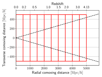
First, we run an $N$-body simulation to obtain the spatial distribution of matter in the Universe at different redshifts. We use Tree-PM code Gadget-2 (Springel, 2005). The number of particles is $2048^{3}$, the volume of the simulation box is $(1\,\mathrm{Gpc}/h)^{3}$, and the corresponding particle mass is $m_{\mathrm{p}}=1.02\times 10^{10}\mathrm{M}_{\odot}/h$. We generate the initial condition at the redshift $z_{\mathrm{ini}}=59$ with a parallel code developed in Nishimichi et al. (2009); Nishimichi et al. (2010); Valageas & Nishimichi (2011), which employs second order Lagrangian perturbation theory. We store 10 snapshots to construct a light-cone output from $z=4.13$ to $z=0.0$. The redshifts at which snapshots are stored are determined to satisfy $\chi(z_{i+1})-\chi(z_{i})=500\,\mathrm{Mpc}/h\ (i=1,\ldots,9)$ and $\chi(z_{1})=250\,\mathrm{Mpc}/h$ (see Figure 1).

Figure 1: Configuration of snapshots. Each red box corresponds to a single snapshot and the dashed lines show the extent of the light-cone. The length in the line-of-sight direction is $500\,\mathrm{Mpc}/h$ and we randomly extract the corresponding region from the original snapshot, which has $1000\,\mathrm{Mpc}/h$ on a side. The dashed lines show the opening angle with $10\,\mathrm{deg}$.

For halo finding, we employ the Rockstar halo finder (Behroozi et al., 2013). We assign gas pressure to each particle which belongs to any halo according to the radius from the center based on the analytic model presented in Section 3.1. If a particle does not belong to any halos, it does not contribute to tSZ signal. Since the code automatically provides the concentration parameter by fitting the density profile with NFW profile, we use this concentration parameter instead of the fitting formula of concentration parameters.

In order to carry out mock observations for WL, we employ the multiple-plane ray-tracing method (White & Hu, 2000; Hamana & Mellier, 2001; Sato et al., 2009; Hilbert et al., 2009). First, we place snapshots to create the light-cone which fills the volume from $z=0$ to $z=4.13$. For each snapshot, we pick $500\,\mathrm{Mpc}/h$ slice, half of the simulation box, in the line-of-sight direction and then randomly rotate and translate particles keeping periodic boundary condition so that the same structure does not appear multiple times. The angular extent of each map is $10\degr\times 10\degr$ and the number of grids on a side is $8192$, which corresponds to the pixel size of $10\degr/8192\simeq 0.073\,\mathrm{arcmin}$. Finally, by repeating the random rotation and translation 100 times, we generate 100 mock $10\degr\times 10\degr$ convergence maps, applying weights derived from the source redshift distribution (Eq. 20).

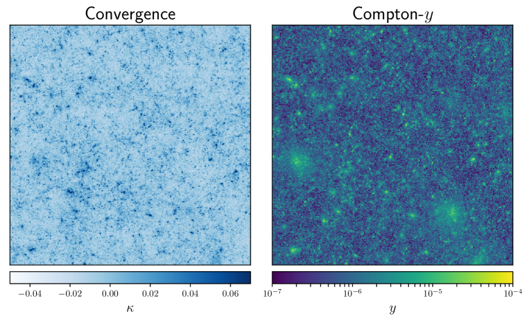
Similarly, we create mock Compton-$y$ maps based on the method presented in Roncarelli et al. (2007); Ursino et al. (2010). For the Compton-$y$ map, we do not include ray deflection effect because the effect is negligible at the scales where measurements are available (Tröster & van Waerbeke, 2014). For sanity check, we measure the average Compton-$y$ parameter $\langle y\rangle$. For the semi-analytic pressure profile, $\langle y\rangle=(1.47\pm 0.10)\times 10^{-6}$ and for the universal pressure profile, $\langle y\rangle=(1.07\pm 0.10)\times 10^{-6}$. The error corresponds to the standard deviation over 100 mock maps. The results are close to that of the previous study (Dolag et al., 2016) based on hydrodynamics simulations, $\langle y\rangle=1.18\times 10^{-6}$. Note that they adopted the different hydrodynamics model and cosmological parameters. For reference, Khatri & Sunyaev (2015) presented bounds of the average Compton-$y$ from which they subtracted the contribution from galaxy clusters as $5.4\times 10^{-8}<\langle y\rangle<2.2\times 10^{-6}$. Figure 2 shows ones of convergence and Compton-$y$ maps as an example.

Figure 2: Convergence and Compton-$y$ maps obtained from simulations. The length on a side corresponds to $10\degr$.

In order to make our simulated maps more realistic, we add noise to convergence and Compton-$y$ maps, and then smooth them with the Gaussian filter. For tSZ maps, following Dolag et al. (2016), we add the Gaussian noise so that the standard deviation of the noise map is $\sigma=1.5\times 10^{-6}$ with the FWHM window scale $\theta_{\mathrm{FWHM}}=10\,\mathrm{arcmin}$. For weak lensing, the dominant source of the noise is the shape noise and the noise can be modeled as Gaussian (van Waerbeke, 2000). The variance of the noise is given as,

$$\sigma^{2}=\frac{\sigma^{2}_{\epsilon}}{\theta^{2}_{\mathrm{pix}}n_{\mathrm{gal}}},$$ (32)

where $\sigma_{\epsilon}$ is the standard deviation of the intrinsic ellipticity, $\theta_{\mathrm{pix}}$ is the pixel size of the map and the $n_{\mathrm{gal}}$ is the mean number density of the source galaxy. For RCSLenS, we adopt $\sigma_{\epsilon}=0.277$ and $n_{\mathrm{gal}}=5.8\,\mathrm{arcmin}^{-2}$ (Hojjati et al., 2017). After adding the noise, both of the maps are smoothed with the Gaussian filter with $\theta_{\mathrm{FWHM}}=10\,\mathrm{arcmin}$ which is the same smoothing scale in creating Compton-$y$ map (Planck Collaboration, 2016b).

3.3 Estimation of the covariance matrix

We present how we measure the covariance matrix from the mock maps generated from simulations. In our analysis, the data vector $\bm{N}$ is defined as,

$$\bm{N}=(C^{yy}(\ell_{1}),\ldots,C^{yy}(\ell_{n_{C}}),\xi^{y\kappa}(\theta_{1}),\ldots,\xi^{y\kappa}(\theta_{n_{\xi}}))^{\mathrm{T}},$$ (33)

where the dimensions of the data vectors are $n_{C}=13\,(52.5\leq\ell\leq 1247.5)$ and $n_{\xi}=8\,(2.55\leq\theta/\mathrm{arcmin}\leq 160)$. Though in Planck data, there are more available data points for lower multipoles, we do not use these data points due to the size of mock maps. We have 100 mock maps and as a result $R=100$ measurement of the data vector $\bm{N}^{r}\,(r=1,\ldots,R)$. The area of mock maps is $100\,\mathrm{deg}^{2}$, but we will apply this covariance matrix to the measurements by Planck and RCSLenS, both of which have larger survey areas. We need to scale the covariance matrix according to the survey area. The estimated covariance matrix is expressed as,

$$\mathrm{Cov}_{ij}=f^{s}_{ij}\frac{1}{R-1}\sum_{r=1}^{R}(N_{i}^{r}-\bar{N}_{i})(N_{j}^{r}-\bar{N}_{j}),$$ (34)

where $\bar{N}$ is the mean over the $R$ realizations,

$$\bar{\bm{N}}=\frac{1}{R}\sum_{r=1}^{R}\bm{N}^{r},$$ (35)

and $f^{s}_{ij}$ is the scaling factor of the survey area,

$$f^{s}_{ij}=\begin{cases}A_{\mathrm{sim}}/A_{\mathrm{Planck}}&(\text{between the power spectrum})\\ A_{\mathrm{sim}}/A_{\mathrm{RCSLenS}}&(\text{between the cross-correlation}).\end{cases}$$ (36)

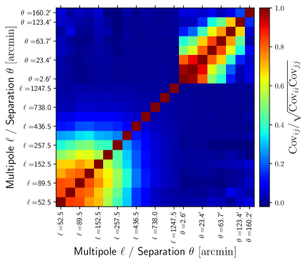
The survey areas are $A_{\mathrm{sim}}=100\,\mathrm{deg}^{2}$, $A_{\mathrm{Planck}}=20626\,\mathrm{deg}^{2}$ and $A_{\mathrm{RCSLenS}}=560\,\mathrm{deg}^{2}$. For covariance between the power spectrum and the cross-correlation, there is no appropriate scaling factor because the sizes of the survey areas of Planck and RCSLenS are different. In order to estimate the cross-covariance, we generate 100 Gaussian maps of Compton-$y$ and convergence which reproduce the power spectrum $C^{yy}(\ell)$ and cross-spectra $C^{y\kappa}(\ell)$ computed from the halo model with the fiducial parameters. The size of Gaussian maps is matched with the survey area of Planck (RCSLenS) for Compton-$y$ (convergence) maps. Then, we compute the power spectra and the cross-correlations based on these maps, and estimate the cross-covariance as the variance over 100 Gaussian maps. For the power spectrum of tSZ, we take into account the variance due to incomplete separation between the signal of tSZ and contaminants, e.g., cosmic infrared background. In order to estimate the variance, we use the values reported by Planck Collaboration (2016b). In Figure 3, the covariance matrices measured from our simulations and Gaussian maps are shown. For the power spectrum part, though mainly the diagonal components are dominated, there are substantial off-diagonal correlations caused by the connected trispectrum term (Horowitz & Seljak, 2017).

Figure 3: Covariance matrices measured from simulations and Gaussian maps. From 1st to 13th rows and columns correspond to the power spectra, and from 14th to 21st rows and columns do to cross-correlations. The upper left (lower left) part corresponds to the covariance with the analytic (observed) pressure profile. The scaling factor due to the size of areas has already been applied.

4 Results

4.1 Power spectrum and cross-correlation

Figure 4: Power spectra of Compton-$y$ from simulations, the halo model prediction of two different pressure profile. The dashed (dot-dashed) line shows 1-halo (2-halo) contribution. The lower panel shows the ratio of 2-halo term to the total spectrum. For comparison, the observational estimates from Planck (Planck Collaboration, 2016b), ACT (Sievers et al., 2013), and SPT (George et al., 2015). are also shown. The shaded region corresponds to the standard deviation over 100 mock maps which cover $100$ square degrees.

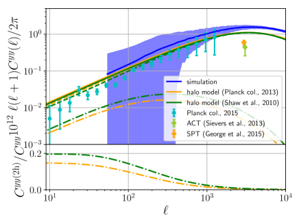
We show power spectra of Compton-$y$ for different models in Figure 4. The results of the analytic model (Shaw et al., 2010) and the simulation based semi-analytic model are not consistent at smaller scales ($\ell\lower 2.15277pt\hbox{$\;\buildrel>\over{\sim}\;$}2000$) possibly due to the lack of resolution in $N$-body simulations. In addition, the effects of the asphericity and substructures can explain part of the differences (Battaglia et al., 2012). However, at scales which can be accessible by Planck data ($100\lower 2.15277pt\hbox{$\;\buildrel<\over{\sim}\;$}\ell\lower 2.15277pt\hbox{$\;\buildrel<\over{\sim}\;$}1000$), both models give consistent results. For even larger scales ($\ell\lower 2.15277pt\hbox{$\;\buildrel<\over{\sim}\;$}100$), the power spectra of the semi-analytic model is suppressed and the variance is quite large affected by the size of mock maps. Overall, all of the results overestimate the power spectrum compared with the measurement of Planck. One of the possible reasons is that our input parameter $\sigma_{8}=0.831$ is high. We will address this point in the following Section.

Figure 5: Cross-correlation function of tSZ and WL from our simulation and halo model calculations. The dashed (dot-dashed) line shows 1-halo (2-halo) contribution. The lower panel shows the ratio of 2-halo term to the total cross-correlation. The shaded region corresponds to the standard deviation over 100 mock maps which cover $100$ square degrees.

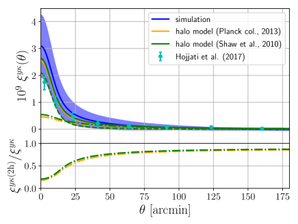
Figure 5 shows the cross-correlation of tSZ and WL from our simulation based semi-analytic model and halo model calculations. Although the excess of the cross-correlations at small scales ($\theta<10\,\mathrm{arcmin}$) can be seen as a possible tension, the results are consistent with each other on larger scales. This difference also can be induced by the high value of $\sigma_{8}$.

4.2 Constraints on non-thermal pressure and $\sigma_{8}$

With the power spectrum and the cross-correlation measured by Planck and RCSLenS, we can constrain the amplitude $\alpha_{0}$ of the non-thermal pressure and the amplitude of the matter power spectrum, i.e., $\sigma_{8}$. Other model parameters and cosmological parameters are fixed at the fiducial values. The posterior distribution when both of the power spectrum and the cross-correlation are used is given as,

$$\log L(\alpha_{0},\sigma_{8}|\bm{N}_{\mathrm{data}})=-\frac{1}{2}\log[(2\pi)^{n_{C}+n_{\xi}}|\det\mathrm{Cov}|]$$

$$-\frac{1}{2}(\bm{N}_{\mathrm{data}}-\bm{N}_{\mathrm{model}})^{\mathrm{T}}(\mathrm{Cov})^{-1}(\bm{N}_{\mathrm{data}}-\bm{N}_{\mathrm{model}}),$$ (37)

where $\bm{N}_{\mathrm{data}}=(\bm{C}^{yy}_{\mathrm{Planck}},\bm{\xi}^{y\kappa}_{\mathrm{RCSLenS}})$ and $\bm{N}_{\mathrm{model}}$ is the halo model prediction given $\alpha_{0}$ and $\sigma_{8}$. When we use either the power spectrum or the cross-correlation, we simply use a submatrix of the covariance and a subvector of the model vector.

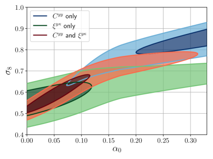
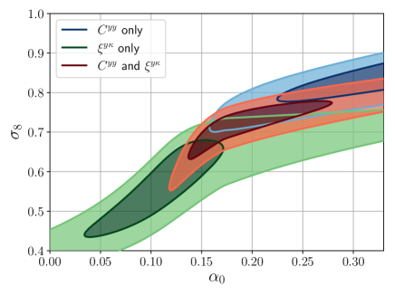
We estimate the probability contours by computing the posterior probability at regular grids. The posterior distribution is shown in Figure 6 with different data sets, power spectrum only, cross-correlation only, both of them. The red, blue, and green solid lines correspond to the confidence regions with the data sets of both of power spectra and cross-correlations, power spectra only, and cross-correlations only, respectively. With all data sets, the clear degeneracy between $\sigma_{8}$ and $\alpha_{0}$ can be seen. If only the power spectra are employed, moderate $\sigma_{8}\sim 0.85$ are preferred but the estimated $\alpha_{0}$ is clearly larger than the fiducial value $0.18$. On the other hand, the results with cross-correlations (red and green lines) prefer low $\sigma_{8}\sim 0.6$ and low $\alpha_{0}\sim 0.05$. The low non-thermal pressure amplitude $\alpha_{0}$ is strongly inconsistent with the predictions based on hydrodynamical cosmological simulations (Shaw et al., 2010; Nelson et al., 2014). The estimated value of $\sigma_{8}$ is quite smaller than the result from CMB measurements of Planck, $\sigma_{8}=0.831\pm 0.013$ (TT,TE,EE+lowP, Planck Collaboration, 2016a). However, recent analysis of KiDS weak lensing survey (Köhlinger et al., 2017) reports $\sigma_{8}\sqrt{\Omega_{\mathrm{m}}/0.3}=0.651\pm 0.058$, i.e. $\sigma_{8}=0.635\pm 0.057$ for $\Omega_{\mathrm{m}}=0.3156$, which is consistent with our result within $1\sigma$ level.

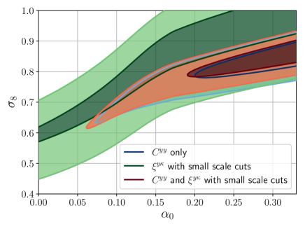
In addition, we investigate the effect of the small scale (less than $10\,\mathrm{arcmin}$, which is the smoothing scale) cross-correlations. Figure 7 shows the confidence regions with small scale cross-correlations excluded. In these cases, all of results become consistent with each other. This result indicates that the tension originates from the small scales.

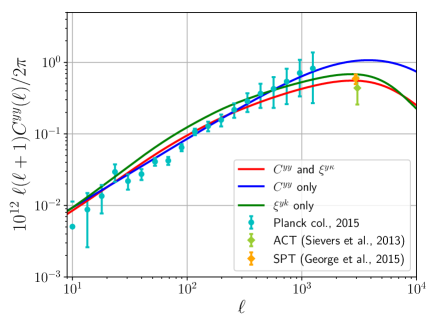
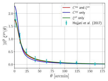
In Figure 8 we show the tSZ power spectrum and tSZ-WL cross-correlation, together with the best-fit model parameters estimated with the data sets of power spectrum only, cross-correlation only, and both. Remarkably, when we include cross-correlations, the best-fit power spectrum can reproduce ACT and SPT data points, though these data points are not used in the analysis.

Figure 6: Posterior distributions of non-thermal pressure parameters $\alpha_{0}$ and $\sigma_{8}$. The inner (outer) colored region correponds to $1\sigma$ ($2\sigma$) confidence level. The results with data sets of power spectra and cross-correlations, power spectra only, and cross-correlations are shown in solid red, blue, and green regions, respectively.

Figure 7: Posterior distributions of non-thermal pressure parameters $\alpha_{0}$ and $\sigma_{8}$ with small scale ($<10\,\mathrm{arcmin}$) cuts in cross-correlations. The inner (outer) colored region correponds to $1\sigma$ ($2\sigma$) confidence level. The results with data sets of power spectra and cross-correlations, power spectra only, and cross-correlations only are shown in solid red, blue, and green regions, respectively. Note that the blue regions are identical in Figure 6 because this data set does not include cross-correlations.

Figure 8: Power spectra and cross-correlations with best-fit parameters. The results using data sets of power spectra only, cross-correlations only, and both are shown as blue, green, and red lines, respectively.

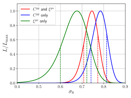
We next derive constraints on $\sigma_{8}$ using the universal pressure profile with parameters calibrated against Planck data (Eq. 29). Note that we apply the pressure profile to less massive and/or high redshift halos, which are not calibrated in this pressure profile. Using only the tSZ power spectrum data, we find $\sigma_{8}=0.785^{+0.029}_{-0.043}$, consistent with Planck Collaboration (2016b), who find $\sigma_{8}(\Omega_{\mathrm{m}}/0.28)^{3/8}=0.80^{+0.01}_{-0.03}$, i.e., $\sigma_{8}=0.76^{+0.01}_{-0.03}$ for $\Omega_{\mathrm{m}}=0.3156$, from a similar analysis. The tSZ-WL cross-correlation on the other hand prefers a lower value of $\sigma_{8}=0.677^{+0.046}_{-0.077}$. Combining the two data sets, we find $\sigma_{8}=0.746^{+0.026}_{-0.038}$. The posterior distributions derived from tSZ and the tSZ-WL cross-correlation show a clear tension (see Fig. 9).

Figure 9: Posterior distributions of $\sigma_{8}$ with the power spectrum and the cross-correlation using the observationally calibrated universal pressure profile. The dashed lines show the $16\%$ and $84\%$ percentile.

Table 1: Summary of constraints on $\sigma_{8}$. The best-fit value and $16\%$ and $84\%$ percentile values are shown.

Data sets	Constraints of $\sigma_{8}$
$C^{yy}$ and $\xi^{y\kappa}$	$0.746^{+0.026}_{-0.038}$
$C^{yy}$ only	$0.785^{+0.029}_{-0.043}$
$\xi^{y\kappa}$ only	$0.677^{+0.046}_{-0.077}$

4.3 Mitigating the tension between the data sets

As seen above, the constraints on $\sigma_{8}$ and $\alpha_{0}$ from the tSZ power spectrum and the tSZ-WL cross-correlation are inconsistent. The tension seems to originate from the small scales, as we have seen in Figure 7. Here, we investigate if modifications to the gas model can help mitigate the tension. The analytic pressure profile is calibrated against X-ray observations of massive clusters over a wide range of redshift, and low redshift galaxy groups (Flender et al., 2017). Therefore, the gas profile of galaxy groups at high redshift is not calibrated in the current framework.

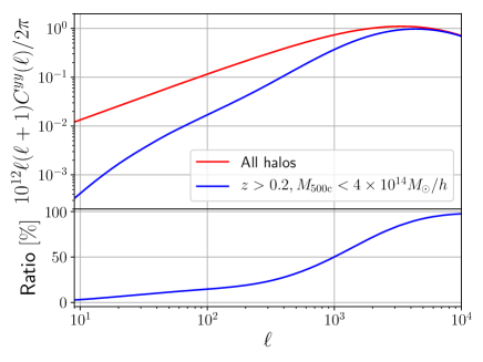
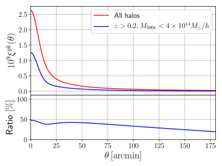
High-redshift, low-mass groups and clusters contribute a considerable fraction to the total tSZ power spectrum and tSZ-WL cross-correlation, as shown in Figure 10, where we show the contribution from objects with $z>0.2$ and $M_{\mathrm{500c}}<4\times 10^{14}\mathrm{M}_{\odot}/h$. These objects contribute around $50\%$ to the measured tSZ-WL cross-correlation, and $50\%$–$100\%$ to the tSZ power spectrum at $1000<\ell<10000$. At multipoles probed by Planck ($50\lower 2.15277pt\hbox{$\;\buildrel<\over{\sim}\;$}\ell\lower 2.15277pt\hbox{$\;\buildrel<\over{\sim}\;$}1000$), they contribute still $\sim 10\%$–$50\%$.

Figure 10: Contributions of the power spectrum and cross-correlation from high redshift groups ($z>0.2$ and $M_{\mathrm{500c}}<4\times 10^{14}\mathrm{M}_{\odot}/h$). The lower panels show the fraction with respect to contributions from all halos

In order to mitigate the tension between data sets, we consider the case of varying a parameter, $S_{*}$, which is the power index of the stellar-to-halo-mass relation defined in Eq. 28. When we take high $S_{*}$, the gas fraction reduces especially for group size halos, and then the resultant power spectra and cross-correlations are suppressed. To demonstrate that the high $S_{*}$ model has a possibility to alleviate the tension, we repeat our analysis with $S_{*}=0.7$. In this case, we find that the tension between the two data sets, the tSZ power spectrum and tSZ-WL cross-correlation, is mitigated (see Figure 11). Both data sets are consistent with the fiducial value $\alpha_{0}=0.18$.

We note that the high value for the slope in the stellar fraction, $S_{*}=0.7$, is inconsistent with the results from Flender et al. (2017), who find $S_{*}=0.12\pm 0.1$. On the other hand, the steep slope is consistent with the results from Gonzalez et al. (2007), who analyze the stellar content of groups and clusters over a wide range of masses, $6\times 10^{13}$–$10^{15}\mathrm{M}_{\odot}$, and find $S_{*}=0.64\pm 0.13$.

We have also tried other modification to the gas model in order to mitigate the tension, varying $f_{*}$, $\epsilon_{\mathrm{f}}$, or introducing an additional redshift dependence to the tSZ signal, but found that enhanced star formation due to high $S_{*}$ works best, since it has the most impact on small scales, where the tension originates.

Figure 11: Posterior distributions of non-thermal pressure parameters $\alpha_{0}$ and $\sigma_{8}$ with $S_{*}=0.7$. The inner (outer) colored region correponds to $1\sigma$ ($2\sigma$) confidence region. The results with data sets of power spectra and cross-correlations, power spectra only, and cross-correlations only are shown in solid red, blue, and green regions, respectively.

5 Conclusions

The tSZ effect probes the thermal properties of the hot, ionized gas in the Universe, while the WL signal reflects mostly the dark matter distribution, and is thus less affected by baryonic physics. Current and future CMB and galaxy redshift surveys enable measurements of these observables, which can be used to infer astrophysical and cosmological information. The first detections of the tSZ-WL cross-correlation have been recently reported in van Waerbeke et al. (2014); Hill & Spergel (2014); Hojjati et al. (2017). The cross-correlation can be a valuable probe in addition to tSZ and WL alone, as it can help break parameter degeneracies.

In this work, we have modeled the tSZ-WL cross-correlation using the halo model approach. We have modeled the pressure profile following the semi-analytic ICM model from Flender et al. (2017), as well as the universal pressure profile calibrated against observations (Planck Collaboration, 2013). In order to estimate the covariance matrix, we have produced mock tSZ and WL maps. For WL, we employ the ray-tracing technique to generate mock maps of the convergence field. For tSZ, we follow the approach from Roncarelli et al. (2007), painting the signal into the halos in the simulation.

We constrain the free parameters in our model, taking into account measurements of the tSZ power spectrum from Planck (Planck Collaboration, 2016b), as well as measurements of the tSZ-WL cross-correlation from RCSLenS and Planck (Hojjati et al., 2017). With the observationally calibrated universal pressure profile from Planck Collaboration (2013), and leaving $\sigma_{8}$ as the only free parameter, we find that the tSZ data alone prefers $\sigma_{8}=0.785^{+0.029}_{-0.043}$, consistent with the value of 0.76 found in Planck Collaboration (2016b). However, the value for $\sigma_{8}$ becomes lower when taking into account the tSZ-WL cross-correlation. With the cross-correlation alone we find $\sigma_{8}=0.677^{+0.046}_{-0.077}$, and with the combined data $\sigma_{8}=0.746^{+0.026}_{-0.038}$.

We repeat the analysis using the pressure profile from the semi-analytic model from Flender et al. (2017), leaving the amplitude of non-thermal pressure, $\alpha_{0}$, and $\sigma_{8}$ as free parameters. Here, we find that the tSZ power spectrum prefers $\alpha_{0}\sim 0.3$ and $\sigma_{8}\sim 0.85$, while the tSZ-WL cross-correlation prefers a significantly lower $\alpha_{0}$ of $\sim 0.05$ and $\sigma_{8}\sim 0.6$ (see Figure 6). Ignoring the small scales ($<10\,\mathrm{arcmin}$) in the analysis seems to alleviate the tension (see Figure 7).

Another way to alleviate the tension between the two data sets is to consider modifications in the gas model. We find that allowing for a steep slope in the stellar-mass-halo-mass relation, $S_{*}=0.7$, results in posterior distributions from the two data sets that are less in tension (see Figure 11), pointing towards enhanced star formation in low-mass halos. With the combined data, we find that a model with $\sigma_{8}\sim 0.7$, $\alpha_{0}\sim 0.2$ is preferred.

The tSZ power spectrum and the tSZ-WL cross-correlation are exciting new probes of cluster astrophysics and cosmology. Upcoming galaxy redshift surveys, such as HSC and LSST, and CMB experiments, such as ACTPol, SPT-3G, and CMB-Stage IV, will enable more precise measurements of these observables, especially at smaller scales than the $\sim 10\,\mathrm{arcmin}$ size of the Planck beam, which currently limits our analysis. Considering the high quality and wide coverage of future data, semi-analytic modeling in combination with all-sky simulations (Shirasaki et al., 2015) will be a promising modeling approach. If future data confirm the tension seen here with higher significance, we might derive interesting conclusions about the gas physics of groups and clusters, such as enhanced star formation, i.e. reduced gas content in low-mass halos. Another possibility would be to derive constraints on the shape of the pressure profile (see, Battaglia et al., 2017).

Appendix A Summary of symbols

In Table 2, we summarize symbols used in this paper.

Table 2: Symbols used in this paper.

Symbol	Definition	Reference equation
	Halo model
$y$	Compton-$y$	(1)
$P_{\mathrm{e}}$	Free electron pressure	(1)
$C^{yy}(\ell)$	Power spectrum of Compton-$y$	(4)
$C^{yy\mathrm{(1h)}}(\ell)$	1-halo term of $C^{yy}(\ell)$	(5)
$C^{yy\mathrm{(2h)}}(\ell)$	2-halo term of $C^{yy}(\ell)$	(6)
$y_{\ell}$	Fourier transform of Compton-$y$ of single halo	(6)
$dn/dM$	Halo mass function	(5), (6)
$b$	Halo bias	(6)
$P_{\mathrm{m}}(k,z)$	Linear matter power spectrum	(6)
$M_{\Delta}$	Halo mass with the overdensity $\Delta$	(8)
$M_{500\mathrm{c}}$	Halo mass with the overdensity $\Delta=500$	…
$M_{\mathrm{vir}}$	Virial halo mass	(9), (16)
$\rho(r)$	Density profile of halo	(15)
$c(M_{\mathrm{vir}},z)$	Concentration parameter	(18)
$\kappa$	Weak lensing convergence	…
$\kappa_{\ell}$	Fourier transform of convergence of single halo	(19)
$C^{y\kappa}(\ell)$	Cross power spectrum of Compton-$y$ and convergence	(12)
$C^{y\kappa\mathrm{(1h)}}(\ell)$	1-halo term of $C^{y\kappa}(\ell)$	(13)
$C^{y\kappa\mathrm{(2h)}}(\ell)$	2-halo term of $C^{y\kappa}(\ell)$	(14)
$\xi^{y\kappa}(\theta)$	Cross correlation function of Compton-$y$ and convergence	(21)
	Semi-analytic model of the ICM
$P_{\mathrm{tot}}(r)$	Total pressure profile of halo	(22), (23)
$P_{\mathrm{nt}}(r)$	Non-thermal pressure profile of halo	(26)
$\rho_{g}(r)$	Gas density profile of halo	(22), (24)
$\alpha(z)$	Amplitude of radial profile of non-thermal fraction	(26), (27)
$n_{\mathrm{nt}}$	Power law index of non-thermal fraction	(26)
$\alpha_{0}$	Amplitude of $\alpha(z)$	(27)
$\beta$	Parameter which determines redshift dependence of $\alpha(z)$	(27)
$\epsilon_{\mathrm{DM}}$	Parameter which describes energy transfer between dark matter and gas	…
$\epsilon_{\mathrm{f}}$	Parameter which regulates stellar feedback energy	…
$f_{*}$	Amplitude of stellar mass fraction relation	(28)
$S_{*}$	Power law index of stellar mass fraction relation	(28)

References

- Aihara et al. (2017) Aihara H., et al., 2017, preprint, (arXiv:1704.05858)
- Arnaud et al. (2010) Arnaud M., Pratt G. W., Piffaretti R., Böhringer H., Croston J. H., Pointecouteau E., 2010, Astronomy and Astrophysics, 517, A92
- Austermann et al. (2012) Austermann J. E., et al., 2012, Millimeter, Submillimeter, and Far-Infrared Detectors and Instrumentation for Astronomy VI. Proceedings of the SPIE, 8452
- Bartelmann & Schneider (2001) Bartelmann M., Schneider P., 2001, Physics Reports, 340, 291
- Battaglia et al. (2010) Battaglia N., Bond J. R., Pfrommer C., Sievers J. L., Sijacki D., 2010, The Astrophysical Journal, 725, 91
- Battaglia et al. (2012) Battaglia N., Bond J. R., Pfrommer C., Sievers J. L., 2012, The Astrophysical Journal, 758, 75
- Battaglia et al. (2015) Battaglia N., Hill J. C., Murray N., 2015, The Astrophysical Journal, 812, 154
- Battaglia et al. (2017) Battaglia N., Ferraro S., Schaan E., Spergel D., 2017, preprint, (arXiv:1705.05881)
- Battye et al. (2015) Battye R. A., Charnock T., Moss A., 2015, Phys. Rev. D, 91, 103508
- Behroozi et al. (2013) Behroozi P. S., Wechsler R. H., Wu H.-Y., 2013, The Astrophysical Journal, 762, 109
- Birkinshaw (1999) Birkinshaw M., 1999, Physics Reports, 310, 97
- Bleem et al. (2015) Bleem L. E., et al., 2015, The Astrophysical Journal Supplement, 216, 27
- Bocquet et al. (2016) Bocquet S., Saro A., Dolag K., Mohr J. J., 2016, Monthly Notices of the Royal Astronomical Society, 456, 2361
- Bryan & Norman (1998) Bryan G. L., Norman M. L., 1998, The Astrophysical Journal, 495, 80
- Carlstrom et al. (2002) Carlstrom J. E., Holder G. P., Reese E. D., 2002, Annual Review of Astronomy and Astrophysics, 40, 643
- Carlstrom et al. (2011) Carlstrom J. E., et al., 2011, Publications of the Astronomical Society of Pacific, 123, 568
- Cole & Kaiser (1988) Cole S., Kaiser N., 1988, Monthly Notices of the Royal Astronomical Society, 233, 637
- Dark Energy Survey Collaboration (2016) Dark Energy Survey Collaboration 2016, Monthly Notices of the Royal Astronomical Society, 460, 1270
- Dolag et al. (2016) Dolag K., Komatsu E., Sunyaev R., 2016, Monthly Notices of the Royal Astronomical Society, 463, 1797
- Duffy et al. (2008) Duffy A. R., Schaye J., Kay S. T., Dalla Vecchia C., 2008, Monthly Notices of the Royal Astronomical Society Letters, 390, L64
- Flender et al. (2017) Flender S., Nagai D., McDonald M., 2017, The Astrophysical Journal, 837, 124
- George et al. (2015) George E. M., et al., 2015, The Astrophysical Journal, 799, 177
- Gonzalez et al. (2007) Gonzalez A. H., Zaritsky D., Zabludoff A. I., 2007, The Astrophysical Journal, 666, 147
- Hamana & Mellier (2001) Hamana T., Mellier Y., 2001, Monthly Notices of the Royal Astronomical Society, 327, 169
- Harnois-Déraps et al. (2016) Harnois-Déraps J., et al., 2016, Monthly Notices of the Royal Astronomical Society, 460, 434
- Hasselfield et al. (2013) Hasselfield M., et al., 2013, Journal of Cosmology and Astroparticle Physics, 7, 008
- Hilbert et al. (2009) Hilbert S., Hartlap J., White S. D. M., Schneider P., 2009, Astronomy and Astrophysics, 499, 31
- Hildebrandt et al. (2016) Hildebrandt H., et al., 2016, Monthly Notices of the Royal Astronomical Society, 463, 635
- Hill & Spergel (2014) Hill J. C., Spergel D. N., 2014, Journal of Cosmology and Astroparticle Physics, 02, 030
- Hojjati et al. (2015) Hojjati A., McCarthy I. G., Harnois-Deraps J., Ma Y.-Z., Waerbeke L. V., Hinshaw G., Brun A. M. L., 2015, Journal of Cosmology and Astroparticle Physics, 10, 047
- Hojjati et al. (2017) Hojjati A., et al., 2017, MNRAS, 471, 1565
- Horowitz & Seljak (2017) Horowitz B., Seljak U., 2017, Monthly Notices of the Royal Astronomical Society, 469, 394
- Itoh et al. (1998) Itoh N., Kohyama Y., Nozawa S., 1998, The Astrophysical Journal, 502, 7
- Khatri & Sunyaev (2015) Khatri R., Sunyaev R., 2015, J. Cosmology Astropart. Phys., 8, 013
- Kilbinger (2015) Kilbinger M., 2015, Reports on Progress in Physics, 78, 086901
- Kitayama (2014) Kitayama T., 2014, Progress of Theoretical and Experimental Physics, 2014, 6B111
- Köhlinger et al. (2017) Köhlinger F., et al., 2017, MNRAS, 471, 4412
- Komatsu & Kitayama (1999) Komatsu E., Kitayama T., 1999, The Astrophysical Journal, 526, L1
- Komatsu & Seljak (2001) Komatsu E., Seljak U., 2001, Monthly Notices of the Royal Astronomical Society, 327, 1353
- Komatsu & Seljak (2002) Komatsu E., Seljak U., 2002, Monthly Notices of the Royal Astronomical Society, 336, 1256
- LSST Science Collaboration (2009) LSST Science Collaboration 2009, preprint, (arXiv:0912.0201)
- Leauthaud et al. (2017) Leauthaud A., et al., 2017, MNRAS, 467, 3024
- Ma et al. (2015) Ma Y.-Z., Van Waerbeke L., Hinshaw G., Hojjati A., Scott D., Zuntz J., 2015, Journal of Cosmology and Astroparticle Physics, 9, 046
- McCarthy et al. (2014) McCarthy I. G., Le Brun A. M. C., Schaye J., Holder G. P., 2014, Monthly Notices of the Royal Astronomical Society, 440, 3645
- Munshi et al. (2008) Munshi D., Valageas P., van Waerbeke L., Heavens A., 2008, Physics Reports, 462, 67
- Munshi et al. (2014) Munshi D., Joudaki S., Coles P., Smidt J., Kay S. T., 2014, MNRAS, 442, 69
- Nagai et al. (2007) Nagai D., Kravtsov A. V., Vikhlinin A., 2007, The Astrophysical Journal, 668, 1
- Navarro et al. (1996) Navarro J. F., Frenk C. S., White S. D. M., 1996, The Astrophysical Journal, 462, 563
- Navarro et al. (1997) Navarro J. F., Frenk C. S., White S. D. M., 1997, The Astrophysical Journal, 490, 493
- Nelson et al. (2014) Nelson K., Lau E. T., Nagai D., 2014, The Astrophysical Journal, 792, 25
- Niemack et al. (2010) Niemack M. D., et al., 2010, Proceedings of the SPIE, 7741
- Nishimichi et al. (2009) Nishimichi T., et al., 2009, Publications of the Astronomical Society of Japan, 61, 321
- Nishimichi et al. (2010) Nishimichi T., Taruya A., Koyama K., Sabiu C., 2010, Journal of Cosmology and Astroparticle Physics, 07, 002
- Nozawa et al. (1998) Nozawa S., Itoh N., Kohyama Y., 1998, The Astrophysical Journal, 508, 17
- Oguri & Takada (2011) Oguri M., Takada M., 2011, Physical Review D, 83, 023008
- Ostriker et al. (2005) Ostriker J. P., Bode P., Babul A., 2005, The Astrophysical Journal, 634, 964
- Planck Collaboration (2013) Planck Collaboration 2013, Astronomy and Astrophysics, 550, A131
- Planck Collaboration (2016a) Planck Collaboration 2016a, Astronomy and Astrophysics, 594, A13
- Planck Collaboration (2016b) Planck Collaboration 2016b, Astronomy and Astrophysics, 594, A22
- Roncarelli et al. (2007) Roncarelli M., Moscardini L., Borgani S., Dolag K., 2007, Monthly Notices of the Royal Astronomical Society, 378, 1259
- Sato et al. (2009) Sato M., Hamana T., Takahashi R., Takada M., Yoshida N., Matsubara T., Sugiyama N., 2009, The Astrophysical Journal, 701, 945
- Sehgal et al. (2010) Sehgal N., Bode P., Das S., Hernandez-Monteagudo C., Huffenberger K., Lin Y.-T., Ostriker J. P., Trac H., 2010, The Astrophysical Journal, 709, 920
- Shaw et al. (2010) Shaw L. D., Nagai D., Bhattacharya S., Lau E. T., 2010, The Astrophysical Journal, 725, 1452
- Shirasaki et al. (2015) Shirasaki M., Hamana T., Yoshida N., 2015, Monthly Notices of the Royal Astronomical Society, 453, 3043
- Sievers et al. (2013) Sievers J. L., et al., 2013, Journal of Cosmology and Astroparticle Physics, 10, 060
- Springel (2005) Springel V., 2005, Monthly Notices of the Royal Astronomical Society, 364, 1105
- Sunyaev & Zeldovich (1972) Sunyaev R. A., Zeldovich Y. B., 1972, Comments on Astrophysics and Space Physics, 4, 173
- Sunyaev & Zeldovich (1980) Sunyaev R. A., Zeldovich Y. B., 1980, Monthly Notices of the Royal Astronomical Society, 190, 413
- Swetz et al. (2011) Swetz D. S., et al., 2011, The Astrophysical Journal Supplement, 194, 41
- Tinker et al. (2010) Tinker J. L., Robertson B. E., Kravtsov A. V., Klypin A., Warren M. S., Yepes G., Gottlöber S., 2010, The Astrophysical Journal, 724, 878
- Trac et al. (2011) Trac H., Bode P., Ostriker J. P., 2011, The Astrophysical Journal, 727, 94
- Tröster & van Waerbeke (2014) Tröster T., van Waerbeke L., 2014, Journal of Cosmology and Astroparticle Physics, 11, 008
- Ursino et al. (2010) Ursino E., Galeazzi M., Roncarelli M., 2010, The Astrophysical Journal, 721, 46
- Valageas & Nishimichi (2011) Valageas P., Nishimichi T., 2011, Astronomy and Astrophysics, 527, A87
- White & Hu (2000) White M., Hu W., 2000, The Astrophysical Journal, 537, 1
- van Waerbeke (2000) van Waerbeke L., 2000, Monthly Notices of the Royal Astronomical Society, 313, 524
- van Waerbeke et al. (2014) van Waerbeke L., Hinshaw G., Murray N., 2014, Physical Review D, 89, 023508