Exploring Generalization in Deep Learning

Behnam Neyshabur, Srinadh Bhojanapalli, David McAllester, Nathan Srebro
Toyota Technological Institute at Chicago
{bneyshabur, srinadh, mcallester, nati}@ttic.edu
Abstract

With a goal of understanding what drives generalization in deep networks, we consider several recently suggested explanations, including norm-based control, sharpness and robustness. We study how these measures can ensure generalization, highlighting the importance of scale normalization, and making a connection between sharpness and PAC-Bayes theory. We then investigate how well the measures explain different observed phenomena.

1 Introduction

Learning with deep neural networks has enjoyed huge empirical success in recent years across a wide variety of tasks. Despite being a complex, non-convex optimization problem, simple methods such as stochastic gradient descent (SGD) are able to recover good solutions that minimize the training error. More surprisingly, the networks learned this way exhibit good generalization behavior, even when the number of parameters is significantly larger than the amount of training data [19, 29].

In such an over parametrized setting, the objective has multiple global minima, all minimize the training error, but many of them do not generalize well. Hence, just minimizing the training error is not sufficient for learning: picking the wrong global minima can lead to bad generalization behavior. In such situations, generalization behavior depends implicitly on the algorithm used to minimize the training error. Different algorithmic choices for optimization such as the initialization, update rules, learning rate, and stopping condition, will lead to different global minima with different generalization behavior [6, 11, 17]. For example, Neyshabur et al. [17] introduced Path-SGD, an optimization algorithm that is invariant to rescaling of weights, and showed better generalization behavior over SGD for both feedforward and recurrent neural networks [17, 21]. Keskar et al. [11] noticed that the solutions found by stochastic gradient descent with large batch sizes generalizes worse than the one found with smaller batch sizes, and Hardt et al. [9] discuss how stochastic gradient descent ensures uniform stability, thereby helping generalization for convex objectives.

What is the bias introduced by these algorithmic choices for neural networks? What ensures generalization in neural networks? What is the relevant notion of complexity or capacity control?

As mentioned above, simply accounting for complexity in terms of the number of parameters, or any measure which is uniform across all functions representable by a given architecture, is not sufficient to explain the generalization ability of neural networks trained in practice. For linear models, norms and margin-based measures, and not the number of parameters, are commonly used for capacity control  [4, 8, 24]. Also norms such as the trace norm and max norm are considered as sensible inductive biases in matrix factorization and are often more appropriate than parameter-counting measures such as the rank [26, 27]. In a similar spirit, Bartlett [2] and later Neyshabur et al. [19] suggested different norms of network parameters to measure the capacity of neural networks. In a different line of work, Keskar et al. [11] suggested “sharpness” (robustness of the training error to perturbations in the parameters) as a complexity measure for neural networks. Others, including Langford and Caruana [12] and more recently Dziugaite and Roy [7], propose a PAC-Bayes analysis.

What makes a complexity measure appropriate for explaining generalization in deep learning? First, an appropriate complexity measure must be sufficient in ensuring generalization. Second, networks learned in practice should be of low complexity under this measure. This can happen if our optimization algorithms bias us toward lower complexity models under this measure and it is possible to capture real data using networks of low complexity. In particular, the complexity measure should help explain several recently observed empirical phenomena that are not explained by a uniform notion of complexity:

  • It is possible to obtain zero training error on random labels using the same architecture for which training with real labels leads to good generalization [29]. We would expect the networks learned using real labels (and which generalizes well) to have much lower complexity, under the suggested measure, than those learned using random labels (and which obviously do not generalize well).

  • Increasing the number of hidden units, thereby increasing the number of parameters, can lead to a decrease in generalization error even when the training error does not decrease [19]. We would expect to see the complexity measure decrease as we increase the number of hidden units.

  • When training the same architecture, with the same training set, using two different optimization methods (or different algorithmic or parameter choices), one method results in better generalization even though both lead to zero training error [17, 11]. We would expect to see a correlation between the complexity measure and generalization ability among zero-training error models.

In this paper we examine different complexity measures that have recently been suggested, or could be considered, in explaining generalization in deep learning. In light of the above, we evaluate the measures based on their ability to theoretically guarantee generalization, and their empirical ability to explain the above phenomena. Studying how each measure can guarantee generalization also let us better understand how it should be computed and compared when trying to explain the empirical phenomena.

We investigate complexity measures including norms, robustness and sharpness of the network. We emphasize in our theoretical and empirical study the importance of relating the scale of the parameters and the scale of the output of the network, e.g. by relating norm and margin. In this light, we discuss how sharpness by itself is not sufficient for ensuring generalization, but can be combined, through PAC-Bayes analysis, with the norm of the weights to obtain an appropriate complexity measure. The role of sharpness in PAC-Bayesian analysis of neural networks was also recently noted by Dziugaite and Roy [7], who used numerical techniques to numerically optimize the overall PAC-Bayes bound—here we emphasize the distinct role of sharpness as a balance for norm.

In order to further understand the significance of sharpness in deep learning, and how its relationship to margin deviates for that found in linear models, we also establish, in Section 4, sufficient conditions on the network that provably ensures small sharpness.

Notation

Let f𝐰(𝐱)subscript𝑓𝐰𝐱f_{\mathbf{w}}(\mathbf{x}) be the function computed by a d𝑑d layer feed-forward network with parameters 𝐰𝐰\mathbf{w} and Rectified Linear Unit (ReLU) activations, f𝐰(𝐱)=Wdϕ(Wd1ϕ(.ϕ(W1𝐱)))f_{\mathbf{w}}(\mathbf{x})=W_{d}\,\phi(W_{d-1}\,\phi(....\phi(W_{1}\mathbf{x}))) where ϕ(z)=max{0,z}italic-ϕ𝑧0𝑧\phi(z)=\max\{0,z\}. For a given 𝐱n𝐱superscript𝑛\mathbf{x}\in\mathbb{R}^{n}, let Di𝐱,𝐰subscriptsuperscript𝐷𝐱𝐰𝑖D^{\mathbf{x},\mathbf{w}}_{i} denote the diagonal {1,0}10\{1,0\} matrix corresponding to activation in layer i𝑖i. To simplify the presentation we drop the 𝐱𝐱\mathbf{x} superscript and use Disubscript𝐷𝑖D_{i} instead. We can therefore write f𝐰(𝐱)=WdDd1Wd1D1W1𝐱=Wd(Πi=1d1DiWi)𝐱subscript𝑓𝐰𝐱subscript𝑊𝑑subscript𝐷𝑑1subscript𝑊𝑑1subscript𝐷1subscript𝑊1𝐱subscript𝑊𝑑superscriptsubscriptΠ𝑖1𝑑1subscript𝐷𝑖subscript𝑊𝑖𝐱f_{\mathbf{w}}(\mathbf{x})=W_{d}\,D_{d-1}\,W_{d-1}\,\cdots\,D_{1}\,W_{1}\,\mathbf{x}=W_{d}\left(\Pi_{i=1}^{d-1}D_{i}W_{i}\right)\mathbf{x} where we drop the 𝐱,𝐰𝐱𝐰{\mathbf{x},\mathbf{w}} superscript from Di𝐱,𝐰superscriptsubscript𝐷𝑖𝐱𝐰D_{i}^{\mathbf{x},\mathbf{w}} and use Disubscript𝐷𝑖D_{i} instead but remember that Disubscript𝐷𝑖D_{i} depends on 𝐱𝐱\mathbf{x} and the parameters Wjsubscript𝑊𝑗W_{j} for any ji𝑗𝑖j\leq i.

Let hisubscript𝑖h_{i} be the number of nodes in layer i𝑖i, with h0=nsubscript0𝑛h_{0}=n. Therefore, for any layer i𝑖i, we have WiRhi×hi1subscript𝑊𝑖superscript𝑅subscript𝑖subscript𝑖1W_{i}\in R^{h_{i}\times h_{i-1}}. Given any input x𝑥x, the loss of the prediction by the function f𝐰subscript𝑓𝐰f_{\mathbf{w}} is then given by (𝐰,𝐱)𝐰𝐱\ell(\mathbf{w},\mathbf{x}). We also denote by L(𝐰)𝐿𝐰L(\mathbf{w}) the expected loss and by L^(𝐰)^𝐿𝐰\widehat{L}(\mathbf{w}) the empirical loss over the training set. For any integer k𝑘k, [k]delimited-[]𝑘[k] denotes the set {1,2,,k}12𝑘\{1,2,\cdots,k\}. Finally, .F\left\lVert{.}\right\rVert_{F}, .2\left\lVert{.}\right\rVert_{2}, .1\left\lVert{.}\right\rVert_{1}, .\left\lVert{.}\right\rVert_{\infty} denote Frobenius norm, the spectral norm, element-wise 1subscript1\ell_{1}-norm and element-wise subscript\ell_{\infty} norm respectively.

2 Generalization and Capacity Control in Deep Learning

In this section, we discuss complexity measures that have been suggested, or could be used for capacity control in neural networks. We discuss advantages and weaknesses of each of these complexity measures and examine their abilities to explain the observed generalization phenomena in deep learning.

We consider the statistical capacity of a model class in terms of the number of examples required to ensure generalization, i.e. that the population (or test error) is close to the training error, even when minimizing the training error. This also roughly corresponds to the maximum number of examples on which one can obtain small training error even with random labels.

Given a model class \mathcal{H}, such as all the functions representable by some feedforward or convolutional networks, one can consider the capacity of the entire class \mathcal{H}—this corresponds to learning with a uniform “prior” or notion of complexity over all models in the class. Alternatively, we can also consider some complexity measure, which we take as a mapping that assigns a non-negative number to every hypothesis in the class - :{,S}+:𝑆superscript\mathcal{M}:\{\mathcal{H},S\}\rightarrow\mathbb{R}^{+}, where S𝑆S is the training set. It is then sufficient to consider the capacity of the restricted class ,α={h:h,(h)α}subscript𝛼conditional-setformulae-sequence𝛼\mathcal{H}_{\mathcal{M},\alpha}=\{h:h\in\mathcal{H},\mathcal{M}(h)\leq\alpha\} for a given α0𝛼0\alpha\geq 0. One can then ensure generalization of a learned hypothesis hh in terms of the capacity of ,(h)subscript\mathcal{H}_{\mathcal{M},\mathcal{M}(h)}. Having a good hypothesis with low complexity, and being biased toward low complexity (in terms of \mathcal{M}) can then be sufficient for learning, even if the capacity of the entire \mathcal{H} is high. And if we are indeed relying on \mathcal{M} for ensuring generalization (and in particular, biasing toward models with lower complexity under \mathcal{M}), we would expect a learned hh with lower value of (h)\mathcal{M}(h) to generalize better.

For some of the measures discussed, we allow \mathcal{M} to depend also on the training set. If this is done carefully, we can still ensure generalization for the restricted class ,αsubscript𝛼\mathcal{H}_{\mathcal{M},\alpha}.

We will consider several possible complexity measures. For each candidate measure, we first investigate whether it is sufficient for generalization, and analyze the capacity of ,αsubscript𝛼\mathcal{H}_{\mathcal{M},\alpha}. Understanding the capacity corresponding to different complexity measures also allows us to relate between different measures and provides guidance as to what and how we should measure: From the above discussion, it is clear that any monotone transformation of a complexity measures leads to an equivalent notion of complexity. Furthermore, complexity is meaningful only in the context of a specific hypothesis class \mathcal{H}, e.g. specific architecture or network size. The capacity, as we consider it (in units of sample complexity), provides a yardstick by which to measure complexity (we should be clear though, that we are vague regarding the scaling of the generalization error itself, and only consider the scaling in terms of complexity and model class, thus we obtain only a very crude yardstick sufficient for investigating trends and relative phenomena, not a quantitative yardstick).

2.1 Network Size

For any model, if its parameters have finite precision, its capacity is linear in the total number of parameters. Even without making an assumption on the precision of parameters, the VC dimension of feedforward networks can be bounded in terms of the number of parameters dim(𝐰)dim𝐰\text{dim}(\mathbf{w})[1, 2, 5, 22]. In particular, Bartlett [3] and Harvey et al. [10], following Bartlett et al. [5], give the following tight (up to logarithmic factors) bound on the VC dimension and hence capacity of feedforward networks with ReLU activations:

VC-dim=O~(ddim(𝐰))VC-dim~𝑂𝑑dim𝐰\text{VC-dim}=\tilde{O}(d*\text{dim}(\mathbf{w})) (1)

In the over-parametrized settings, where the number of parameters is more than the number of samples, complexity measures that depend on the total number of parameters are too weak and cannot explain the generalization behavior. Neural networks used in practice often have significantly more parameters than samples, and indeed can perfectly fit even random labels, obviously without generalizing [29]. Moreover, measuring complexity in terms of number of parameters cannot explain the reduction in generalization error as the number of hidden units increase [19] (see also Figure Figure 4).

2.2 Norms and Margins

Capacity of linear predictors can be controlled independent of the number of parameters, e.g. through regularization of its 2subscript2\ell_{2} norm. Similar norm based complexity measures have also been established for feedforward neural networks with ReLU activations. For example, capacity can be bounded based on the 1subscript1\ell_{1} norm of the weights of hidden units in each layer, and is proportional to i=1dWi1,2superscriptsubscriptproduct𝑖1𝑑subscriptsuperscriptdelimited-∥∥subscript𝑊𝑖21\prod_{i=1}^{d}\left\lVert{W_{i}}\right\rVert^{2}_{1,\infty}, where Wi1,subscriptdelimited-∥∥subscript𝑊𝑖1\left\lVert{W_{i}}\right\rVert_{1,\infty} is the maximum over hidden units in layer i𝑖i of the 1subscript1\ell_{1} norm of incoming weights to the hidden unit [4]. More generally Neyshabur et al. [18] considered group norms p,qsubscript𝑝𝑞\ell_{p,q} corresponding to qsubscript𝑞\ell_{q} norm over hidden units of psubscript𝑝\ell_{p} norm of incoming weights to the hidden unit. This includes 2,2subscript22\ell_{2,2} which is equivalent to the Frobenius norm where the capacity of the network is proportional to i=1dWiF2superscriptsubscriptproduct𝑖1𝑑subscriptsuperscriptdelimited-∥∥subscript𝑊𝑖2𝐹\prod_{i=1}^{d}\left\lVert{W_{i}}\right\rVert^{2}_{F}. They further motivated a complexity measure that is invariant to node-wise rescaling reparametrization 111Node-rescaling can be defined as a sequence of reparametrizations, each of which corresponds to multiplying incoming weights and dividing outgoing weights of a hidden unit by a positive scalar α𝛼\alpha. The resulting network computes the same function as the network before the reparametrization., suggesting psubscript𝑝\ell_{p} path norms which is the minimum over all node-wise rescalings of i=1dWip,superscriptsubscriptproduct𝑖1𝑑subscriptdelimited-∥∥subscript𝑊𝑖𝑝\prod_{i=1}^{d}\left\lVert{W_{i}}\right\rVert_{p,\infty} and is equal to psubscript𝑝\ell_{p} norm of a vector with coordinates each of which is the product of weights along a path from an input node to an output node in the network.

Capacity control in terms of norm, when using a zero/one loss (i.e. counting errors) requires us in addition to account for scaling of the output of the neural networks, as the loss is insensitive to this scaling but the norm only makes sense in the context of such scaling. For example, dividing all the weights by the same number will scale down the output of the network but does not change the 0/1010/1 loss, and hence it is possible to get a network with arbitrary small norm and the same 0/1010/1 loss. Using a scale sensitive losses, such as the cross entropy loss, does address this issue (if the outputs are scaled down toward zero, the loss becomes trivially bad), and one can obtain generalization guarantees in terms of norm and the cross entropy loss.

However, we should be careful when comparing the norms of different models learned by minimizing the cross entropy loss, in particular when the training error goes to zero. When the training error goes to zero, in order to push the cross entropy loss (or any other positive loss that diminish at infinity) to zero, the outputs of the network must go to infinity, and thus the norm of the weights (under any norm) should also go to infinity. This means that minimizing the cross entropy loss will drive the norm toward infinity. In practice, the search is terminated at some finite time, resulting in large, but finite norm. But the value of this norm is mostly an indication of how far the optimization is allowed to progress—using a stricter stopping criteria (or higher allowed number of iterations) would yield higher norm. In particular, comparing the norms of models found using different optimization approaches is meaningless, as they would all go toward infinity.

Instead, to meaningfully compare norms of the network, we should explicitly take into account the scaling of the outputs of the network. One way this can be done, when the training error is indeed zero, is to consider the “margin” of the predictions in addition to the norms of the parameters. We refer to the margin for a single data point x𝑥x as the difference between the score of the correct label and the maximum score of other labels, i.e.

f𝐰(𝐱)[ytrue]maxyytruef𝐰(𝐱)[y]subscript𝑓𝐰𝐱delimited-[]subscript𝑦truesubscript𝑦subscript𝑦truesubscript𝑓𝐰𝐱delimited-[]𝑦f_{\mathbf{w}}(\mathbf{x})[y_{\text{true}}]-\max_{y\neq y_{\text{true}}}f_{\mathbf{w}}(\mathbf{x})[y] (2)

In order to measure scale over an entire training set, one simple approach is to consider the “hard margin”, which is the minimum margin among all training points. However, this definition is very sensitive to extreme points as well as to the size of the training set. We consider instead a more robust notion that allows a small portion of data points to violate the margin. For a given training set and small value ϵ>0italic-ϵ0\epsilon>0, we define the margin γmarginsubscript𝛾margin\gamma_{\text{margin}} as the lowest value of γ𝛾\gamma such that ϵmitalic-ϵ𝑚\lceil\epsilon m\rceil data point have margin lower than γ𝛾\gamma where m𝑚m is the size of the training set. We found empirically that the qualitative and relative nature of our empirical results is almost unaffected by reasonable choices of ϵitalic-ϵ\epsilon (e.g. between 0.0010.0010.001 and 0.10.10.1).

The norm-based measures we investigate in this work and their corresponding capacity bounds are as follows 222We have dropped the term that only depend on the norm of the input. The bounds based on 2subscript2\ell_{2}-path norm and spectral norm can be derived directly from the those based on 1subscript1\ell_{1}-path norm and 2subscript2\ell_{2} norm respectively. Without further conditions on weights, exponential dependence on depth is tight but the 4dsuperscript4𝑑4^{d} dependence might be loose [18]. We will also discuss a rather loose bound on the capacity based on the spectral norm in Section 2.3.:

  • 2subscript2\ell_{2} norm with capacity proportional to 1γmargin2i=1d4WiF21superscriptsubscript𝛾margin2superscriptsubscriptproduct𝑖1𝑑4subscriptsuperscriptdelimited-∥∥subscript𝑊𝑖2𝐹\frac{1}{\gamma_{\text{margin}}^{2}}\prod_{i=1}^{d}4\left\lVert{W_{i}}\right\rVert^{2}_{F} [18].

  • 1subscript1\ell_{1}-path norm with capacity proportional to 1γmargin2(jk=0d[hk]|i=1d2Wi[ji,ji1]|)21superscriptsubscript𝛾margin2superscriptsubscript𝑗superscriptsubscriptproduct𝑘0𝑑delimited-[]subscript𝑘superscriptsubscriptproduct𝑖1𝑑2subscript𝑊𝑖subscript𝑗𝑖subscript𝑗𝑖12\frac{1}{\gamma_{\text{margin}}^{2}}\left(\sum_{j\in\prod_{k=0}^{d}[h_{k}]}\left\lvert{\prod_{i=1}^{d}2W_{i}[j_{i},j_{i-1}]}\right\rvert\right)^{2}[4, 18].

  • 2subscript2\ell_{2}-path norm with capacity proportional to 1γmargin2jk=0d[hk]i=1d4hiWi2[ji,ji1]1superscriptsubscript𝛾margin2subscript𝑗superscriptsubscriptproduct𝑘0𝑑delimited-[]subscript𝑘superscriptsubscriptproduct𝑖1𝑑4subscript𝑖superscriptsubscript𝑊𝑖2subscript𝑗𝑖subscript𝑗𝑖1\frac{1}{\gamma_{\text{margin}}^{2}}\sum_{j\in\prod_{k=0}^{d}[h_{k}]}\prod_{i=1}^{d}4h_{i}W_{i}^{2}[j_{i},j_{i-1}].

  • spectral norm with capacity proportional to 1γmargin2i=1dhiWi221superscriptsubscript𝛾margin2superscriptsubscriptproduct𝑖1𝑑subscript𝑖subscriptsuperscriptdelimited-∥∥subscript𝑊𝑖22\frac{1}{\gamma_{\text{margin}}^{2}}\prod_{i=1}^{d}h_{i}\left\lVert{W_{i}}\right\rVert^{2}_{2}.

where k=0d[hk]superscriptsubscriptproduct𝑘0𝑑delimited-[]subscript𝑘\prod_{k=0}^{d}[h_{k}] is the Cartesian product over sets [hk]delimited-[]subscript𝑘[h_{k}]. The above bounds indicate that capacity can be bounded in terms of either 2subscript2\ell_{2}-norm or 1subscript1\ell_{1}-path norm independent of number of parameters. The 2subscript2\ell_{2}-path norm dependence on the number of hidden units in each layer is unavoidable. However, it is not clear that the dependence on the number of parameters is needed for the bound based on the spectral norm.
Refer to caption
Refer to caption
Refer to caption
Refer to caption
2subscript2\ell_{2}norm1subscript1\ell_{1}-path norm2subscript2\ell_{2}-path normspectral norm
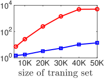
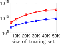
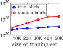
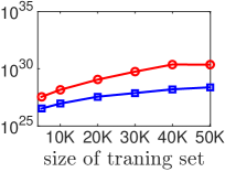
Figure 1: Comparing different complexity measures on a VGG network trained on subsets of CIFAR10 dataset with true (blue line) or random (red line) labels. We plot norm divided by margin to avoid scaling issues (see Section 2), where for each complexity measure, we drop the terms that only depend on depth or number of hidden units; e.g. for 2subscript2\ell_{2}-path norm we plot γmargin2jk=0d[hk]i=1dWi2[ji,ji1]superscriptsubscript𝛾margin2subscript𝑗superscriptsubscriptproduct𝑘0𝑑delimited-[]subscript𝑘superscriptsubscriptproduct𝑖1𝑑superscriptsubscript𝑊𝑖2subscript𝑗𝑖subscript𝑗𝑖1\gamma_{\text{margin}}^{-2}\sum_{j\in\prod_{k=0}^{d}[h_{k}]}\prod_{i=1}^{d}W_{i}^{2}[j_{i},j_{i-1}].We also set the margin over training set S𝑆S to be 5thsuperscript5𝑡5^{th}-percentile of the margins of the data points in S𝑆S, i.e. Prc5{f𝐰(xi)[yi]maxyyif𝐰(𝐱)[y]|(xi,yi)S}subscriptPrc5conditional-setsubscript𝑓𝐰subscript𝑥𝑖delimited-[]subscript𝑦𝑖subscript𝑦subscript𝑦𝑖subscript𝑓𝐰𝐱delimited-[]𝑦subscript𝑥𝑖subscript𝑦𝑖𝑆\text{Prc}_{5}\left\{f_{\mathbf{w}}(x_{i})[y_{i}]-\max_{y\neq y_{i}}f_{\mathbf{w}}(\mathbf{x})[y]|(x_{i},y_{i})\in S\right\}. In all experiments, the training error of the learned network is zero. The plots indicate that these measures can explain the generalization as the complexity of model learned with random labels is always higher than the one learned with true labels. Furthermore, the gap between the complexity of models learned with true and random labels increases as we increase the size of the training set.

As an initial empirical investigation of the appropriateness of the different complexity measures, we compared the complexity (under each of the above measures) of models trained on true versus random labels. We would expect to see two phenomena: first, the complexity of models trained on true labels should be substantially lower than those trained on random labels, corresponding to their better generalization ability. Second, when training on random labels, we expect capacity to increase almost linearly with the number of training examples, since every extra example requires new capacity in order to fit it’s random label. However, when training on true labels we expect the model to capture the true functional dependence between input and output and thus fitting more training examples should only require small increases in the capacity of the network. The results are reported in Figure 1. We indeed observe a gap between the complexity of models learned on real and random labels for all four norms, with the difference in increase in capacity between true and random labels being most pronounced for the 2subscript2\ell_{2} norm and 2subscript2\ell_{2}-path norm.

In Section 3 we present further empirical investigations of the appropriateness of these complexity measures to explaining other phenomena.

2.3 Lipschitz Continuity and Robustness

The measures/norms we discussed so far also control the Lipschitz constant of the network with respect to its input. Is the capacity control achieved through the bound on the Lipschitz constant? Is bounding the Lipschitz constant alone enough for generalization? To answer these questions, and in order to understand capacity control in terms of Lipschitz continuity more broadly, we review here the relevant guarantees.

Given an input space 𝒳𝒳\mathcal{X} and metric \mathcal{M}, a function f:𝒳:𝑓𝒳f:\mathcal{X}\rightarrow\mathbb{R} on a metric space (𝒳,)𝒳(\mathcal{X},\mathcal{M}) is called a Lipschitz function if there exists a constant Csubscript𝐶C_{\mathcal{M}}, such that |f(x)f(y)|C(x,y)𝑓𝑥𝑓𝑦subscript𝐶𝑥𝑦\left\lvert{f(x)-f(y)}\right\rvert\leq C_{\mathcal{M}}\mathcal{M}(x,y). Luxburg and Bousquet [13] studied the capacity of functions with bounded Lipschitz constant on metric space (𝒳,)𝒳(\mathcal{X},\mathcal{M}) with a finite diameter diam(𝒳)=supx,yX(x,y)subscriptdiam𝒳subscriptsupremum𝑥𝑦𝑋𝑥𝑦\text{diam}_{\mathcal{M}}(\mathcal{X})=\sup_{x,y\in X}\mathcal{M}(x,y) and showed that the capacity is proportional to (Cγmargin)ndiam(𝒳)superscriptsubscript𝐶subscript𝛾margin𝑛subscriptdiam𝒳\left(\frac{C_{\mathcal{M}}}{\gamma_{\text{margin}}}\right)^{n}\text{diam}_{\mathcal{M}}(\mathcal{X}). This capacity bound is weak as it has an exponential dependence on input size.

Another related approach is through algorithmic robustness as suggested by Xu and Mannor [28]. Given ϵ>0italic-ϵ0\epsilon>0, the model f𝐰subscript𝑓𝐰f_{\mathbf{w}} found by a learning algorithm is K𝐾K robust if 𝒳𝒳\mathcal{X} can be partitioned into K𝐾K disjoint sets, denoted as {Ci}i=1Ksuperscriptsubscriptsubscript𝐶𝑖𝑖1𝐾\{C_{i}\}_{i=1}^{K}, such that for any pair (𝐱,y)𝐱𝑦(\mathbf{x},y) in the training set 𝐬𝐬\mathbf{s} ,333Xu and Mannor [28] have defined the robustness as a property of learning algorithm given the model class and the training set. Here since we are focused on the learned model, we introduce it as a property of the model.

𝐱,𝐳Ci|(𝐰,𝐱)(𝐰,𝐳)|ϵ𝐱𝐳subscript𝐶𝑖𝐰𝐱𝐰𝐳italic-ϵ\mathbf{x},\mathbf{z}\in C_{i}\Rightarrow\left\lvert{\ell(\mathbf{w},\mathbf{x})-\ell(\mathbf{w},\mathbf{z})}\right\rvert\leq\epsilon (3)

Xu and Mannor [28] showed the capacity of a model class whose models are K𝐾K-robust scales as K𝐾K. For the model class of functions with bounded Lipschitz C.C_{\left\lVert{.}\right\rVert}, K𝐾K is proportional to C.γmargin{\frac{C_{\left\lVert{.}\right\rVert}}{\gamma_{\text{margin}}}}-covering number of the input domain 𝒳𝒳\mathcal{X} under norm .\left\lVert{.}\right\rVert. However, the covering number of the input domain can be exponential in the input dimension and the capacity can still grow as (C.γmargin)n\left(\frac{C_{\left\lVert{.}\right\rVert}}{\gamma_{\text{margin}}}\right)^{n} 444Similar to margin-based bounds, we drop the term that depends on the diameter of the input space..

Returning to our original question, the Csubscript𝐶subscriptC_{\ell_{\infty}} and C2subscript𝐶subscript2C_{\ell_{2}} Lipschitz constants of the network can be bounded by i=1dWi1,superscriptsubscriptproduct𝑖1𝑑subscriptdelimited-∥∥subscript𝑊𝑖1\prod_{i=1}^{d}\left\lVert{W_{i}}\right\rVert_{1,\infty} (hence 1subscript1\ell_{1}-path norm) and i=1dWi2superscriptsubscriptproduct𝑖1𝑑subscriptdelimited-∥∥subscript𝑊𝑖2\prod_{i=1}^{d}\left\lVert{W_{i}}\right\rVert_{2}, respectively [28, 25]. This will result in a very large capacity bound that scales as (i=1dWi2γmargin)nsuperscriptsuperscriptsubscriptproduct𝑖1𝑑subscriptdelimited-∥∥subscript𝑊𝑖2subscript𝛾margin𝑛\left(\frac{\prod_{i=1}^{d}\left\lVert{W_{i}}\right\rVert_{2}}{\gamma_{\text{margin}}}\right)^{n}, which is exponential in both the input dimension and depth of the network. This shows that simply bounding the Lipschitz constant of the network is not enough to get a reasonable capacity control, and the capacity bounds of the previous Section are not merely a consequence of bounding the Lipschitz constant.

2.4 Sharpness

The notion of sharpness as a generalization measure was recently suggested by Keskar et al. [11] and corresponds to robustness to adversarial perturbations on the parameter space:

ζα(𝐰)=max|𝝂i|α(|𝐰i|+𝟏)L^(f𝐰+𝝂)L^(f𝐰)1+L^(f𝐰)max|𝝂i|α(|𝐰i|+𝟏)L^(f𝐰+𝝂)L^(f𝐰),subscript𝜁𝛼𝐰subscriptsubscript𝝂𝑖𝛼subscript𝐰𝑖1^𝐿subscript𝑓𝐰𝝂^𝐿subscript𝑓𝐰1^𝐿subscript𝑓𝐰similar-to-or-equalssubscriptsubscript𝝂𝑖𝛼subscript𝐰𝑖1^𝐿subscript𝑓𝐰𝝂^𝐿subscript𝑓𝐰\zeta_{\alpha}(\mathbf{w})=\frac{\max_{\left\lvert{\bm{\nu}_{i}}\right\rvert\leq\alpha(\left\lvert{\mathbf{w}_{i}}\right\rvert+\mathbf{1})}\widehat{L}(f_{\mathbf{w}+\bm{\nu}})-\widehat{L}(f_{\mathbf{w}})}{1+\widehat{L}(f_{\mathbf{w}})}\simeq\max_{\left\lvert{\bm{\nu}_{i}}\right\rvert\leq\alpha(\left\lvert{\mathbf{w}_{i}}\right\rvert+\mathbf{1})}\widehat{L}(f_{\mathbf{w}+\bm{\nu}})-\widehat{L}(f_{\mathbf{w}}), (4)

where the training error L^(f𝐰)^𝐿subscript𝑓𝐰\widehat{L}(f_{\mathbf{w}}) is generally very small in the case of neural networks in practice, so we can simply drop it from the denominator without a significant change in the sharpness value.

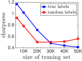
As we will explain below, sharpness defined this way does not capture the generalization behavior. To see this, we first examine whether sharpness can predict the generalization behavior for networks trained on true vs random labels. In the left plot of Figure 2, we plot the sharpness for networks trained on true vs random labels. While sharpness correctly predicts the generalization behavior for bigger networks, for networks of smaller size, those trained on random labels have less sharpness than the ones trained on true labels. Furthermore sharpness defined above depends on the scale of 𝐰𝐰\mathbf{w} and can be artificially increased or decreased by changing the scale of the parameters. Therefore, sharpness alone is not sufficient to control the capacity of the network.

Instead, we advocate viewing a related notion of expected sharpness in the context of the PAC-Bayesian framework. Viewed this way, it becomes clear that sharpness controls only one of two relevant terms, and must be balanced with some other measure such as norm. Together, sharpness and norm do provide capacity control and can explain many of the observed phenomena. This connection between sharpness and the PAC-Bayes framework was also recently noted by Dziugaite and Roy [7].

The PAC-Bayesian framework [15, 16] provides guarantees on the expected error of a randomized predictor (hypothesis), drawn form a distribution denoted 𝒬𝒬\mathcal{Q} and sometimes referred to as a “posterior” (although it need not be the Bayesian posterior), that depends on the training data. Let f𝐰subscript𝑓𝐰f_{\mathbf{w}} be any predictor (not necessarily a neural network) learned from training data. We consider a distribution 𝒬𝒬\mathcal{Q} over predictors with weights of the form 𝐰+𝝂𝐰𝝂\mathbf{w}+\bm{\nu}, where 𝐰𝐰\mathbf{w} is a single predictor learned from the training set, and 𝝂𝝂\bm{\nu} is a random variable. Then, given a “prior” distribution P𝑃P over the hypothesis that is independent of the training data, with probability at least 1δ1𝛿1-\delta over the draw of the training data, the expected error of f𝐰+𝝂subscript𝑓𝐰𝝂f_{\mathbf{w}+\bm{\nu}} can be bounded as follows [14]:

𝔼𝝂[L(f𝐰+𝝂)]𝔼𝝂[L^(f𝐰+𝝂)]+𝔼𝝂[L^(f𝐰+𝝂)]𝒦+𝒦subscript𝔼𝝂delimited-[]𝐿subscript𝑓𝐰𝝂subscript𝔼𝝂delimited-[]^𝐿subscript𝑓𝐰𝝂subscript𝔼𝝂delimited-[]^𝐿subscript𝑓𝐰𝝂𝒦𝒦\mathbb{E}_{\bm{\nu}}[L(f_{\mathbf{w}+\bm{\nu}})]\leq\mathbb{E}_{\bm{\nu}}[\widehat{L}(f_{\mathbf{w}+\bm{\nu}})]+\sqrt{\mathbb{E}_{\bm{\nu}}[\widehat{L}(f_{\mathbf{w}+\bm{\nu}})]\mathcal{K}}+\mathcal{K} (5)

where 𝒦=2(KL(𝐰+𝝂P)+ln2mδ)m1𝒦2𝐾𝐿𝐰conditional𝝂𝑃2𝑚𝛿𝑚1\mathcal{K}=\frac{2\left(KL\left(\mathbf{w}+\bm{\nu}\|P\right)+\ln\frac{2m}{\delta}\right)}{m-1}. When the training loss 𝔼𝝂[L^(f𝐰+𝝂)]subscript𝔼𝝂delimited-[]^𝐿subscript𝑓𝐰𝝂\mathbb{E}_{\bm{\nu}}[\widehat{L}(f_{\mathbf{w}+\bm{\nu}})] is smaller than 𝒦𝒦\mathcal{K}, then the last term dominates. This is often the case for neural networks with small enough perturbation. One can also get the the following weaker bound:

𝔼𝝂[L(f𝐰+𝝂)]𝔼𝝂[L^(f𝐰+𝝂)]+4(KL(𝐰+𝝂P)+ln2mδ)msubscript𝔼𝝂delimited-[]𝐿subscript𝑓𝐰𝝂subscript𝔼𝝂delimited-[]^𝐿subscript𝑓𝐰𝝂4𝐾𝐿𝐰conditional𝝂𝑃2𝑚𝛿𝑚\mathbb{E}_{\bm{\nu}}[L(f_{\mathbf{w}+\bm{\nu}})]\leq\mathbb{E}_{\bm{\nu}}[\widehat{L}(f_{\mathbf{w}+\bm{\nu}})]+4\sqrt{\frac{\left(KL\left(\mathbf{w}+\bm{\nu}\|P\right)+\ln\frac{2m}{\delta}\right)}{m}} (6)

The above inequality clearly holds for 𝒦1𝒦1\mathcal{K}\geq 1 and for 𝒦<1𝒦1\mathcal{K}<1 it can be derived from Equation (5) by upper bounding the loss in the second term by 111. We can rewrite the above bound as follows:

𝔼𝝂[L(f𝐰+𝝂)]L^(f𝐰)+𝔼𝝂[L^(f𝐰+𝝂)]L^(f𝐰)expected sharpness+41m(KL(𝐰+𝝂P)+ln2mδ)subscript𝔼𝝂delimited-[]𝐿subscript𝑓𝐰𝝂^𝐿subscript𝑓𝐰subscriptsubscript𝔼𝝂delimited-[]^𝐿subscript𝑓𝐰𝝂^𝐿subscript𝑓𝐰expected sharpness41𝑚𝐾𝐿𝐰conditional𝝂𝑃2𝑚𝛿\mathbb{E}_{\bm{\nu}}[L(f_{\mathbf{w}+\bm{\nu}})]\leq\widehat{L}(f_{\mathbf{w}})+\underbrace{\mathbb{E}_{\bm{\nu}}[\widehat{L}(f_{\mathbf{w}+\bm{\nu}})]-\widehat{L}(f_{\mathbf{w}})}_{\text{expected sharpness}}+4\sqrt{\frac{1}{m}\left(KL\left(\mathbf{w}+\bm{\nu}\|P\right)+\ln\frac{2m}{\delta}\right)} (7)
Refer to caption
Refer to caption
Refer to caption
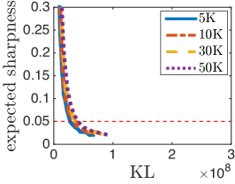
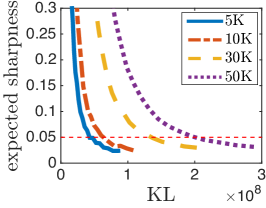
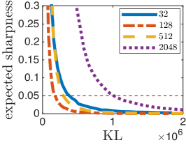
Figure 2: Sharpness and PAC-Bayes measures on a VGG network trained on subsets of CIFAR10 dataset with true or random labels. In the left panel, we plot max sharpness, which we calculate as suggested by Keskar et al. [11] where the perturbation for parameter wisubscript𝑤𝑖w_{i} has magnitude 5.104(|wi|+1)superscript5.104subscript𝑤𝑖15.10^{-4}(\left\lvert{w_{i}}\right\rvert+1). The middle and right plots demonstrate the relationship between expected sharpness and KL divergence in PAC-Bayes analysis for true and random labels respectively. For PAC-Bayes plots, each point in the plot correspond to a choice of variable α𝛼\alpha where the standard deviation of the perturbation for the parameter i𝑖i is α(10|wi|+1)𝛼10subscript𝑤𝑖1\alpha(10\left\lvert{w_{i}}\right\rvert+1). The corresponding KL𝐾𝐿KL to each α𝛼\alpha is nothing but weighted 2subscript2\ell_{2} norm where the weight for each parameter is the inverse of the standard deviation of the perturbation.
true labelsrandom labels

As we can see, the PAC-Bayes bound depends on two quantities - i) the expected sharpness and ii) the Kullback Leibler (KL) divergence to the “prior” P𝑃P. The bound is valid for any distribution measure P𝑃P, any perturbation distribution 𝝂𝝂\bm{\nu} and any method of choosing 𝐰𝐰\mathbf{w} dependent on the training set. A simple way to instantiate the bound is to set P𝑃P to be a zero mean, σ2superscript𝜎2\sigma^{2} variance Gaussian distribution. Choosing the perturbation 𝝂𝝂\bm{\nu} to also be a zero mean spherical Gaussian with variance σ2superscript𝜎2\sigma^{2} in every direction, yields the following guarantee (w.p. 1δ1𝛿1-\delta over the training set):

𝔼𝝂𝒩(0,σ)n[L(f𝐰+𝝂)]L^(f𝐰)+𝔼𝝂𝒩(0,σ)n[L^(f𝐰+𝝂)]L^(f𝐰)expected sharpness+41m(𝐰222σ2KL+ln2mδ),subscript𝔼similar-to𝝂𝒩superscript0𝜎𝑛delimited-[]𝐿subscript𝑓𝐰𝝂^𝐿subscript𝑓𝐰subscriptsubscript𝔼similar-to𝝂𝒩superscript0𝜎𝑛delimited-[]^𝐿subscript𝑓𝐰𝝂^𝐿subscript𝑓𝐰expected sharpness41𝑚subscriptsuperscriptsubscriptnorm𝐰222superscript𝜎2KL2𝑚𝛿\mathbb{E}_{\bm{\nu}\sim\mathcal{N}(0,\sigma)^{n}}[L(f_{\mathbf{w}+\bm{\nu}})]\leq\widehat{L}(f_{\mathbf{w}})+\underbrace{\mathbb{E}_{\bm{\nu}\sim\mathcal{N}(0,\sigma)^{n}}[\widehat{L}(f_{\mathbf{w}+\bm{\nu}})]-\widehat{L}(f_{\mathbf{w}})}_{\text{expected sharpness}}+4\sqrt{\frac{1}{m}\bigg{(}\underbrace{\frac{\|\mathbf{w}\|_{2}^{2}}{2\sigma^{2}}}_{\text{KL}}+\ln\frac{2m}{\delta}\bigg{)}}, (8)

Another interesting approach is to set the variance of the perturbation to each parameter with respect to the magnitude of the parameter. For example if σi=α|wi|+βsubscript𝜎𝑖𝛼subscript𝑤𝑖𝛽\sigma_{i}=\alpha\left\lvert{w_{i}}\right\rvert+\beta, then the KL term in the above expression changes to iwi22σi2subscript𝑖superscriptsubscript𝑤𝑖22superscriptsubscript𝜎𝑖2\sum_{i}\frac{w_{i}^{2}}{2\sigma_{i}^{2}}.

The above generalization guarantees give a clear way to think about capacity control jointly in terms of both the expected sharpness and the norm, and as we discussed earlier indicates that sharpness by itself cannot control the capacity without considering the scaling. In the above generalization bound, norms and sharpness interact in a direct way depending on σ𝜎\sigma, as increasing the norm by decreasing σ𝜎\sigma causes decrease in sharpness and vice versa. It is therefore important to find the right balance between the norm and sharpness by choosing σ𝜎\sigma appropriately in order to get a reasonable bound on the capacity.

In our experiments we observe that looking at both these measures jointly indeed makes a better predictor for the generalization error. As discussed earlier, Dziugaite and Roy [7] numerically optimize the overall PAC-Bayes generalization bound over a family of multivariate Gaussian distributions (different choices of perturbations and priors). Since the precise way the sharpness and KL-divergence are combined is not tight, certainly not in (8), nor in the more refined bound used by Dziugaite and Roy [7], we prefer shying away from numerically optimizing the balance between sharpness and the KL-divergence. Instead, we propose using bi-criteria plots, where sharpness and KL-divergence are plotted against each other, as we vary the perturbation variance. For example, in the center and right panels of Figure 2 we show such plots for networks trained on true and random labels respectively. We see that although sharpness by itself is not sufficient for explaining generalization in this setting (as we saw in the left panel), the bi-criteria plots are significantly lower for the true labels. Even more so, the change in the bi-criteria plot as we increase the number of samples is significantly larger with random labels, correctly capturing the required increase in capacity. For example, to get a fixed value of expected sharpness such as ϵ=0.05italic-ϵ0.05\epsilon=0.05, networks trained with random labels require higher norm compared to those trained with true labels. This behavior is in agreement with our earlier discussion, that sharpness is sensitive to scaling of the parameters and is not a capacity control measure as it can be artificially changed by scaling the network. However, combined with the norm, sharpness does seem to provide a capacity measure.

3 Empirical Investigation

In this section we investigate the ability of the discussed measures to explain the the generalization phenomenon discussed in the Introduction. We already saw in Figures 1 and 2 that these measures capture the difference in generalization behavior of models trained on true or random labels, including the increase in capacity as the sample size increases, and the difference in this increase between true and random labels.

Different Global Minima

Given different global minima of the training loss on the same training set and with the same model class, can these measures indicate which model is going to generalize better? In order to verify this property, we can calculate each measure on several different global minima and see if lower values of the measure imply lower generalization error. In order to find different global minima for the training loss, we design an experiment where we force the optimization methods to converge to different global minima with varying generalization abilities by forming a confusion set that includes samples with random labels. The optimization is done on the loss that includes examples from both the confusion set and the training set. Since deep learning models have very high capacity, the optimization over the union of confusion set and training set generally leads to a point with zero error over both confusion and training sets which thus is a global minima for the training set.

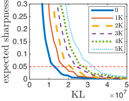
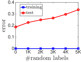
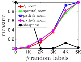
We randomly select a subset of CIFAR10 dataset with 10000 data points as the training set and our goal is to find networks that have zero error on this set but different generalization abilities on the test set. In order to do that, we train networks on the union of the training set with fixed size 10000 and confusion sets with varying sizes that consists of CIFAR10 samples with random labels; and we evaluate the learned model on an independent test set. The trained network achieves zero training error but as shown in Figure 3, the test error of the model increases with increasing size of the confusion set. The middle panel of this Figure suggests that the norm of the learned networks can indeed be predictive of their generalization behavior. However, we again observe that sharpness has a poor behavior in these experiments. The right panel of this figure also suggests that PAC-Bayes measure of joint sharpness and KL divergence, has better behavior - for a fixed expected sharpness, networks that have higher generalization error, have higher norms.

Increasing Network Size

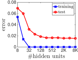
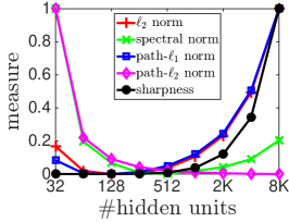
We also repeat the experiments conducted by Neyshabur et al. [19] where a fully connected feedforward network is trained on MNIST dataset with varying number of hidden units and we check the values of different complexity measures on each of the learned networks.The left panel in Figure 4 shows the training and test error for this experiment. While 32 hidden units are enough to fit the training data, we observe that networks with more hidden units generalize better. Since the optimization is done without any explicit regularization, the only possible explanation for this phenomenon is the implicit regularization by the optimization algorithm. Therefore, we expect a sensible complexity measure to decrease beyond 32 hidden units and behave similar to the test error. Different measures are reported for learned networks. The middle panel suggest that all margin/norm based complexity measures decrease for larger networks up to 128 hidden units. For networks with more hidden units, 2subscript2\ell_{2} norm and 1subscript1\ell_{1}-path norm increase with the size of the network. The middle panel suggest that 2subscript2\ell_{2}-path norm can provide some explanation for this phenomenon. However, as we discussed in Section 2, the actual complexity measure based on 2subscript2\ell_{2}-path norm also depends on the number of hidden units and taking this into account indicates that the measure based on 2subscript2\ell_{2}-path norm cannot explain this phenomenon. This is also the case for the margin based measure that depends on the spectral norm. In subsection 2.3 we discussed another complexity measure that also depends the spectral norm through Lipschitz continuity or robustness argument. Even though this bound is very loose, it is monotonic with respect to the spectral norm that is reported in the plots. Unfortunately, we do observe some increase in spectral norm by increasing number of hidden units beyond 512. The right panel shows that the joint PAC-Bayes measure decrease for larger networks up to size 128 but fails to explain this generalization behavior for larger networks. This suggests that the measures looked so far are not sufficient to explain all the generalization phenomenon observed in neural networks.
Refer to caption
Refer to caption
Refer to caption
Figure 3: Experiments on global minima with poor generalization. For each experiment, a VGG network is trained on union of a subset of CIFAR10 dataset with size 10000 containing samples with true labels and another subset of CIFAR10 datasets with varying size containing random labels. The learned networks are all global minima for the objective function on the subset with true labels. The left plot indicates the training and test errors based on the size of the set with random labels. The plot in the middle shows change in different measures based on the size of the set with random labels. The plot on the right indicates the relationship between expected sharpness and KL in PAC-bayes for each of the experiments. Measures are calculated as explained in Figures 1 and 2.
Refer to caption
Refer to caption
Refer to caption
Figure 4: The generalization of two layer perceptron trained on MNIST dataset with varying number of hidden units. The left plot indicates the training and test errors. The test error decreases as the size increases. The middle plot shows different measures for each of the trained networks. The plot on the right indicates the relationship between expected sharpness and KL in PAC-Bayes for each of the experiments. Measures are calculated as explained in Figures 1 and 2.

4 Bounding Sharpness

So far we have discussed margin based and sharpness based complexity measures to understand capacity. We have also discussed how sharpness based complexity measures in combination with norms characterize the generalization behavior under the PAC-Bayes framework. In this section we study the question of what affects the sharpness of neural networks? For the case of linear predictors, sharpness only depends on the norm of the predictor. In contrast, for multilayered networks, interaction between the layers plays a major role and consequently two different networks with the same norm can have drastically different sharpness values. For example, consider a network where some subset of the layers despite having non-zero norm interact weakly with their neighbors, or are almost orthogonal to each other. Such a network will have very high sharpness value compared to a network where the neighboring layers interact strongly.

In this section we establish sufficient conditions to bound the expected sharpness of a feedforward network with ReLU activations. Such conditions serve as a useful guideline in studying what helps an optimization method to converge to less sharp optima. Unlike existing generalization bounds [4, 18, 13, 28, 25], our sharpness based bound does not suffer from exponential dependence on depth.

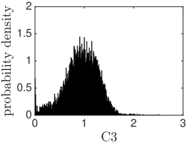
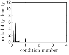
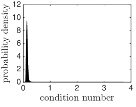
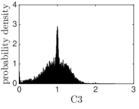
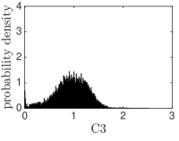
Now we discuss the conditions that affect the sharpness of a network. As discussed earlier, weak interactions between layers can cause the network to have high sharpness value. Condition C1𝐶1C1 below prevents such weak interactions (cancellations). A network can also have high sharpness if the changes in the number of activations is exponential in the perturbations to its weights, even for small perturbations. Condition C2𝐶2C2 avoids such extreme situations on activations. Finally, if a non-active node with large weights becomes active because of the perturbations in lower layers, that can lead to huge changes to the output of the network. Condition C3𝐶3C3 prevents having such spiky (in magnitude) hidden units. This leads us to the following three conditions, that help in avoiding such pathological cases.

  • (C1)::𝐶1absent(C1):

    Given x𝑥x, let x=W0𝑥subscript𝑊0x=W_{0} and D0=Isubscript𝐷0𝐼D_{0}=I. Then, for all 0a<c<bd,(Πi=abDiWi)FμhcΠi=c+1bDiWiF(Πi=acDiWi)Fformulae-sequence0𝑎𝑐𝑏𝑑subscriptnormsuperscriptsubscriptΠ𝑖𝑎𝑏subscript𝐷𝑖subscript𝑊𝑖𝐹𝜇subscript𝑐subscriptnormsuperscriptsubscriptΠ𝑖𝑐1𝑏subscript𝐷𝑖subscript𝑊𝑖𝐹subscriptnormsuperscriptsubscriptΠ𝑖𝑎𝑐subscript𝐷𝑖subscript𝑊𝑖𝐹0\leq a<c<b\leq d,\|\left(\Pi_{i=a}^{b}D_{i}W_{i}\right)\|_{F}\geq\frac{\mu}{\sqrt{h_{c}}}\|\Pi_{i=c+1}^{b}D_{i}W_{i}\|_{F}\|\left(\Pi_{i=a}^{c}D_{i}W_{i}\right)\|_{F}.

  • (C2)::𝐶2absent(C2):

    Given x𝑥x, for any level k𝑘k, 1hki[hk]1Wk,iΠj=1k1DjWjxδC2δ1subscript𝑘subscript𝑖delimited-[]subscript𝑘subscript1subscript𝑊𝑘𝑖superscriptsubscriptΠ𝑗1𝑘1subscript𝐷𝑗subscript𝑊𝑗𝑥𝛿subscript𝐶2𝛿\frac{1}{h_{k}}\sum_{i\in[h_{k}]}1_{W_{k,i}\Pi_{j=1}^{k-1}D_{j}W_{j}x\leq\delta}\leq C_{2}\delta.

  • (C3)::𝐶3absent(C3):

    For all i𝑖i, Wi2,2hiC32DiWiF2superscriptsubscriptnormsubscript𝑊𝑖22subscript𝑖superscriptsubscript𝐶32superscriptsubscriptnormsubscript𝐷𝑖subscript𝑊𝑖𝐹2\|W_{i}\|_{2,\infty}^{2}h_{i}\leq C_{3}^{2}\|D_{i}W_{i}\|_{F}^{2}.

Here, Wk,isubscript𝑊𝑘𝑖W_{k,i} denotes the weights of the ithsuperscript𝑖𝑡i^{th} output node in layer k𝑘k. Wi2,subscriptnormsubscript𝑊𝑖2\|W_{i}\|_{2,\infty} denotes the maximum L2𝐿2L2 norm of a hidden unit in layer i𝑖i. Now we state our result on the generalization error of a ReLU network, in terms of average sharpness and its norm. Let x=1norm𝑥1\|x\|=1 and h=maxi=1dhisuperscriptsubscript𝑖1𝑑subscript𝑖h=\max_{i=1}^{d}h_{i}.

Theorem 1.

Let 𝛎isubscript𝛎𝑖\bm{\nu}_{i} be a random hi×hi1subscript𝑖subscript𝑖1h_{i}\times h_{i-1} matrix with each entry distributed according to 𝒩(0,σi2)𝒩0superscriptsubscript𝜎𝑖2\mathcal{N}(0,\sigma_{i}^{2}). Then, under the conditions C1,C2,C3𝐶1𝐶2𝐶3C1,C2,C3, with probability 1δabsent1𝛿\geq 1-\delta,

𝔼𝝂𝒩(0,σ)n[L(f𝐰+𝝂)]L^(f𝐰)O([Πi=1d(1+γi)1\displaystyle\mathbb{E}_{\bm{\nu}\sim\mathcal{N}(0,\sigma)^{n}}[L(f_{\mathbf{w}+\bm{\nu}})]-\widehat{L}(f_{\mathbf{w}})\leq O\left(\left[\Pi_{i=1}^{d}\left(1+\gamma_{i}\right)-1\right.\right.
+Πi=1d(1+γiC2C3)(Πi=1d(1+γiCδC2)1)]CLxf𝐰(x)Fm)+1m(i=1dWiF2σi2+ln2mδ).\displaystyle\left.\left.+\Pi_{i=1}^{d}\left(1+\gamma_{i}C_{2}C_{3}\right)\left(\Pi_{i=1}^{d}(1+\gamma_{i}C_{\delta}C_{2})-1\right)\right]C_{L}\sum_{x}\frac{\|f_{\mathbf{w}}(x)\|_{F}}{m}\right)+\sqrt{\frac{1}{m}\left(\sum_{i=1}^{d}\frac{\|W_{i}\|_{F}^{2}}{\sigma_{i}^{2}}+\ln\frac{2m}{\delta}\right)}.

where γi=σihihi1μ2WiFsubscript𝛾𝑖subscript𝜎𝑖subscript𝑖subscript𝑖1superscript𝜇2subscriptnormsubscript𝑊𝑖𝐹\gamma_{i}=\frac{\sigma_{i}\sqrt{h_{i}}\sqrt{h_{i-1}}}{\mu^{2}\|W_{i}\|_{F}} and Cδ=2ln(dh/δ)subscript𝐶𝛿2𝑑𝛿C_{\delta}=2\sqrt{\ln(dh/\delta)}.

To understand the above generalization error bound, consider choosing γi=σCδdsubscript𝛾𝑖𝜎subscript𝐶𝛿𝑑\gamma_{i}=\frac{\sigma}{C_{\delta}d}, and we get a bound that simplifies as follows:

𝔼𝝂𝒩(0,σ)n[L(f𝐰+𝝂)]L^(f𝐰)subscript𝔼similar-to𝝂𝒩superscript0𝜎𝑛delimited-[]𝐿subscript𝑓𝐰𝝂^𝐿subscript𝑓𝐰\displaystyle\mathbb{E}_{\bm{\nu}\sim\mathcal{N}(0,\sigma)^{n}}[L(f_{\mathbf{w}+\bm{\nu}})]-\widehat{L}(f_{\mathbf{w}}) O(σ(1+(1+σC2C3)C2)CLxf𝐰(x)Fm)absent𝑂𝜎11𝜎subscript𝐶2subscript𝐶3subscript𝐶2subscript𝐶𝐿subscript𝑥subscriptnormsubscript𝑓𝐰𝑥𝐹𝑚\displaystyle\leq O\left(\sigma\left(1+(1+\sigma C_{2}C_{3})C_{2}\right)C_{L}\frac{\sum_{x}\|f_{\mathbf{w}}(x)\|_{F}}{m}\right)
+1m(d2μ4i=1dhihi1σ2+ln2mδ)1𝑚superscript𝑑2superscript𝜇4superscriptsubscript𝑖1𝑑subscript𝑖subscript𝑖1superscript𝜎22𝑚𝛿\displaystyle\quad\quad+\sqrt{\frac{1}{m}\left(\frac{d^{2}}{\mu^{4}}\sum_{i=1}^{d}\frac{h_{i}h_{i-1}}{\sigma^{2}}+\ln\frac{2m}{\delta}\right)}

If we choose large σ𝜎\sigma, then the network will have higher expected sharpness but smaller ’norm’ and vice versa. Now one can optimize over the choice of σ𝜎\sigma to balance between the terms on the right hand side and get a better capacity bound. For any reasonable choice of σ𝜎\sigma, the generalization error above, depends only linearly on depth and does not have any exponential dependence, unlike other notions of generalization. Also the error gets worse with decreasing μ𝜇\mu and increasing C2,C3subscript𝐶2subscript𝐶3C_{2},C_{3} as the sharpness of the network increases which is in accordance with our discussion of the conditions above.
Refer to caption
Refer to caption
Refer to caption
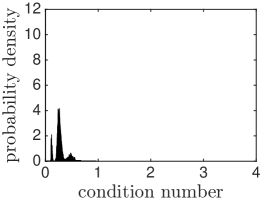
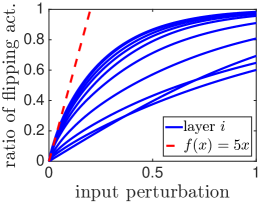
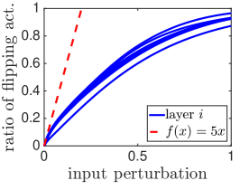
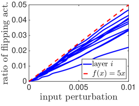
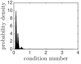
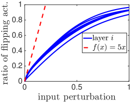
Figure 5: Verifying the conditions of Theorem 1 on a 10 layer perceptron with 1000 hidden units in each layer, i.e. more than 10,000,000 parameters on MNIST. We have numerically checked that all values are within the displayed range. Left: C1𝐶1C1: condition number of the network, i.e. 1μ1𝜇\frac{1}{\mu}. Middle: C2𝐶2C2: the ratio of activations that flip based on magnitude of perturbation. Right: C3::𝐶3absentC3: the ratio of norm of incoming weights to each hidden units with respect to average of the same quantity over hidden units in the layer.

Additionally the conditions C1C3𝐶1𝐶3C1-C3 actually hold for networks trained in practice as we verify in Figure 5, and our experiments suggest that, μ1/4,C25formulae-sequence𝜇14𝐶25\mu\geq 1/4,C2\leq 5 and C33𝐶33C3\leq 3. More details on the verification and comparing the conditions on learned network with those of random weights, are presented in the appendix.

Proof of Theorem 1

We bound the expectation as follows:

𝔼|L^(f𝐰+𝝂(x))L^(f𝐰(x))|𝔼^𝐿subscript𝑓𝐰𝝂𝑥^𝐿subscript𝑓𝐰𝑥\displaystyle\mathbb{E}\left\lvert{\widehat{L}(f_{\mathbf{w}+\bm{\nu}}(x))-\widehat{L}(f_{\mathbf{w}}(x))}\right\rvert
CL𝔼f𝐰+𝝂(x)f𝐰(x)Fabsentsubscript𝐶𝐿𝔼subscriptnormsubscript𝑓𝐰𝝂𝑥subscript𝑓𝐰𝑥𝐹\displaystyle\quad\quad\leq C_{L}\mathbb{E}\|f_{\mathbf{w}+\bm{\nu}}(x)-f_{\mathbf{w}}(x)\|_{F}
=(i)CL𝔼(W+𝝂)d(Πi=1d1D^i(W+𝝂)i)xWd(Πi=1d1DiWi)xFsuperscript𝑖absentsubscript𝐶𝐿𝔼subscriptnormsubscript𝑊𝝂𝑑superscriptsubscriptΠ𝑖1𝑑1subscript^𝐷𝑖subscript𝑊𝝂𝑖𝑥subscript𝑊𝑑superscriptsubscriptΠ𝑖1𝑑1subscript𝐷𝑖subscript𝑊𝑖𝑥𝐹\displaystyle\quad\quad\stackrel{{\scriptstyle(i)}}{{=}}C_{L}\mathbb{E}\|(W+\bm{\nu})_{d}\left(\Pi_{i=1}^{d-1}\widehat{D}_{i}(W+\bm{\nu})_{i}\right)*x-W_{d}\left(\Pi_{i=1}^{d-1}D_{i}W_{i}\right)*x\|_{F}
CL𝔼(W+𝝂)d(Πi=1d1Di(W+𝝂)i)xWd(Πi=1d1DiWi)xFabsentsubscript𝐶𝐿𝔼subscriptnormsubscript𝑊𝝂𝑑superscriptsubscriptΠ𝑖1𝑑1subscript𝐷𝑖subscript𝑊𝝂𝑖𝑥subscript𝑊𝑑superscriptsubscriptΠ𝑖1𝑑1subscript𝐷𝑖subscript𝑊𝑖𝑥𝐹\displaystyle\quad\quad\leq C_{L}\mathbb{E}\|(W+\bm{\nu})_{d}\left(\Pi_{i=1}^{d-1}D_{i}(W+\bm{\nu})_{i}\right)*x-W_{d}\left(\Pi_{i=1}^{d-1}D_{i}W_{i}\right)*x\|_{F}
+CL𝔼(W+𝝂)d(Πi=1d1D^i(W+𝝂)i)x(W+𝝂)d(Πi=1d1Di(W+𝝂)i)xFsubscript𝐶𝐿𝔼subscriptnormsubscript𝑊𝝂𝑑superscriptsubscriptΠ𝑖1𝑑1subscript^𝐷𝑖subscript𝑊𝝂𝑖𝑥subscript𝑊𝝂𝑑superscriptsubscriptΠ𝑖1𝑑1subscript𝐷𝑖subscript𝑊𝝂𝑖𝑥𝐹\displaystyle\quad\quad\quad\quad+C_{L}\mathbb{E}\|(W+\bm{\nu})_{d}\left(\Pi_{i=1}^{d-1}\widehat{D}_{i}(W+\bm{\nu})_{i}\right)*x-(W+\bm{\nu})_{d}\left(\Pi_{i=1}^{d-1}D_{i}(W+\bm{\nu})_{i}\right)*x\|_{F}
CL𝔼(W+𝝂)d(Πi=1d1Di(W+𝝂)i)xWd(Πi=1d1DiWi)xF+CL𝔼ErrdF,absentsubscript𝐶𝐿𝔼subscriptnormsubscript𝑊𝝂𝑑superscriptsubscriptΠ𝑖1𝑑1subscript𝐷𝑖subscript𝑊𝝂𝑖𝑥subscript𝑊𝑑superscriptsubscriptΠ𝑖1𝑑1subscript𝐷𝑖subscript𝑊𝑖𝑥𝐹subscript𝐶𝐿𝔼subscriptnorm𝐸𝑟subscript𝑟𝑑𝐹\displaystyle\quad\quad\leq C_{L}\mathbb{E}\|(W+\bm{\nu})_{d}\left(\Pi_{i=1}^{d-1}D_{i}(W+\bm{\nu})_{i}\right)*x-W_{d}\left(\Pi_{i=1}^{d-1}D_{i}W_{i}\right)*x\|_{F}+C_{L}\mathbb{E}\|Err_{d}\|_{F}, (9)

where Errd=(W+𝝂)d(Πi=1d1D^i(W+𝝂)i)x(W+𝝂)d(Πi=1d1Di(W+𝝂)i)xF𝐸𝑟subscript𝑟𝑑subscriptnormsubscript𝑊𝝂𝑑superscriptsubscriptΠ𝑖1𝑑1subscript^𝐷𝑖subscript𝑊𝝂𝑖𝑥subscript𝑊𝝂𝑑superscriptsubscriptΠ𝑖1𝑑1subscript𝐷𝑖subscript𝑊𝝂𝑖𝑥𝐹Err_{d}=\|(W+\bm{\nu})_{d}\left(\Pi_{i=1}^{d-1}\widehat{D}_{i}(W+\bm{\nu})_{i}\right)*x-(W+\bm{\nu})_{d}\left(\Pi_{i=1}^{d-1}D_{i}(W+\bm{\nu})_{i}\right)*x\|_{F}. (i)𝑖(i) D^isubscript^𝐷𝑖\widehat{D}_{i} is the diagonal matrix with 0’s and 1’s corresponding to the activation pattern of the perturbed network f𝐰+𝝂(x)subscript𝑓𝐰𝝂𝑥f_{\mathbf{w}+\bm{\nu}}(x).

The first term in the equation (9) corresponds to error due to perturbation of a network with unchanged activations (linear network). Intuitively this is small when any subset of successive layers of the network do no interact weakly with each other (not orthogonal to each other). Condition C1𝐶1C1 captures this intuition and we bound this error in Lemma 10.

Lemma 1.

Let 𝛎isubscript𝛎𝑖\bm{\nu}_{i} be a random hi×hi1subscript𝑖subscript𝑖1h_{i}\times h_{i-1} matrix with each entry distributed according to 𝒩(0,σi2)𝒩0superscriptsubscript𝜎𝑖2\mathcal{N}(0,\sigma_{i}^{2}). Then, under the condition C1𝐶1C1,

𝔼(W+𝝂)d(Πi=1d1Di(W+𝝂)i)xWd(Πi=1d1DiWi)xF(Πi=1d(1+σihihi1μ2DiWiF)1)f𝐰(x)F.𝔼subscriptdelimited-∥∥subscript𝑊𝝂𝑑superscriptsubscriptΠ𝑖1𝑑1subscript𝐷𝑖subscript𝑊𝝂𝑖𝑥subscript𝑊𝑑superscriptsubscriptΠ𝑖1𝑑1subscript𝐷𝑖subscript𝑊𝑖𝑥𝐹superscriptsubscriptΠ𝑖1𝑑1subscript𝜎𝑖subscript𝑖subscript𝑖1superscript𝜇2subscriptnormsubscript𝐷𝑖subscript𝑊𝑖𝐹1subscriptdelimited-∥∥subscript𝑓𝐰𝑥𝐹\mathbb{E}\|(W+\bm{\nu})_{d}\left(\Pi_{i=1}^{d-1}D_{i}(W+\bm{\nu})_{i}\right)*x-W_{d}\left(\Pi_{i=1}^{d-1}D_{i}W_{i}\right)*x\|_{F}\\ \leq\left(\Pi_{i=1}^{d}\left(1+\frac{\sigma_{i}\sqrt{h_{i}h_{i-1}}}{\mu^{2}\|D_{i}W_{i}\|_{F}}\right)-1\right)\|f_{\mathbf{w}}(x)\|_{F}.

The second term in the equation (9) captures the perturbation error due to change in activations. If a tiny perturbation can cause exponentially many changes in number of active nodes, then that network will have huge sharpness. Condition C2𝐶2C2 and C3𝐶3C3 essentially characterize the behavior of sensitivity of activation patterns to perturbations, leading to a bound on this term in Lemma 2.

Lemma 2.

Let 𝛎isubscript𝛎𝑖\bm{\nu}_{i} be a random hi×hi1subscript𝑖subscript𝑖1h_{i}\times h_{i-1} matrix with each entry distributed according to 𝒩(0,σi2)𝒩0superscriptsubscript𝜎𝑖2\mathcal{N}(0,\sigma_{i}^{2}). Then, under the conditions C1𝐶1C1, C2𝐶2C2 and C3𝐶3C3, with probability 1δabsent1𝛿\geq 1-\delta, for all 1kd1𝑘𝑑1\leq k\leq d,

D^kDk1O(C2hkCδσkf𝐰k1F)subscriptnormsubscript^𝐷𝑘subscript𝐷𝑘1𝑂subscript𝐶2subscript𝑘subscript𝐶𝛿subscript𝜎𝑘subscriptnormsubscriptsuperscript𝑓𝑘1𝐰𝐹\|\widehat{D}_{k}-D_{k}\|_{1}\leq O\left(C_{2}h_{k}C_{\delta}\sigma_{k}\|f^{k-1}_{\mathbf{w}}\|_{F}\right)

and

𝔼ErrkFO(Πi=1k(1+γiC2C3)(Πi=1k(1+γiCδC2)1)f𝐰kF).𝔼subscriptnorm𝐸𝑟subscript𝑟𝑘𝐹𝑂superscriptsubscriptΠ𝑖1𝑘1subscript𝛾𝑖subscript𝐶2subscript𝐶3superscriptsubscriptΠ𝑖1𝑘1subscript𝛾𝑖subscript𝐶𝛿subscript𝐶21subscriptnormsubscriptsuperscript𝑓𝑘𝐰𝐹\mathbb{E}\|Err_{k}\|_{F}\leq O\left(\Pi_{i=1}^{k}\left(1+\gamma_{i}C_{2}C_{3}\right)\left(\Pi_{i=1}^{k}(1+\gamma_{i}C_{\delta}C_{2})-1\right)\|f^{k}_{\mathbf{w}}\|_{F}\right).

where γi=σihihi1μ2DiWiFsubscript𝛾𝑖subscript𝜎𝑖subscript𝑖subscript𝑖1superscript𝜇2subscriptnormsubscript𝐷𝑖subscript𝑊𝑖𝐹\gamma_{i}=\frac{\sigma_{i}\sqrt{h_{i}}\sqrt{h_{i-1}}}{\mu^{2}\|D_{i}W_{i}\|_{F}} and Cδ=2ln(dh/δ)subscript𝐶𝛿2𝑑𝛿C_{\delta}=2\sqrt{\ln(dh/\delta)}.

Hence, from Lemma 10 and Lemma 2 we get,

𝔼|L^(f𝐰+𝝂(x))L^(f𝐰(x))|𝔼^𝐿subscript𝑓𝐰𝝂𝑥^𝐿subscript𝑓𝐰𝑥\displaystyle\mathbb{E}\left\lvert{\widehat{L}(f_{\mathbf{w}+\bm{\nu}}(x))-\widehat{L}(f_{\mathbf{w}}(x))}\right\rvert
[Πi=1d(1+γi)1+Πi=1d(1+γiC2C3)(Πi=1d(1+γiCδC2)1)]CLf𝐰(x)F.absentdelimited-[]superscriptsubscriptΠ𝑖1𝑑1subscript𝛾𝑖1superscriptsubscriptΠ𝑖1𝑑1subscript𝛾𝑖subscript𝐶2subscript𝐶3superscriptsubscriptΠ𝑖1𝑑1subscript𝛾𝑖subscript𝐶𝛿subscript𝐶21subscript𝐶𝐿subscriptnormsubscript𝑓𝐰𝑥𝐹\displaystyle\leq\left[\Pi_{i=1}^{d}\left(1+\gamma_{i}\right)-1+\Pi_{i=1}^{d}\left(1+\gamma_{i}C_{2}C_{3}\right)\left(\Pi_{i=1}^{d}(1+\gamma_{i}C_{\delta}C_{2})-1\right)\right]C_{L}\|f_{\mathbf{w}}(x)\|_{F}.

Here γi=σihihi1μ2DiWiFsubscript𝛾𝑖subscript𝜎𝑖subscript𝑖subscript𝑖1superscript𝜇2subscriptnormsubscript𝐷𝑖subscript𝑊𝑖𝐹\gamma_{i}=\frac{\sigma_{i}\sqrt{h_{i}}\sqrt{h_{i-1}}}{\mu^{2}\|D_{i}W_{i}\|_{F}}. Substituting the above bound on expected sharpness in the PAC-Bayes result (equation (7)), gives the result.

5 Conclusion

Learning with deep neural networks displays good generalization behavior in practice, a phenomenon that remains largely unexplained. In this paper we discussed different candidate complexity measures that might explain generalization in neural networks. We outline a concrete methodology for investigating such measures, and report on experiments studying how well the measures explain different phenomena. While there is no clear choice yet, some combination of expected sharpness and norms do seem to capture much of the generalization behavior of neural networks. A major issue still left unresolved is how the choice of optimization algorithm biases such complexity to be low, and what is the precise relationship between optimization and implicit regularization.

References

  • Anthony and Bartlett [2009] M. Anthony and P. L. Bartlett. Neural network learning: Theoretical foundations. cambridge university press, 2009.
  • Bartlett [1998] P. L. Bartlett. The sample complexity of pattern classification with neural networks: the size of the weights is more important than the size of the network. IEEE transactions on Information Theory, 44(2):525–536, 1998.
  • Bartlett [2017] P. L. Bartlett. The impact of the nonlinearity on the VC-dimension of a deep network. Preprint, 2017.
  • Bartlett and Mendelson [2002] P. L. Bartlett and S. Mendelson. Rademacher and gaussian complexities: Risk bounds and structural results. Journal of Machine Learning Research, 3(Nov):463–482, 2002.
  • Bartlett et al. [1998] P. L. Bartlett, V. Maiorov, and R. Meir. Almost linear vc dimension bounds for piecewise polynomial networks. Neural computation, 10(8):2159–2173, 1998.
  • Chaudhari et al. [2016] P. Chaudhari, A. Choromanska, S. Soatto, and Y. LeCun. Entropy-sgd: Biasing gradient descent into wide valleys. arXiv preprint arXiv:1611.01838, 2016.
  • Dziugaite and Roy [2017] G. K. Dziugaite and D. M. Roy. Computing nonvacuous generalization bounds for deep (stochastic) neural networks with many more parameters than training data. arXiv preprint arXiv:1703.11008, 2017.
  • Evgeniou et al. [2000] T. Evgeniou, M. Pontil, and T. Poggio. Regularization networks and support vector machines. Advances in computational mathematics, 13(1):1–50, 2000.
  • Hardt et al. [2016] M. Hardt, B. Recht, and Y. Singer. Train faster, generalize better: Stability of stochastic gradient descent. In ICML, 2016.
  • Harvey et al. [2017] N. Harvey, C. Liaw, and A. Mehrabian. Nearly-tight vc-dimension bounds for piecewise linear neural networks. arXiv preprint arXiv:1703.02930, 2017.
  • Keskar et al. [2016] N. S. Keskar, D. Mudigere, J. Nocedal, M. Smelyanskiy, and P. T. P. Tang. On large-batch training for deep learning: Generalization gap and sharp minima. arXiv preprint arXiv:1609.04836, 2016.
  • Langford and Caruana [2001] J. Langford and R. Caruana. (not) bounding the true error. In Proceedings of the 14th International Conference on Neural Information Processing Systems: Natural and Synthetic, pages 809–816. MIT Press, 2001.
  • Luxburg and Bousquet [2004] U. v. Luxburg and O. Bousquet. Distance-based classification with lipschitz functions. Journal of Machine Learning Research, 5(Jun):669–695, 2004.
  • McAllester [2003] D. McAllester. Simplified pac-bayesian margin bounds. Lecture notes in computer science, pages 203–215, 2003.
  • McAllester [1998] D. A. McAllester. Some PAC-Bayesian theorems. In Proceedings of the eleventh annual conference on Computational learning theory, pages 230–234. ACM, 1998.
  • McAllester [1999] D. A. McAllester. PAC-Bayesian model averaging. In Proceedings of the twelfth annual conference on Computational learning theory, pages 164–170. ACM, 1999.
  • Neyshabur et al. [2015a] B. Neyshabur, R. Salakhutdinov, and N. Srebro. Path-SGD: Path-normalized optimization in deep neural networks. In Advanced in Neural Information Processsing Systems (NIPS), 2015a.
  • Neyshabur et al. [2015b] B. Neyshabur, R. Tomioka, and N. Srebro. Norm-based capacity control in neural networks. In Proceeding of the 28th Conference on Learning Theory (COLT), 2015b.
  • Neyshabur et al. [2015c] B. Neyshabur, R. Tomioka, and N. Srebro. In search of the real inductive bias: On the role of implicit regularization in deep learning. Proceeding of the International Conference on Learning Representations workshop track, 2015c.
  • Neyshabur et al. [2016a] B. Neyshabur, R. Tomioka, R. Salakhutdinov, and N. Srebro. Data-dependent path normalization in neural networks. In the International Conference on Learning Representations, 2016a.
  • Neyshabur et al. [2016b] B. Neyshabur, Y. Wu, R. Salakhutdinov, and N. Srebro. Path-normalized optimization of recurrent neural networks with relu activations. Advances in Neural Information Processing Systems, 2016b.
  • Shalev-Shwartz and Ben-David [2014] S. Shalev-Shwartz and S. Ben-David. Understanding machine learning: From theory to algorithms. Cambridge university press, 2014.
  • Simonyan and Zisserman [2014] K. Simonyan and A. Zisserman. Very deep convolutional networks for large-scale image recognition. arXiv preprint arXiv:1409.1556, 2014.
  • Smola et al. [1998] A. J. Smola, B. Schölkopf, and K.-R. Müller. The connection between regularization operators and support vector kernels. Neural networks, 11(4):637–649, 1998.
  • Sokolic et al. [2016] J. Sokolic, R. Giryes, G. Sapiro, and M. R. Rodrigues. Generalization error of invariant classifiers. arXiv preprint arXiv:1610.04574, 2016.
  • Srebro and Shraibman [2005] N. Srebro and A. Shraibman. Rank, trace-norm and max-norm. In International Conference on Computational Learning Theory, pages 545–560. Springer Berlin Heidelberg, 2005.
  • Srebro et al. [2005] N. Srebro, J. Rennie, and T. S. Jaakkola. Maximum-margin matrix factorization. In Advances in neural information processing systems, pages 1329–1336, 2005.
  • Xu and Mannor [2012] H. Xu and S. Mannor. Robustness and generalization. Machine learning, 86(3):391–423, 2012.
  • Zhang et al. [2017] C. Zhang, S. Bengio, M. Hardt, B. Recht, and O. Vinyals. Understanding deep learning requires rethinking generalization. In International Conference on Learning Representations, 2017.

Appendix A Experiments Settings

In experiment with different network sizes, we train a two layer perceptron with ReLU activation and varying number of hidden units without Batch Normalization or dropout. In the rest of the experiments, we train a modified version of the VGG architecture [23] with the configuration 2×[64,3,3,1]2643312\times[64,3,3,1], 2×[128,3,3,1]21283312\times[128,3,3,1], 2×[256,3,3,1]22563312\times[256,3,3,1], 2×[512,3,3,1]25123312\times[512,3,3,1] where we add Batch Normalization before ReLU activations and apply 2×2222\times 2 max-pooling with window size 2 and dropout after each stack. Convolutional layers are followed by 4×4444\times 4 average pooling, a fully connected layer with 512 hidden units and finally a linear layer is added for prediction.

In all experiments we train the networks using stochastic gradient descent (SGD) with mini-batch size 64, fixed learning rate 0.01 and momentum 0.9 without weight decay. In all experiments where achieving zero training error is possible, we continue training until the cross-entropy loss is less than 104superscript10410^{-4}.

When calculating norms on a network with a Batch Normalization layer, we reparametrize the network to one that represents the exact same function without Batch Normalization as suggested in [20]. In all our figures we plot norm divided by margin to avoid scaling issues (see Section 2), where we set the margin over training set S𝑆S to be 5thsuperscript5𝑡5^{th}-percentile of the margins of the data points in S𝑆S, i.e. Prc5{f𝐰(xi)[yi]maxyyif𝐰(x)[y]|(xi,yi)S}.subscriptPrc5conditional-setsubscript𝑓𝐰subscript𝑥𝑖delimited-[]subscript𝑦𝑖subscript𝑦subscript𝑦𝑖subscript𝑓𝐰𝑥delimited-[]𝑦subscript𝑥𝑖subscript𝑦𝑖𝑆\text{Prc}_{5}\left\{f_{\mathbf{w}}(x_{i})[y_{i}]-\max_{y\neq y_{i}}f_{\mathbf{w}}(x)[y]|(x_{i},y_{i})\in S\right\}. We have also investigated other versions of the margin and observed similar behavior to this notion.

We calculate the sharpness, as suggested in [11] - for each parameter wisubscript𝑤𝑖w_{i} we bound the magnitude of perturbation by α(|wi|+1)𝛼subscript𝑤𝑖1\alpha(\left\lvert{w_{i}}\right\rvert+1) for α=5.104𝛼superscript5.104\alpha=5.10^{-4}. In order to compute the maximum perturbation (maximize the loss), we perform 2000 updates of stochastic gradient ascent starting from the minimum, with mini-batch size 64, fixed step size 0.01 and momentum 0.9.

To compute the expected sharpness, we perturb each parameter wisubscript𝑤𝑖w_{i} of the model with noise generated from Gaussian distribution with zero mean and standard deviation, α(10|wi|+1)𝛼10subscript𝑤𝑖1\alpha(10\left\lvert{w_{i}}\right\rvert+1). The expected sharpness is average over 1000 random perturbations each of which are averaged over a mini-batch of size 64. We compute the expected sharpness for different choices of α𝛼\alpha. For each value of α𝛼\alpha the KL divergence can be calculated as 1α2i(wi(10|wi|+1))21superscript𝛼2subscript𝑖superscriptsubscript𝑤𝑖10subscript𝑤𝑖12\frac{1}{\alpha^{2}}\sum_{i}\left(\frac{w_{i}}{(10\left\lvert{w_{i}}\right\rvert+1)}\right)^{2}.

Appendix B Proofs

B.1 Proof of Lemma 1

Proof.

Define g𝐰,𝝂,s(x)subscript𝑔𝐰𝝂𝑠𝑥g_{\mathbf{w},\bm{\nu},s}(x) as the network f𝐰subscript𝑓𝐰f_{\mathbf{w}} with weight Wisubscript𝑊𝑖W_{i} in every layer is𝑖𝑠i\in s replaced by 𝝂isubscript𝝂𝑖\bm{\nu}_{i}. Hence,

(W+𝝂)d\displaystyle\|(W+\bm{\nu})_{d} (Πi=1d1Di(W+𝝂)i)xWd(Πi=1d1DiWi)xFsuperscriptsubscriptΠ𝑖1𝑑1subscript𝐷𝑖subscript𝑊𝝂𝑖𝑥evaluated-atsubscript𝑊𝑑superscriptsubscriptΠ𝑖1𝑑1subscript𝐷𝑖subscript𝑊𝑖𝑥𝐹\displaystyle\left(\Pi_{i=1}^{d-1}D_{i}(W+\bm{\nu})_{i}\right)*x-W_{d}\left(\Pi_{i=1}^{d-1}D_{i}W_{i}\right)*x\|_{F}
ig𝐰,𝝂,{i}(x)F+i,jg𝐰,𝝂,{i,j}(x)F++f𝝂(x)Fabsentsubscriptnormsubscript𝑖subscript𝑔𝐰𝝂𝑖𝑥𝐹subscriptnormsubscript𝑖𝑗subscript𝑔𝐰𝝂𝑖𝑗𝑥𝐹subscriptnormsubscript𝑓𝝂𝑥𝐹\displaystyle\leq\|\sum_{i}g_{\mathbf{w},\bm{\nu},\{i\}}(x)\|_{F}+\|\sum_{i,j}g_{\mathbf{w},\bm{\nu},\{i,j\}}(x)\|_{F}+\cdots+\|f_{\bm{\nu}}(x)\|_{F} (10)

Base case: First we show the bound for terms with one noisy layer. Let g𝐰,𝝂,{k}(x)subscript𝑔𝐰𝝂𝑘𝑥g_{\mathbf{w},\bm{\nu},\{k\}}(x) denote f𝐰(x)subscript𝑓𝐰𝑥f_{\mathbf{w}}(x) with weights in layer k𝑘k, Wksubscript𝑊𝑘W_{k} replaced by 𝝂ksubscript𝝂𝑘\bm{\nu}_{k}. Now notice that,

𝔼g𝐰,𝝂,{k}(x)F𝔼subscriptnormsubscript𝑔𝐰𝝂𝑘𝑥𝐹\displaystyle\mathbb{E}\|g_{\mathbf{w},\bm{\nu},\{k\}}(x)\|_{F} =𝔼WdΠi=k+1d1DiWiDk𝝂k(Πi=1k1DiWi)xFabsent𝔼subscriptnormsubscript𝑊𝑑superscriptsubscriptΠ𝑖𝑘1𝑑1subscript𝐷𝑖subscript𝑊𝑖subscript𝐷𝑘subscript𝝂𝑘superscriptsubscriptΠ𝑖1𝑘1subscript𝐷𝑖subscript𝑊𝑖𝑥𝐹\displaystyle=\mathbb{E}\|W_{d}\Pi_{i=k+1}^{d-1}D_{i}W_{i}*D_{k}\bm{\nu}_{k}*\left(\Pi_{i=1}^{k-1}D_{i}W_{i}\right)*x\|_{F}
(i)σkWdΠi=k+1d1DiWiF(Πi=1k1DiWi)xF\displaystyle\stackrel{{\scriptstyle(i)}}{{\leq}}\sigma_{k}\|W_{d}\Pi_{i=k+1}^{d-1}D_{i}W_{i}\|_{F}\|\|\left(\Pi_{i=1}^{k-1}D_{i}W_{i}\right)*x\|_{F}
(ii)σkhkhk1μ2DkWkFWd(Πi=1d1DiWi)xFsuperscript𝑖𝑖absentsubscript𝜎𝑘subscript𝑘subscript𝑘1superscript𝜇2subscriptnormsubscript𝐷𝑘subscript𝑊𝑘𝐹subscriptnormsubscript𝑊𝑑superscriptsubscriptΠ𝑖1𝑑1subscript𝐷𝑖subscript𝑊𝑖𝑥𝐹\displaystyle\stackrel{{\scriptstyle(ii)}}{{\leq}}\sigma_{k}\frac{\sqrt{h_{k}h_{k-1}}}{\mu^{2}\|D_{k}W_{k}\|_{F}}\|W_{d}\left(\Pi_{i=1}^{d-1}D_{i}W_{i}\right)*x\|_{F}
=σkhkhk1μ2DkWkFf𝐰(x)F.absentsubscript𝜎𝑘subscript𝑘subscript𝑘1superscript𝜇2subscriptnormsubscript𝐷𝑘subscript𝑊𝑘𝐹subscriptnormsubscript𝑓𝐰𝑥𝐹\displaystyle=\sigma_{k}\frac{\sqrt{h_{k}h_{k-1}}}{\mu^{2}\|D_{k}W_{k}\|_{F}}\|f_{\mathbf{w}}(x)\|_{F}.

(i)𝑖(i) follows from Lemma 3. (ii)𝑖𝑖(ii) follows from condition C1𝐶1C1.

Induction step: Let for any set s[d],|s|=kformulae-sequence𝑠delimited-[]𝑑𝑠𝑘s\subset[d],|s|=k, the following holds:

𝔼g𝐰,𝝂,s(x)Ff𝐰(x)FΠisσihihi1μ2DiWiF.𝔼subscriptnormsubscript𝑔𝐰𝝂𝑠𝑥𝐹subscriptnormsubscript𝑓𝐰𝑥𝐹subscriptΠ𝑖𝑠subscript𝜎𝑖subscript𝑖subscript𝑖1superscript𝜇2subscriptnormsubscript𝐷𝑖subscript𝑊𝑖𝐹\mathbb{E}\|g_{\mathbf{w},\bm{\nu},s}(x)\|_{F}\leq\|f_{\mathbf{w}}(x)\|_{F}\Pi_{i\in s}\sigma_{i}\frac{\sqrt{h_{i}h_{i-1}}}{\mu^{2}\|D_{i}W_{i}\|_{F}}.

We will prove this now for terms with k+1𝑘1k+1 noisy layers.

𝔼g𝐰,𝝂,s{j},x)F\displaystyle\mathbb{E}\|g_{\mathbf{w},\bm{\nu},s\cup\{j\}},x)\|_{F} σjhjhj1μ2DjWj𝔼g𝐰,𝝂,s(x)Fabsentsubscript𝜎𝑗subscript𝑗subscript𝑗1superscript𝜇2normsubscript𝐷𝑗subscript𝑊𝑗𝔼subscriptnormsubscript𝑔𝐰𝝂𝑠𝑥𝐹\displaystyle\leq\sigma_{j}\frac{\sqrt{h_{j}h_{j-1}}}{\mu^{2}\|D_{j}W_{j}\|}\mathbb{E}\|g_{\mathbf{w},\bm{\nu},s}(x)\|_{F}
σjhjhj1μ2DjWjf𝐰(x)FΠisσihihi1μ2DiWiFabsentsubscript𝜎𝑗subscript𝑗subscript𝑗1superscript𝜇2normsubscript𝐷𝑗subscript𝑊𝑗subscriptnormsubscript𝑓𝐰𝑥𝐹subscriptΠ𝑖𝑠subscript𝜎𝑖subscript𝑖subscript𝑖1superscript𝜇2subscriptnormsubscript𝐷𝑖subscript𝑊𝑖𝐹\displaystyle\leq\sigma_{j}\frac{\sqrt{h_{j}h_{j-1}}}{\mu^{2}\|D_{j}W_{j}\|}\|f_{\mathbf{w}}(x)\|_{F}\Pi_{i\in s}\sigma_{i}\frac{\sqrt{h_{i}h_{i-1}}}{\mu^{2}\|D_{i}W_{i}\|_{F}}
=f𝐰(x)FΠis{j}σihihi1μ2DiWiFabsentsubscriptnormsubscript𝑓𝐰𝑥𝐹subscriptΠ𝑖𝑠𝑗subscript𝜎𝑖subscript𝑖subscript𝑖1superscript𝜇2subscriptnormsubscript𝐷𝑖subscript𝑊𝑖𝐹\displaystyle=\|f_{\mathbf{w}}(x)\|_{F}\Pi_{i\in s\cup\{j\}}\sigma_{i}\frac{\sqrt{h_{i}h_{i-1}}}{\mu^{2}\|D_{i}W_{i}\|_{F}}

Substituting the above expression in equation (10) gives,

(W+𝝂)d(Πi=1d1Di(W+𝝂)i)xWd(Πi=1d1DiWi)xF(Πi=1d(1+σihihi1μ2DiWiF)1)f𝐰(x)F.subscriptdelimited-∥∥subscript𝑊𝝂𝑑superscriptsubscriptΠ𝑖1𝑑1subscript𝐷𝑖subscript𝑊𝝂𝑖𝑥subscript𝑊𝑑superscriptsubscriptΠ𝑖1𝑑1subscript𝐷𝑖subscript𝑊𝑖𝑥𝐹superscriptsubscriptΠ𝑖1𝑑1subscript𝜎𝑖subscript𝑖subscript𝑖1superscript𝜇2subscriptnormsubscript𝐷𝑖subscript𝑊𝑖𝐹1subscriptdelimited-∥∥subscript𝑓𝐰𝑥𝐹\|(W+\bm{\nu})_{d}\left(\Pi_{i=1}^{d-1}D_{i}(W+\bm{\nu})_{i}\right)*x-W_{d}\left(\Pi_{i=1}^{d-1}D_{i}W_{i}\right)*x\|_{F}\\ \leq\left(\Pi_{i=1}^{d}\left(1+\frac{\sigma_{i}\sqrt{h_{i}h_{i-1}}}{\mu^{2}\|D_{i}W_{i}\|_{F}}\right)-1\right)\|f_{\mathbf{w}}(x)\|_{F}.

B.2 Proof of Lemma 2

Proof.

We prove this lemma by induction on k𝑘k. Recall that D^isubscript^𝐷𝑖\widehat{D}_{i} is the diagonal matrix with 0’s and 1’s corresponding to the activation pattern of the perturbed network f𝐰+𝝂(x)subscript𝑓𝐰𝝂𝑥f_{\mathbf{w}+\bm{\nu}}(x). Let Cδ=2ln(dh/δ)subscript𝐶𝛿2𝑑𝛿C_{\delta}=2\sqrt{\ln(dh/\delta)} and 1Esubscript1𝐸1_{E} denote the indicator function, that is 111 if the event E𝐸E is true, 00 else. We also use f𝐰k(x)superscriptsubscript𝑓𝐰𝑘𝑥f_{\mathbf{w}}^{k}(x) to denote the network truncated to level k𝑘k, in particular f𝐰k(x)=Πi=1kDkWkxsuperscriptsubscript𝑓𝐰𝑘𝑥superscriptsubscriptΠ𝑖1𝑘subscript𝐷𝑘subscript𝑊𝑘𝑥f_{\mathbf{w}}^{k}(x)=\Pi_{i=1}^{k}D_{k}W_{k}x.

Base case:

D^1D11=i1(W+𝝂)1,i,xW1,i,x<0=i1(𝐰)1,i,x2<(𝝂)1,i,x(𝐰)1,i,xi1|(𝐰)1,i,x|<|(𝝂)1,i,x|.subscriptdelimited-∥∥subscript^𝐷1subscript𝐷11subscript𝑖subscript1subscript𝑊𝝂1𝑖𝑥subscript𝑊1𝑖𝑥0subscript𝑖subscript1superscriptsubscript𝐰1𝑖𝑥2subscript𝝂1𝑖𝑥subscript𝐰1𝑖𝑥subscript𝑖subscript1subscript𝐰1𝑖𝑥subscript𝝂1𝑖𝑥\|\widehat{D}_{1}-D_{1}\|_{1}=\sum_{i}1_{\left\langle(W+\bm{\nu})_{1,i},x\right\rangle*\left\langle W_{1,i},x\right\rangle<0}=\sum_{i}1_{\left\langle(\mathbf{w})_{1,i},x\right\rangle^{2}<-\left\langle(\bm{\nu})_{1,i},x\right\rangle*\left\langle(\mathbf{w})_{1,i},x\right\rangle}\\ \leq\sum_{i}1_{\left\lvert{\left\langle(\mathbf{w})_{1,i},x\right\rangle}\right\rvert<\left\lvert{\left\langle(\bm{\nu})_{1,i},x\right\rangle}\right\rvert}.

Since 𝝂1subscript𝝂1\bm{\nu}_{1} is a random Gaussian matrix, and x1norm𝑥1\|x\|\leq 1, for any i𝑖i, |(𝝂)1,i,x|2σ1ln(dh/δ)=σ1Cδsubscript𝝂1𝑖𝑥2subscript𝜎1𝑑𝛿subscript𝜎1subscript𝐶𝛿\left\lvert{\left\langle(\bm{\nu})_{1,i},x\right\rangle}\right\rvert\leq 2\sigma_{1}\sqrt{\ln(dh/\delta)}=\sigma_{1}C_{\delta} with probability greater than 1δd1𝛿𝑑1-\frac{\delta}{d}. Hence, with probability 1δdabsent1𝛿𝑑\geq 1-\frac{\delta}{d},

D^1D11i1|(𝐰)1,i,x|σ1CδC2h1σ1Cδ.subscriptnormsubscript^𝐷1subscript𝐷11subscript𝑖subscript1subscript𝐰1𝑖𝑥subscript𝜎1subscript𝐶𝛿subscript𝐶2subscript1subscript𝜎1subscript𝐶𝛿\displaystyle\|\widehat{D}_{1}-D_{1}\|_{1}\leq\sum_{i}1_{\left\lvert{\left\langle(\mathbf{w})_{1,i},x\right\rangle}\right\rvert\leq\sigma_{1}C_{\delta}}\leq C_{2}h_{1}\sigma_{1}C_{\delta}.

This completes the base case for k=1𝑘1k=1. D^1subscript^𝐷1\widehat{D}_{1} is a random variable that depends on 𝝂1subscript𝝂1\bm{\nu}_{1}. Hence, in the remainder of the proof, to avoid this dependence, we separately bound D^1Dsubscript^𝐷1𝐷\widehat{D}_{1}-D using the expression above and compute expectation only with respect to 𝝂1subscript𝝂1\bm{\nu}_{1}. With probability 1δdabsent1𝛿𝑑\geq 1-\frac{\delta}{d},

𝔼Err1F𝔼subscriptnorm𝐸𝑟subscript𝑟1𝐹\displaystyle\mathbb{E}\|Err_{1}\|_{F} =𝔼D^1(W+𝝂)1xD1(W+𝝂)1xFabsent𝔼subscriptnormsubscript^𝐷1subscript𝑊𝝂1𝑥subscript𝐷1subscript𝑊𝝂1𝑥𝐹\displaystyle=\mathbb{E}\|\widehat{D}_{1}*(W+\bm{\nu})_{1}x-D_{1}*(W+\bm{\nu})_{1}x\|_{F}
𝔼(D^1D1)W1xF+𝔼(D^1D1)𝝂1xFabsent𝔼subscriptnormsubscript^𝐷1subscript𝐷1subscript𝑊1𝑥𝐹𝔼subscriptnormsubscript^𝐷1subscript𝐷1subscript𝝂1𝑥𝐹\displaystyle\leq\mathbb{E}\|(\widehat{D}_{1}-D_{1})*W_{1}x\|_{F}+\mathbb{E}\|(\widehat{D}_{1}-D_{1})*\bm{\nu}_{1}x\|_{F}
(i)C2h1σ1Cδσ1+C2h1σ1Cδσ1superscript𝑖absentsubscript𝐶2subscript1subscript𝜎1subscript𝐶𝛿subscript𝜎1subscript𝐶2subscript1subscript𝜎1subscript𝐶𝛿subscript𝜎1\displaystyle\stackrel{{\scriptstyle(i)}}{{\leq}}\sqrt{C_{2}h_{1}\sigma_{1}C_{\delta}}\sigma_{1}+\sqrt{C_{2}h_{1}\sigma_{1}C_{\delta}}\sigma_{1}
=2C2h1σ1Cδσ1.absent2subscript𝐶2subscript1subscript𝜎1subscript𝐶𝛿subscript𝜎1\displaystyle=2\sqrt{C_{2}h_{1}\sigma_{1}C_{\delta}}\sigma_{1}.

(i)𝑖(i) follows because, each hidden node in 𝔼(D^1D1)W1xF𝔼subscriptnormsubscript^𝐷1subscript𝐷1subscript𝑊1𝑥𝐹\mathbb{E}\|(\widehat{D}_{1}-D_{1})*W_{1}x\|_{F} has norm less than σ1Cδsubscript𝜎1subscript𝐶𝛿\sigma_{1}C_{\delta} (as it changed its activation), number of such units is less than C2h1σ1Cδsubscript𝐶2subscript1subscript𝜎1subscript𝐶𝛿C_{2}h_{1}\sigma_{1}C_{\delta}.

k=1𝑘1k=1 case does not capture all the intricacies and dependencies of higher layer networks. Hence we also evaluate the bounds for k=2𝑘2k=2.

D^2D21i1(W+𝝂)2,i,f𝐰+𝝂1W2,i,f𝐰10i1|W2,i,f𝐰1||𝝂2,i,f𝐰+𝝂1|+|W2,i,f𝐰+𝝂1f𝐰1|subscriptnormsubscript^𝐷2subscript𝐷21subscript𝑖subscript1subscript𝑊𝝂2𝑖subscriptsuperscript𝑓1𝐰𝝂subscript𝑊2𝑖subscriptsuperscript𝑓1𝐰0subscript𝑖subscript1subscript𝑊2𝑖subscriptsuperscript𝑓1𝐰subscript𝝂2𝑖subscriptsuperscript𝑓1𝐰𝝂subscript𝑊2𝑖subscriptsuperscript𝑓1𝐰𝝂subscriptsuperscript𝑓1𝐰\displaystyle\|\widehat{D}_{2}-D_{2}\|_{1}\leq\sum_{i}1_{\left\langle(W+\bm{\nu})_{2,i},f^{1}_{\mathbf{w}+\bm{\nu}}\right\rangle*\left\langle W_{2,i},f^{1}_{\mathbf{w}}\right\rangle\leq 0}\leq\sum_{i}1_{\left\lvert{\left\langle W_{2,i},f^{1}_{\mathbf{w}}\right\rangle}\right\rvert\leq\left\lvert{\left\langle\bm{\nu}_{2,i},f^{1}_{\mathbf{w}+\bm{\nu}}\right\rangle}\right\rvert+\left\lvert{\left\langle W_{2,i},f^{1}_{\mathbf{w}+\bm{\nu}}-f^{1}_{\mathbf{w}}\right\rangle}\right\rvert}

Now, with probability 12δdabsent12𝛿𝑑\geq 1-\frac{2\delta}{d} we get:

|𝝂2,i,f𝐰+𝝂1|+|W2,i,f𝐰+𝝂1f𝐰1|subscript𝝂2𝑖subscriptsuperscript𝑓1𝐰𝝂subscript𝑊2𝑖subscriptsuperscript𝑓1𝐰𝝂subscriptsuperscript𝑓1𝐰\displaystyle\left\lvert{\left\langle\bm{\nu}_{2,i},f^{1}_{\mathbf{w}+\bm{\nu}}\right\rangle}\right\rvert+\left\lvert{\left\langle W_{2,i},f^{1}_{\mathbf{w}+\bm{\nu}}-f^{1}_{\mathbf{w}}\right\rangle}\right\rvert
Cδσ2(f𝐰1F+2C2h1σ1Cδσ1)+W2,i2C2h1σ1Cδσ1absentsubscript𝐶𝛿subscript𝜎2subscriptnormsubscriptsuperscript𝑓1𝐰𝐹2subscript𝐶2subscript1subscript𝜎1subscript𝐶𝛿subscript𝜎1normsubscript𝑊2𝑖2subscript𝐶2subscript1subscript𝜎1subscript𝐶𝛿subscript𝜎1\displaystyle\leq C_{\delta}\sigma_{2}\left(\|f^{1}_{\mathbf{w}}\|_{F}+2\sqrt{C_{2}h_{1}\sigma_{1}C_{\delta}}\sigma_{1}\right)+\|W_{2,i}\|2\sqrt{C_{2}h_{1}\sigma_{1}C_{\delta}}\sigma_{1}
Cδσ2(f𝐰1F+2C2h1σ1Cδσ1)+C3D2W2Fh22C2h1σ1Cδσ1absentsubscript𝐶𝛿subscript𝜎2subscriptnormsubscriptsuperscript𝑓1𝐰𝐹2subscript𝐶2subscript1subscript𝜎1subscript𝐶𝛿subscript𝜎1subscript𝐶3subscriptnormsubscript𝐷2subscript𝑊2𝐹subscript22subscript𝐶2subscript1subscript𝜎1subscript𝐶𝛿subscript𝜎1\displaystyle\leq C_{\delta}\sigma_{2}\left(\|f^{1}_{\mathbf{w}}\|_{F}+2\sqrt{C_{2}h_{1}\sigma_{1}C_{\delta}}\sigma_{1}\right)+C_{3}\frac{\|D_{2}W_{2}\|_{F}}{\sqrt{h_{2}}}2\sqrt{C_{2}h_{1}\sigma_{1}C_{\delta}}\sigma_{1}
(i)Cδσ2(f𝐰1F+2σ1^hi+hi1σ1^)+2σ1^C3f𝐰(x)F1/dμσ1^hi+hi1superscript𝑖absentsubscript𝐶𝛿subscript𝜎2subscriptnormsubscriptsuperscript𝑓1𝐰𝐹2^subscript𝜎1subscript𝑖subscript𝑖1^subscript𝜎12^subscript𝜎1subscript𝐶3superscriptsubscriptnormsubscript𝑓𝐰𝑥𝐹1𝑑𝜇^subscript𝜎1subscript𝑖subscript𝑖1\displaystyle\stackrel{{\scriptstyle(i)}}{{\leq}}C_{\delta}\sigma_{2}\left(\|f^{1}_{\mathbf{w}}\|_{F}+2\sqrt{\frac{\hat{\sigma_{1}}}{\sqrt{h_{i}+h_{i-1}}}}\hat{\sigma_{1}}\right)+2\hat{\sigma_{1}}\frac{C_{3}\|f_{\mathbf{w}}(x)\|_{F}^{\nicefrac{{1}}{{d}}}}{\mu}\sqrt{\frac{\hat{\sigma_{1}}}{\sqrt{h_{i}+h_{i-1}}}}
=Cδσ2(f𝐰1F+β1σ1^)+C3f𝐰(x)F1/dμβ1σ1^absentsubscript𝐶𝛿subscript𝜎2subscriptnormsubscriptsuperscript𝑓1𝐰𝐹subscript𝛽1^subscript𝜎1subscript𝐶3superscriptsubscriptnormsubscript𝑓𝐰𝑥𝐹1𝑑𝜇subscript𝛽1^subscript𝜎1\displaystyle=C_{\delta}\sigma_{2}\left(\|f^{1}_{\mathbf{w}}\|_{F}+\beta_{1}\hat{\sigma_{1}}\right)+\frac{C_{3}\|f_{\mathbf{w}}(x)\|_{F}^{\nicefrac{{1}}{{d}}}}{\mu}\beta_{1}\hat{\sigma_{1}}

where, βi=2σ1^hi+hi1subscript𝛽𝑖2^subscript𝜎1subscript𝑖subscript𝑖1\beta_{i}=2\sqrt{\frac{\hat{\sigma_{1}}}{\sqrt{h_{i}+h_{i-1}}}}. (i)𝑖(i) follows from condition C1𝐶1C1, which results in Πi=2dμDiWiFhiμD1W1xFh1f𝐰(x)FsuperscriptsubscriptΠ𝑖2𝑑𝜇subscriptnormsubscript𝐷𝑖subscript𝑊𝑖𝐹subscript𝑖𝜇subscriptnormsubscript𝐷1subscript𝑊1𝑥𝐹subscript1subscriptnormsubscript𝑓𝐰𝑥𝐹\Pi_{i=2}^{d}\frac{\mu\|D_{i}W_{i}\|_{F}}{\sqrt{h_{i}}}\frac{\mu\|D_{1}W_{1}x\|_{F}}{\sqrt{h_{1}}}\leq\|f_{\mathbf{w}}(x)\|_{F}. Hence, if we consider the rebalanced network555The parameters of ReLu networks can be scaled between layers without changing the function where all layers have same values for μDiWiFhi𝜇subscriptnormsubscript𝐷𝑖subscript𝑊𝑖𝐹subscript𝑖\frac{\mu\|D_{i}W_{i}\|_{F}}{\sqrt{h_{i}}}, we get, μDiWiFhif𝐰(x)F1/d𝜇subscriptnormsubscript𝐷𝑖subscript𝑊𝑖𝐹subscript𝑖superscriptsubscriptnormsubscript𝑓𝐰𝑥𝐹1𝑑\frac{\mu\|D_{i}W_{i}\|_{F}}{\sqrt{h_{i}}}\leq\|f_{\mathbf{w}}(x)\|_{F}^{\nicefrac{{1}}{{d}}}. Also the above equations follow from setting, σi=σ^iC2Cδhi+hi1subscript𝜎𝑖subscript^𝜎𝑖subscript𝐶2subscript𝐶𝛿subscript𝑖subscript𝑖1\sigma_{i}=\frac{\hat{\sigma}_{i}}{C_{2}C_{\delta}\sqrt{h_{i}+h_{i-1}}}.

Hence, with probability 12δdabsent12𝛿𝑑\geq 1-\frac{2\delta}{d},

D^2D21subscriptnormsubscript^𝐷2subscript𝐷21\displaystyle\|\widehat{D}_{2}-D_{2}\|_{1} C2h2(Cδσ2(f𝐰1F+β1σ1^)+C3f𝐰(x)F1/dμβ1σ1^).absentsubscript𝐶2subscript2subscript𝐶𝛿subscript𝜎2subscriptnormsubscriptsuperscript𝑓1𝐰𝐹subscript𝛽1^subscript𝜎1subscript𝐶3superscriptsubscriptnormsubscript𝑓𝐰𝑥𝐹1𝑑𝜇subscript𝛽1^subscript𝜎1\displaystyle\leq C_{2}*h_{2}\left(C_{\delta}\sigma_{2}\left(\|f^{1}_{\mathbf{w}}\|_{F}+\beta_{1}\hat{\sigma_{1}}\right)+\frac{C_{3}\|f_{\mathbf{w}}(x)\|_{F}^{\nicefrac{{1}}{{d}}}}{\mu}\beta_{1}\hat{\sigma_{1}}\right).

Since, we choose σisubscript𝜎𝑖\sigma_{i} to scale as some small number O(σ)𝑂𝜎O(\sigma), in the above expression the first term scales as O(σ)𝑂𝜎O(\sigma) and the last two terms decay at least as O(σ3/2)𝑂superscript𝜎32O(\sigma^{\nicefrac{{3}}{{2}}}). Hence we do not include them in the computation of Err𝐸𝑟𝑟Err.

𝔼Err2F𝔼subscriptnorm𝐸𝑟subscript𝑟2𝐹\displaystyle\mathbb{E}\|Err_{2}\|_{F} =𝔼D^2(W+𝝂)2D^1(W+𝝂)1xD2(W+𝝂)2D1(W+𝝂)1xFabsent𝔼subscriptnormsubscript^𝐷2subscript𝑊𝝂2subscript^𝐷1subscript𝑊𝝂1𝑥subscript𝐷2subscript𝑊𝝂2subscript𝐷1subscript𝑊𝝂1𝑥𝐹\displaystyle=\mathbb{E}\|\widehat{D}_{2}(W+\bm{\nu})_{2}*\widehat{D}_{1}*(W+\bm{\nu})_{1}x-D_{2}(W+\bm{\nu})_{2}*D_{1}*(W+\bm{\nu})_{1}x\|_{F}
𝔼(D^2D2)(W+𝝂)2(D^1D1)(W+𝝂)1xF+𝔼D2(W+𝝂)2(D^1D1)(W+𝝂)1xFabsent𝔼subscriptnormsubscript^𝐷2subscript𝐷2subscript𝑊𝝂2subscript^𝐷1subscript𝐷1subscript𝑊𝝂1𝑥𝐹𝔼subscriptnormsubscript𝐷2subscript𝑊𝝂2subscript^𝐷1subscript𝐷1subscript𝑊𝝂1𝑥𝐹\displaystyle\leq\mathbb{E}\|(\widehat{D}_{2}-D_{2})(W+\bm{\nu})_{2}*(\widehat{D}_{1}-D_{1})*(W+\bm{\nu})_{1}x\|_{F}+\mathbb{E}\|D_{2}(W+\bm{\nu})_{2}*(\widehat{D}_{1}-D_{1})*(W+\bm{\nu})_{1}x\|_{F}
+𝔼(D^2D2)(W+𝝂)2D1(W+𝝂)1xF.𝔼subscriptnormsubscript^𝐷2subscript𝐷2subscript𝑊𝝂2subscript𝐷1subscript𝑊𝝂1𝑥𝐹\displaystyle\quad\quad+\mathbb{E}\|(\widehat{D}_{2}-D_{2})(W+\bm{\nu})_{2}*D_{1}*(W+\bm{\nu})_{1}x\|_{F}.

We will bound now the first term in the above expression. With probability 12δdabsent12𝛿𝑑\geq 1-\frac{2\delta}{d},

𝔼𝔼\displaystyle\mathbb{E} (D^2D2)(W+𝝂)2(D^1D1)(W+𝝂)1xFsubscriptnormsubscript^𝐷2subscript𝐷2subscript𝑊𝝂2subscript^𝐷1subscript𝐷1subscript𝑊𝝂1𝑥𝐹\displaystyle\|(\widehat{D}_{2}-D_{2})(W+\bm{\nu})_{2}*(\widehat{D}_{1}-D_{1})*(W+\bm{\nu})_{1}x\|_{F}
𝔼(D^2D2)W2(D^1D1)W1xF+𝔼(D^2D2)W2(D^1D1)𝝂1xFabsent𝔼subscriptnormsubscript^𝐷2subscript𝐷2subscript𝑊2subscript^𝐷1subscript𝐷1subscript𝑊1𝑥𝐹𝔼subscriptnormsubscript^𝐷2subscript𝐷2subscript𝑊2subscript^𝐷1subscript𝐷1subscript𝝂1𝑥𝐹\displaystyle\leq\mathbb{E}\|(\widehat{D}_{2}-D_{2})W_{2}*(\widehat{D}_{1}-D_{1})*W_{1}x\|_{F}+\mathbb{E}\|(\widehat{D}_{2}-D_{2})W_{2}*(\widehat{D}_{1}-D_{1})*\bm{\nu}_{1}x\|_{F}
+𝔼(D^2D2)𝝂2(D^1D1)W1xF+𝔼(D^2D2)𝝂2(D^1D1)𝝂1xF𝔼subscriptnormsubscript^𝐷2subscript𝐷2subscript𝝂2subscript^𝐷1subscript𝐷1subscript𝑊1𝑥𝐹𝔼subscriptnormsubscript^𝐷2subscript𝐷2subscript𝝂2subscript^𝐷1subscript𝐷1subscript𝝂1𝑥𝐹\displaystyle\quad\quad+\mathbb{E}\|(\widehat{D}_{2}-D_{2})\bm{\nu}_{2}*(\widehat{D}_{1}-D_{1})*W_{1}x\|_{F}+\mathbb{E}\|(\widehat{D}_{2}-D_{2})\bm{\nu}_{2}*(\widehat{D}_{1}-D_{1})*\bm{\nu}_{1}x\|_{F}
2C2h2Cδσ2fW1FCδσ2fW1FC2h1Cδσ1Cδσ1absent2subscript𝐶2subscript2subscript𝐶𝛿subscript𝜎2subscriptnormsubscriptsuperscript𝑓1𝑊𝐹subscript𝐶𝛿subscript𝜎2subscriptnormsubscriptsuperscript𝑓1𝑊𝐹subscript𝐶2subscript1subscript𝐶𝛿subscript𝜎1subscript𝐶𝛿subscript𝜎1\displaystyle\leq 2\sqrt{C_{2}*h_{2}C_{\delta}\sigma_{2}\|f^{1}_{W}\|_{F}}C_{\delta}\sigma_{2}\|f^{1}_{W}\|_{F}\sqrt{C_{2}*h_{1}*C_{\delta}\sigma_{1}}C_{\delta}\sigma_{1}
+2C2h2Cδσ2fW1FCδσ2h1C2h1Cδσ1Cδσ1+O(σ2)2subscript𝐶2subscript2subscript𝐶𝛿subscript𝜎2subscriptnormsubscriptsuperscript𝑓1𝑊𝐹subscript𝐶𝛿subscript𝜎2subscript1subscript𝐶2subscript1subscript𝐶𝛿subscript𝜎1subscript𝐶𝛿subscript𝜎1𝑂superscript𝜎2\displaystyle\quad\quad+2\sqrt{C_{2}*h_{2}C_{\delta}\sigma_{2}\|f^{1}_{W}\|_{F}}C_{\delta}\sigma_{2}\sqrt{h_{1}}\sqrt{C_{2}*h_{1}*C_{\delta}\sigma_{1}}C_{\delta}\sigma_{1}+O(\sigma^{2})
4f𝐰2FCδ2σ2σ1h1μD2W2FΠi=12C2hiCδσi.absent4subscriptnormsuperscriptsubscript𝑓𝐰2𝐹subscriptsuperscript𝐶2𝛿subscript𝜎2subscript𝜎1subscript1𝜇subscriptnormsubscript𝐷2subscript𝑊2𝐹superscriptsubscriptΠ𝑖12subscript𝐶2subscript𝑖subscript𝐶𝛿subscript𝜎𝑖\displaystyle\leq 4\|f_{\mathbf{w}}^{2}\|_{F}\frac{C^{2}_{\delta}\sigma_{2}\sigma_{1}\sqrt{h_{1}}}{\mu\|D_{2}W_{2}\|_{F}}\Pi_{i=1}^{2}\sqrt{C_{2}h_{i}C_{\delta}\sigma_{i}}.

Induction step:

Now we assume the statement for all ik𝑖𝑘i\leq k and prove it for k+1𝑘1k+1. D^kDk1O(C2hkCδσkf𝐰k1F)subscriptnormsubscript^𝐷𝑘subscript𝐷𝑘1𝑂subscript𝐶2subscript𝑘subscript𝐶𝛿subscript𝜎𝑘subscriptnormsubscriptsuperscript𝑓𝑘1𝐰𝐹\|\widehat{D}_{k}-D_{k}\|_{1}\leq O\left(C_{2}h_{k}C_{\delta}\sigma_{k}\|f^{k-1}_{\mathbf{w}}\|_{F}\right) and 𝔼ErrkFO(Πi=1k(1+σihihi1C2C3μ2WiF)(Πi=1k(1+σihihi1CδC2μ2WiF)1)f𝐰kF)𝔼subscriptnorm𝐸𝑟subscript𝑟𝑘𝐹𝑂superscriptsubscriptΠ𝑖1𝑘1subscript𝜎𝑖subscript𝑖subscript𝑖1subscript𝐶2subscript𝐶3superscript𝜇2subscriptnormsubscript𝑊𝑖𝐹superscriptsubscriptΠ𝑖1𝑘1subscript𝜎𝑖subscript𝑖subscript𝑖1subscript𝐶𝛿subscript𝐶2superscript𝜇2subscriptnormsubscript𝑊𝑖𝐹1subscriptnormsubscriptsuperscript𝑓𝑘𝐰𝐹\mathbb{E}\|Err_{k}\|_{F}\leq O\left(\Pi_{i=1}^{k}\left(1+\frac{\sigma_{i}\sqrt{h_{i}}\sqrt{h_{i-1}}C_{2}C_{3}}{\mu^{2}\|W_{i}\|_{F}}\right)\left(\Pi_{i=1}^{k}(1+\frac{\sigma_{i}\sqrt{h_{i}}\sqrt{h_{i-1}}C_{\delta}C_{2}}{\mu^{2}\|W_{i}\|_{F}})-1\right)\|f^{k}_{\mathbf{w}}\|_{F}\right). Now we prove the statement for k+1𝑘1k+1.

D^k+1Dk+11subscriptnormsubscript^𝐷𝑘1subscript𝐷𝑘11\displaystyle\|\widehat{D}_{k+1}-D_{k+1}\|_{1} =i1(W+𝝂)k+1,i,Πi=1kD^i(W+𝝂)ixW2,i,D1W1x0absentsubscript𝑖subscript1subscript𝑊𝝂𝑘1𝑖superscriptsubscriptΠ𝑖1𝑘subscript^𝐷𝑖subscript𝑊𝝂𝑖𝑥subscript𝑊2𝑖subscript𝐷1subscript𝑊1𝑥0\displaystyle=\sum_{i}1_{\left\langle(W+\bm{\nu})_{k+1,i},\Pi_{i=1}^{k}\widehat{D}_{i}(W+\bm{\nu})_{i}*x\right\rangle*\left\langle W_{2,i},D_{1}W_{1}x\right\rangle\leq 0}
i1|Wk+1,i,Πi=1kD^i(W+𝝂)ix||𝝂k+1,i,Πi=1kD^i(W+𝝂)ix|absentsubscript𝑖subscript1subscript𝑊𝑘1𝑖superscriptsubscriptΠ𝑖1𝑘subscript^𝐷𝑖subscript𝑊𝝂𝑖𝑥subscript𝝂𝑘1𝑖superscriptsubscriptΠ𝑖1𝑘subscript^𝐷𝑖subscript𝑊𝝂𝑖𝑥\displaystyle\leq\sum_{i}1_{\left\lvert{\left\langle W_{k+1,i},\Pi_{i=1}^{k}\widehat{D}_{i}(W+\bm{\nu})_{i}*x\right\rangle}\right\rvert\leq\left\lvert{\left\langle\bm{\nu}_{k+1,i},\Pi_{i=1}^{k}\widehat{D}_{i}(W+\bm{\nu})_{i}*x\right\rangle}\right\rvert}
=i1|Wk+1,i,f𝐰+𝝂k||𝝂k+1,i,f𝐰+𝝂k|absentsubscript𝑖subscript1subscript𝑊𝑘1𝑖subscriptsuperscript𝑓𝑘𝐰𝝂subscript𝝂𝑘1𝑖subscriptsuperscript𝑓𝑘𝐰𝝂\displaystyle=\sum_{i}1_{\left\lvert{\left\langle W_{k+1,i},f^{k}_{\mathbf{w}+\bm{\nu}}\right\rangle}\right\rvert\leq\left\lvert{\left\langle\bm{\nu}_{k+1,i},f^{k}_{\mathbf{w}+\bm{\nu}}\right\rangle}\right\rvert}
i1|Wk+1,i,fWk||𝝂k+1,i,f𝐰k|+|𝝂k+1,i,f𝐰+𝝂kf𝐰k|+|Wk+1,i,f𝐰+𝝂kf𝐰k|absentsubscript𝑖subscript1subscript𝑊𝑘1𝑖subscriptsuperscript𝑓𝑘𝑊subscript𝝂𝑘1𝑖subscriptsuperscript𝑓𝑘𝐰subscript𝝂𝑘1𝑖subscriptsuperscript𝑓𝑘𝐰𝝂subscriptsuperscript𝑓𝑘𝐰subscript𝑊𝑘1𝑖subscriptsuperscript𝑓𝑘𝐰𝝂subscriptsuperscript𝑓𝑘𝐰\displaystyle\leq\sum_{i}1_{\left\lvert{\left\langle W_{k+1,i},f^{k}_{W}\right\rangle}\right\rvert\leq\left\lvert{\left\langle\bm{\nu}_{k+1,i},f^{k}_{\mathbf{w}}\right\rangle}\right\rvert+\left\lvert{\left\langle\bm{\nu}_{k+1,i},f^{k}_{\mathbf{w}+\bm{\nu}}-f^{k}_{\mathbf{w}}\right\rangle}\right\rvert+\left\lvert{\left\langle W_{k+1,i},f^{k}_{\mathbf{w}+\bm{\nu}}-f^{k}_{\mathbf{w}}\right\rangle}\right\rvert}

Hence, with probability 1kδdabsent1𝑘𝛿𝑑\geq 1-\frac{k\delta}{d},

D^k+1Dk+11subscriptnormsubscript^𝐷𝑘1subscript𝐷𝑘11\displaystyle\|\widehat{D}_{k+1}-D_{k+1}\|_{1} C2hk+1[Cδσk+1(f𝐰kF+f𝐰+𝝂kf𝐰kF)+Wk+1,if𝐰+𝝂kf𝐰kF]absentsubscript𝐶2subscript𝑘1delimited-[]subscript𝐶𝛿subscript𝜎𝑘1subscriptnormsubscriptsuperscript𝑓𝑘𝐰𝐹subscriptnormsubscriptsuperscript𝑓𝑘𝐰𝝂subscriptsuperscript𝑓𝑘𝐰𝐹normsubscript𝑊𝑘1𝑖subscriptnormsubscriptsuperscript𝑓𝑘𝐰𝝂subscriptsuperscript𝑓𝑘𝐰𝐹\displaystyle\leq C_{2}h_{k+1}\left[C_{\delta}\sigma_{k+1}(\|f^{k}_{\mathbf{w}}\|_{F}+\|f^{k}_{\mathbf{w}+\bm{\nu}}-f^{k}_{\mathbf{w}}\|_{F})+\|W_{k+1,i}\|\|f^{k}_{\mathbf{w}+\bm{\nu}}-f^{k}_{\mathbf{w}}\|_{F}\right]
C2hk+1Cδσk+1f𝐰kF+C2hk+1Cδσk+1f𝐰+𝝂kf𝐰kF+C2hk+1Wk+1,if𝐰+𝝂kf𝐰kF.absentsubscript𝐶2subscript𝑘1subscript𝐶𝛿subscript𝜎𝑘1subscriptnormsubscriptsuperscript𝑓𝑘𝐰𝐹subscript𝐶2subscript𝑘1subscript𝐶𝛿subscript𝜎𝑘1subscriptnormsubscriptsuperscript𝑓𝑘𝐰𝝂subscriptsuperscript𝑓𝑘𝐰𝐹subscript𝐶2subscript𝑘1normsubscript𝑊𝑘1𝑖subscriptnormsubscriptsuperscript𝑓𝑘𝐰𝝂subscriptsuperscript𝑓𝑘𝐰𝐹\displaystyle\leq C_{2}h_{k+1}C_{\delta}\sigma_{k+1}\|f^{k}_{\mathbf{w}}\|_{F}+C_{2}h_{k+1}C_{\delta}\sigma_{k+1}\|f^{k}_{\mathbf{w}+\bm{\nu}}-f^{k}_{\mathbf{w}}\|_{F}+C_{2}h_{k+1}\|W_{k+1,i}\|\|f^{k}_{\mathbf{w}+\bm{\nu}}-f^{k}_{\mathbf{w}}\|_{F}.

Now we will show that the last two terms in the above expression scale as O(σ2)𝑂superscript𝜎2O(\sigma^{2}). For that, first notice that f𝐰+𝝂kf𝐰kF(Πi=1k(1+σihihi1μ2DiWiF)1)f𝐰(x)F+Errksubscriptnormsubscriptsuperscript𝑓𝑘𝐰𝝂subscriptsuperscript𝑓𝑘𝐰𝐹superscriptsubscriptΠ𝑖1𝑘1subscript𝜎𝑖subscript𝑖subscript𝑖1superscript𝜇2subscriptnormsubscript𝐷𝑖subscript𝑊𝑖𝐹1subscriptnormsubscript𝑓𝐰𝑥𝐹𝐸𝑟subscript𝑟𝑘\|f^{k}_{\mathbf{w}+\bm{\nu}}-f^{k}_{\mathbf{w}}\|_{F}\leq\left(\Pi_{i=1}^{k}\left(1+\frac{\sigma_{i}\sqrt{h_{i}h_{i-1}}}{\mu^{2}\|D_{i}W_{i}\|_{F}}\right)-1\right)\|f_{\mathbf{w}}(x)\|_{F}+Err_{k}, from lemma 1. Note that the second term in the above expression clearly scale as O(σ2)𝑂superscript𝜎2O(\sigma^{2}).

Hence,

D^k+1Dk+11O(C2hk+1Cδσk+1f𝐰kF).subscriptnormsubscript^𝐷𝑘1subscript𝐷𝑘11𝑂subscript𝐶2subscript𝑘1subscript𝐶𝛿subscript𝜎𝑘1subscriptnormsubscriptsuperscript𝑓𝑘𝐰𝐹\displaystyle\|\widehat{D}_{k+1}-D_{k+1}\|_{1}\leq O\left(C_{2}h_{k+1}C_{\delta}\sigma_{k+1}\|f^{k}_{\mathbf{w}}\|_{F}\right).
Errk+1norm𝐸𝑟subscript𝑟𝑘1\displaystyle\|Err_{k+1}\| =f𝐰+𝝂k+1f~𝐰+𝝂k+1Fabsentsubscriptnormsubscriptsuperscript𝑓𝑘1𝐰𝝂subscriptsuperscript~𝑓𝑘1𝐰𝝂𝐹\displaystyle=\|f^{k+1}_{\mathbf{w}+\bm{\nu}}-\tilde{f}^{k+1}_{\mathbf{w}+\bm{\nu}}\|_{F}
=D^k+1(W+𝝂)k+1Πi=1k+1D^i(W+𝝂)ixDk+1(W+𝝂)k+1Πi=1k+1Di(W+𝝂)ixFabsentsubscriptnormsubscript^𝐷𝑘1subscript𝑊𝝂𝑘1superscriptsubscriptΠ𝑖1𝑘1subscript^𝐷𝑖subscript𝑊𝝂𝑖𝑥subscript𝐷𝑘1subscript𝑊𝝂𝑘1superscriptsubscriptΠ𝑖1𝑘1subscript𝐷𝑖subscript𝑊𝝂𝑖𝑥𝐹\displaystyle=\|\widehat{D}_{k+1}(W+\bm{\nu})_{k+1}\Pi_{i=1}^{k+1}\widehat{D}_{i}(W+\bm{\nu})_{i}x-D_{k+1}(W+\bm{\nu})_{k+1}\Pi_{i=1}^{k+1}D_{i}(W+\bm{\nu})_{i}x\|_{F}
(D^k+1Dk+1)(W+𝝂)k+1Πi=1k+1Di(W+𝝂)ixF+D^k+1(W+𝝂)k+1ErrkFabsentsubscriptnormsubscript^𝐷𝑘1subscript𝐷𝑘1subscript𝑊𝝂𝑘1superscriptsubscriptΠ𝑖1𝑘1subscript𝐷𝑖subscript𝑊𝝂𝑖𝑥𝐹subscriptnormsubscript^𝐷𝑘1subscript𝑊𝝂𝑘1𝐸𝑟subscript𝑟𝑘𝐹\displaystyle\leq\|(\widehat{D}_{k+1}-D_{k+1})(W+\bm{\nu})_{k+1}\Pi_{i=1}^{k+1}D_{i}(W+\bm{\nu})_{i}x\|_{F}+\|\widehat{D}_{k+1}(W+\bm{\nu})_{k+1}Err_{k}\|_{F}
(D^k+1Dk+1)(W+𝝂)k+1Πi=1k+1Di(W+𝝂)ixF+(D^k+1Dk+1)(W+𝝂)k+1ErrkFabsentsubscriptnormsubscript^𝐷𝑘1subscript𝐷𝑘1subscript𝑊𝝂𝑘1superscriptsubscriptΠ𝑖1𝑘1subscript𝐷𝑖subscript𝑊𝝂𝑖𝑥𝐹subscriptnormsubscript^𝐷𝑘1subscript𝐷𝑘1subscript𝑊𝝂𝑘1𝐸𝑟subscript𝑟𝑘𝐹\displaystyle\leq\|(\widehat{D}_{k+1}-D_{k+1})(W+\bm{\nu})_{k+1}\Pi_{i=1}^{k+1}D_{i}(W+\bm{\nu})_{i}x\|_{F}+\|(\widehat{D}_{k+1}-D_{k+1})(W+\bm{\nu})_{k+1}Err_{k}\|_{F}
+Dk+1(W+𝝂)k+1ErrkFsubscriptnormsubscript𝐷𝑘1subscript𝑊𝝂𝑘1𝐸𝑟subscript𝑟𝑘𝐹\displaystyle\quad\quad+\|D_{k+1}(W+\bm{\nu})_{k+1}Err_{k}\|_{F}

Substituting the bounds for D^k+1Dk+1subscript^𝐷𝑘1subscript𝐷𝑘1\widehat{D}_{k+1}-D_{k+1} and Errk𝐸𝑟subscript𝑟𝑘Err_{k} gives us, with probability 1kδdabsent1𝑘𝛿𝑑\geq 1-\frac{k\delta}{d}.

𝔼Errk+1𝔼norm𝐸𝑟subscript𝑟𝑘1\displaystyle\mathbb{E}\|Err_{k+1}\| C2hk+1Cδσk+1f𝐰kFCδσk+1fWkF𝔼Πi=1k+1Di(W+𝝂)ixFabsentsubscript𝐶2subscript𝑘1subscript𝐶𝛿subscript𝜎𝑘1subscriptnormsubscriptsuperscript𝑓𝑘𝐰𝐹subscript𝐶𝛿subscript𝜎𝑘1subscriptnormsubscriptsuperscript𝑓𝑘𝑊𝐹𝔼subscriptnormsuperscriptsubscriptΠ𝑖1𝑘1subscript𝐷𝑖subscript𝑊𝝂𝑖𝑥𝐹\displaystyle\leq\sqrt{C_{2}h_{k+1}C_{\delta}\sigma_{k+1}\|f^{k}_{\mathbf{w}}\|_{F}}C_{\delta}\sigma_{k+1}\|f^{k}_{W}\|_{F}\mathbb{E}\|\Pi_{i=1}^{k+1}D_{i}(W+\bm{\nu})_{i}x\|_{F}
+𝔼ErrkF(C2hk+1Cδσk+1f𝐰kFCδσk+1f𝐰kF+Dk+1Wk+1F+σk+1hk+1)𝔼subscriptnorm𝐸𝑟subscript𝑟𝑘𝐹subscript𝐶2subscript𝑘1subscript𝐶𝛿subscript𝜎𝑘1subscriptnormsubscriptsuperscript𝑓𝑘𝐰𝐹subscript𝐶𝛿subscript𝜎𝑘1subscriptnormsubscriptsuperscript𝑓𝑘𝐰𝐹subscriptnormsubscript𝐷𝑘1subscript𝑊𝑘1𝐹subscript𝜎𝑘1subscript𝑘1\displaystyle\quad\quad+\mathbb{E}\|Err_{k}\|_{F}\left(\sqrt{C_{2}h_{k+1}C_{\delta}\sigma_{k+1}\|f^{k}_{\mathbf{w}}\|_{F}}C_{\delta}\sigma_{k+1}\|f^{k}_{\mathbf{w}}\|_{F}+\|D_{k+1}W_{k+1}\|_{F}+\sigma_{k+1}\sqrt{h_{k+1}}\right)

Now we bound the above terms following the same approach as in proof of Lemma 1, by considering all possible replacements of Wisubscript𝑊𝑖W_{i} with 𝝂isubscript𝝂𝑖\bm{\nu}_{i}. That gives us the result.

Appendix C Supporting results

Lemma 3.

Let A𝐴A ,B𝐵B be n1×n2subscript𝑛1subscript𝑛2n_{1}\times n_{2} and n3×n4subscript𝑛3subscript𝑛4n_{3}\times n_{4} matrices and 𝛎𝛎\bm{\nu} be a n2×n3subscript𝑛2subscript𝑛3n_{2}\times n_{3} entrywise random Gaussian matrix with 𝛎ij𝒩(0,σ)similar-tosubscript𝛎𝑖𝑗𝒩0𝜎\bm{\nu}_{ij}\sim\mathcal{N}(0,\sigma). Then,

𝔼[A𝝂BF]σAFBF.𝔼delimited-[]subscriptnorm𝐴𝝂𝐵𝐹𝜎subscriptnorm𝐴𝐹subscriptnorm𝐵𝐹\mathbb{E}\left[\|A*\bm{\nu}*B\|_{F}\right]\leq\sigma\|A\|_{F}\|B\|_{F}.
Proof.

By Jensen’s inequality,

𝔼[A𝝂BF]2𝔼superscriptdelimited-[]subscriptnorm𝐴𝝂𝐵𝐹2\displaystyle\mathbb{E}\left[\|A*\bm{\nu}*B\|_{F}\right]^{2} 𝔼[A𝝂BF2]absent𝔼delimited-[]superscriptsubscriptnorm𝐴𝝂𝐵𝐹2\displaystyle\leq\mathbb{E}\left[\|A*\bm{\nu}*B\|_{F}^{2}\right]
=𝔼[(ijklAik𝝂klBlj)2]absent𝔼delimited-[]superscriptsubscript𝑖𝑗subscript𝑘𝑙subscript𝐴𝑖𝑘subscript𝝂𝑘𝑙subscript𝐵𝑙𝑗2\displaystyle=\mathbb{E}\left[\left(\sum_{ij}\sum_{kl}A_{ik}\bm{\nu}_{kl}B_{lj}\right)^{2}\right]
=ijklAik2𝔼[𝝂kl2]Blj2absentsubscript𝑖𝑗subscript𝑘𝑙superscriptsubscript𝐴𝑖𝑘2𝔼delimited-[]superscriptsubscript𝝂𝑘𝑙2superscriptsubscript𝐵𝑙𝑗2\displaystyle=\sum_{ij}\sum_{kl}A_{ik}^{2}\mathbb{E}\left[\bm{\nu}_{kl}^{2}\right]B_{lj}^{2}
=σ2AF2BF2.absentsuperscript𝜎2superscriptsubscriptnorm𝐴𝐹2superscriptsubscriptnorm𝐵𝐹2\displaystyle=\sigma^{2}\|A\|_{F}^{2}\|B\|_{F}^{2}.

Appendix D Conditions in Theorem  1

In this section, we compare the conditions in Theorem  1 of a learned network with that of its random initialization. We trained a 10-layer feedforward network with 1000 hidden units in each layer on MNIST dataset. Figures 6, 7 and 8 compare condition C1𝐶1C1, C2𝐶2C2 and C3𝐶3C3 on learned weights to that of random initialization respectively. Interestingly, we observe that the network with learned weights is very similar to its random initialization in terms of these conditions.
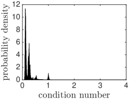
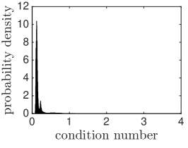
Refer to caption
Refer to caption
Refer to caption
Refer to caption
Refer to caption
Refer to caption
acb1𝑎𝑐𝑏1a\leq c\leq b-1a<c<b1𝑎𝑐𝑏1a<c<b-1c=a𝑐𝑎c=a\;or c=b1𝑐𝑏1\;c=b-1
Figure 6: Condition C1𝐶1C1: condition number 1μ1𝜇\frac{1}{\mu} of the network and its decomposition to two cases for random initialization and learned weights. Top: random initialization Bottom: learned weights. Left: distribution of all combinations of acb1𝑎𝑐𝑏1a\leq c\leq b-1. Middle: when a<c<b1𝑎𝑐𝑏1a<c<b-1. Right: when c=a𝑐𝑎c=a or c=b1𝑐𝑏1c=b-1.
Refer to caption
Refer to caption
Refer to caption
Figure 7: Ratio of activations that flip based on the magnitude of perturbation. Left: random initialization. Middle: learned weights. Right: learned weights (zoomed in).
Refer to caption
Refer to caption
Refer to caption
Refer to caption
Figure 8: From left to right: Condition C3𝐶3C3 for random initialization and learned network, output values for random and learned network