Electroweak vacuum stability in presence of singlet scalar dark matter in TeV scale seesaw models

Abstract

We consider singlet extensions of the standard model, both in the fermion and the scalar sector, to account for the generation of neutrino mass at the TeV scale and the existence of dark matter respectively. For the neutrino sector we consider models with extra singlet fermions which can generate neutrino mass via the so called inverse or linear seesaw mechanism whereas a singlet scalar is introduced as the candidate for dark matter. We show that although these two sectors are disconnected at low energy, the coupling constants of both the sectors get correlated at high energy scale by the constraints coming from the perturbativity and stability/metastability of the electroweak vacuum. The singlet fermions try to destabilize the electroweak vacuum while the singlet scalar aids the stability. As an upshot, the electroweak vacuum may attain absolute stability even upto the Planck scale for suitable values of the parameters. We delineate the parameter space for the singlet fermion and the scalar couplings for which the electroweak vacuum remains stable/metastable and at the same time giving the correct relic density and neutrino masses and mixing angles as observed.

I Introduction

The Large Hadron Collider (LHC) experiment has completed the hunt for the last missing piece of the Standard Model (SM) with the discovery of the Higgs boson Chatrchyan:2012xdj ; Aad:2012tfa . The Higgs boson holds a special status in the SM as it gives mass to all the other particles, with the exception of the neutrino. However, observation of neutrino oscillation, from solar, atmospheric, reactor and accelerator experiments necessitates the extension of the SM to incorporate small neutrino masses. The seesaw mechanism is considered to be the most elegant way to generate small neutrino masses. The origin of seesaw is from the dimension 5 effective operator $\kappa LLHH$, proposed by Weinberg in weinberg . Here, $L$ and $H$ are the SM lepton, and Higgs fields respectively. $\kappa$ is a coupling constant with inverse mass dimension. This term violates lepton number by two units and imply that neutrinos are Majorana particles. The generation of the effective dimension 5 operator needs extension of the SM by new particles. The most minimal scenario in this respect is the canonical type-1 seesaw model, in which the SM is extended by heavy right handed Majorana neutrinos for ultra-violet completion of the theory Minkowski:1977sc ; seesaw1 ; seesaw2 ; Mohapatra:1979ia . The essence of seesaw mechanism lies in the fact that the lepton number is explicitly violated at a high-energy scale which defines the scale of the new physics. However to give an observed neutrino mass of the order of $m_{\nu}\sim 0.01eV$ one needs the Majorana neutrinos to be very heavy ($\sim 10^{15}$ GeV), close to the scale of Grand Unification. However since such high scales are not accessible to colliders, in the context of the LHC, there have been a proliferation of studies involving TeV scale seesaw models. For recent reviews see for instance Boucenna:2014zba ; Deppisch:2015qwa . For ordinary seesaw mechanism lowering the scale of new physics to TeV requires small Yukawa couplings ${\cal{O}}(10^{-6})$ and for such values, the light-heavy mixing is small and no interesting collider signals can be studied. One of the ways to reduce the scale of new physics to TeV is to decouple the new physics scale from the scale of lepton number violation. The smallness of the neutrino mass can then be attributed to small lepton number violating terms. A tiny value of the latter is deemed natural, since when this parameter is zero, the global U(1) lepton number symmetry is reinstated and neutrinos are massless. One of the most popular TeV scale seesaw models based on the above idea is the inverse seesaw model Mohapatra:1986bd . This contains additional singlet states ($\nu_{s}$), along with the right handed neutrinos ($N_{R}$), having opposite lepton numbers. The lepton number is broken softly by introducing a small Majorana mass term for the singlets. This parameter is responsible for the smallness of the neutrino mass and one does not require small Yukawa couplings to get observed neutrino masses and at the same time the scale of new physics can be at TeV. Another possibility of a TeV scale singlet seesaw model is the linear seesaw model Gu:2010xc ; Zhang:2009ac ; Hirsch:2009mx . The difference is, in this case, a small lepton number violating term is generated by the coupling between the the left-handed neutrinos and the singlets states. The inverse seesaw and linear seesaw differ from each other in the way lepton number violation is introduced in the model, as we will see in the next section. Also, the particle content of the minimal models that agree with the oscillation data for these two are different. For linear seesaw, we need only one $N_{R}$ and one $\nu_{s}$ Gavela:2009cd ; Khan:2012zw ; Bambhaniya:2014kga whereas in the inverse seesaw case, we need two $N_{R}$ and two $\nu_{s}$ Malinsky:2009df . Note that the minimal linear seesaw model is the simplest re-constructable Tev scale seesaw model having a minimum number of independent parameters.

Apart from neutrino mass, another issue that requires extension of the SM is the existence of dark matter. Measurements by Planck and WMAP demonstrate that nearly 85 percent of the Universe’s matter density is dark Ade:2015xua . Among the various models of dark matter that are proposed in the literature, the most minimal renormalizable extension of the SM are the so called Higgs portal models Silveira:1985rk ; McDonald:1993ex ; Burgess:2000yq . These models include a scalar singlet that couples only to the Higgs. An additional $Z_{2}$ symmetry is imposed to prevent the decay of the DM and safe-guard its stability. The coupling of the singlet with the Higgs provides the only portal for its interaction with the SM. Nevertheless there can be testable consequences of this scenario which can put constraints on its coupling and mass. These include constraints from searches of invisible decay of Higgs at the Large Hadron Collider (LHC) Belanger:2013xza ; Aad:2015pla ; Khachatryan:2016whc , direct and indirect detections of DM as well as compliance with the observed relic density Dick:2008ah ; Yaguna:2008hd ; Cai:2011kb ; Urbano:2014hda ; Cuoco:2016jqt . Implications for the LHC Barger:2007im ; Cheung:2015dta ; Djouadi:2011aa ; Endo:2014cca ; Han:2016gyy and ILC Ko:2016xwd have also been studied. Combined constraints from all these have been discussed in Mambrini:2011ik ; Cheung:2012xb ; Cline:2013gha and most recently in Athron:2017kgt .

The singlet Higgs can also affect the stability of the electroweak vacuum Gonderinger:2009jp ; EliasMiro:2012ay ; Chen:2012faa ; Khan:2014kba ; Haba:2013lga ; Ghosh:2015apa . It is well known that the electroweak vacuum in the standard model is metastable and the Higgs quartic coupling $\lambda$ is pulled down to negative value by renormalization group running, at an energy of about $10^{9}-10^{10}$ GeV, depending on the value of $\alpha_{s}$ and the top quark mass $m_{t}$, as the dominant contribution comes from the top-Yukawa coupling, $y_{t}$ Alekhin:2012py ; Buttazzo:2013uya . This indicates the existence of another low lying vacuum. If the quartic coupling $\lambda(\mu)$ becomes negative at large renormalization scale $\mu$, it implies that in the early universe the Higgs potential would be unbounded from below and the vacuum would be unstable in that era. But it does not pose any threat to the standard model as it has been shown that the decay time is greater than the age of the universe Isidori:2001bm . In the context of standard model extended with neutrino masses via canonical type-1 seesaw mechanism, the Yukawa coupling of the RH neutrinos also contribute to the RG running, just like $y_{t}$ and thereby we expect it to affect the electroweak vacuum stability negatively. But this effect is not so much because, as discussed before, in order to get the light neutrino masses, either one has to resort to extremely small Yukawa couplings or one needs a very large Majorana mass scale $(\approx 10^{15}\,\textrm{GeV})$ and the contribution to the running of $\lambda$ is much smaller in both the cases compared to that from $y_{t}$. However, for the TeV scale seesaw models, with sizable Yukawa couplings the stability of the vacuum can be altered considerably by the contribution from the neutrinos Rodejohann2012 ; Chakrabortty:2012np ; Khan:2012zw ; Datta:2013mta ; Kobakhidze:2013pya ; Rose:2015fua ; Bambhaniya:2016rbb ; Bambhaniya:2014hla ; Lindner:2015qva . On the other hand, the singlet scalar can help in stabilizing the electroweak vacuum by adding a positive contribution which prevents the Higgs quartic coupling from becoming negative. The stability of the electroweak vacuum in the context of singlet scalar extended SM with an unbroken $Z_{2}$ symmetry has been explored in Gonderinger:2009jp ; Chen:2012faa ; Haba:2013lga ; Khan:2014kba .

In this paper, we extend the SM by adding extra fermion as well as scalar singlets to explain the origin of neutrino mass as well as existence of dark matter . The candidate for dark matter is a real singlet scalar added to SM with an additional $Z_{2}$ symmetry which ensures its stability. For generation of neutrino mass at TeV scale we consider two models. The first one is the general inverse seesaw model with three right handed neutrinos and three additional singlets. The second one is the minimal linear seesaw model. These two sectors are disconnected at the low energy. However, the consideration of the stability of the electroweak vacuum and perturbativity induces a correlation between the two sectors. We study the stability of the electroweak vacuum in this model and explore the effect of the two opposing trends – singlet fermions trying to destabilize the vacuum further and singlet Higgs trying to oppose this. We find the parameter space, which is consistent with the constraints of relic density and neutrino oscillation data and at the same time can cure the instability of the electroweak vacuum. We present some benchmark points for which the electroweak vacuum is stable up to the Planck’s scale. In addition to absolute stability we also explore the parameter region which gives metastability in the context of this model. We investigate the combined effect of these two sectors and obtain the allowed parameter space consistent with observations and vacuum stability/metastability and perturbativity.

The plan of the paper is as follows. In the next section we discuss the TeV scale singlet seesaw models, in particular the inverse seesaw and linear seesaw mechanism. We also outline the diagonalization procedure to give the low energy neutrino mass matrix. In section III we discuss the potential in presence of a singlet scalar. Section IV presents the effective Higgs potential and the renormalization group (RG) evolution of the different couplings. In particular we include the contribution from both fermion and scalar singlets in the effective potential. In section V we discuss the existing constraints on the fermion and the scalar sector couplings from experimental observations and also from perturbativity. We present the results in section VI and conclusions in section VII. .

II TeV scale Singlet Seesaw Models

The most general low scale singlet seesaw scenario consists of adding $m$ right handed neutrinos $N_{R}$ and $n$ gauge-singlet sterile neutrinos $\nu_{s}$ to the standard model. The lepton number for $\nu_{s}$ is chosen to be $-1$ and that for $N_{R}$ is $+1$. For simplicity, we will work in a basis where the charged leptons are identified with their mass eigenstates. We can write the most general Yukawa part of the Lagrangian responsible for neutrino masses, before spontaneous symmetry breaking(SSB) as,

$$-L_{\nu}=\overline{l}_{L}Y_{\nu}\,{H}^{c}N_{R}\,\,+\,\,\overline{l}_{L}Y_{s}\,{H}^{c}\nu_{s}\,\,+\overline{N_{R}^{c}}\,M_{R}\,\nu_{s}\,\,+\,\,\frac{1}{2}\,\overline{\nu_{s}^{c}}M_{\mu}\nu_{s}\,\,\,+\,\,\frac{1}{2}\,\overline{N_{R}^{c}}M_{N}N_{R}\,\,\,+\,\textrm{h.c.}$$ (1)

where $l_{L}$ and $H$ are the lepton and the Higgs doublets respectively, $Y_{\nu}$ and $Y_{s}$ are the Yukawa coupling matrices, $M_{N}$ and $M_{\mu}$ are the symmetric Majorana mass matrices for $N_{R}$ and $\nu_{s}$ respectively. $Y_{\nu}$, $Y_{s}$, $M_{N}$ and $M_{\mu}$ are of dimensions $3\times m,\,3\times n,\,m\times m\,$ and $n\times n$ respectively.

Now, after symmetry breaking, the above equation gives,

$$-L_{mass}=\overline{\nu}_{L}M_{D}N_{R}\,\,+\,\,\overline{\nu}_{L}M_{s}\nu_{s}\,\,+\overline{N_{R}^{c}}\,M_{R}\nu_{s}\,\,+\,\,\frac{1}{2}\,\overline{\nu^{c}_{s}}M_{\mu}\nu_{s}\,\,+\,\,\frac{1}{2}\,\overline{N_{R}^{c}}M_{N}N_{R}\,\,\,+\,\,\,\textrm{h.c.}$$ (2)

where, $M_{D}=Y_{\nu}\langle H\rangle\,$ and $M_{s}=Y_{s}\langle H\rangle\,$. The neutral fermion mass matrix $M$ can be defined as,

$$-L_{mass}=\,\,\ \frac{1}{2}(\,\overline{\nu}_{L}\,\,\,\overline{N_{R}^{c}}\,\,\,\overline{\nu^{c}_{s}}\,)\begin{pmatrix}0&M_{D}&M_{s}\\ M_{D}^{T}&M_{N}&M_{R}\\ M^{T}_{s}&M_{R}^{T}&M_{\mu}\end{pmatrix}\begin{pmatrix}\nu_{L}^{c}\\ N_{R}\\ \nu_{s}\end{pmatrix}\,\,\,+\,\,\,\textrm{h.c.}$$ (3)

From this equation, we can get the variants of the singlet seesaw scenarios by setting certain terms to be zero.

II.1 Inverse Seesaw Model (ISM)

In the inverse seesaw model, $M_{s}$ and $M_{N}$ are taken to be zero Mohapatra:1986bd . The mass scales of the three sub-matrices of $M$ may naturally have a hierarchy $\,M_{R}>>M_{D}>>M_{\mu}\,$, because the mass term $M_{R}$ is not subject to the $SU(2)_{L}$ symmetry breaking and the mass term $M_{\mu}$ violates the lepton number. Thus we can take $M_{\mu}$ to be naturally small by t’ Hooft’s naturalness criteria since the expected degree of lepton number violation in nature is very small. In this paper, we consider a (3+3+3) scenario for the inverse seesaw model for generality and hence all the three sub-matrices $M_{R}$, $M_{D}$ and $M_{\mu}$ are $3\times 3$ matrices. The effective light neutrino mass matrix in the seesaw approximation is given by,

$$M_{light}\,\,=\,\,M_{D}(M_{R}^{T})^{-1}M_{\mu}M_{R}^{-1}M_{D}^{T}$$ (4)

and in the heavy sector, we will have three pairs of degenerate pseudo-Dirac neutrinos of masses of the order $\sim$ $M_{R}\,\pm\,M_{\mu}$. Note that the smallness of $M_{light}$ is naturally attributed to the smallness of both $M_{\mu}$ and $\,\,\frac{M_{D}}{M_{R}}$. For instance, $M_{light}\sim\mathcal{O}\,(0.1)$ eV can easily be achieved for $\,\,\frac{M_{D}}{M_{R}}\sim 10^{-2}\,\,$ and $\,M_{\mu}\sim\mathcal{O}\,$(1) keV. Thus, the seesaw scale can be lowered down considerably assuming $Y_{\nu}\,\sim\,\mathcal{O}(0.1)$, such that $M_{D}\,\sim\,10$ GeV and $M_{R}\,\sim\,1$ TeV.

II.2 Minimal Linear Seesaw Model (MLSM)

In eqn. (3), if we put $M_{N}$ and $M_{\mu}$ to be zero and choose the hierarchy $M_{R}$ $>>$ $M_{D}>>M_{\mu}$, we will get the linear seesaw model Gu:2010xc ; Zhang:2009ac ; Hirsch:2009mx . In this paper, we consider the minimal linear seesaw model in which we add only one right handed neutrino $N_{R}$ and one gauge-singlet sterile neutrino $\nu_{s}$ Gavela:2009cd ; Khan:2012zw ; Bambhaniya:2014kga . In such a case, the lightest neutrino mass is zero. The source of lepton number violation is through the coupling $Y_{s}$ which is assumed to be very small. Here, $Y_{\nu}$ and $Y_{s}$ are the $(3\times 1)$ Yukawa coupling matrices and the overall neutrino mass matrix is a symmetric matrix of dimensions $5\times 5$. The light neutrino mass matrix to the leading order is given by,

$$M_{light}\,=\,M_{D}(M_{R}^{T})^{-1}M_{S}^{T}\,+\,M_{S}(M_{R}^{T})^{-1}{M_{D}^{T}}.$$ (5)

Assuming $M_{D}\,\sim\,100$ GeV and $M_{R}\,\sim\,1$ TeV, one needs $Y_{s}\,\sim\,10^{-11}$ to get light neutrino mass $m_{\nu}\,\sim\,0.1$ eV. The heavy neutrino sector will consist of a pair of degenerate neutrinos.

II.3 Diagonalization of the Seesaw Matrix and Non-unitary PMNS Matrix

The diagonalization procedure is same for both the cases. Here we illustrate it for the inverse seesaw case. The $9\,\times 9$ inverse seesaw mass matrix can be rewritten as,

$$M_{\nu}\,=\,\begin{pmatrix}0&\hat{M}_{D}\\ \hat{M}_{D}^{T}&\hat{M}_{R}\end{pmatrix}$$ (6)

where, $\,\hat{M}_{D}=\,(M_{D}\,\,\,\,0)\,\,$ and $\,\,\hat{M}_{R}=\,\begin{pmatrix}0&M_{R}\\ M_{R}^{T}&M_{\mu}\end{pmatrix}$. We can diagonalize the neutrino mass matrix using a $9\times 9$ unitary matrix Xing:2005kh ; Grimus:2000vj ,

$$U_{0}^{T}\,M_{\nu}\,U\,\,=\,\,M_{\nu}^{diag}$$ (7)

where, $M_{\nu}^{diag}\,=\,\textrm{ diag}\,(m_{1},\,m_{2},\,m_{3},\,M_{1},\,...,\,M_{6})\,$ with mass eigenvalues $\,m_{i}\,(i=1,\,2,\,3)\,$ and $\,M_{j}\,(j=1,\,...,6)\,$ for three light neutrinos and 6 heavy neutrinos respectively. Following the two-step diagonalization procedure, $U_{0}$ could be expressed as, (by keeping terms up to order $\mathcal{O}(\hat{M}_{D}^{2}/\hat{M}_{R}^{2})$) Grimus:2000vj

$$U_{0}=W\,T=\,\begin{pmatrix}U_{L}&V\\ S&U_{H}\end{pmatrix}\,=\,\begin{pmatrix}(1-\frac{1}{2}\epsilon)U_{\nu}&\hat{M}_{D}^{*}(\hat{M}_{R}^{-1})^{*}U_{R}\\ -\hat{M}_{R}^{-1}\hat{M}_{D}^{T}\,U_{\nu}&(1-\frac{1}{2}\epsilon^{\prime})U_{R}\end{pmatrix}.$$ (8)

Here, $\,U_{L},\,V,\,S\,\,\textrm{and}\,\,U_{H}\,$ are $3\times 3\,,\,3\times 6\,,\,6\times 3\,\,\,\textrm{and}\,\,6\times 6\,$ matrices respectively, which are not unitary. W is the matrix which brings the full $9\times 9$ neutrino matrix, in the block diagonal form,

$$W^{T}\begin{pmatrix}0&\hat{M}_{D}\\ \hat{M}_{D}^{T}&\hat{M}_{R}\end{pmatrix}W\,=\,\begin{pmatrix}M_{light}&0\\ 0&M_{heavy}\end{pmatrix},$$ (9)

$T\,=\,\textrm{diag}\,(U_{\nu},U_{R})\,$ diagonalizes the mass matrices in the light and heavy sectors appearing in the upper and lower block of the block diagonal matrix respectively. In the seesaw limit, $M_{light}$ is given by eqn. (4) and $M_{heavy}$ = $\hat{M}_{R}$. In eqn. (8), $U_{L}$ corresponds to the PMNS matrix which acquires a non-unitary correction $(1-\frac{\epsilon}{2})$. The parameters $\epsilon$ and $\epsilon^{\prime}$ characterize the non-unitarity and are given by,

$$\epsilon\,=\,\hat{M}_{D}^{*}\hat{M}_{R}^{-1*}\hat{M}_{R}^{-1}\hat{M}_{D}^{T}\,,$$ (10)

$$\epsilon^{\prime}\,=\,\hat{M}_{R}^{-1}\hat{M}_{D}^{T}\hat{M}_{D}^{*}\hat{M}_{R}^{-1*}.$$ (11)

III Scalar Potential of the Model

As mentioned earlier, in addition to the extra fermions, we also add an extra real scalar singlet $S$ to the standard model. The potential for the scalar sector with an extra $Z_{2}$ symmetry under $S\,\rightarrow\,-S\,$ is given by,

$$V(S,H)\,\,=\,\,{m^{2}}H^{\dagger}H\,+\,\ {\lambda}(H^{\dagger}H)^{2}\,+\,\frac{\kappa}{2}H^{\dagger}H\,S^{2}\,+\,\frac{m_{S}^{2}}{2}S^{2}\,+\,\frac{\lambda_{S}}{24}S^{4}\,.$$ (12)

In this model, we take the vacuum expectation value ($vev$) of $S$ as $0$, so that $Z_{2}$ symmetry is not broken. The standard model scalar doublet $H$ could be written as,

$$H=\frac{1}{\sqrt{2}}\begin{pmatrix}G^{+}\\ v+h+iG^{0}\end{pmatrix}$$ (13)

where the $vev$ $v=246~{}\textrm{GeV}$.

Thus, the scalar sector consists of two particles $h$ and $S$, where $h$ is the standard model Higgs boson with a mass of $\sim$ $126\,GeV$, and the mass of the extra scalar is given by,

$$M_{DM}^{2}\,=\,{m_{S}}^{2}\,+\,\frac{\kappa}{2}v^{2}.$$ (14)

As the $Z_{2}$ symmetry is unbroken upto the Planck scale $M_{pl}=1.22\times 10^{19}$ GeV, the potential can have minima only along the Higgs field direction and also this symmetry prevents the extra scalar from acquiring a vacuum expectation value. This extra scalar field does not mix with the SM Higgs. Also an $odd$ number of this extra scalar does not couple to the standard model particles and the new fermions. As a result, this scalar is stable and serve as a viable weakly interacting massive dark matter particle. The scalar field $S$ can annihilate to the SM particles as well as to the new fermions only via the Higgs exchange. So it is called a Higgs portal dark matter.

IV Effective Higgs Potential and RG evolution of the Couplings

The effective Higgs potential and the renormalization group equations are the same for both the linear and the inverse seesaw models. The two models differ only by the way in which a small lepton number violation is introduced in them, whose effect could be neglected in the RG evolution. So, effectively, the RGEs are the same in both the models, the only difference being the dimensions of the Yukawa coupling matrices and the number of heavy neutrinos present in the model.

IV.1 Effective Higgs Potential

The tree level Higgs potential in the standard model is given by,

$$V(H)\,=\,-m^{2}H^{\dagger}H\,+\,\lambda(H^{\dagger}H)^{2}.$$ (15)

This will get corrections from higher order loop diagrams of SM particles. In the presence of the extra singlets, the effective potential will get additional contributions from the extra scalar and the fermions. Thus, we have the one-loop effective Higgs potential $(V_{1}(h))$ in our model as,

$$V_{1}^{SM+S+\nu}(h)\,=\,V_{1}^{SM}(h)\,+\,V_{1}^{S}(h)\,+\,V_{1}^{\nu}(h)$$ (16)

where the one loop contribution to the effective potential due to the standard model particles is given by Casas:1994qy ; Casas:1996aq ,

$$V_{1}^{SM}(h)\,=\,\sum_{i}\frac{n_{i}}{64\pi^{2}}M_{i}^{4}(h)\Bigg{[}\textrm{ln}\,\frac{M_{i}^{2}(h)}{\mu^{2}(t)}\,-\,c_{i}\Bigg{]}.$$ (17)

Here, the index $i$ is summed over all SM particles and $c_{H,G,f}\,=\,3/2$ and $c_{W,Z}\,=\,5/6$, where $H,\,G,\,f,\,W$ and $Z$ stand for the Higgs boson, the Goldstone boson, fermions and $W$ and $Z$ bosons respectively ; $M_{i}(h)$ can be expressed as,

$$M_{i}^{2}(h)\,=\,\kappa_{i}(t)\,h^{2}(t)\,-\,\kappa^{\prime}_{i}(t).$$

The values of $n_{i}$, $\kappa_{i}$ and $\kappa_{i}^{\prime}$ are given in the eqn. (4) in Casas:1994qy . Here $h\,=\,h(t)$ denotes the classical value of the Higgs field, $t$ being the dimensionless parameter related to the running energy scale $\mu$ as $t~{}=~{}log(\mu/M_{Z})$.

The one loop contribution due to the extra scalar is given by Lerner:2009xg ; Gonderinger:2012rd

$$V_{1}^{S}(h)\,=\,\frac{1}{64\pi^{2}}M_{S}^{4}(h)\Bigg{[}\textrm{ln}\,\frac{M_{S}^{2}(h)}{\mu^{2}(t)}\,-\,\frac{3}{2}\Bigg{]}.$$ (18)

where

$$M_{S}^{2}(h)\,=\,m_{S}^{2}(t)\,+\,\kappa(t)h^{2}(t)/2$$

The contribution of the extra neutrino Yukawa coupling to the one loop effective potential can be written as Casas:1999cd ; Khan:2012zw ,

$$V_{1}^{\nu}(h)=-\frac{((M^{\prime{\dagger}}M^{\prime})_{ii})^{2}}{32\pi^{2}}\Bigg{[}\textrm{ln}\,\frac{(M^{\prime{\dagger}}M^{\prime})_{ii}}{\mu^{2}(t)}-\frac{3}{2}\Bigg{]}-\frac{((M^{\prime}M^{\prime{\dagger}})_{jj})^{2}}{32\pi^{2}}\Bigg{[}\textrm{ln}\,\frac{(M^{\prime}M^{\prime{\dagger}})_{jj}}{\mu^{2}(t)}-\frac{3}{2}\Bigg{]}.$$ (19)

Here $M^{\prime}=M_{D}$ for inverse seesaw and $M^{\prime}=(M_{D}\,\,\,M_{s})$ for linear seesaw. Also, $i$ and $j$ run over three light neutrinos and $m$ heavy neutrinos to which the light neutrinos are coupled via Yukawa coupling respectively. In our analysis, we have taken two-loop (one-loop) contributions to the effective potential from the standard model particles (extra singlet scalar and fermions). For $h(t)\,>>\,v$, the effective potential could be approximated as,

$$V_{eff}^{SM+S+\nu}\,=\,\lambda_{eff}(h)\frac{h^{4}}{4}$$ (20)

with

$$\lambda_{eff}(h)\,=\,\lambda_{eff}^{SM}(h)\,+\,\lambda^{S}_{eff}(h)\,+\,\lambda^{\nu}_{eff}(h)$$ (21)

where the standard model contribution is,

$$\lambda_{eff}^{SM}(h)\,=\,e^{4\Gamma(h)}\,[\lambda(\mu=h)\,+\,\lambda_{eff}^{(1)}(\mu=h)\,+\,\lambda_{eff}^{(2)}(\mu=h)\,].$$ (22)

$\lambda_{eff}^{(1)}$ and $\lambda_{eff}^{(2)}$ are the one- and two- loop contributions respectively and their expressions can be found in Buttazzo:2013uya . The contributions due to the extra scalar and the neutrinos are given by

$$\lambda_{eff}^{S}(h)\,=\,e^{4\Gamma(h)}\,\Bigg{[}\frac{\kappa^{2}}{64\pi^{2}}\Bigg{(}\textrm{ln}\frac{\kappa}{2}-\frac{3}{2}\Bigg{)}\Bigg{]}$$ (23)

and

$$\lambda^{\nu}_{eff}(h)\,=\,-\frac{e^{4\Gamma(h)}}{32\pi^{2}}\Bigg{[}(({Y^{\prime}}_{\nu}^{\dagger}{Y^{\prime}}_{\nu})_{ii})^{2}\Bigg{(}\textrm{ln}\,\frac{({Y^{\prime}}_{\nu}^{\dagger}{Y^{\prime}}_{\nu})_{ii}}{2}\,-\frac{3}{2}\,\Bigg{)}\,+\,(({Y^{\prime}}_{\nu}{Y^{\prime}}_{\nu}^{\dagger})_{jj})^{2}\Bigg{(}\textrm{ln}\,\frac{({Y^{\prime}}_{\nu}{Y^{\prime}}_{\nu}^{\dagger})_{jj}}{2}\,-\frac{3}{2}\,\Bigg{)}\,\Bigg{]}$$ (24)

where,

$$\Gamma(h)\,=\,\int_{M_{t}}^{h}\gamma(\mu)\,d\,\textrm{ln}\,\mu.$$ (25)

Here $\gamma(\mu)$ is the anomalous dimension of the Higgs field and in eqn. (24), ${Y^{\prime}}_{\nu}=Y_{\nu}$ for inverse seesaw and ${Y^{\prime}}_{\nu}=(Y_{\nu}\,\,\,Y_{s})$ for linear seesaw. The contribution of the singlet scalar to the anomalous dimension is zero Gonderinger:2009jp and the contribution from the right handed neutrinos at one loop is given in eqn. (33).

IV.2 Renormalization Group evolution of the couplings from $M_{t}$ to $M_{planck}$

We know that the couplings in a quantum field theory get corrections from higher-order loop diagrams and as a result, the couplings run with the renormalization scale. For a coupling $C$, we have the renormalization group equation (RGE),

$$\mu\frac{dC}{d\mu}\,=\,\sum_{i}\frac{\beta_{C}^{(i)}}{(16\pi^{2})^{i}}$$ (26)

where i stands for the $i^{th}$ loop.

We have evaluated the SM coupling constants at the the top quark mass scale and then run them using the RGEs from $m_{t}$ to $M_{planck}$. For this, we have taken into account the various threshold corrections at $M_{t}$ Sirlin:1985ux ; Melnikov:2000qh ; Holthausen:2011aa . All couplings are expressed in terms of the pole masses Bezrukov:2012sa . We have used one-loop RGEs to calculate $g_{1}(M_{t})$ and $g_{2}(M_{t})$ . For $g_{3}(M_{t})$, we use three-loop RGE running of $\alpha_{s}$ where we have neglected the sixth quark contribution and the effect of the top quark has been included using an effective field theory approach. We have also taken the leading term in the four-loop RGE for $\alpha_{s}$. The mismatch between the top pole mass and the $\overline{MS}$ renormalized coupling has been included. This is given by,

$$y_{t}(M_{t})\,=\,\frac{\sqrt{2}M_{t}}{v}\,(1\,+\,\delta_{t}(M_{t}))$$ (27)

where $\delta_{t}(M_{t})$ is the matching correction for $y_{t}$ at the top pole mass, and similarly for $\lambda(M_{t})$ we have,

$$\lambda(M_{t})\,=\,\frac{M_{H}^{2}}{2v^{2}}\,(1\,+\,\delta_{H}(M_{t})).$$ (28)

We have included the QCD corrections upto three loops Melnikov:2000qh , electroweak corrections upto one-loop Hempfling:1994ar ; Schrempp:1996fb and the $O(\alpha\alpha_{s})$ corrections to the matching of top Yukawa and top pole mass Bezrukov:2012sa ; Jegerlehner:2003py . Using these corrections, we have reproduced the couplings at $M_{t}$ as in references Buttazzo:2013uya ; Khan:2014kba .

Now to evaluate the couplings from $M_{t}$ to $M_{planck}$, we have used three-loop RGEs for standard model couplings Buttazzo:2013uya ; Mihaila:2012fm ; Chetyrkin:2012rz ; Zoller:2013mra ; Zoller:2012cv , two-loop RGEs for the extra scalar couplings Haba:2013lga ; Clark:2009dc ; Davoudiasl:2004be and one-loop RGEs for the extra neutrino Yukawa couplings Antusch:2002rr . The one loop RGEs for the scalar quartic couplings and the neutrino Yukawa coupling in our model are given as,

$$\beta_{\lambda} = \frac{27}{100}g_{1}^{4}+\frac{9}{10}g_{1}^{2}g_{2}^{2}+\frac{9}{4}g_{2}^{4}-\frac{9}{5}g_{1}^{2}\lambda-9g_{2}^{2}\lambda+12\lambda^{2}+\kappa^{2}+4T\lambda-4Y$$ (32)

$$\beta_{\kappa}=-\frac{9}{10}g_{1}^{2}\kappa-\frac{9}{2}g_{2}^{2}\kappa+6\lambda\kappa+4\kappa^{2}+2T\kappa$$

$$\beta_{\lambda_{S}}=3\lambda_{S}+12\kappa^{2}$$

$$\beta_{Y_{\nu}}=Y_{\nu}\biggr{(}\frac{3}{2}Y_{\nu}^{\dagger}Y_{\nu}-\frac{3}{2}Y_{l}^{\dagger}Y_{l}+T-\frac{9}{20}g_{1}^{2}-\frac{9}{4}g_{2}^{2}\biggr{)}$$

where,

$$T = \textrm{Tr}(3Y_{u}^{\dagger}Y_{u}+3Y_{d}^{\dagger}Y_{d}+Y_{l}^{\dagger}Y_{l}+Y_{\nu}^{\dagger}Y_{\nu})$$ (33)

$$Y=\textrm{Tr}(3(Y_{u}^{\dagger}Y_{u})^{2}+3(Y_{d}^{\dagger}Y_{d})^{2}+(Y_{l}^{\dagger}Y_{l})^{2}+(Y_{\nu}^{\dagger}Y_{\nu})^{2}).$$

The effect of $\beta$- functions of new particles enters into the SM RGEs at their effective masses.

V Exsiting bounds on the fermionic and the scalar sectors

For the vacuum stability analysis, we need to find the Yukawa and scalar couplings that satisfy the existing experimental and theoretical constraints. These bounds are discussed below.

V.1 Bounds on the fermionic Sector

$\bullet$ Cosmological constraint on the sum of light neutrino masses

The Planck 2015 results put an upper limit on the sum of active light neutrino masses to be Ade:2015xua

$$\Sigma\,=\,m_{1}+m_{2}+m_{3}<0.23\,\textrm{eV}.$$ (34)

$\bullet$ Constraints from Oscillation data

We use the standard parametrization of the PMNS matrix in which,

$$U_{\nu}=\begin{pmatrix}c_{12}c_{13}&s_{12}c_{13}&s13e^{-i\delta}\\ -c_{23}s_{12}-s_{23}s_{13}c_{12}e^{i\delta}&c_{23}c_{12}-s_{23}s_{13}s_{12}e^{i\delta}&s_{23}c_{13}\\ s_{23}s_{12}-c_{23}s_{13}c_{12}e^{i\delta}&-s_{23}c_{12}-c_{23}s_{13}s_{12}e^{i\delta}&c_{23}c_{13}\end{pmatrix}P$$ (35)

where $c_{ij}=cos\theta_{ij}\,\,,\,\,s_{ij}=sin\theta_{ij}$ and the phase matrix $P=\textrm{diag}\,(1,\,e^{i\alpha_{2}},\,e^{i(\alpha_{3}+\delta)})$ contains the Majorana phases. The global analysis Capozzi:2016rtj ; Esteban:2016qun of neutrino oscillation measurements with three light active neutrinos give the oscillation parameters in their $3\sigma$ range, for both normal hierarchy (NH) for which $m_{3}>m_{2}>m_{1}$ and inverted hierarchy (IH) for which $m_{3}>m_{2}>m_{1}$, as below :

$\star$ Mass squared differences

$$\Delta m_{21}^{2}/10^{-5}\textrm{eV}^{2}\,=\,(7.03\rightarrow 8.09)\,\,\,;\,\,\,\,\,\begin{cases}\Delta m_{31}^{2}/10^{-3}\textrm{eV}^{2}\,=\,(2.407\rightarrow 2.643)&\text{NH}\\ \Delta m_{31}^{2}/10^{-3}\textrm{eV}^{2}\,=\,(-2.635\rightarrow-2.399)&\text{IH}\\ \end{cases}$$ (36)

$\star$ Mixing angles

$$\textrm{sin}^{2}\theta_{12}\,=\,(0.271\rightarrow 0.345)\,\,\,;$$ (37)

$$\textrm{sin}^{2}\theta_{23}=\begin{cases}(0.385\rightarrow 0.635)\\ (0.393\rightarrow 0.640)\\ \end{cases}\,\,\,\,\,;\,\,\,\,\,\textrm{sin}^{2}\theta_{13}=\begin{cases}(0.01934\rightarrow 0.02392)&\text{NH}\\ (0.01953\rightarrow 0.02408)&\text{IH}\\ \end{cases}$$ (38)

$\bullet$ Constraints on the non-unitarity of $U_{PMNS}$ = $U_{L}$

The analysis of electroweak precision observables along with various other low energy precision observables put bound on the non-unitarity of light neutrino mixing matrix $U_{L}$ Antusch:2016brq . At 90$\%$ confidence level,

$$|U_{L}U_{L}^{\dagger}|\,=\,\begin{pmatrix}0.9979-0.9998&<10^{-5}&<0.0021\\ <10^{-5}&0.9996-1.0&<0.0008\\ <0.0021&<0.0008&0.9947-1.0\end{pmatrix}.$$ (39)

This also takes care of the constraints coming from various charged lepton flavor violoating decays like $\,l_{i}\rightarrow l_{j}\,\gamma$, among which $\,\,\textrm{Br}(\mu\,\rightarrow e\,\gamma)$ being the one that gives the most severe bound TheMEG:2016wtm ,

$$\textrm{Br}(\mu\,\rightarrow e\,\gamma)\,\,<\,4.2\times 10^{-13}$$ (40)

$\bullet$ Bounds on the heavy neutrino masses

The search for heavy singlet neutrinos at LEP by the L3 collaboration in the decay channel $N\,\rightarrow\,\,e\,W$ showed no evidence of a singlet neutrino in the mass range between $80\,\textrm{GeV}\,(|V_{\alpha i}|^{2}\,\leq\,2\times 10^{-5})$ and $205\,\textrm{GeV}\,(|V_{\alpha i}|^{2}\,\leq\,1)$ Achard:2001qv , $V_{\alpha i}$ being the mixing matrix elements between the heavy and light neutrinos. Heavy singlet neutrinos in the mass range from 3 GeV up to the Z-boson mass $(m_{Z})$ has also been excluded by LEP experiments from Z-boson decay upto $|V_{\alpha i}|^{2}\,\approx\,10^{-5}$ Adriani:1992pq ; Abreu:1996pa ; L3 . These constraints are taken care of in our analysis by keeping the mass of the lightest heavy neutrino to be greater than or equal to 200 GeV.

V.2 Bounds on the Scalar Sector

$\bullet$ Constraints on scalar potential couplings from perturbativity and unitarity

For the radiatively improved Lagrangian of our model to be perturbative, we should have Lee:1977eg ; Cynolter:2004cq ,

$$\lambda(\Lambda)\,<\,\frac{4\pi}{3}\,\,\,;\,\,\,|\kappa(\Lambda)|\,<\,8\pi\,\,\,;\,\,\,|\lambda_{S}(\Lambda)|\,<\,8\pi$$ (41)

at all scales and the values of the couplings at any scale $\Lambda$ are evaluated using the RG equations. The parameters of the scalar potential (see eqn. (12)) of this model are also constrained by the unitarity of the scattering matrix (S-matrix). At very high field values, one can obtain the scattering matrix by using various scalar-scalar, gauge boson-gauge boson, and scalar-gauge boson scattering amplitudes. Using the equivalence theorem equivalence1 ; equivalence2 ; equivalence3 , we have reproduced the scattering matrix (S-matrix) for this model  Cynolter:2004cq . The unitarity demands that the eigenvalues of the S-matrix should be less than $8\pi$. The unitary bounds are given by,

$$\lambda\leq 8\pi\quad{\rm and}\quad\Big{|}12{\lambda}+{\lambda_{S}}\pm\sqrt{16\kappa^{2}+(-12{\lambda}+{\lambda_{S}})^{2}}\Big{|}\leq 32\pi.$$

$\bullet$ Dark matter constraints

The parameter space for the scalar sector should also satisfy the Planck and WMAP imposed dark matter relic density constraint Ade:2015xua ,

$$\Omega_{DM}h^{2}\,=\,0.1198\,\pm\,0.0026.$$ (42)

In addition, the invisible Higgs decay width and the recent direct detection experiments, in particular, the LUX-2016 Akerib:2016vxi data and the indirect Fermi-LAT dataTheFermi-LAT:2015kwa restrict the arbitrary Higgs portal coupling and the dark matter mass Khan:2014kba ; Athron:2017kgt .

Since the extra fermions are heavy ($\gtrsim$ 200 GeV), for low dark matter mass (around 60 GeV), the dominant (more than 75 $\%$) contributions to the relic density is from the $SS\rightarrow b\bar{b}$ channel. The channels $SS\rightarrow V,V^{*}$ also contribute to the relic density where $V$ stands for the vector bosons $W$ and $Z$, $V^{*}$ indicates the virtual particle which can decay into the SM fermions. In this mass region, the value of the Higgs portal coupling $\kappa$ is $\mathcal{O}$($10^{-2}$) to get the relic density in the right ballpark and simultaneously satisfying the other experimental bounds. However, this region is not of much interest to us since such a small coupling will not contribute much to the running of $\lambda$ and hence will not affect the stability of the EW vacuum much. The LUX-2016 data Akerib:2016vxi has ruled out the dark matter mass region $\sim$ $70-500$ GeV.

If we consider $M_{DM}>>M_{t}$, the annihilation cross-section is proportional to $\frac{\kappa^{2}}{M_{DM}^{2}}$, which ensures that the relic density band in $\kappa-M_{DM}$ Khan:2014kba plane is a straight line. In this region, one can get the right relic density if the ratio of dark matter mass to the Higgs portal coupling $\kappa$ is $\sim$ 3300. In this case, the dominant contributions to the dark matter annihilation channel are $SS\rightarrow hh,t\bar{t}$, VV.

We use FeynRules Alloul:2013bka along with micrOMEGAs Belanger:2010gh ; Belanger:2013oya to compute the relic density of the scalar DM. We have checked that the contribution of annihilation into extra fermions is very small. However this could be significant for dark matter mass $\gtrsim$ 2.5 TeV provided the Yukawa couplings are large enough. But, in the stability analysis discussed in section VI.1.2, we will see that the dark matter mass $\gtrsim$ 2.5 TeV requires the value of $\kappa\gtrsim 0.65$ which violates the perturbativity bounds before the Planck scale. Thus, we consider the dark matter mass in the range $\sim$ 500 GeV - 2.5 TeV with $\kappa$ in the range $\sim$ 0.15 to 0.65. It is to be noted that in the presence of the singlet fermions the value of $\kappa$($M_{Z}$) and hence $M_{DM}$ for which the perturbativity is not obeyed will also depend upon the value of Tr $[Y_{\nu}^{\dagger}Y_{\nu}]$. This will be discussed in the next section.

VI Results

In this section, we present our results of the stability analysis of the electroweak vacuum in the two seesaw scenarios. We confine ourselves to the normal hierarchy. The results for the inverted hierarchy are not expected to be very different Khan:2012zw . We have used the package SARAHStaub:2013tta to do the RG analysis in our work.

VI.1 Inverse Seesaw Model

For the inverse seesaw model, the input parameters are the entries of the matrices $Y_{\nu}$, $M_{S}$ and $M_{\mu}$. Here $Y_{\nu}$ is a complex $3\times 3$ matrix. $M_{S}$ is a real $3\times 3$ matrix and $M_{\mu}$ is a $3\times 3$ diagonal matrix with real entries. We vary the entries of various mass matrices in the range $10^{-2}\,<\,M_{\mu}\,<\,1$ keV and $0\,<M_{R}\,<\,5\times 10^{4}$ GeV. This implies a a heavy neutrino mass of maximum upto a few TeV. With these input parameters, we search for parameter sets consistent with the low energy data using the downhill simplex method Press:1996 . We present in table 1, some representative outputs consistent with data for three benchmark points. In this table $Tr[Y_{\nu}Y^{{\dagger}}_{\nu}]$ is an input. As a consistency check, we also give the value of $Br(\mu\rightarrow e~{}\gamma)$.

$$\begin{array}[]{|c|c|c|c|}\hline\cr{\mbox{Parameter}}&BM-I&BM-II&BM-III\\ \hline\cr\Delta m^{2}_{21}/10^{-5}eV^{2}&8.0891&7.8228&7.6277\\ \Delta m^{2}_{31}/10^{-3}eV^{2}&2.4391&2.5046&2.4078\\ \sin^{2}\theta^{L}_{12}&0.2710&0.3429&0.3449\\ \sin^{2}\theta^{L}_{23}&0.3850&0.3850&0.4102\\ \sin^{2}\theta^{L}_{13}&0.0239&0.0229&0.0238\\ \delta_{PMNS}&1.1173&1.4273&1.1715\\ \phi_{1},\phi_{2}&2.5187,2.9377&2.9384,3.1379&0.4264,0.7426\\ m_{i}/10^{-1}~{}eV&0.10,0.13,0.511&0.23,0.25,0.558&0.10,0.13,0.507\\ M_{i}~{}GeV&200.77,200.77,461.159,,&210.01,210.01,487.284,&200.00,200.00,332.993\\ &461.16,1744.67,1744.669&487.28,1451.34,1451.344&332.99,3568.87,3568.869\\ Tr[Y_{\nu}Y^{{\dagger}}_{\nu}]&0.1&0.2&0.3\\ Br(\mu\rightarrow e~{}\gamma)&0.731\times 10^{-16}&0.1\times 10^{-16}&0.13\times 10^{-15}\\ \hline\cr\end{array}$$

Table 1: Output values for three different benchmark points for inverse seesaw model satisfying all the low energy constraints

VI.1.1 Vacuum Stability

In fig.(1), we display the running of the couplings for various benchmark points in the ISM. In fig.(1(a)), we have shown the variation in the running of the Higgs quartic coupling $\lambda$ for different values of Tr $[Y_{\nu}^{\dagger}Y_{\nu}]$ (0, 0.15 and 0.30) for a fixed value of the Higgs portal coupling $\kappa$ = 0.304. We have chosen the DM mass $M_{DM}$=1000 GeV to get the relic density in the right ballpark. As $\lambda_{S}$ doesn’t alter the relic density, we have fixed it’s value at $0.1$ for all the plots in this paper. We can see that for Tr $[Y_{\nu}^{\dagger}Y_{\nu}]=0$ , i.e., without the right handed neutrinos, the EW vacuum remains absolutely stable upto the Planck scale (green line) and for the large values of Tr $[Y_{\nu}^{\dagger}Y_{\nu}]$, the EW vacuum goes towards the instability (Higgs quartic coupling becomes negative around $\Lambda_{I}~{}\sim~{}10^{10}$ GeV (red line) and $\Lambda_{I}~{}\sim~{}10^{8}$ GeV (black line)) region.

In fig.(1(b)), we plot the running of $\lambda$ for a fixed value of Tr $[Y_{\nu}^{\dagger}Y_{\nu}]$ = 0.1 and different sets of $k$ and $~{}M_{DM}$. It is seen that for a larger value of $\kappa=0.45$ with $M_{DM}$ = 1500 GeV, the EW vacuum remains stable upto Planck scale (purple line). For $\kappa=0.304$ with $M_{DM}$ = 1000 GeV, the quartic coupling $\lambda$ (red line) becomes negative around $\Lambda_{I}~{}\sim~{}10^{11}$ GeV and in the absence of the singlet scalar field, i.e., for $\kappa=0$, $\lambda_{S}=0$ (blue line), $\lambda$ becomes negative around $\Lambda_{I}~{}\sim~{}10^{9}$ GeV and the vacuum goes to the metastability region.

In figs.(1(c)) and (1(d)), we have shown the running of all the three scalar quartic couplings, $\lambda,\,\kappa$ and $\lambda_{S}$ and Tr$[Y_{\nu}^{\dagger}Y_{\nu}]$ for $(M_{DM},\,\kappa)$ = (1000 GeV, 0.304) and (1500 GeV, 0.456) respectively. It can be seen that the values of $\lambda_{s}$ and $\kappa$ increases considerably with the energy scale and can reach the perturbativity bound at the Planck scale depending upon the initial values of $\kappa$ and $\lambda_{S}$ at $M_{Z}$. Here for $\lambda_{S}$=0.1, the maximum allowed value of $\kappa$ will be 0.58 from the perturbativity. The value of Tr$[Y_{\nu}^{\dagger}Y_{\nu}]$ increases only slightly with the energy scale and the value of $\lambda_{S}$ increases faster for larger value of $\kappa$.

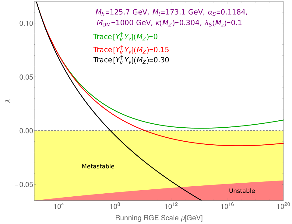
(a) Running of $\lambda$ for different values
of Tr $[Y_{\nu}^{\dagger}Y_{\nu}]$ and a fixed value of $\kappa$

(b) Running of $\lambda$ for a fixed value
of Tr $[Y_{\nu}^{\dagger}Y_{\nu}]$ and different values of $\kappa$

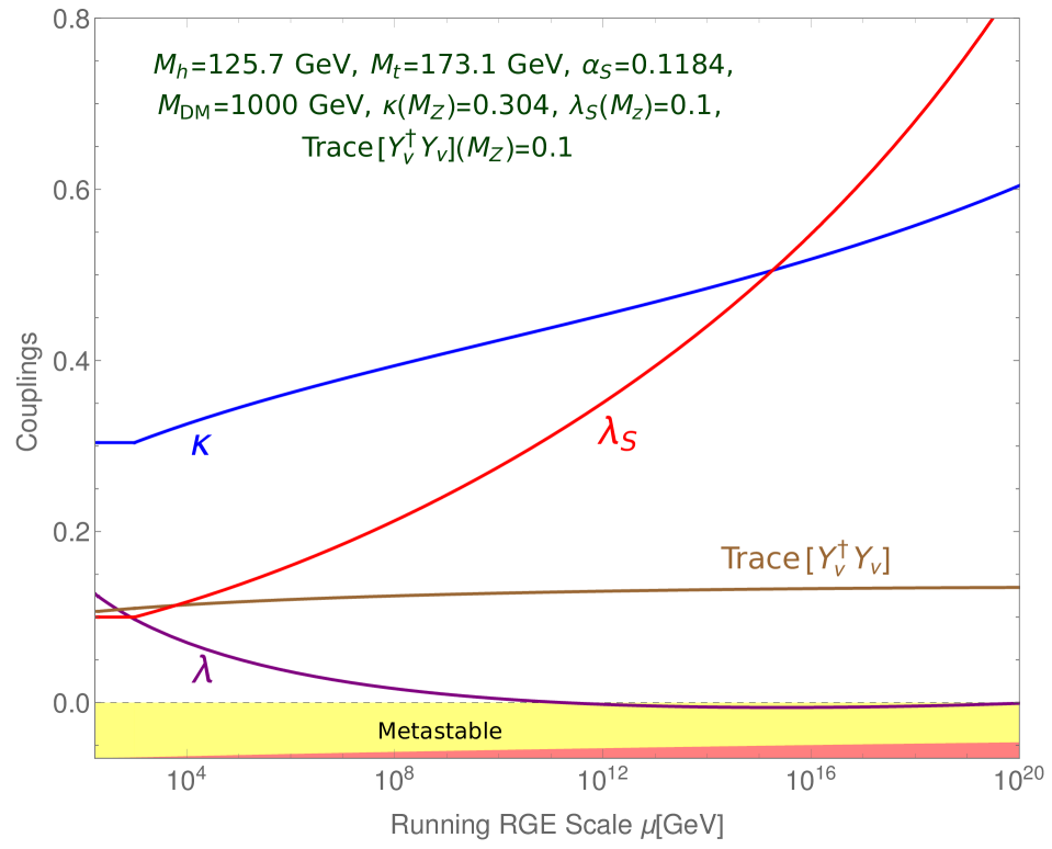
(c) Running of the couplings with energy for dark matter mass of 1000 GeV

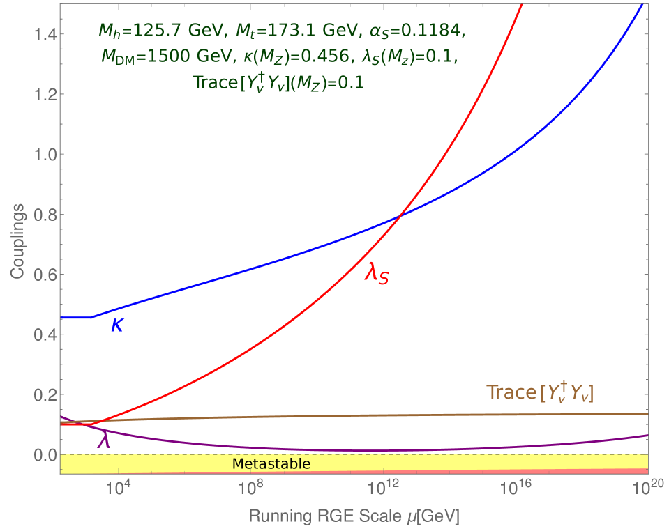
(d) Running of the couplings with energy for dark matter mass of 1500 GeV

Figure 1: Running of the couplings with the energy scale in the Inverse seesaw model

VI.1.2 Tunneling Probability and Phase Diagrams

The present central values of the SM parameters, especially the top Yukawa coupling $y_{t}$ and strong coupling constant $\alpha_{s}$ with Higgs mass $M_{h}\,\approx\,125.7$ GeV suggest that the beta function of the Higgs quartic coupling $\beta_{\lambda}(\equiv dV(h)/dh)$ goes from negative to positive around $10^{15}$ GeV Alekhin:2012py ; Buttazzo:2013uya . This implies that there is an extra deeper minima situated at that scale. So there is a finite probability that the electroweak vacuum might tunnel into that true (deeper) vacuum. But this tunneling probability is not large enough and hence the life time of the EW vacuum remains larger than the age of the universe. This implies that the EW vacuum is metastable in the SM. The expression for the tunneling probability at zero temperature is given by Isidori:2001bm ; Espinosa:2007qp ,

$${\mathcal{P}}_{0}\,=\,V_{U}\,\Lambda_{B}^{4}\,\textrm{exp}\,\Big{(}-\frac{8\pi^{2}}{3\,|\lambda(\Lambda_{B})|}\Big{)}$$ (43)

where $\Lambda_{B}$ is the energy scale at which the action of the Higgs potential is minimum. $V_{U}$ is the volume of the past light cone taken as $\tau_{U}^{4}$, where $\tau_{U}$ is the age of the universe ($\tau_{U}\,=\,4.35\,\times\,10^{17}$ sec)Ade:2015xua . In this work we have neglected the loop corrections and gravitational correction to the action of the Higgs potential Isidori:2007vm . For the vacuum to be metastable, we should have ${\mathcal{P}}_{0}<1$ which implies that Khan:2014kba ,

$$0\,>\,\lambda(\mu)\,>\,\lambda_{min}(\Lambda_{B})\,=\,\frac{-0.06488}{1-0.00986\,\textrm{ln}\,(v/\Lambda_{B})},$$ (44)

whereas the situation $\lambda(\mu)\,<\,\lambda_{min}(\Lambda_{B})$ leads to the unstable EW vacuum. In these regions, $\kappa$ and $\lambda_{S}$ should always be positive to get the scalar potential bounded from below  Khan:2014kba . In our model, the EW vacuum shifts towards stability/instability depending upon the new physics parameter space for the central values of $M_{h}=125.7$ GeV, $M_{t}=173.1$ GeV and $\alpha_{s}=0.1184$ and there might be an extra minima around $10^{12-17}$ GeV.

In fig.(2), we have given the phase diagram in the $\textrm{Tr}\,[Y_{\nu}^{\dagger}Y_{\nu}]\,-\,\kappa$ plane. The line separating the stable region and the metastable region is obtained when the two vacuua are at the same depth, i.e., $\lambda(\mu)\,=\,\beta_{\lambda}(\mu)\,=\,0$. The unstable and the metastable regions are separated by the boundary line where $\beta_{\lambda}(\mu)\,=\,0$ along with $\lambda(\mu)\,=\,\lambda_{min}(\Lambda_{B})$, as defined in eqn. (44). For simplicity, we have plotted fig.(2) (also fig.(1)) by fixing all the eight entries of the $3\times 3$ complex matrix $Y_{\nu}$, but varying only the $(Y_{\nu})_{33}$ element to get a smooth phase diagram.

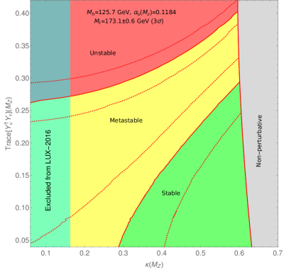
Figure 2: Phase diagram in the Tr$[Y_{\nu}^{\dagger}Y_{\nu}]$ - $\kappa$ plane. We have fixed all the entries of $Y_{\nu}$ except for $(Y_{\nu})_{33}$. The three boundary lines (two dotted and a solid) correspond to $M_{t}\,=\,173.1\,\pm\,0.6$ GeV (3$\sigma$) and we have taken $\lambda_{S}(M_{Z})=0.1$.

From fig. (2), it could be seen that the values of $\kappa$ beyond $\sim$ 0.58 are disallowed by perturbativity bounds and those below $\sim\,0.16$ are disallowed by the direct detection bounds from LUX-2016 Akerib:2016vxi . Note that the vacuum stability analysis of the inverse seesaw model done in reference Rose:2015fua had found that the parameter space with $\textrm{Tr}\,[Y_{\nu}^{\dagger}Y_{\nu}]\,>\,0.4$ were excluded by vacuum metastability constraints. Whereas, in our case, fig.(2) shows that the parameter space with $\textrm{Tr}\,[Y_{\nu}^{\dagger}Y_{\nu}]\,\gtrsim\,0.25$ are excluded for the case when there is no extra scalar. The possible reasons could be that we have kept the maximum value of the heavy neutrino mass to be around a few TeV, whereas the authors of Rose:2015fua had considered heavy neutrinos as heavy as 100 TeV. Obviously, considering larger thresholds would allow us to consider large value of Tr$[Y_{\nu}^{\dagger}Y_{\nu}]$ as the corresponding couplings will enter into RG running only at a higher scale. Another difference with the analysis of Rose:2015fua is that we have fixed 8 of the 9 entries of the Yukawa coupling matrix $Y_{\nu}$. Also, varying all the 9 Yukawa couplings will give us more freedom and the result is expected to change. The main result that we deduce from this plot is the effect of $\kappa$ on the maximum allowed value of Tr $[Y_{\nu}^{\dagger}Y_{\nu}]$, which increases from 0.26 to 0.4 for a value of $\kappa$ as large as 0.6. In addition, we see that the upper bound on $\kappa(M_{Z})$ from perturbativity at the Planck scale decreases from 0.64 to 0.58 as the value of Tr[$Y_{\nu}^{\dagger}Y_{\nu}$] changes from 0 to 0.44. This can be explained from the expression of the $\beta_{\kappa}$ in eqn. (33) which shows that $[Y_{\nu}^{\dagger}Y_{\nu}]$ affect the running $\kappa$ positively through the quantity $T$. Since $M_{DM}$ $\sim$ 3300 $\kappa$ for $M_{DM}>>M_{t}$, the mass of dark matter for which perturbativity is valid, decreases with increase in the value of the Yukawa coupling.

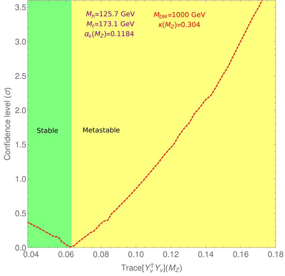
(a) ($\kappa,\,M_{DM}$) = (0.304, 1000 GeV)

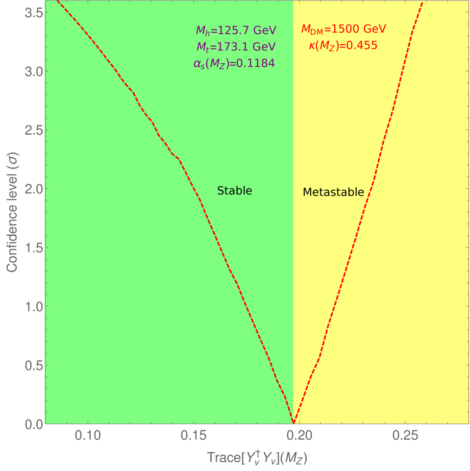
(b) ($\kappa,\,M_{DM}$) = (0.455, 1500 GeV)

Figure 3: Dependence of confidence level at which the EW vacuum stability is excluded/allowed on Tr$[Y_{\nu}^{\dagger}Y_{\nu}]$ for two different values of $\kappa$ and $M_{DM}$. We have taken $\lambda_{S}(M_{Z})=0.1$

VI.1.3 Confidence level of vacuum stability

As we have seen that the stability of the electroweak vacuum changes due to the presence of new physics and hence it becomes important to demonstrate the change in the confidence level at which stability is excluded or allowed (one-sided) Khan:2014kba ; Khan:2015ipa ; Khan:2016sxm . In particular, it will provide a quantitative measurement of (meta)stability in the presence of new physics. In fig.(3), we graphically show how the confidence level at which stability of electroweak vacuum is allowed/excluded depends on new Yukawa couplings of the heavy fermions for the inverse seesaw model in the presence of the extra scalar (dark matter) field. We have plotted the dependence of confidence level against the trace of the Yukawa coupling, Tr$[Y_{\nu}^{\dagger}Y_{\nu}]$ for fixed values of Higgs portal coupling $\kappa\,=\,0.304$ in fig.(3(a)). Here, the dark matter mass $M_{DM}=1000$ GeV is dictated by $\kappa$ to obtain the correct relic density. Similar plot with a higher value of $\kappa=0.455$ with dark matter mass $M_{DM}=1500$ GeV is shown in fig.(3(b)). In this case the electroweak vacuum is absolutely stable for a larger parameter space. For a particular set of values of the model parameters $M_{h}\,=\,125.7$ GeV, $M_{t}\,=\,173.1$ GeV, $\alpha_{s}(M_{z})\,=\,0.1184$ and $\kappa$, the confidence level (one-sided) at which the electroweak vacuum is absolutely stable (green region) decreases with the increase of Tr$[Y_{\nu}^{\dagger}Y_{\nu}]$ and becomes zero for Tr$[Y_{\nu}^{\dagger}Y_{\nu}]=0.06$ in fig.(3(a)) and Tr$[Y_{\nu}^{\dagger}Y_{\nu}]=0.20$ in fig.(3(b)). The confidence level at which the absolute stability of electroweak vacuum is excluded (one-sided) increases with the trace of the Yukawa coupling in the yellow region.

VI.2 Minimal Linear Seesaw Model

In the minimal linear seesaw case, the Yukawa coupling matrices $Y_{\nu}$ and $Y_{s}$ can be completely determined in terms of the oscillation parameters apart from the overall coupling constant $y_{\nu}$ and $y_{s}$ respectively Gavela:2009cd . For normal hierarchy, in MLSM, the Yukawa coupling matrices $Y_{\nu}$ and $Y_{S}$ can be parametrized as,

$$Y_{\nu}\,=\,\frac{y_{\nu}}{\sqrt{2}}\,\Big{(}\sqrt{1+\rho}\,U_{3}^{\dagger}\,+\,\textrm{e}^{i\frac{\pi}{2}}\sqrt{1-\rho}\,U_{2}^{\dagger}\Big{)}$$ (45)

$$Y_{s}\,=\,\frac{y_{s}}{\sqrt{2}}\,\Big{(}\sqrt{1+\rho}\,U_{3}^{\dagger}\,+\,\textrm{e}^{i\frac{\pi}{2}}\sqrt{1-\rho}\,U_{2}^{\dagger}\Big{)}$$ (46)

where

$$\rho\,=\,\frac{\sqrt{1+r}-\sqrt{r}}{\sqrt{1+r}+\sqrt{r}}.$$ (47)

Here, $U_{i}$’s are the columns of the unitary PMNS matrix $U_{\nu}$ and $r$ is the ratio of the solar and the atmospheric mass squared differences. This parametrization makes the vacuum stability analysis in the minimal linear seesaw model much more easier since there are only two independent parameters $y_{\nu}$ and $M_{N}$ in the fermion sector, where $M_{N}$ is the degenerate mass of the two heavy neutrinos (the value of $y_{s}$ being very small $\mathcal{O}(10^{-11})$). A detailed analysis has already been performed in reference Khan:2012zw . Here, we are interested in the interplay between the $Z_{2}$ odd singlet scalar and singlet fermions in the vacuum stability analysis.

In fig.(4), we have plotted the running of the Higgs quartic coupling $\lambda$ with the energy scale $\mu$ upto the Planck scale. The figs.(4(a)) and (4(b)) show the running of $\lambda$ for different values of $k$ (0.0, 0.304, 0.456) and $M_{DM}$ (0,1000 GeV, 1500 GeV), for $M_{N}$=200 GeV and $M_{N}$ = $10^{4}$ GeV respectively for a fixed value of $y_{\nu}^{2}$=0.1. Comparing these two plots, we can see that $\lambda$ tends to go to the instability region faster for smaller values of the heavy neutrino mass. So, the EW vacuum is more stable for larger values of $M_{N}$, because the effect of extra singlet fermion in the running of $\lambda$ enters at a higher value. We also find that as the value of $\kappa$ increases from 0 to 0.304, the electroweak vacuum becomes metastable at a higher value of the energy scale. For $\kappa$=0.456 the electroweak vacuum becomes stable upto the Planck scale even in the presence of the singlet fermions.

Figs.(4(c)) and (4(d)) display the running of $\lambda$ for different values of $y_{\nu}^{2}$ (0.0, 0.15, 0.3) and for fixed values of $k$=0.304 and $M_{DM}$=1000 GeV, for $M_{N}$= 200 GeV and for $M_{N}$= $10^{4}$ GeV respectively. It could be seen from these plots that larger the value of $y_{\nu}$, earlier $\lambda$ becomes negative and more is the tendency for the EW vacuum to be unstable as expected. We note from these two figures that for $\kappa$=0.304, absolute stability is attained only for $y_{\nu}$=0 even in the presence of the singlet scalar.

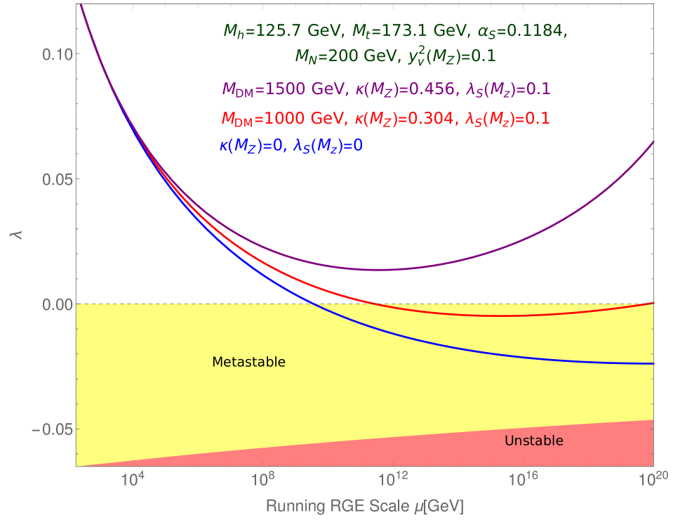
(a)

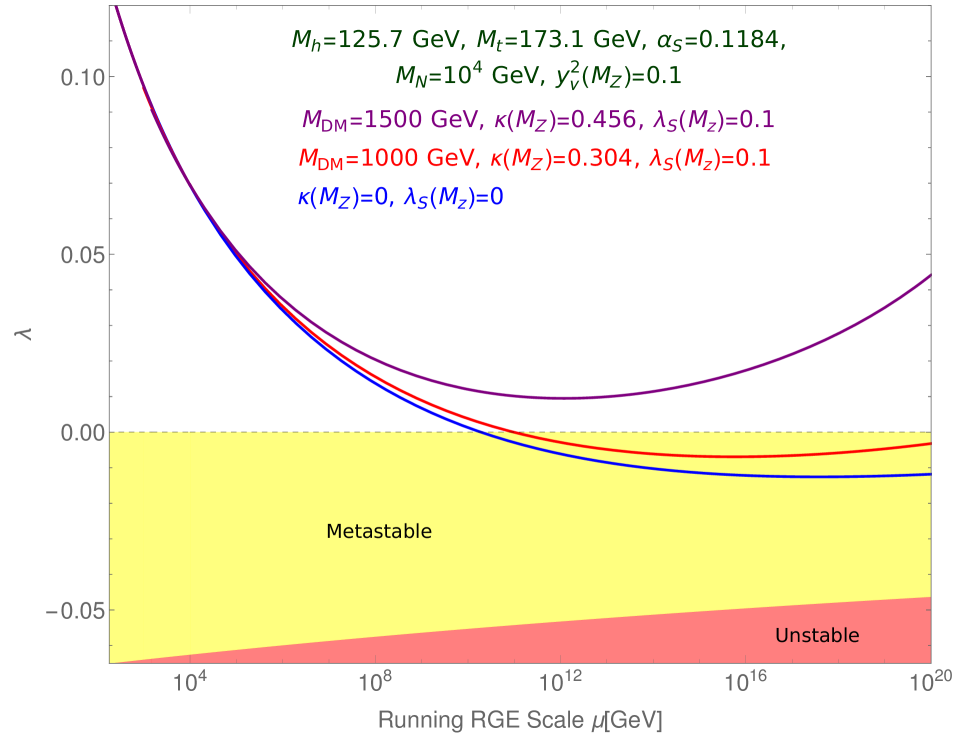
(b)

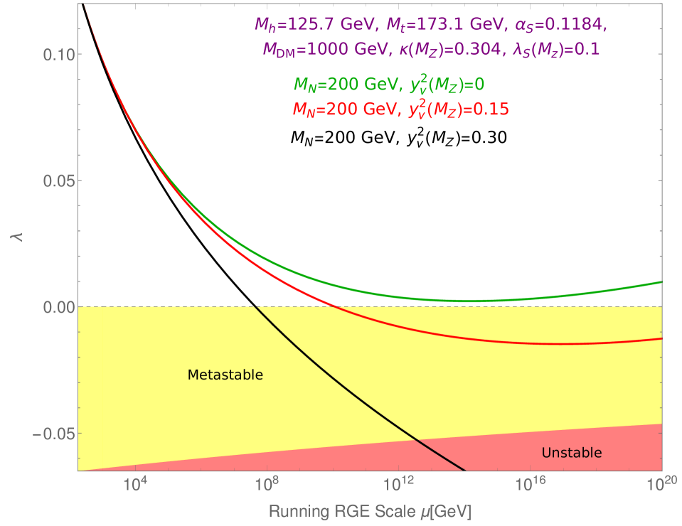
(c)

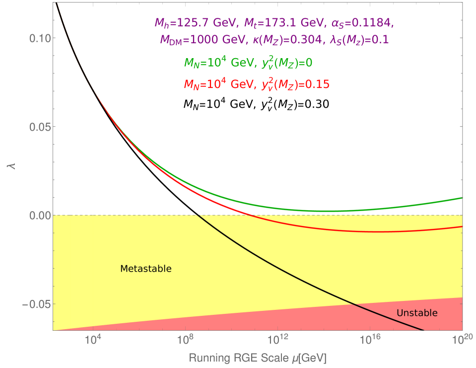
(d)

Figure 4: Running of the quartic coupling $\lambda$ in MLSM with extra scalar for two different values of $M_{N}$. In the upper panel, the three lines are for different values of $M_{DM}$ and $\kappa$ whereas in the lower panel, they are for different values of $y_{\nu}$ and fixed values of $M_{DM}$ and $\kappa$.

In fig.(5), we have shown the phase diagram in the $y_{\nu}\,-\,M_{N}$ plane. The stable (green), unstable (red) and the metastable (yellow) regions are shown and it could be seen that higher the value of $M_{N}$, larger the allowed values of $y_{\nu}$ by vacuum stability as we have discussed earlier. The unstable and the metastable regions are separated by solid red line for the central values of the SM parameters, $M_{h}=125.7$ GeV, $M_{t}=173.1$ GeV and $\alpha_{s}=0.1184$. The red dashed lines represent the 3$\sigma$ variation of the top quark mass. However, we get significant stable region for $M_{h}=125.7$ GeV, $M_{t}=171.3$ GeV and $\alpha_{s}=0.1191$ which corresponds to the solid line separating the stable and the metastable region. The region in the left side of the blue dotted line is disallowed by LFV constraints for the normal hierarchy of light neutrino masses. Fig.(5(a)) is drawn in the absence of the extra scalar and fig.(5(b)) is drawn for ($\kappa,\,M_{DM}$) = (0.304, 1000 GeV). Clearly, there is more stable region in the presence of the extra scalar and the boundary line separating the metastable and the unstable regions also shifts upwards in this case.

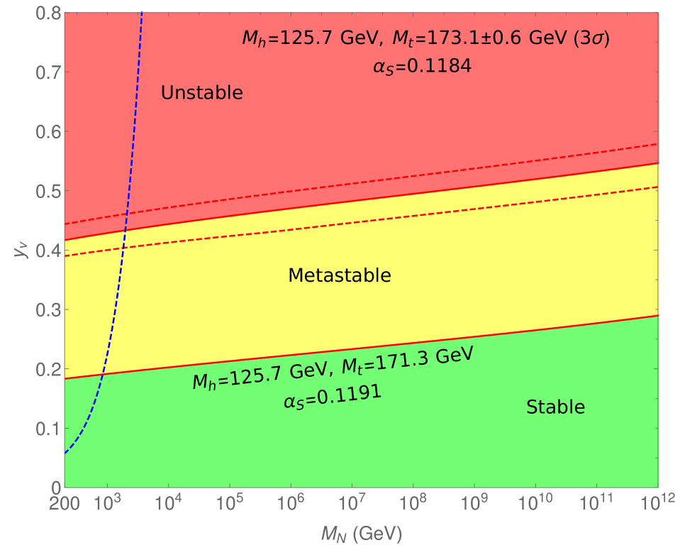
(a) Without the extra scalar

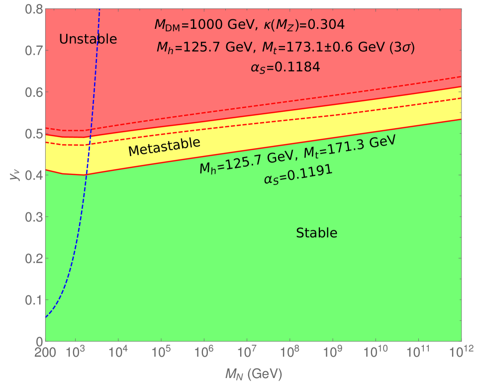
(b) With scalar, ($\kappa,\,M_{DM}$) = (0.304, 1000 GeV)

Figure 5: Phase diagrams in the $y_{\nu}$ - $M_{N}$ plane in the presence and the absence of the extra scalar. Region in the left side of the blue dotted line is disallowed by constraint from BR($\mu\rightarrow e\gamma$). The three boundary lines (two dotted and a solid) correspond to $M_{t}\,=\,173.1\,\pm\,0.6$ GeV (3$\sigma$) and we have taken $\lambda_{S}(M_{Z})=0.1$ in the second plot.

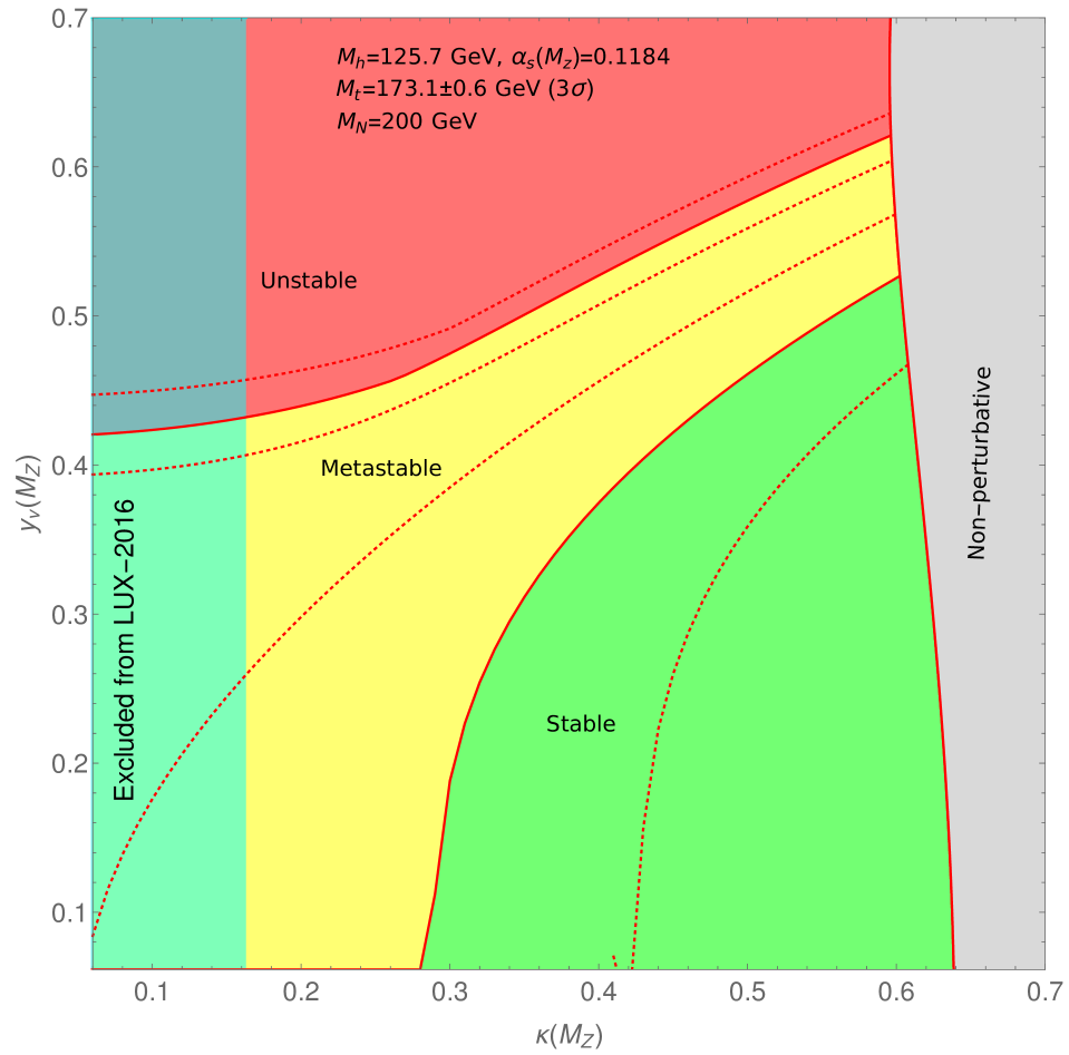
(a)

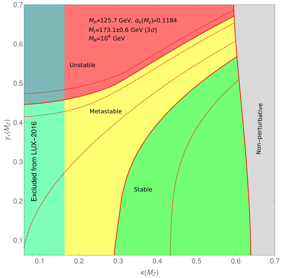
(b)

Figure 6: Phase Diagrams in the $y_{\nu}$ - $\kappa$ plane for two different values of $M_{N}$. Here, $\lambda_{S}(M_{Z})=0.1$.

In fig.(6), we have shown the phase diagrams in the $y_{\nu}$ - $\kappa$ plane for two different values of the heavy neutrino masses : fig.(6(a)) for $M_{N}\,=\,200$ GeV and fig.(6(b)) for $M_{N}\,=\,10^{4}$ GeV. Here also, the red dashed lines represent the 3$\sigma$ variation of top quark mass. It could clearly be seen that as the value of the heavy neutrino mass is higher, the unstable region shifts towards the large values of $y_{\nu}$. This is a result that should be expected from fig.(5). In this model, the theory becomes non-perturbative (grey) for $\kappa$=0.64 for $y_{\nu}$=0.05. The maximum allowed value of $\kappa$ by perturbativity at the Planck scale decreases with increase in $y_{\nu}$ as we have also seen for the inverse seesaw case. The region $\kappa\lesssim 0.16$ is excluded from the recent direct detection experiment at LUX.

VII Conclusions

In this paper we have analysed the stability of the electroweak vacuum in the context of TeV scale inverse seesaw and minimal linear seesaw models extended with a scalar singlet dark matter. We have studied the interplay between the contribution of the extra singlet scalar and the singlet fermions to the EW vacuum stability. We have shown that the coupling constants in these two seemingly disconnected sectors can be correlated at high energy by the vacuum stability/metastability and perturbativity constraints.

In the inverse seesaw scenario, the EW vacuum stability analysis is done after fitting the model parameters with the neutrino oscillation data and non-unitarity constraints on $U_{PMNS}$ (including the LFV constraints from $\mu\rightarrow e\gamma$). For the minimal linear seesaw model, the Yukawa matrix $Y_{\nu}$ can be fully parameterized in terms of the oscillation parameters excepting an overall coupling constant $y_{\nu}$ which can be constrained from vacuum stability and LFV. We have taken the heavy neutrino masses of order upto a few TeV for both the seesaw models. An extra $Z_{2}$ symmetry is imposed to ensure that the scalar particle serves as a viable dark matter candidate. We include all the experimental and theoretical bounds coming from the constraints on relic density and dark matter searches as well as unitarity and perturbativity upto the Planck scale. For the masses of new fermions from 200 GeV to a few TeV, the annihilation cross section to the extra fermions is very small for dark matter mass ${\mathcal{O}}(1-2)$ TeV. We have also checked that the theory violates perturbativity before the Planck scale for DM mass $\gtrsim 2.5$ TeV. In addition we find that the value of the Higgs portal coupling $\kappa$ ($M_{Z}$) for which perturbativity is violated at the Planck scale decreases with increase in the value of the Yukawa couplings of the new fermions. For $M_{DM}>>M_{t}$, one can approximately write $M_{DM}$ $\sim$ 3300 $\kappa$. This implies that with the increasing Yukawa coupling, the mass of dark matter for which the perturbativity is maintained also decreases. Thus the RGE running induces a correlation between the couplings of the two sectors from the perturbativity constraints.

It is well known that the electroweak vacuum of SM is in the metastable region. The presence of the fermionic Yukawa couplings in the context of TeV scale seesaw models drives the vacuum more towards instability while the singlet scalar tries to arrest this tendency. Overall, we find that it is possible to find parameter spaces for which the electroweak vacuum remains absolutely stable for both inverse and linear seesaw models in the presence of the extra scalar particle. We find an upper bound from metastability on Tr$[Y_{\nu}^{\dagger}Y_{\nu}]$ as 0.25 for $\kappa$=0 which increases to 0.4 for $\kappa$=0.6 in inverse seesaw model. We have also seen that in the absence of the extra scalar, the values of the Yukawa coupling $y_{\nu}$ greater than $0.42$ are disallowed in the minimal linear seesaw model. But, in the presence of the extra scalar the values of $y_{\nu}$ up to $\sim 0.6$ are allowed for dark matter mass $\sim 1$ TeV. The correlations between the Yukawa couplings (Tr$[Y_{\nu}^{\dagger}Y_{\nu}]$ or $y_{\nu}$) and $\kappa$ are presented in terms of phase diagrams.

Inverse and linear seesaw models can be explored at LHC through trilepton signatures Bambhaniya:2014kga ; delAguila:2008cj ; Haba:2009sd ; Chen:2011hc ; Das:2012ze ; Bandyopadhyay:2012px ; Das:2014jxa ; Das:2015toa ; Mondal:2016kof . A higher value of Yukawa couplings, as can be achieved in the presence of the Higgs portal dark matter, can facilitate observing such signals at colliders.

References

- [1] Serguei Chatrchyan et al. Observation of a new boson at a mass of 125 GeV with the CMS experiment at the LHC. Phys. Lett., B716:30–61, 2012.
- [2] Georges Aad et al. Observation of a new particle in the search for the Standard Model Higgs boson with the ATLAS detector at the LHC. Phys. Lett., B716:1–29, 2012.
- [3] Steven Weinberg. Baryon- and lepton-nonconserving processes. Phys. Rev. Lett., 43:1566–1570, Nov 1979.
- [4] Peter Minkowski. mu e gamma at a Rate of One Out of 1-Billion Muon Decays? Phys.Lett., B67:421, 1977.
- [5] M. Gell-Mann, P. Ramond, and R. Slansky. Proc.Supergravity Workshop, pages 315–318, 1979.
- [6] T. Yanagida. Workshop on Unified Theory and Baryon Number in the Universe, pages 95–98, 1979.
- [7] Rabindra N. Mohapatra and Goran Senjanovic. Neutrino Mass and Spontaneous Parity Violation. Phys.Rev.Lett., 44:912, 1980.
- [8] Sofiane M. Boucenna, Stefano Morisi, and Jose W. F. Valle. The low-scale approach to neutrino masses. Adv. High Energy Phys., 2014:831598, 2014.
- [9] Frank F. Deppisch, P. S. Bhupal Dev, and Apostolos Pilaftsis. Neutrinos and Collider Physics. New J. Phys., 17(7):075019, 2015.
- [10] Rathin Adhikari and Amitava Raychaudhuri. Light neutrinos from massless texture and below TeV seesaw scale. Phys.Rev., D84:033002, 2011.
- [11] Joern Kersten and Alexei Yu. Smirnov. Right-Handed Neutrinos at CERN LHC and the Mechanism of Neutrino Mass Generation. Phys.Rev., D76:073005, 2007.
- [12] Apostolos Pilaftsis. Radiatively induced neutrino masses and large Higgs neutrino couplings in the standard model with Majorana fields. Z.Phys., C55:275–282, 1992.
- [13] R.N. Mohapatra and J.W.F. Valle. Neutrino Mass and Baryon Number Nonconservation in Superstring Models. Phys.Rev., D34:1642, 1986.
- [14] Pei-Hong Gu and Utpal Sarkar. Leptogenesis with Linear, Inverse or Double Seesaw. Phys.Lett., B694:226–232, 2010.
- [15] He Zhang and Shun Zhou. The Minimal Seesaw Model at the TeV Scale. Phys.Lett., B685:297–301, 2010.
- [16] M. Hirsch, S. Morisi, and J.W.F. Valle. A4-based tri-bimaximal mixing within inverse and linear seesaw schemes. Phys.Lett., B679:454–459, 2009.
- [17] M.B. Gavela, T. Hambye, D. Hernandez, and P. Hernandez. Minimal Flavour Seesaw Models. JHEP, 0909:038, 2009.
- [18] Subrata Khan, Srubabati Goswami, and Sourov Roy. Vacuum Stability constraints on the minimal singlet TeV Seesaw Model. Phys.Rev., D89:073021, 2014.
- [19] Gulab Bambhaniya, Srubabati Goswami, Subrata Khan, Partha Konar, and Tanmoy Mondal. Looking for hints of a reconstructible seesaw model at the Large Hadron Collider. Phys.Rev., D91:075007, 2015.
- [20] Michal Malinsky, Tommy Ohlsson, Zhi-zhong Xing, and He Zhang. Non-unitary neutrino mixing and CP violation in the minimal inverse seesaw model. Phys.Lett., B679:242–248, 2009.
- [21] P. A. R. Ade et al. Planck 2015 results. XIII. Cosmological parameters. Astron. Astrophys., 594:A13, 2016.
- [22] Vanda Silveira and A. Zee. SCALAR PHANTOMS. Phys. Lett., B161:136–140, 1985.
- [23] John McDonald. Gauge singlet scalars as cold dark matter. Phys. Rev., D50:3637–3649, 1994.
- [24] C. P. Burgess, Maxim Pospelov, and Tonnis ter Veldhuis. The Minimal model of nonbaryonic dark matter: A Singlet scalar. Nucl. Phys., B619:709–728, 2001.
- [25] G. Belanger, B. Dumont, U. Ellwanger, J. F. Gunion, and S. Kraml. Global fit to Higgs signal strengths and couplings and implications for extended Higgs sectors. Phys. Rev., D88:075008, 2013.
- [26] Georges Aad et al. Constraints on new phenomena via Higgs boson couplings and invisible decays with the ATLAS detector. JHEP, 11:206, 2015.
- [27] Vardan Khachatryan et al. Searches for invisible decays of the Higgs boson in pp collisions at sqrt(s) = 7, 8, and 13 TeV. JHEP, 02:135, 2017.
- [28] Rainer Dick, Robert B. Mann, and Kai E. Wunderle. Cosmic rays through the Higgs portal. Nucl. Phys., B805:207–230, 2008.
- [29] Carlos E. Yaguna. Gamma rays from the annihilation of singlet scalar dark matter. JCAP, 0903:003, 2009.
- [30] Yi Cai, Xiao-Gang He, and Bo Ren. Low Mass Dark Matter and Invisible Higgs Width In Darkon Models. Phys. Rev., D83:083524, 2011.
- [31] Alfredo Urbano and Wei Xue. Constraining the Higgs portal with antiprotons. JHEP, 03:133, 2015.
- [32] Alessandro Cuoco, Benedikt Eiteneuer, Jan Heisig, and Michael Krämer. A global fit of the -ray galactic center excess within the scalar singlet Higgs portal model. JCAP, 1606(06):050, 2016.
- [33] Vernon Barger, Paul Langacker, Mathew McCaskey, Michael J. Ramsey-Musolf, and Gabe Shaughnessy. LHC Phenomenology of an Extended Standard Model with a Real Scalar Singlet. Phys. Rev., D77:035005, 2008.
- [34] Kingman Cheung, P. Ko, Jae Sik Lee, and Po-Yan Tseng. Bounds on Higgs-Portal models from the LHC Higgs data. JHEP, 10:057, 2015.
- [35] Abdelhak Djouadi, Oleg Lebedev, Yann Mambrini, and Jeremie Quevillon. Implications of LHC searches for Higgs–portal dark matter. Phys. Lett., B709:65–69, 2012.
- [36] Motoi Endo and Yoshitaro Takaesu. Heavy WIMP through Higgs portal at the LHC. Phys. Lett., B743:228–234, 2015.
- [37] Huayong Han, Jin Min Yang, Yang Zhang, and Sibo Zheng. Collider Signatures of Higgs-portal Scalar Dark Matter. Phys. Lett., B756:109–112, 2016.
- [38] P. Ko and Hiroshi Yokoya. Search for Higgs portal DM at the ILC. JHEP, 08:109, 2016.
- [39] Y. Mambrini. Higgs searches and singlet scalar dark matter: Combined constraints from XENON 100 and the LHC. Phys. Rev., D84:115017, 2011.
- [40] Kingman Cheung, Yue-Lin S. Tsai, Po-Yan Tseng, Tzu-Chiang Yuan, and A. Zee. Global Study of the Simplest Scalar Phantom Dark Matter Model. JCAP, 1210:042, 2012.
- [41] James M. Cline, Kimmo Kainulainen, Pat Scott, and Christoph Weniger. Update on scalar singlet dark matter. Phys. Rev., D88:055025, 2013. [Erratum: Phys. Rev.D92,no.3,039906(2015)].
- [42] Peter Athron et al. Status of the scalar singlet dark matter model. 2017.
- [43] Matthew Gonderinger, Yingchuan Li, Hiren Patel, and Michael J. Ramsey-Musolf. Vacuum Stability, Perturbativity, and Scalar Singlet Dark Matter. JHEP, 01:053, 2010.
- [44] Joan Elias-Miro, Jose R. Espinosa, Gian F. Giudice, Hyun Min Lee, and Alessandro Strumia. Stabilization of the Electroweak Vacuum by a Scalar Threshold Effect. JHEP, 06:031, 2012.
- [45] Chian-Shu Chen and Yong Tang. Vacuum stability, neutrinos, and dark matter. JHEP, 04:019, 2012.
- [46] Najimuddin Khan and Subhendu Rakshit. Study of electroweak vacuum metastability with a singlet scalar dark matter. Phys. Rev., D90(11):113008, 2014.
- [47] Naoyuki Haba, Kunio Kaneta, and Ryo Takahashi. Planck scale boundary conditions in the standard model with singlet scalar dark matter. JHEP, 04:029, 2014.
- [48] Swagata Ghosh, Anirban Kundu, and Shamayita Ray. Potential of a singlet scalar enhanced Standard Model. Phys. Rev., D93(11):115034, 2016.
- [49] S. Alekhin, A. Djouadi, and S. Moch. The top quark and Higgs boson masses and the stability of the electroweak vacuum. Phys.Lett., B716:214–219, 2012.
- [50] Dario Buttazzo, Giuseppe Degrassi, Pier Paolo Giardino, Gian F. Giudice, Filippo Sala, Alberto Salvio, and Alessandro Strumia. Investigating the near-criticality of the Higgs boson. JHEP, 12:089, 2013.
- [51] Gino Isidori, Giovanni Ridolfi, and Alessandro Strumia. On the metastability of the standard model vacuum. Nucl.Phys., B609:387–409, 2001.
- [52] Werner Rodejohann and He Zhang. Impact of massive neutrinos on the higgs self-coupling and electroweak vacuum stability. Journal of High Energy Physics, 2012(6):22, 2012.
- [53] Joydeep Chakrabortty, Moumita Das, and Subhendra Mohanty. Constraints on TeV scale Majorana neutrino phenomenology from the Vacuum Stability of the Higgs. Mod. Phys. Lett., A28:1350032, 2013.
- [54] Alakabha Datta, A. Elsayed, S. Khalil, and A. Moursy. Higgs vacuum stability in the extended standard model. Phys. Rev., D88(5):053011, 2013.
- [55] Archil Kobakhidze and Alexander Spencer-Smith. Neutrino Masses and Higgs Vacuum Stability. JHEP, 08:036, 2013.
- [56] Luigi Delle Rose, Carlo Marzo, and Alfredo Urbano. On the stability of the electroweak vacuum in the presence of low-scale seesaw models. 2015.
- [57] Gulab Bambhaniya, P. S. Bhupal Dev, Srubabati Goswami, Subrata Khan, and Werner Rodejohann. Naturalness, Vacuum Stability and Leptogenesis in the Minimal Seesaw Model. Phys. Rev., D95(9):095016, 2017.
- [58] Gulab Bambhaniya, Subrata Khan, Partha Konar, and Tanmoy Mondal. Constraints on a seesaw model leading to quasidegenerate neutrinos and signatures at the LHC. Phys. Rev., D91(9):095007, 2015.
- [59] Manfred Lindner, Hiren H. Patel, and Branimir Radovčić. Electroweak Absolute, Meta-, and Thermal Stability in Neutrino Mass Models. 2015.
- [60] Hooman Davoudiasl, Ryuichiro Kitano, Tianjun Li, and Hitoshi Murayama. The New minimal standard model. Phys. Lett., B609:117–123, 2005.
- [61] Subhaditya Bhattacharya, Sudip Jana, and S. Nandi. Neutrino Masses and Scalar Singlet Dark Matter. Phys. Rev., D95(5):055003, 2017.
- [62] Zhi-zhong Xing and Shun Zhou. Why is the 3 x 3 neutrino mixing matrix almost unitary in realistic seesaw models? HEPNP, 30:828–832, 2006.
- [63] W. Grimus and L. Lavoura. The Seesaw mechanism at arbitrary order: Disentangling the small scale from the large scale. JHEP, 0011:042, 2000.
- [64] J.A. Casas, J.R. Espinosa, and M. Quiros. Improved Higgs mass stability bound in the standard model and implications for supersymmetry. Phys.Lett., B342:171–179, 1995.
- [65] J.A. Casas, J.R. Espinosa, and M. Quiros. Standard model stability bounds for new physics within LHC reach. Phys.Lett., B382:374–382, 1996.
- [66] Rose Natalie Lerner and John McDonald. Gauge singlet scalar as inflaton and thermal relic dark matter. Phys. Rev., D80:123507, 2009.
- [67] Matthew Gonderinger, Hyungjun Lim, and Michael J. Ramsey-Musolf. Complex Scalar Singlet Dark Matter: Vacuum Stability and Phenomenology. Phys. Rev., D86:043511, 2012.
- [68] J. A. Casas, V. Di Clemente, A. Ibarra, and M. Quiros. Massive neutrinos and the Higgs mass window. Phys. Rev., D62:053005, 2000.
- [69] A. Sirlin and R. Zucchini. Dependence of the Quartic Coupling H(m) on M(H) and the Possible Onset of New Physics in the Higgs Sector of the Standard Model. Nucl.Phys., B266:389, 1986.
- [70] Kirill Melnikov and Timo van Ritbergen. The Three loop relation between the MS-bar and the pole quark masses. Phys.Lett., B482:99–108, 2000.
- [71] Martin Holthausen, Kher Sham Lim, and Manfred Lindner. Planck scale Boundary Conditions and the Higgs Mass. JHEP, 1202:037, 2012.
- [72] Fedor Bezrukov, Mikhail Yu. Kalmykov, Bernd A. Kniehl, and Mikhail Shaposhnikov. Higgs Boson Mass and New Physics. JHEP, 1210:140, 2012.
- [73] Ralf Hempfling and Bernd A. Kniehl. On the relation between the fermion pole mass and MS Yukawa coupling in the standard model. Phys.Rev., D51:1386–1394, 1995.
- [74] Barbara Schrempp and Michael Wimmer. Top quark and Higgs boson masses: Interplay between infrared and ultraviolet physics. Prog.Part.Nucl.Phys., 37:1–90, 1996.
- [75] F. Jegerlehner and M. Yu. Kalmykov. O(alpha alpha(s)) correction to the pole mass of the t quark within the standard model. Nucl.Phys., B676:365–389, 2004.
- [76] Luminita N. Mihaila, Jens Salomon, and Matthias Steinhauser. Gauge Coupling Beta Functions in the Standard Model to Three Loops. Phys.Rev.Lett., 108:151602, 2012.
- [77] K.G. Chetyrkin and M.F. Zoller. Three-loop -functions for top-Yukawa and the Higgs self-interaction in the Standard Model. JHEP, 1206:033, 2012.
- [78] Max Zoller. Beta-function for the Higgs self-interaction in the Standard Model at three-loop level. PoS, EPS-HEP2013:322, 2013.
- [79] M. F. Zoller. Vacuum stability in the SM and the three-loop -function for the Higgs self-interaction. Subnucl. Ser., 50:557–566, 2014.
- [80] T. E. Clark, Boyang Liu, S. T. Love, and T. ter Veldhuis. The Standard Model Higgs Boson-Inflaton and Dark Matter. Phys. Rev., D80:075019, 2009.
- [81] Stefan Antusch, Joern Kersten, Manfred Lindner, and Michael Ratz. Neutrino mass matrix running for nondegenerate seesaw scales. Phys.Lett., B538:87–95, 2002.
- [82] Florian Staub. SARAH 4 : A tool for (not only SUSY) model builders. Comput. Phys. Commun., 185:1773–1790, 2014.
- [83] F. Capozzi, E. Lisi, A. Marrone, D. Montanino, and A. Palazzo. Neutrino masses and mixings: Status of known and unknown parameters. Nucl. Phys., B908:218–234, 2016.
- [84] Ivan Esteban, M. C. Gonzalez-Garcia, Michele Maltoni, Ivan Martinez-Soler, and Thomas Schwetz. Updated fit to three neutrino mixing: exploring the accelerator-reactor complementarity. JHEP, 01:087, 2017.
- [85] Stefan Antusch and Oliver Fischer. Probing the nonunitarity of the leptonic mixing matrix at the CEPC. Int. J. Mod. Phys., A31(33):1644006, 2016.
- [86] A. M. Baldini et al. Search for the Lepton Flavour Violating Decay with the Full Dataset of the MEG Experiment. 2016.
- [87] P. Achard et al. Search for heavy isosinglet neutrino in annihilation at LEP. Phys.Lett., B517:67–74, 2001.
- [88] O. Adriani et al. Search for isosinglet neutral heavy leptons in Z0 decays. Phys.Lett., B295:371–382, 1992.
- [89] P. Abreu et al. Search for neutral heavy leptons produced in Z decays. Z.Phys., C74:57–71, 1997.
- [90] M. Z. Akrawy et al. Limits on neutral heavy lepton production from Z0 decay. Phys. Lett., B247:448–457, 1990.
- [91] Benjamin W. Lee, C. Quigg, and H. B. Thacker. Weak Interactions at Very High-Energies: The Role of the Higgs Boson Mass. Phys. Rev., D16:1519, 1977.
- [92] G. Cynolter, E. Lendvai, and G. Pocsik. Note on unitarity constraints in a model for a singlet scalar dark matter candidate. Acta Phys. Polon., B36:827–832, 2005.
- [93] Yao Y. P. and Yuan C. P. Modification of the Equivalence Theorem Due to Loop Corrections. Phys. Rev., D38:2237, 1988.
- [94] Veltman H. G. J. The Equivalence Theorem. Phys. Rev., D41:2294, 1990.
- [95] He H. J. On the precise formulation of equivalence theorem. Phys. Rev., D69:2619, 1992.
- [96] D. S. Akerib et al. Results from a search for dark matter in the complete LUX exposure. Phys. Rev. Lett., 118(2):021303, 2017.
- [97] M. Ajello et al. Fermi-LAT Observations of High-Energy -Ray Emission Toward the Galactic Center. Astrophys. J., 819(1):44, 2016.
- [98] Adam Alloul, Neil D. Christensen, Céline Degrande, Claude Duhr, and Benjamin Fuks. FeynRules 2.0 - A complete toolbox for tree-level phenomenology. Comput. Phys. Commun., 185:2250–2300, 2014.
- [99] G. Belanger, F. Boudjema, P. Brun, A. Pukhov, S. Rosier-Lees, P. Salati, and A. Semenov. Indirect search for dark matter with micrOMEGAs2.4. Comput. Phys. Commun., 182:842–856, 2011.
- [100] G. Belanger, F. Boudjema, A. Pukhov, and A. Semenov. : A program for calculating dark matter observables. Comput. Phys. Commun., 185:960–985, 2014.
- [101] W. T. Vetterling W. H. Press, S. A. Teukolsky and B. P. Flannery. Numerical Recipes in Fortran 90, Second Edition. Cambridge Univ, 1996.
- [102] J.R. Espinosa, G.F. Giudice, and A. Riotto. Cosmological implications of the Higgs mass measurement. JCAP, 0805:002, 2008.
- [103] Gino Isidori, Vyacheslav S. Rychkov, Alessandro Strumia, and Nikolaos Tetradis. Gravitational corrections to standard model vacuum decay. Phys. Rev., D77:025034, 2008.
- [104] Najimuddin Khan and Subhendu Rakshit. Constraints on inert dark matter from the metastability of the electroweak vacuum. Phys. Rev., D92:055006, 2015.
- [105] Najimuddin Khan. Exploring Hyperchargeless Higgs Triplet Model up to the Planck Scale. 2016.
- [106] F. del Aguila and J.A. Aguilar-Saavedra. Distinguishing seesaw models at LHC with multi-lepton signals. Nucl.Phys., B813:22–90, 2009.
- [107] Naoyuki Haba, Shigeki Matsumoto, and Koichi Yoshioka. Observable Seesaw and its Collider Signatures. Phys. Lett., B677:291–295, 2009.
- [108] Chien-Yi Chen and P. S. Bhupal Dev. Multi-Lepton Collider Signatures of Heavy Dirac and Majorana Neutrinos. Phys. Rev., D85:093018, 2012.
- [109] Arindam Das and Nobuchika Okada. Inverse seesaw neutrino signatures at the LHC and ILC. Phys. Rev., D88:113001, 2013.
- [110] Priyotosh Bandyopadhyay, Eung Jin Chun, Hiroshi Okada, and Jong-Chul Park. Higgs Signatures in Inverse Seesaw Model at the LHC. JHEP, 01:079, 2013.
- [111] Arindam Das, P. S. Bhupal Dev, and Nobuchika Okada. Direct bounds on electroweak scale pseudo-Dirac neutrinos from TeV LHC data. Phys. Lett., B735:364–370, 2014.
- [112] Arindam Das and Nobuchika Okada. Improved bounds on the heavy neutrino productions at the LHC. Phys. Rev., D93(3):033003, 2016.
- [113] Subhadeep Mondal and Santosh Kumar Rai. Probing the Heavy Neutrinos of Inverse Seesaw Model at the LHeC. Phys. Rev., D94(3):033008, 2016.