Passage of a shock wave through inhomogeneous media and its impact on a gas bubble deformation

Abstract

The paper investigates shock-induced vortical flows within inhomogeneous media of nonuniform thermodynamic properties. Numerical simulations are performed using an Eularian type mathematical model for compressible multi-component flow problems. The model, which accounts for pressure non-equilibrium and applies different equations of state for individual flow components, shows excellent capabilities for the resolution of interfaces separating compressible fluids as well as for capturing the baroclinic source of vorticity generation. The developed finite volume Godunov type computational approach is equipped with an approximate Riemann solver for calculating fluxes and handles numerically diffused zones at flow component interfaces. The computations are performed for various initial conditions and are compared with available experimental data. The initial conditions promoting a shock-bubble interaction process include: weak to high planar shock waves with a Mach number ranging from $1.2$ to $3$ and isolated cylindrical bubble inhomogeneities of helium, argon, nitrogen, krypton and sulphur hexafluoride. The numerical results reveal the characteristic features of the evolving flow topology. The impulsively generated flow perturbations are dominated by the reflection and refraction of the shock, the compression and acceleration as well as the vorticity generation within the medium. The study is further extended to investigate the influence of the ratio of the heat capacities on the interface deformation.

I Introduction

Compressible multi-component flows with low to high density ratios between components are involved in various physical phenomena and many industrial applications. Some important examples are inertial confinement fusion (ICF) Aglitskiy et al. (2010), rapid and efficient mixing of fuel and oxidizer in supersonic combustion, primary fuel atomization in aircraft engines and droplet breakup. A proper understanding of these flows requires studying the evolution and creation of interfaces resulting from the interaction of a shock wave with the environment of inhomogeneous gases. The diverse flow patterns and the dynamical interaction of gas phases at the interface could cause several physical processes to occur simultaneously. These include shock acceleration or refraction, vorticity generation and its transport, and consequently shock-induced turbulence. The mechanism of these processes is related to the strength and pattern of the propagating shock waves during the short time of their encounter with the surface’s curvatures between flow components and inherently to the difference in the acoustic impedance at the components’ interfaces. The recent review paper Ranjan et al. (2011) provides an excellent description of various possible phenomena occurring during the shock bubble interaction process. When, as a result of the passage of a shock wave, an interface between fluid components is impulsively accelerated, the development of a so called Richtmyer-Meshkov instability (RMI) Brouillette (2002) can be observed. The instability, which directly results from the amplification of perturbations at the interface, is due to baroclinic vorticity generation as a consequence of the misalignment of the pressure gradient of the shock and the local density gradient across the interface. This is a complex phenomenon constituting a challenging task to investigate either experimentally or numerically as the derivation of a mathematical model for this problem is not straightforward.

The nature of the impulsively generated perturbations at the interface of two-component compressible flows has been studied experimentally using idealised configurations. The interaction of a planar shock wave with a cylinder or a sphere is a typical physical arrangement that has received attention. However, the measurement of the entire velocity, density and pressure fields for a large selection of physical scales and interface geometries remains an enormous experimental challenge.

The first key work to monitor the interaction between a plane shock wave and a single gas bubble was presented in Haas and Sturtevant (1987). The shadowgraph photography technique was utilised to visualise a wave front geometry and the deformation of the gas bubble volume. The distortion of a spherical bubble impacted by a plane shock wave was later examined in Layes et al. (2003); Layes and Le Métayer (2007); Layes et al. (2009) using a high speed rotating camera shadowgraph system and in Zhai et al. (2011); Si et al. (2012) by means of the high speed schlieren photography with higher time resolutions. All these experiments were conducted in horizontal shock tubes characterised by a Mach number smaller than $1.7$. Other laser based shock-tube experiments in Ranjan et al. (2007, 2008, 2011); Haehn et al. (2012) covered a wider selection of Mach numbers and provided qualitative and quantitative data for the shock-bubble interaction within the Mach number range of $1.1-3.5$. A similar geometry was investigated in Tomkins et al. (2008) to find a mixing mechanism in a shock-induced instability flow. Although at present it is possible to consider experiments with a higher Mach number by building laboratory facilities based on modern laser technologies, such tests still remain rather difficult and expensive to conduct.

Therefore the development of numerical techniques for these types of applications seems to be an ideal alternative to provide reasonable results at a significantly lower cost. A shock-capturing upwind finite difference numerical method has been utilised to solve the compressible Euler equations for two species in an axisymmetric two-dimensional case of planar shock interacting with a bubble Zabusky and Zeng (1998). The evolution of upstream and downstream complex wave patterns and the appearance of vortex rings were resolved in this study. The experiment in Haas and Sturtevant (1987), in which a shock wave with a Mach number $1.22$ hits a helium bubble, has inspired several other authors Picone and Boris (1988); Quirk and Karni (1996); Bagabir and Drikakis (2001); Banks et al. (2007); Chang and Liou (2007); Terashima and Tryggvason (2009); Hejazialhosseini et al. (2010); Shukla et al. (2010); So et al. (2012); Franquet and Perrier (2012) who adopted this experiment to demonstrate the performance of the numerical techniques they developed. In the majority of the cases the authors used the Euler equations to simulate the experiment and the interface reconstruction was the major task. For example Terashima and Tryggvason (2009) proposed to use the front tracking/ghost fluid method to capture fluid interface minimizing at the same time the smearing of discontinuous variables. In another development Niederhaus et al. (2008) the two-dimensional simulations of the shock-bubble interaction were extended to three spatial dimensions and high Mach numbers using the volume-of-fluid (VOF) method as the numerical approach. The authors considered fourteen different scenarios, including four gas pairings by using a numerical algorithm solving the same system of partial differential equations for each of the two constituent species with an additional numerical scheme for the local interface reconstruction. The 2D VOF method was also used in So et al. (2012). A viscous approach, but without accounting for turbulence, was adopted in the numerical study Giordano and Burtschell (2006) which reproduced different experiments performed in Layes et al. (2003).

The majority of numerical simulations are based on the mixture Euler equations supplemented by two species conservation equations in order to build a reasonable equation of state parameters at the interface (see example Quirk and Karni (1996); Bagabir and Drikakis (2001)). By contrast, the Arbitrary Lagrangian Eulerian methods or Front Tracking Methods Terashima and Tryggvason (2009) consider multi-material interfaces as genuine sharp non-smeared discontinuities. These methods are less flexible when dealing with situations of large interface deformations and topological changes.

The mathematical model advocated by the authors of this paper, is based on a different point of view, and while considering the equations for immiscible fluids, does not require the explicit application of boundary conditions at the interface. The system of equations can be derived from the Baer and Nunziato model Baer and Nunziato (1986). However, in contrast to Franquet and Perrier (2012), who used the original Baer and Nunziato (1986) formulation to investigate shock-bubble interaction, the equations presented in this paper are considered in an asymptotic limit of the velocity relaxation time of the model Baer and Nunziato (1986). This so called “six-equation model”was derived for the first time in Kapila et al. (2001) and was further investigated in Saurel et al. (2009). In the latter reference Saurel et al. (2009) the authors showed that the non-monotonic behaviour of the sound speed which causes errors in the transmission of waves across interfaces can be circumvented by restoring the effects of pressure non-equilibrium in the equation of the volume fraction evolution by using two pressures and their associated pressure relaxation terms. The six-equation model takes advantage of the inherent numerical diffusion at the interface as the necessary condition for interface capturing and avoids the spurious pressure oscillations that frequently occur at the multi-fluid interfaces. Furthermore, and what is of key importance here, the model can naturally handle complex topological changes. The other attractive and desired features of this model could be summarised as follows: the ability to simulate the dynamical creation and the evolution of interfaces, the numerical implementation with a single solver for a system of unified conservation equations and the ability to use different equations of state and hence different heat capacity ratios for individual flow components.

This paper investigates the two-dimensional flow of a shock wave encountering circular inhomogeneities. It presents a numerical study of the interaction of weak to high Mach number waves with an inhomogeneous medium containing a gas bubble. The inherent features of such flow composition are density jumps across the interface. The study concentrates on the early phases of the interaction process. The purpose is to consider the influence of both the Atwood number and the shock wave Mach number on the deformation of the gas bubbles and the associated production of a vorticity field. The physical behaviour of the gas bubbles is monitored using a newly developed numerical algorithm which has been built to solve the six equation model. The considered Atwood numbers are within the range ($-0.8\leqslant A\leqslant 0.7$) and the shock celerity covers the range ($1.2\leqslant\textit{Ma}\leqslant 3$).

The outline of the paper is as follows: section II gives a brief introduction to the two-component flow governing equations. Then in section III the numerical procedures to solve the system are described. The main focus of this paper is section IV, which presents the results of the computational work. First, two independent experimental investigations described in Layes and Le Métayer (2007) and Zhai et al. (2011) are used for the interface evolution validation. In the case of Layes and Le Métayer (2007), a shock wave ($\textit{Ma}=1.5$) interacts with three different air/gas configurations which are air/helium (He), air/nitrogen (N₂) and air/krypton (Kr). In the case of  Zhai et al. (2011) a shock wave ($\textit{Ma}=1.5$) interacts with a sulphur hexafluoride (SF₆) bubble. Second, the study is extended to account for the different gas pairings in an attempt to evaluate the effect of the Atwood number on the complex pattern of the gas bubbles evolution. Third, the effect of the Mach number on the interface evolution is investigated for all cases with the intention to discuss and quantify the production of vorticity resulting from the passage of the shock. Finally, the investigation of the influence of the ratio of the heat capacities on the interface deformation is made. The conclusions are drawn in section V.

II Mathematical model

A two-component compressible flow model is considered. The model consists of two separate, identifiable and interpenetrating continua that are in thermodynamic non-equilibrium with each other. In its one-dimensional mathematical framework the model, first derived in Kapila et al. (2001), consists of six partial differential equations. It constitutes a reduced form of the more general seven equation model Baer and Nunziato (1986). The one dimensional equations of the model are: a statistical volume fraction equation, two continuity equations, one momentum equation and two energy equations. It differs from more popular models which rely on instantaneous pressure equilibrium between the two flow components or phases Murrone and Guillard (2005). The original six-equation model can be expressed in one dimensional space, as follows:

$$\frac{\partial\alpha_{1}}{\partial t}+u\frac{\partial\alpha_{1}}{\partial x}=\mu(p_{1}-p_{2}),$$

$$\frac{\partial\alpha_{1}\rho_{1}}{\partial t}+\frac{\partial\alpha_{1}\rho_{1}u}{\partial x}=0,$$

$$\frac{\partial\alpha_{2}\rho_{2}}{\partial t}+\frac{\partial\alpha_{2}\rho_{2}u}{\partial x}=0,$$

$$\frac{\partial\rho u}{\partial t}+\frac{\partial[\rho u^{2}+(\alpha_{1}p_{1}+\alpha_{2}p_{2})]}{\partial x}=0,$$ (1)

$$\frac{\partial\alpha_{1}\rho_{1}e_{1}}{\partial t}+\frac{\partial\alpha_{1}\rho_{1}e_{1}u}{\partial x}+\alpha_{1}p_{1}\frac{\partial u}{\partial x}=P_{i}\mu(p_{1}-p_{2}),$$

$$\frac{\partial\alpha_{2}\rho_{2}e_{2}}{\partial t}+\frac{\partial\alpha_{2}\rho_{2}e_{2}u}{\partial x}+\alpha_{2}p_{2}\frac{\partial u}{\partial x}=-P_{i}\mu(p_{1}-p_{2}),$$

where $\alpha_{k}$, $\rho_{k}$, $p_{k}$ and $e_{k}$ are respectively the volume fraction, the density, the pressure and the internal energy of the k-th ($1$ or $2$) component of the flow. The volume fractions for both fluids have to satisfy the saturation restriction $\sum\alpha_{k}=1$ and the interfacial pressure $P_{i}$ is defined as $P_{i}=\alpha_{1}p_{1}+\alpha_{2}p_{2}$. Additionally, the mixture density $\rho$, velocity $u$, pressure $p$ and internal energy $e$ are defined as:

$$\rho=\alpha_{1}\rho_{1}+\alpha_{2}\rho_{2},$$

$$u=(\alpha_{1}\rho_{1}u_{1}+\alpha_{2}\rho_{2}u_{2})/\rho,$$

$$p=\alpha_{1}p_{1}+\alpha_{2}p_{2},$$

$$e=(\alpha_{1}\rho_{1}e_{1}+\alpha_{2}\rho_{2}e_{2})/\rho.$$

The $\mu$ variable represents a homogenization parameter controlling the rate at which pressure tends towards equilibrium and it depends on the compressibility of each fluids and their interface topology. Its physical meaning was justified using the second law of thermodynamics Baer and Nunziato (1986). Instead of using only mixture thermodynamic variables, the model (II) keeps two distinct pressures. As a result, the thermodynamic non-equilibrium source term $\mu(p_{1}-p_{2})$ exists in the volume fraction evolution equation and the source term $P_{i}\mu(p_{1}-p_{2})$ in the energy conservation equations.

On the one hand the presence of the left hand side non-conservative terms $\alpha_{k}p_{k}{\partial u}/{\partial x}$ complicates the analytical and computational treatment of the model (II). The non-conservative terms do not allow the governing equations to be written in a divergence form, which is preferred for numerical handling of problems involving shocks. The classical Rankine-Hugoniot relations cannot be defined in an unambiguous manner and additional relations or regularisation procedures must be proposed instead.

On the other hand when dealing with the bubble interface represented by the density jump, these non-conservative terms enable accommodating thermodynamic non-equilibrium effects between the bubble and its surrounding during the passage of shock waves. The pressure non-equilibrium state can be solved using the instantaneous relaxation model with the efficient numerical algorithm proposed in Saurel et al. (2009). This model, while retaining the separate equations of state and pertinent energy equation on both sides of the interfaces, introduces an additional total mixture energy equation. As a result shock waves can be correctly transmitted through the heterogeneous media and the volume fraction positivity in the numerical solution is preserved. This key equation in Saurel et al. (2009) was derived by combining the two internal energy equations with mass and momentum equations. The final form of the total mixture energy equation can be written as:

$$\frac{\partial\rho(Y_{1}e_{1}+Y_{2}e_{2}+\frac{1}{2}u^{2})}{\partial t}\\ +\frac{\partial u(\rho(Y_{1}e_{1}+Y_{2}e_{2}+\frac{1}{2}u^{2})+(\alpha_{1}p_{1}+\alpha_{2}p_{2}))}{\partial x}=0,$$ (2)

where, $Y_{1}$ and $Y_{2}$ are the mass fractions with general form $Y_{k}=\alpha_{k}\rho_{k}/\rho$. The numerical procedures discussed in the next section tackle the overdetermined system of equations consisting of  (II) and (2) and correct the errors resulting from the numerical integration of the non-conservative terms: $\alpha_{k}p_{k}{\partial u}/{\partial x}$. The solution aspects of the overdetermined hyperbolic systems have been considered earlier (see e.g. Godunov (2008)).

The mixture sound speed in this six-equation model has the desired monotonic behaviour as a function of volume and mass fractions and is expressed as:

$$c^{2}=Y_{1}c_{1}^{2}+Y_{2}c_{2}^{2},$$

where, $c_{1}$ and $c_{2}$ are the speeds of sound of the pure fluids.

The model (II) is supplemented by a thermodynamic closure. The ideal gas equation of state, relating the internal energy to the pressure $p=p(\rho,e)$, is used for both flow components experiencing different thermodynamic states. For a given fluid, the equation of state can be written as a pressure law:

$$p_{k}=(\gamma_{k}-1)\rho_{k}e_{k},$$ (3)

where $\gamma_{k}$ is the specific heat ratio for the component $k$ of the flow. Similarly, the mixture equation of state takes the form:

$$p=(\gamma-1)\rho e,$$ (4)

where the specific heat ratio of mixed gas $\gamma$ is calculated from:

$$\frac{1}{\gamma-1}=\sum_{k}\frac{\alpha_{k}}{\gamma_{k}-1}.$$

In this two-component formulation there are no explicit diffusive terms. These terms can be neglected as the diffusive effects do not play a major role in the early stages of bubble-shock interaction. The calculation of the kinematic viscosity of the mixture and estimation of resulting viscous length scales were provided in Picone and Boris (1988); Schilling et al. (2007). The viscosities of the considered fluids are ($\mu\sim 10^{-5}~{}\rm{Pa.s}$) and the evolution is studied over short time scales ($t\leqslant 10^{-3}~{}\rm{s}$).

To tackle two dimensional geometries and two component flows, the original six-equation model (II) can be extended to the following form:

$$\frac{\partial\alpha_{1}}{\partial t}+u\frac{\partial\alpha_{1}}{\partial x}+v\frac{\partial\alpha_{1}}{\partial y}=\mu(p_{1}-p_{2}),$$

$$\frac{\partial\alpha_{1}\rho_{1}}{\partial t}+\frac{\partial\alpha_{1}\rho_{1}u}{\partial x}+\frac{\partial\alpha_{1}\rho_{1}v}{\partial y}=0,$$

$$\frac{\partial\alpha_{2}\rho_{2}}{\partial t}+\frac{\partial\alpha_{2}\rho_{2}u}{\partial x}+\frac{\partial\alpha_{2}\rho_{2}v}{\partial y}=0,$$

$$\frac{\partial\rho u}{\partial t}+\frac{\partial[\rho u^{2}+(\alpha_{1}p_{1}+\alpha_{2}p_{2})]}{\partial x}+\frac{\partial\rho uv}{\partial y}=0,$$ (5)

$$\frac{\partial\rho v}{\partial t}+\frac{\partial\rho uv}{\partial x}+\frac{\partial[\rho v^{2}+(\alpha_{1}p_{1}+\alpha_{2}p_{2})]}{\partial y}=0,$$

$$\frac{\partial\alpha_{1}\rho_{1}e_{1}}{\partial t}+\frac{\partial\alpha_{1}\rho_{1}e_{1}u}{\partial x}+\frac{\partial\alpha_{1}\rho_{1}e_{1}v}{\partial y}+\alpha_{1}p_{1}\frac{\partial u}{\partial x}+\alpha_{1}p_{1}\frac{\partial v}{\partial y}=P_{i}\mu(p_{1}-p_{2}),$$

$$\frac{\partial\alpha_{2}\rho_{2}e_{2}}{\partial t}+\frac{\partial\alpha_{2}\rho_{2}e_{2}u}{\partial x}+\frac{\partial\alpha_{2}\rho_{2}e_{2}v}{\partial y}+\alpha_{2}p_{2}\frac{\partial u}{\partial x}+\alpha_{2}p_{2}\frac{\partial v}{\partial y}=-P_{i}\mu(p_{1}-p_{2}),$$

and

$$\frac{\partial\rho E}{\partial t}+\frac{\partial u(\rho E+(\alpha_{1}p_{1}+\alpha_{2}p_{2}))}{\partial x}+\frac{\partial v(\rho E+(\alpha_{1}p_{1}+\alpha_{2}p_{2}))}{\partial y}=0.$$ (6)

where, $u$ and $v$ represent the components of the velocity in the $x$ and $y$ directions, respectively. The total energy of the mixture for two dimensional flows is given by $E=Y_{1}e_{1}+Y_{2}e_{2}+\frac{1}{2}u^{2}+\frac{1}{2}v^{2}$.

III Numerical method

As stated in the previous section, model (II) cannot be written in a divergence form and hence the standard numerical methods developed for conservation laws are not applied directly here. In order to solve this system a numerical scheme is constructed that decouples the left hand side of model (II) from the pressure relaxation source terms (the right hand side of the model). The left hand side, which represents the advection part of the flow equations, is then analysed to determine the mathematical structure of the system and is rewritten in terms of the primitive variables as follows:

$$\frac{\partial W}{\partial t}+A(W)\frac{\partial W}{\partial x}+B(W)\frac{\partial W}{\partial y}=0,$$ (7)

where the vector of primitive variables $W$, Jacobian matrices $A(W)$ and $B(W)$ for the extended model (II) are:

$$W=\left[\begin{matrix}\alpha_{1}\\ \rho_{1}\\ \rho_{2}\\ u\\ v\\ p_{1}\\ p_{2}\end{matrix}\right],A(W)=\left[\begin{matrix}u&0&0&0&0&0&0\\ 0&u&0&\rho_{1}&0&0&0\\ 0&0&u&\rho_{2}&0&0&0\\ \frac{p_{1}-p_{2}}{\rho}&0&0&u&0&\frac{\alpha_{1}}{\rho}&\frac{1-\alpha_{1}}{\rho}\\ 0&0&0&0&u&0&0\\ 0&0&0&\rho_{1}c_{1}^{2}&0&u&0\\ 0&0&0&\rho_{2}c_{2}^{2}&0&0&u\end{matrix}\right]$$

and

$$B(W)=\left[\begin{matrix}v&0&0&0&0&0&0\\ 0&v&0&0&\rho_{1}&0&0\\ 0&0&v&0&\rho_{2}&0&0\\ 0&0&0&v&0&0&0&\\ \frac{p_{1}-p_{2}}{\rho}&0&0&0&v&\frac{\alpha_{1}}{\rho}&\frac{1-\alpha_{1}}{\rho}\\ 0&0&0&0&\rho_{1}c_{1}^{2}&v&0\\ 0&0&0&0&\rho_{2}c_{2}^{2}&0&v\end{matrix}\right]$$

The seven eigenvalues of the Jacobian matrix $A(W)$ are determined to be: $u-c$, $u$, $u$, $u$, $u$, $u$ and $u+c$. Similarly, the eigenvalues of the Jacobian matrix $B(W)$ are: $v-c$, $v$, $v$, $v$, $v$, $v$ and $v+c$.

III.1 Solution of the hyperbolic part

The above primitive form (7) is hyperbolic but not strictly hyperbolic. Indeed some eigenvalues, which represent the wave speeds, are real but not distinct. The solution of this hyperbolic problem is obtained using the extended Godunov scheme. To achieve second order accuracy the numerical algorithm is equipped with the classical Monotonic Upstream-centered Scheme for Conservation Laws (MUSCL) Toro (1999).

The splitting scheme has been applied to solve the conservative equations on regular meshes. In each time step of simulation ($\Delta t$), the conservative variables evolve in alternate directions $(x,y)$ during time sub-steps ($\Delta t/2$) which are denoted by ($U^{n+1/2}$) and ($U^{n+1}$). The time increment for the 2D second order discretisation of the Godunov scheme takes the following sub-steps:

$$U_{i,j}^{n+1/2}=U_{i,j}^{n}-\frac{\Delta t}{\Delta x}[F^{n}(U^{*}(U_{i+\frac{1}{2},j}^{-},U_{i+\frac{1}{2},j}^{+}))\\ -F^{n}(U^{*}(U_{i-\frac{1}{2},j}^{-},U_{i-\frac{1}{2},j}^{+}))]$$

and

$$U_{i,j}^{n+1}=U_{i,j}^{n+1/2}-\frac{\Delta t}{\Delta y}[G^{n+1/2}(U^{*}(U_{i,j+\frac{1}{2}}^{-},U_{i,j+\frac{1}{2}}^{+}))\\ -G^{n+1/2}(U^{*}(U_{i,j-\frac{1}{2}}^{-},U_{i,j-\frac{1}{2}}^{+}))].$$

The components of the vector $U=[\alpha_{1}\rho_{1},\alpha_{2}\rho_{2},\rho u,\rho v,\rho E]^{T}$ are the conservative variables. $U_{i,j}^{n}$ represents the state vector in a cell ($i,j$) at time $n$ and $U_{i,j}^{n+1}$ represents the state vector at the next time step. $F(U^{*})$ is the flux function in the $x$ direction $F(U)=[\alpha_{1}\rho_{1}u,\alpha_{2}\rho_{2}u,\rho u^{2}+p,\rho uv,u(\rho E+p)]^{T}$. $G(U^{*})$ is the flux function in the $y$ direction $G(U)=[\alpha_{1}\rho_{1}v,\alpha_{2}\rho_{2}v,\rho uv,\rho v^{2}+p,v(\rho E+p)]^{T}$. The superscript “*”refers to the state at each cell boundary. Figure 1 presents a diagram for the flux configurations in two dimensional computations. The plus and minus signs refer to the conservative variable and flux values at cell boundaries in the second order scheme. The second order accuracy is achieved by applying three major steps: the first step consists in the reconstruction of the average local values in each computational cell using extrapolation of piecewise linear approximations, the second step consists in the determination of the variable values at a middle time step and finally the last step is the solution of the Riemann problem. Figure 2 shows the piecewise linear variable variation at the boundaries of each cell. The flux functions in the Godunov scheme are obtained using the approximate Harten, Lax and Van Lear (HLL) Riemann solver Harten et al. (1983); Toro (1999).

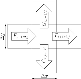
Figure 1: Numerical flux notations within a 2D quadratic mesh.

Figure 2: Schematic diagram representing notations at each computational cell for the piecewise linear variable states (dash line) in the second order scheme.

Figure 3 shows a schematic diagram of the typical wave configuration in the approximate HLL Riemann solver. The wave speeds $S^{R}$ and $S^{L}$ are the boundaries of three characteristics regions: left region ($U_{L}$), right region ($U_{R}$) and the star region ($U^{HLL}$). In this Riemann solver, the second order numerical flux functions in the star region at each cell boundary are written as:

$$F_{i+\frac{1}{2},j}=\left\{\begin{array}[]{ll}F_{i,j}&\mbox{if $0\leq S_{i+\frac{1}{2},j}^{L}$},\\ \frac{S_{i+\frac{1}{2},j}^{R}F_{i,j}-S_{i+\frac{1}{2},j}^{L}F_{i+1,j}+S_{i+\frac{1}{2},j}^{R}S_{i+\frac{1}{2},j}^{L}(U_{i+1,j}-U_{i,j})}{S_{i+\frac{1}{2},j}^{R}-S_{i+\frac{1}{2},j}^{L}}&\mbox{if $S_{i+\frac{1}{2},j}^{L}\leq 0\leq S_{i+\frac{1}{2},j}^{R}$},\\ F_{i+1,j}&\mbox{if $0\geq S_{i+\frac{1}{2},j}^{R}$}.\end{array}\right.$$

$$F_{i-\frac{1}{2},j}=\left\{\begin{array}[]{ll}F_{i-1,j}&\mbox{if $0\leq S_{i-\frac{1}{2},j}^{L}$},\\ \frac{S_{i-\frac{1}{2},j}^{R}F_{i-1,j}-S_{i-\frac{1}{2},j}^{L}F_{i,j}+S_{i-\frac{1}{2},j}^{R}S_{i-\frac{1}{2},j}^{L}(U_{i,j}-U_{i-1,j})}{S_{i-\frac{1}{2},j}^{R}-S_{i-\frac{1}{2},j}^{L}}&\mbox{if $S_{i-\frac{1}{2},j}^{L}\leq 0\leq S_{i-\frac{1}{2},j}^{R}$},\\ F_{i,j}&\mbox{if $0\geq S_{i-\frac{1}{2},j}^{R}$}.\end{array}\right.$$

and

$$G_{i,j+\frac{1}{2}}=\left\{\begin{array}[]{ll}G_{i,j}&\mbox{if $0\leq S_{i,j+\frac{1}{2}}^{L}$},\\ \frac{S_{i,j+\frac{1}{2}}^{R}G_{i,j}-S_{i,j+\frac{1}{2}}^{L}G_{i,j+1}+S_{i,j+\frac{1}{2}}^{R}S_{i,j+\frac{1}{2}}^{L}(U_{i,j+1}-U_{i,j})}{S_{i,j+\frac{1}{2}}^{R}-S_{i,j+\frac{1}{2}}^{L}}&\mbox{if $S_{i,j+\frac{1}{2}}^{L}\leq 0\leq S_{i,j+\frac{1}{2}}^{R}$},\\ G_{i,j+1}&\mbox{if $0\geq S_{i,j+\frac{1}{2}}^{R}$}.\end{array}\right.$$

$$G_{i,j-\frac{1}{2}}=\left\{\begin{array}[]{ll}G_{i,j-1}&\mbox{if $0\leq S_{i,j-\frac{1}{2}}^{L}$},\\ \frac{S_{i,j-\frac{1}{2}}^{R}G_{i,j-1}-S_{i,j-\frac{1}{2}}^{L}G_{i,j}+S_{i,j-\frac{1}{2}}^{R}S_{i,j-\frac{1}{2}}^{L}(U_{i,j}-U_{i,j-1})}{S_{i,j-\frac{1}{2}}^{R}-S_{i,j-\frac{1}{2}}^{L}}&\mbox{if $S_{i,j-\frac{1}{2}}^{L}\leq 0\leq S_{i,j-\frac{1}{2}}^{R}$},\\ G_{i,j}&\mbox{if $0\geq S_{i,j-\frac{1}{2}}^{R}$}.\end{array}\right.$$

Figure 3: Wave configuration at a cell boundary in the approximate HLL Riemann solver with right initial data $(U_{R})$, left initial data $(U_{L})$ and the star region.

Similarly, the splitting scheme is applied in the descritization of non-conservative equations, i.e. the volume fraction and the two energy equations as follows:

$$\alpha_{1i,j}^{n+1/2}=\alpha_{1i,j}^{n}-\frac{\Delta t}{\Delta x}[(u\alpha_{1})_{i+\frac{1}{2},j}^{*}-(u\alpha_{1})_{i-\frac{1}{2},j}^{*}\\ -\alpha_{1i,j}(u_{i+\frac{1}{2},j}^{*}-u_{i-\frac{1}{2},j}^{*})]^{n},$$

$$\alpha_{1i,j}^{n+1}=\alpha^{n+1/2}_{1i,j}-\frac{\Delta t}{\Delta y}[(v\alpha_{1})_{i,j+\frac{1}{2}}^{*}-(v\alpha_{1})_{i,j-\frac{1}{2}}^{*}\\ -\alpha_{1i,j}(v_{i,j+\frac{1}{2}}^{*}-v_{i,j-\frac{1}{2}}^{*})]^{n+1/2},$$

$$(\alpha\rho e)_{ki,j}^{n+1/2}=(\alpha\rho e)_{ki,j}^{n}-\frac{\Delta t}{\Delta x}[(\alpha\rho eu)_{ki+\frac{1}{2},j}^{*}-(\alpha\rho eu)_{ki-\frac{1}{2},j}^{*}\\ +(\alpha p)_{ki,j}(u_{i+\frac{1}{2},j}^{*}-u_{i-\frac{1}{2},j}^{*})]^{n},$$

$$(\alpha\rho e)_{ki,j}^{n+1}=(\alpha\rho e)_{ki,j}^{n+1/2}-\frac{\Delta t}{\Delta y}[(\alpha\rho ev)_{ki,j+\frac{1}{2}}^{*}-(\alpha\rho ev)_{ki,j-\frac{1}{2}}^{*}\\ +(\alpha p)_{ki,j}(v_{i,j+\frac{1}{2}}^{*}-v_{i,j-\frac{1}{2}}^{*})]^{n+1/2},$$

The stability of the numerical method is controlled by the Courant-Friedrichs-Lewy (CFL) number, which imposes a restriction on the time step $\Delta t$ as follows:

$$\Delta t=\text{CFL}\times\text{min}(\frac{\Delta x}{S_{x}},\frac{\Delta y}{S_{y}}),$$ (8)

where $S_{x}$ and $S_{y}$ are the maximum wave speeds in the $x$ and $y$ directions respectively.

$$S_{x}=\text{max}\langle 0,u_{i\pm\frac{1}{2},j}^{+}+c_{i\pm\frac{1}{2},j}^{+},u_{i\pm\frac{1}{2},j}^{-}+c_{i\pm\frac{1}{2},j}^{-}\rangle,$$

$$S_{y}=\text{max}\langle 0,v_{i,j\pm\frac{1}{2}}^{+}+c_{i,j\pm\frac{1}{2}}^{+},v_{i,j\pm\frac{1}{2}}^{-}+c_{i,j\pm\frac{1}{2}}^{-}\rangle.$$

III.2 Solution of the pressure relaxation part

In each time step after the hyperbolic advection part is accomplished, the pressure equilibrium is achieved via the relaxation procedure. The pressure relaxation implies volume variations because of the interfacial pressure work. This represents the solution of the sub-problem governed by the following ordinary differential equations (ODE), with the source term representing the right hand side of the model (II).

$$\frac{\partial\alpha_{1}}{\partial t} = \mu(p_{1}-p_{2}),$$

$$\frac{\partial\alpha_{1}\rho_{1}}{\partial t} = 0,$$

$$\frac{\partial\alpha_{2}\rho_{2}}{\partial t} = 0,$$

$$\frac{\partial\rho u}{\partial t} = 0,$$

$$\frac{\partial\rho v}{\partial t} = 0,$$

$$\frac{\partial\alpha_{1}\rho_{1}e_{1}}{\partial t} = \mu P_{i}(p_{1}-p_{2}),$$

$$\frac{\partial\alpha_{2}\rho_{2}e_{2}}{\partial t} = -\mu P_{i}(p_{1}-p_{2}).$$ (9)

The pressure relaxation is fulfilled instantaneously when the value of $\mu$ in system (II) is assumed to be infinite. To solve the ODE system (9), an iterative method for the pressure relaxation for compressible multiphase flow is implemented. This method is the iterative “procedure 4” described in Lallemand et al. (2005). This step rectifies the calculation of the internal energies to satisfy the second law of thermodynamics. The second amendment comes from solving the extra total energy equation (6), where the mixture pressure is calculated from the mixture equation of state. The overall sequence of the numerical solution steps follows the idea of succession of operators introduced in Strang (1968).

IV Results and Discussion

This section is divided into four parts: In the first part the general description of the physics and the mechanism of the shock-bubble interaction phenomenon are revisited. In the second part the correctness of the results obtained using the developed numerical code is quantified. This is made by validating the numerical results for different shock-bubble interaction scenarios against the experimental data reported in Layes and Le Métayer (2007). In the third and fourth subsections the investigation of the shock-bubble interaction problem is extended to a wider selection of physically intriguing cases for which experimental data are not available.

IV.1 General features of shock-bubble interaction problems

The flow configurations for the studied problems are classified according to the value of the Atwood number $A=(\rho_{b}-\rho_{s})/(\rho_{b}+\rho_{s})$, where $\rho_{b}$ is the density of the bubble and $\rho_{s}$ is the density of the surrounding medium. If the density of the bubble is lower than the density of the surrounding fluid, the value of the Atwood number becomes negative and this case represents heavy/light arrangement. In contrast, if the density of the bubble is higher than the density of the surrounding fluid, the value of the Atwood number becomes positive and this case represents light/heavy arrangement. Alternative terminologies exist and describe these flow configurations as divergent in the case of light bubble or as convergent in the case of heavy bubble Haas and Sturtevant (1987), or fast/slow interface or slow/fast interface according to the sound speed of the flow constituents Zabusky and Zeng (1998).

Figure 4 schematically presents the typical flow configuration during an early stage of the shock-bubble interaction process. The flow patterns of heavy/light, Fig. 4(a), and light/heavy, Fig. 4(b), scenarios show the set of wave configurations associated with the interaction and the deformation of the bubble interface. After hitting the upstream interface of the bubble from the right hand side, the planar shock wave changes its uniform front, which evolves into two parts. One part does not interact directly with the gas filling the bubble while the second one transforms into a transmitted wave interacting with the bubble. In addition a reflected wave, as in the case of a heavy bubble, or a rarefaction wave front, as in the case of a light bubble, does occur and propagates back in the right direction.

Figure 4: Schematic diagram of a shock-bubble interaction flow field and different wave configurations (a) light bubble and (b) heavy bubble. The planar shock moves from right to left.

In the case of a light bubble (i.e. negative $A$ number, Fig. 4(a)), the transmitted shock travels through the gas bubble faster than the incident shock outside the bubble. This is the consequence of the mismatch in flow constituents acoustic impedances ($Z=\rho c$) across the interface. The shock front also takes a divergent shape due to the curvature of the interface and provokes the generation of a set of secondary waves inside and outside the bubble boundary. These secondary waves consist in irregular waves Henderson (1966, 1989). A precursor (refracted) shock wave propagates downstream outside the bubble, internal reflected shocks are generated inside the bubble and move back upstream as the result of the interaction of the transmitted shock with the internal surface of the bubble. A Mach stem shock wave travels outside the bubble. A triple point is formed outside the bubble owing to the intersection of the exterior incident shock, the precursor shock and the Mach stem.

In the case of a heavy bubble (i.e. positive $A$ number, Fig. 4(b)) the scenario is completely different. The difference in the acoustic impedance between the fluids across the interface makes the transmitted shock inside the bubble moving more slowly than the incident shock outside the bubble. The transmitted shock becomes convergent. The interaction of the transmitted shock with the internal surface of the bubble produces a rarefaction wave propagating backward inside the bubble.

To explain the role of acoustic impedance mismatch in the creation of a vorticity field it is convenient to consider the vorticity transport form of the Euler equations. The momentum equation governing the evolution of vorticity is

$$\frac{D\omega}{Dt}=\underbrace{\vphantom{\frac{1}{\rho^{2}}}(\omega\cdot\nabla)\bf{u}}_{\text{stretching}}-\underbrace{\vphantom{\frac{1}{\rho^{2}}}\omega(\nabla\cdot{\bf{u}})}_{\text{dilatation}}+\underbrace{\frac{1}{\rho^{2}}(\nabla\rho\times\nabla p)}_{\text{baroclinicity}}.$$ (10)

This equation contains, in contrast to its 2D counterpart, the term corresponding to vorticity stretching. High resolution shock-induced 3D simulations were performed to analyze the relative importance of stretching, dilatation and baroclinic terms in the vorticity equation at $\textit{Ma}=3$ and $\textit{Ma}=10$ Hejazialhosseini et al. (2013). It was found that the stretching term contribution manifests its existence after initial phases of shock bubble interaction. The only term of importance in the early stages of a shock-bubble interaction for which $\omega$ is initially equal to zero is the baroclinic torque ($\nabla\rho\times\nabla p$). The misalignment of the local pressure and density gradients leads to the non-zero source term in equation (10). Because of the curved surface of the bubble, different parts of the incident planar shock will strike the bubble surface at different times, so the refracted interior wave will be misaligned with the density gradient. The baroclinic torque is the largest where the pressure gradient is perpendicular to the density gradient. Whereas, at the most upstream and downstream poles of the gas bubble, the baroclinic torque is equal to zero, owing to the collinearity of density and pressure gradients. The curvature of the shock wave front (the refracted shock wave) has also been used to build a theory behind the vorticity generation. It originates from the conservation of the tangential velocity and the angular momentum across the shock wave as the compression only affects the motion normal to the shock surface (for details see Kevlahan (1997) and also recent works of  Huete et al. (2011, 2012); Wouchuk and Sano (2015)). The rotational motion starting from zero-vorticity initial conditions distorts the flow field and the shape of the bubble. The lighter density fluid will be accelerated faster than the high density fluid.

IV.2 Validation of shock-single bubble interaction cases

The experimental studies performed in Layes and Le Métayer (2007) and Zhai et al. (2011) constituted validation cases for the numerical approach developed in the present paper. The authors provided sequences of flow structures resulting from experiments and compared them with numerical simulations they also conducted. The mathematical model and numerical technique considered in the present contribution are fundamentally different from the ones utilised in the reference works of Layes and Le Métayer (2007) and Zhai et al. (2011) and hence the main features of their approaches are highlighted.

The authors in Layes and Le Métayer (2007) employed a homogenization method known as the discrete equations method (DEM), which was earlier introduced by Abgrall and Saurel (2003). In this approach the averaged equations for the mixture are not used. Instead the DEM method obtains a well-posed discrete equation system from the single-phase Euler equations by construction of a numerical scheme which uses a sequence of accurate single-phase Riemann solutions. The local interface variables are determined at each two-phase interface. Then, an averaging procedure which enables coupling between the two fluids is applied generating a set of discrete equations that can be used directly as a numerical scheme. The advantage of such an approach is its natural ability to treat correctly the non-conservative terms. In our approach the solution strategy to handle non-conservative terms is different. It requires the usage of an additional conservative equation for the total mixture energy (2). As a result the present model enables a correct transmission of shock waves through the heterogeneous media. The volume fraction positivity in the numerical solution is also preserved.

The authors in Zhai et al. (2011) adopted the 2D axisymmetrical numerical approach of Sun and Takayama (1999) and solved the mixture Euler equations supplemented by one species conservation equation to capture the interface. It is assumed in this approach that the gas components are in pressure equilibrium and move with a single velocity. This assumption restricts the approach to the cases when the density variations between components are moderate.

IV.2.1 Experiments of Layes and Le Métayer Layes and Le Métayer (2007)

These experiments were reproduced numerically for three different cases in which $\textit{Ma}=1.5$ planar shock wave interacts with a helium, nitrogen or krypton cylindrical bubble of a diameter $D_{o}=0.04~{}\rm{m}$ located in a shock tube. The thermodynamic properties of the bubbles and surrounding air are given in Table 1. The schematic diagram of the computational domain and the initial set-up is shown in Fig. 5. The shock tube dimensions are $L=0.3~{}\rm{m}$ and $H=0.08~{}\rm{m}$. The initial position of the shock is $X_{o}=0.05~{}\rm{m}$. The solid walls are treated as reflecting boundary conditions. The inflow boundary conditions are set to the exact pre-shock region parameters summarised in Table 2 and the standard zero-order extrapolation is used as the outflow boundary conditions. In all three cases the bubble was initially assumed to be in mechanical and thermal equilibrium with the surrounding air. The shock wave propagates in the air from right to left and impacts the bubble. The Atwood numbers are listed in Table 3 and represent three distinct regimes of shock-bubble interactions.

Figure 5: Schematic diagram of the initial state of shock-bubble interaction test problems.

Table 1: Properties of air and different gas bubbles at standard conditions.

Physical property	Helium	Air	Nitrogen	Krypton
Density, $kg/m^{3}$	0.167	1.29	1.25	3.506
Sound speed, $m/s$	1007	340	367	220
Heat capacity ratio $\gamma$	1.67	1.4	1.67	1.67
Acoustic impedance, $Pa\cdot s/m$	168.16	421.25	428.28	771.32

Table 2: Properties of air at the high pressure chamber.

Property	Value
Density, $kg/m^{3}$	2.4021
Pressure, $Pa$	$2.4909\times 10^{5}$
Shock Mach number	1.5

Table 3: Atwood number for air-bubble configurations.

Air/bubble configuration	Atwood number
Air/Helium	$-0.7708$
Air/Nitrogen	$-0.0157$
Air/Krypton	$+0.4621$

The first case corresponds to the interaction of a shock wave with a helium bubble surrounded by ambient air. As the density of helium is lower than the density of air this case represents a heavy/light interaction. The second test considers the interaction of the shock wave with a nitrogen bubble. Owing to the very small density ratio between nitrogen and air, this case is treated as an equal density problem. Finally the third case with a krypton bubble, which is heavier than air, represents a light/heavy interaction problem. The domain is discretised using a regular Cartesian grid consisting of $2700\times 720$ cells, which corresponds to the resolution of $360$ cells across the bubble diameter. The CFL number is $0.3$. The present resolution has been chosen based on information from numerical tests on meshes with different levels of refinement. Table 4 summarises the computational times for a selection of mesh resolutions and provides the circulation values for air/He and air/Kr pairings at the physical time $60$ $\mu\rm{s}$. The computational times are normalised by the longest simulation run. The difference between the total circulation values of the coarse mesh of $900\times 240$ and the refined mesh of $2700\times 720$ is only $1.5\%$. Figures 6 and 7 show the convergence of the solution as the effective resolution is increased, by comparing the evolution of the pressure and density along the centre line of the domain ($y=0.04~{}\rm{m}$) at time $410$ $\mu\rm{s}$ for the air/He and air/Kr arrangements respectively. The changes in the thermodynamic values are very small, especially between the two refined meshes.

Table 4: Comparison of normalised computing times and total circulation $\Gamma$(m²/s) values for selected simulation resolutions at time $t=60$ $\mu\rm{s}$.

mesh resolution	computational time	$\Gamma$ for air/He	$\Gamma$ for air/Kr
$900\times 240$	0.20	7.968	$-3.844$
$1800\times 480$	0.35	7.975	$-3.890$
$2700\times 720$	1.00	7.972	$-3.902$

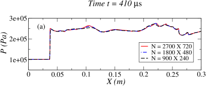
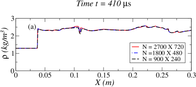
Figure 6: Pressure, (a) and density, (b) distributions for shock-He bubble interaction along the tube centre line at $t=410$ $\mu\rm{s}$ for different mesh resolutions.

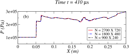
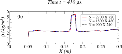
Figure 7: Pressure, (a) and density, (b) distributions for shock-Kr bubble interaction along the tube centre line at $t=410$ $\mu\rm{s}$ for different mesh resolutions

After performing numerical discretization tests, the experimental shadowgraph frames presented in Layes and Le Métayer (2007), were reproduced numerically. The computational simulations of the density field are presented by means of the idealized schlieren function at the same instants as in the experiment in Layes and Le Métayer (2007). Although the shapes of the deformed interfaces are recovered and can be observed clearly for different gas pairings it has to be noted that the accuracy of investigation is a function of experimental reproducibility. It is difficult to maintain the initial parameters of the shock wave Mach number, shape as well as size of the bubble and the gas composition from one to another experimental realisation Layes and Le Métayer (2007). For example the tolerance for $\textit{Ma}=1.5$ in the experiment was within the range: $1.45-1.52$. In spite of these difficulties the numerical results show a good approximation of the density contour plots obtained in the reference experiment.

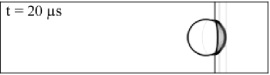
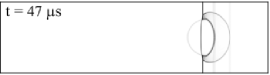
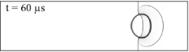
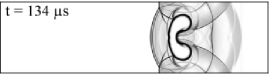
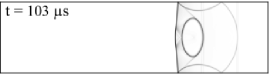
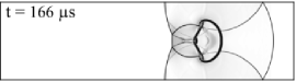
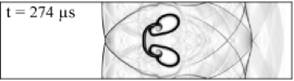
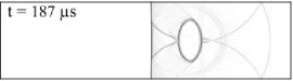
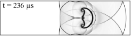
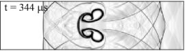
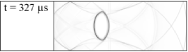
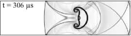
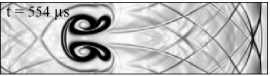
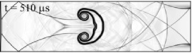
Figure 8: Numerical schlieren images showing the interface evolution in time of the different air/bubble constitutions: air/He (left), air/N₂ (middle) and air/Kr (right) at $\textit{Ma}=1.5$.

The positions of the characteristic interface points are recorded against time in Fig. 9. This figure also shows the changing positions of the incident and transmitted shock waves for air/He, air/N₂ and air/Kr configurations along the tube, which are measured from the shock initial position $X_{0}$, Fig. 5. The dynamic evolution of a bubble is observed by tracking points ($1$) and ($2$) originally placed on its contour, see Fig. 5. Point ($1$) is associated with the upstream front position and point ($2$) is the most downstream interface point. The usage of these tracking points to record numerically calculated spatial positions follows directly the experimental convention described in Layes and Le Métayer (2007). As it was earlier mention reproducible experiments with the same size of bubble were difficult to obtain. For example, the initial diameter of the nitrogen bubble in the experimental data is slightly larger than $4$ cm, Fig. 9(b2). Therefore the data from two realizations of the same experimental procedures presented in Layes and Le Métayer (2007), are utilized in the present comparison study. In spite of these difficulties the quantitative analysis of the computed positions in Fig. 9 shows excellent agreement with the experimental findings. The numerical results confirm the validity of the underlying governing equations and numerical method.

The first study presented in Fig. 9(a1, a2) shows the results for the helium bubble with lower acoustic impedance than the surrounding air. The difference in densities and therefore the higher sound speed in helium ($1007$ m/s) than in air ($340$ m/s) results in a higher speed for the transmitted shock through the helium bubble than for the incident shock in the air. The waves merge after passing the bubble to form a normal shock wave at around $270$ $\mu\rm{s}$ Fig. 9(a1). The early stages of the physical process reproduced numerically confirm the vorticity generation by the baroclinic effects. The rear interface of the helium bubble is caught by the front interface and the bubble evolves into a kidney shape. A penetrating high velocity jet along the flow direction moves through the bubble forming two symmetric flow configurations, Fig. 8. When the bubble deforms the associated flow field is subsequently split into two rings of vorticity. This characteristic separation further intensifies the deformation of the inhomogeneity.

The second study presented in Fig. 9(b1, b2) characterizes the interaction of a shock wave encountering a nitrogen bubble with comparable acoustic impedance as the surrounding air. The nitrogen and the air densities have similar values and therefore the corresponding Atwood number is close to zero. In such flow regime both the incident and the transmitted shock waves propagate with a small difference in velocities. After approximately $180$ $\mu\rm{s}$ the waves are combined again to form a planar shock wave. The generation and subsequent development of the vorticity field is negligible in this case. The compression process dominates the flow and the bubble evolution. The shape of the nitrogen bubble does not change significantly with time after around $200$ $\mu\rm{s}$ when the compression rate stabilizes.

The third study included in Fig. 9(c1, c2) reveals the numerical results for the krypton bubble. The krypton acoustic impedance is higher than the air acoustic impedance. Such situation makes the transmitted shock through the krypton bubble moving more slowly than the incident shock in the surrounding air. These waves fully converge after $300$ $\mu\rm{s}$. This case clearly shows that the vorticity drives the distortion mechanism. The shock passage generates vorticity on the bubble interface owing to misalignment of the pressure and density gradients across the interface. The vortical flow then distorts the bubble interface together with a penetrating jet that is generated after around $160$ $\mu\rm{s}$ along the symmetry line of the bubble which moves upstream towards the right hand side. In all these cases the different times at which shocks leave the tube were recorded. The accelerated shock in the helium case left the tube after around 480 $\mu\rm{s}$, in the nitrogen case the shock left the tube at around $500$ $\mu\rm{s}$ and finally, in the krypton case the shock was decelerated and left the tube after $510$ $\mu\rm{s}$.

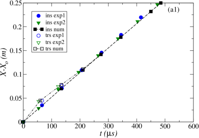
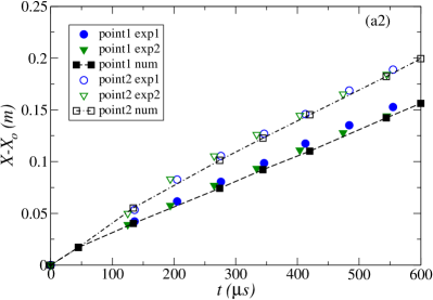
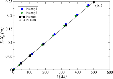
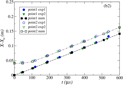
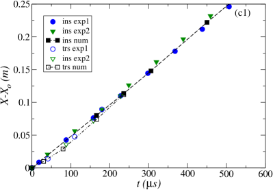
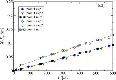
Figure 9: Incident shock (ins) and transmitted shock (trs) waves positions (left) and bubble points 1 and 2 locations (right) at $\textit{Ma}=1.5$ for air/He (a1, a2), air/N₂ (b1, b2) and air/Kr (c1, c2) constitutions. Comparison between present numerical results and experimental data Layes and Le Métayer (2007).

IV.2.2 Experiments of Zhai et al. Zhai et al. (2011)

The comparison study with both experimental and numerical results was carried out for the interaction of a weak $\textit{Ma}=1.2$ planar shock wave with a sulphur hexafluoride SF₆ bubble immersed in air. The Atwood number for this configuration is $A=0.66$. The advantage of the considered experiment over the previous investigations of Layes and Le Métayer (2007) is the application of a high speed schlieren photography with higher time resolution. This allows precise validations of the location of the wave front evolution both inside and outside the gas bubble at the very early stages of the interaction. As in Layes and Le Métayer (2007) the experiment was performed using a rectangular shock tube, Fig. 5, but with different dimensions of the observation window which were $0.07\times 0.5$ $\rm{m}$. The bubble initial diameter is $D_{0}=0.03~{}\rm{m}$ and the centre is located at a $0.02~{}\rm{m}$ distance from the shock. The numerical initial conditions are set per analogy to the previous investigation and are summarised in Table 5. The $2000\times 560$ computational grid provided a resolution of $240$ cells per bubble diameter. The CFL number was set to be equal to $0.3$.

Table 5: Initial conditions of the air/SF₆ shock-bubble interaction test

Physical property	SF6 bubble	pre-shocked air	post-shocked air
Density, $kg/m^{3}$	$5.97$	$1.19$	$1.597$
Horizontal velocity, $m/s$	$0.0$	$0.0$	$105.6$
Sound speed, $m/s$	$134$	$346$	$367$
Pressure, $Pa$	$101325$	$101325$	$153339$
Heat capacity ratio, $\gamma$	$1.1$	$1.4$	$1.4$
Acoustic impedance, $Pa\cdot s/m$	799.98	411.74	586.09

The schlieren images from the present simulation are collected in Fig. 10. The time interval between consecutive images is set to $10$ $\mu\rm{s}$ to capture the same sequences of the process as presented earlier in the experiment of Zhai et al. (2011). The images reveal the characteristic moments of the interaction and are in a very good agreement with the experimental and numerical results of Zhai et al. (2011). The images are numbered using the same convention as in the reference paper. The transmitted shock wave takes the convergent shape owing to the difference in acoustic impedance, Fig. 10 (images 1 to 5). Images 6 to 9, in the same figure, show two parts of the incident shock wave passing the top and the bottom poles of the bubble and moving towards the most downstream point of the interface. The transmitted shock starts to converge inside the bubble towards the centre of the downstream interface, Fig. 10 (images 10 to 13). As a result the formation of the penetrating jet can be observed in the following images. The process is driven by a high pressure zone resulting from the shock formation which concentrated at the downstream pole, Fig. 10 (images 14 and 15). This causes an explosion producing a refracted shock wave moving through the downstream boundary of the bubble from left to right and a shock wave propagating inside the bubble.

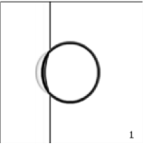
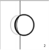
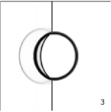
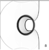
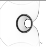
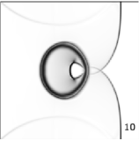
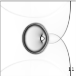
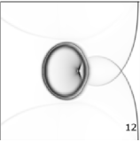
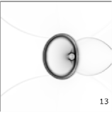
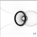
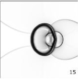
Figure 10: Sequence of schlieren images representing the SF₆ bubble evolution as a result of its interaction with a planar shock wave. The time interval between successive images from the numerical simulation is $10$ $\mu\rm{s}$.

The evolution is recorded using $x-t$ diagrams. Figure 11 defines the different tracking locations for the considered shock-bubble interaction reproduced in Fig. 10. The positions of the upstream interface (P1), downstream interface (P2), refracted (Rr), reflected (R1) and transmitted shock (Tr) are obtained at the horizontal axis while the incident shock (Ins) wave is measured at the undisturbed locations above the bubble.

Figure 12 refers to the distinct tracking points indicated in Fig. 11. The positions of these characteristic points, representing interface and various waves involved, are determined during the numerical simulation and their evolution is compared with (a) the experimental and (b) the numerical results reported in Zhai et al. (2011). The numerical predictions are in perfect agreement with the experimental data in the first stages of the interaction although a small difference in the position of the most downstream pole of the bubble is observed.

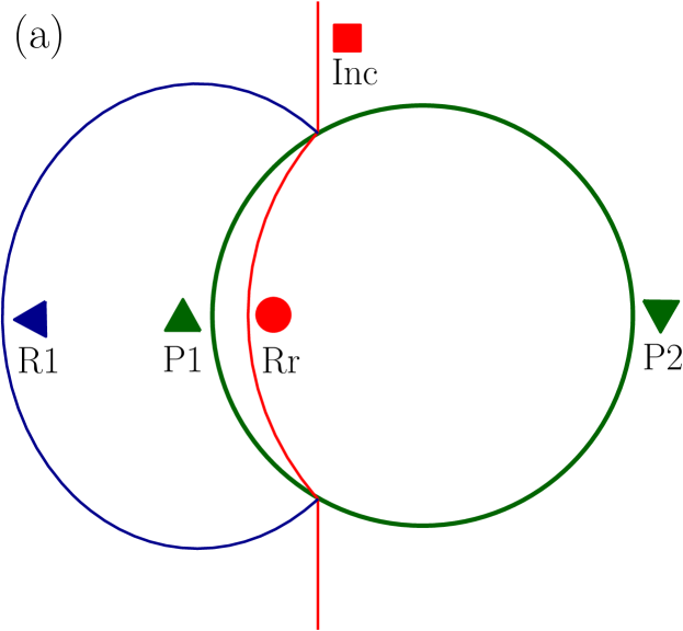
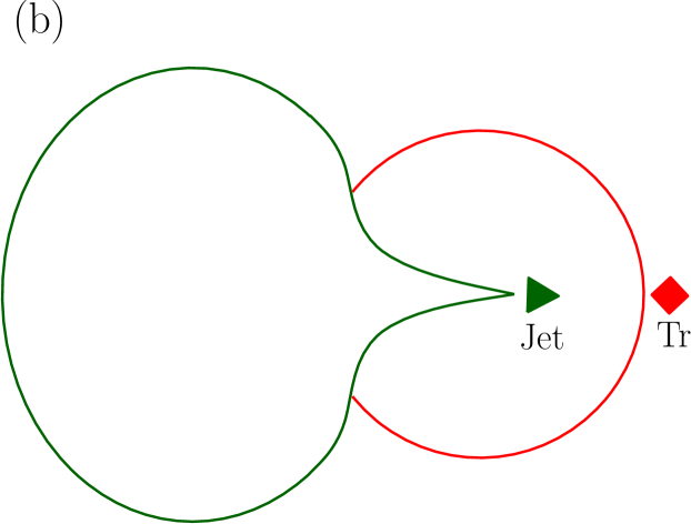
Figure 11: Schematic diagram with the characteristic elements of the interaction of a shock with a SF₆ bubble. Evolution stages: (a) early stage of the interaction (b) a moment after the shock wave passed the bubble. Tracking points: Inc-incident shock, P1-upstream interface, P2-downstream interface, R1-reflected shock, Rr-refracted shock, Tr-transmitted shock and Jet head

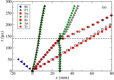
Figure 12: Recorded various shocks and interface positions during the interaction of a shock wave with a SF₆ bubble. Symbols are linked to the tracking locations shown in Fig. 11. The present numerical results (filled symbols) are compared with the experimental (a), and the numerical predictions (b) of Zhai et al. (2011).

Table 6 lists the velocities associated with the different shock waves. $V_{jet}$ is the velocity of the jet and $t_{jet}$ refers to the time at which the jet starts to form. Slight differences can be noticed between the numerical and experimental results. The main reason for these differences is due to the impurity of the gases inside and outside the bubble in the experiment which was acknowledged by Zhai et al. (2011).

Table 6: Comparison of the different velocities in the air/SF₆ shock bubble interaction test.

	Ma	$V_{inc}$	$V_{Rr}$	$V_{Rl}$	$V_{Tr}$	$V_{jet}$	$t_{jet}$
Experiment Zhai et al. (2011)	$1.2$	$395$	$203$	$347$	$488$	$114$	$140$
Computation Zhai et al. (2011)	$1.2$	$415$	$194$	$380$	$501$	$108$	$140$
Current computation	$1.2$	$410$	$197$	$380$	$501$	$108$	$140$

IV.3 Interface evolution and vorticity production as a function of Mach and Atwood numbers

After these successful validations the numerical procedures are applied to examine additional cases for which experimental data cannot be collected owing to the restrictions set by the physical apparatus. These new computational simulations consider the effect of a wider range of Atwood numbers on the shape of the interface as well as the effect of the Mach number on the interface growth and development. The influence of the Atwood and Mach number changes on the baroclinic source of the vorticity field is also investigated. Apart from the gases considered in the previous section the extra cases include the pairings of air/argon (Ar) with $A=0.13$. Therefore the numerical study accounts for the total of five different bubble/air configurations interacting with the waves for which Mach numbers were set to be 1.5, 2, 2.5 and 3. The initial data for these simulations are listed in Tables 7 and 8.

Table 7: Properties of the gas bubbles at atmospheric pressure and 15${}^{o}\rm{C}$.

Physical property	He	N2	Ar	Kr	SF6
Density, $kg/m^{3}$	0.169	1.19	1.67	3.55	6.27
Sound speed, $m/s$	1000	345	318	218	132
Heat capacity ratio $\gamma$	1.664	1.40	1.664	1.67	1.08
Acoustic impedance, $Pa\cdot s/m$	169	411	531	775	828

Table 8: Properties of air in the high pressure chamber.

Property	Case I	Case II	Case III	Case IV
Density, $kg/m^{3}$	2.242	3.211	4.013	4.644
Pressure, $Pa$	$2.49091\times 10^{5}$	$4.55963\times 10^{5}$	$7.21941\times 10^{5}$	$1.047025\times 10^{6}$
Mach number	1.5	2	2.5	3

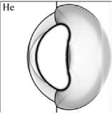
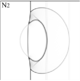
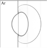
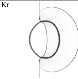
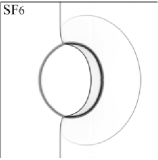
Figure 13: Numerical schlieren images for the various air/gas constitutions at time $60$ $\mu\rm{s}$ and $\textit{Ma}=1.5$.

Figure 14: Variation of the normalised transmitted shock velocity as a function of the Atwood number at time $60$ $\mu\rm{s}$ and $\textit{Ma}=1.5$.

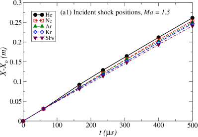
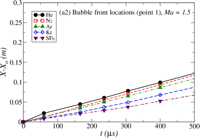
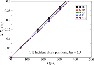
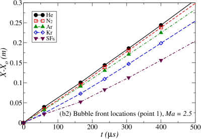
Figure 15: Incident shock and bubble upstream point 1 positions for different air/gas constitutions at $\textit{Ma}=1.5$ (a1, a2) and $\textit{Ma}=2.5$ (b1, b2).

Figure 13 shows the mixture density field profiles for different air/gas constitutions captured at the same early stage (60 $\mu\rm{s}$) of the bubble interactions with a shock wave of $\textit{Ma}=1.5$. The form of deformation of the bubble during the penetration of the shock wave is determined by the density and acoustic impedance of each constituent. The fastest speed of penetration was observed in the He bubble and this speed was at the same time faster than the normal incident shock. The situation was different in the cases of N₂ and Ar, where a slight difference between the speeds of transmitted and incident shock waves results in a smaller deformation of the bubble. The case of Kr and SF₆ exemplified a scenario opposite from that for He. In these cases the transmitted shock propagates through the bubbles more slowly than the incident shock outside the bubbles boundary. The transmitted shock in the SF₆ bubble moves also more slowly than in the Kr bubble. The early stages of the shock-bubble interaction in the last two cases did not allow for large deformations of the bubble. Figure 14 illustrates the relation between the velocity ratio ($U_{transmitted}/U_{incident}$) and the Atwood number at time $60$ $\mu\rm{s}$. It is observable that as the Atwood number goes towards positive values and becomes larger, the transmitted shock propagates through the bubble more slowly. Figure 15 shows the incident shock position and the location of the bubbles, filled with different gases, along the domain as a function of time for two different Mach numbers: $\textit{Ma}=1.5$ and $\textit{Ma}=2.5$. It is confirmed in Fig. 15(a1) and (b1) that the incident shock travels through the domain containing light bubbles faster than in the cases of heavy bubbles. The fact that the transmitted shock could accelerate or decelerate in the bubble environment has consequences at a later time, when the transmitted shock leaves the bubble and eventually combines with the incident shock. These are manifested by higher or lower wave speeds as compared to the medium containing a bubble with comparable physical properties to the surrounding medium or not containing a bubble at all. The location of the bubbles has been measured by tracking point ($1$) on the front of the bubble (upstream side, Fig. 5). The interpretation of Figs. 15(a2) and (b2) confirms that as the bubble is heavier it moves more slowly. Similarly these figures show the effect of the Mach number on the movement of the gas bubbles. The bubble covers a longer distance with higher Mach numbers. To assist in understanding the changes in the dynamics of the interface, the velocity values associated with point 1 on the upstream pole of the gas bubble were monitored. The values were collected for the Mach numbers $1.5$ and $2.5$, Fig. 16.

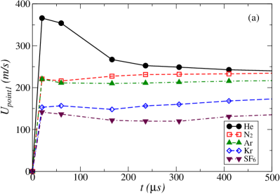
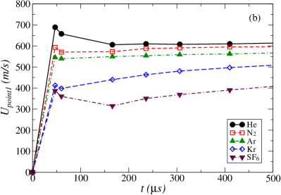
Figure 16: The velocities of point (1) for different gas bubbles as a function of time for (a) ${\it Ma}=1.5$ and (b) ${\it Ma}=2.5$.

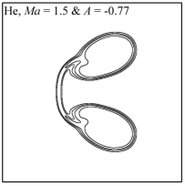
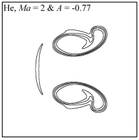
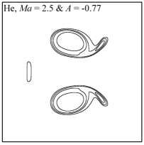
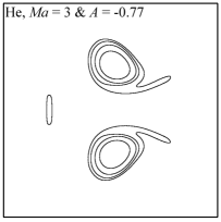
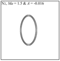
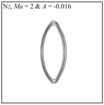
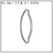
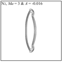
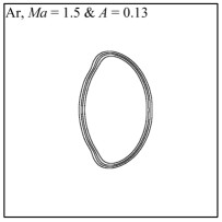
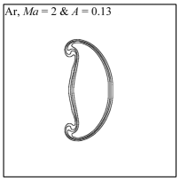
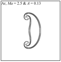
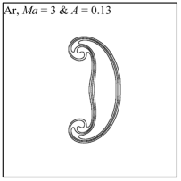
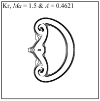
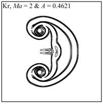
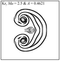
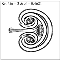
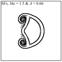
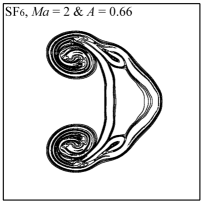
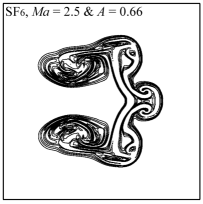
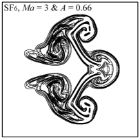
Figure 17: Volume fraction contours of various gas/air constitutions and Ma numbers at time 236 $\mu\rm{s}$.

Figure 18: Compression ratio of N₂ bubble as a function of the Mach number at time t = $510$ $\mu\rm{s}$.

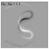
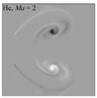
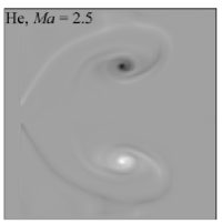
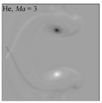
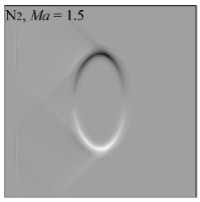
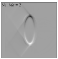
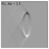
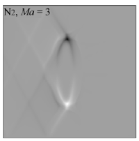
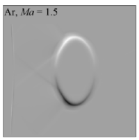
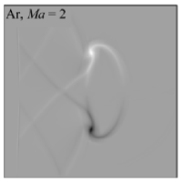
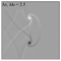
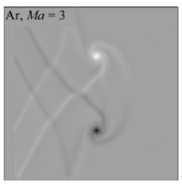
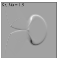
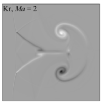
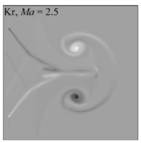
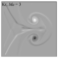
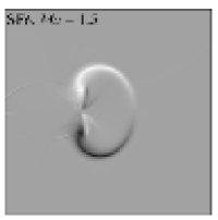
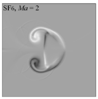
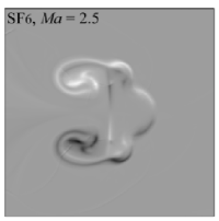
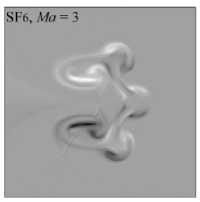
Figure 19: Vorticity field contours of various gas/air constitutions and Ma numbers at time $166~{}\mu\rm{s}$.

Figure 17 presents the evolutionary patterns of the interfaces represented by the volume fraction contours for various air/gas configurations and Mach numbers. The images are all taken at the same physical time equal to $236$ $\mu\rm{s}$ after the shock started to interact with the gas bubbles. Figure 17 can be read either from left to right (horizontal images - increase of Mach number) or from top to bottom (vertical images - increase of Atwood number). In the horizontal view one can see the effect of the Mach number on the interface evolution. The higher the Mach number the more changes in the interface shape, which is clearly seen in the last row of this horizontal view where the bubble undergoes distortion and consequently is divided into three entities with a significant interface evolution. In the case of the He bubble two symmetric contours can be observed as a result of the shock-bubble interaction. At the same time a high speed penetrating jet develops along the axis of symmetry in the main flow direction. The formation of the symmetric contours is more pronounced with the higher Mach numbers, leading eventually to a faster splitting of the bubble into two entities. A different situation is observed in case of the N₂ bubble. Here, the bubble is experiencing a compression process which intensifies with the higher Mach number. It is also found that the compression process happens at the early stages of the shock-bubble interactions allowing the bubble to stabilize its shape after around $200$ $\mu\rm{s}$ from the start of the interaction. This physical behaviour can be attributed to the fact that there is no penetrating jet or associated vorticity field (as the vorticity values are negligible in this case) which is clearly a direct consequence of the small density ratio of the constituents. Figure 18 illustrates the rate of compression of the N₂ bubble as a function of Mach number at the time $510$ $\mu\rm{s}$. The compression ratio increases with the Mach number and it is measured by dividing the horizontal diameter of the bubble ($D_{x}$) at time $510$ $\mu\rm{s}$ by the initial diameter ($D_{o}$). The Ar, Kr and SF₆ bubbles undergo a similar physical process until the moment when the baroclinic source of vorticity comes into play. This leads to greater bubble deformation and its interface distortion is even more apparent with the increasing Mach number. Another distinct feature of this process is the formation of the penetrating high speed jet along the bubble axis of symmetry, which moves in the opposite direction to the normal shock wave. The interface changes and jet development are clearer for a higher Atwood number Kr and SF₆ bubbles. The cases with the higher absolute value of the Atwood number experience a higher rate of the bubble deformation with increasing Mach numbers. In contrast, for the Atwood number close to zero the deformation rate of the interface is relatively slow.

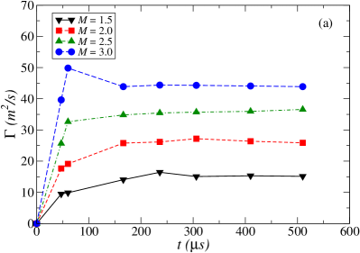
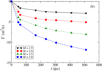
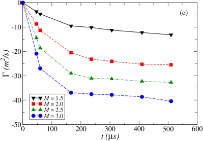
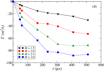
Figure 20: Time evolution of the circulation during the shock-bubble interaction process for different Mach numbers and gases: (a) air/He, (b) air/Ar, (c) air/Kr and (d) air/SF₆ constitutions.

Table 9: Circulation $\Gamma$(m²/s) at time t = $166$ $\mu\rm{s}$ for various flow constitutions and Ma numbers.

$Ma$	1.5	2.0	2.5	3.0
air/He	7.583	8.869	9.537	9.755
air/N2	0.184	0.096	0.097	0.113
air/Ar	$-1.820$	$-2.453$	$-2.621$	$-2.828$
air/Kr	$-5.709$	$-8.267$	$-8.986$	$-9.137$
air/SF6	$-11.649$	$-17.413$	$-23.209$	$-26.113$

Figure 19 shows the development of the vorticity field for all considered bubbles as a function of the Mach number. The snapshots were taken at the same time t = $166$ $\mu\rm{s}$. These pictures assist in the interpretation of the interface evolution process discussed previously, in which the vorticity creation plays an important role. To better understand Fig. 19, the vorticity field for different gases and Mach numbers is quantified by calculating the total circulation generated in the symmetrical half of the computational domain. The circulation values are listed in Table 9 for different Atwood and Mach numbers. The time evolutions of these values are presented in in Fig. 20. The shock propagates from the right to the left. Therefore in the case of light bubbles positive (anticlockwise) vortices are generated on the bottom side of the bubble and negative (clockwise) vortices are generated on the top side of the bubble. An opposite scenario is observed for the heavy bubbles, where vortices with positive sign are generated on the top and negative sign on the bottom of the bubbles. In later times (see especially the SF₆ evolution in Fig. 17), a dilation of the vorticity torus induced by its spiral effect can be observed. Looking at the values of the calculated circulation one can conclude that for the Atwood numbers of relatively high absolute values the vorticity generation rate becomes higher. When the Mach number is increased the value of the total circulation is also higher as its growth rate during the shock-bubble interaction process becomes faster. The effect of the vorticity on the N₂ bubble is negligible owing to the small differences in densities and acoustic impedance between N₂ and the surrounding air.

IV.4 Influence of the heat capacity ratio $(\gamma)$ on the bubble compression

In addition to the essential effect of the density ratio across the interfaces and the corresponding acoustic impedance difference, there is another fundamental parameter that contributes to the interface evolution. The heat capacity ratio $\gamma$ influences bubble compression and deformation. This parameter monitors how compressible the medium is. For example, SF₆ with $\gamma=1.08$ is much more compressible than the other mono and di-atomic gases, such as helium and nitrogen discussed in the previous section. In most of the literature concerned with the shock-bubble interaction problem, the analysis and discussions of this phenomenon is focused on the role of the acoustic impedance and the pressure misalignment on the interface deformation and vorticity production. The effect of $\gamma$ was not highlighted.

A new hypothetical shock-bubble interaction case study is designed to address the role of $\gamma$. This case study considers a planar shock of ${\it Ma}=1.5$ propagating in ambient air and interacting with an air bubble characterised by the same densities, i.e. zero Atwood number, but different values of $\gamma$. That is $\gamma=1.2,~{}1.4$ and $1.67$. The physical domain, Fig. 5, and computational set-up are the same as in subsection IV.2.1.

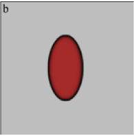
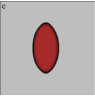
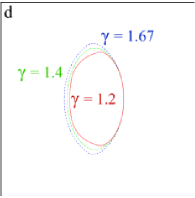
Figure 21: Volume fraction contours of the air bubbles at time $t=306~{}\mu{\rm s}$ for different interaction scenarios: (a) $\gamma=1.2$ (b) $\gamma=1.4$ (c) $\gamma=1.67$ and (d) comparison of volume fraction profiles.

Figures 21(a) to (c) show the volume fraction contours at the same physical time $306~{}\mu s$ from the beginning of the interaction for these three values of $\gamma$. The bubbles underwent a compression process as in the case of air/N₂ that was shown previously. However, the contour of each bubble has a slightly different shape. Figure 21(d) summarises the relative change of these different shapes of the bubbles with respect to $\gamma$. While for the case of $\gamma=1.2$ the bubble compresses more than the other two bubbles, the bubble with the largest gamma stretches vertically more than the others as shown in Fig. 20(d).

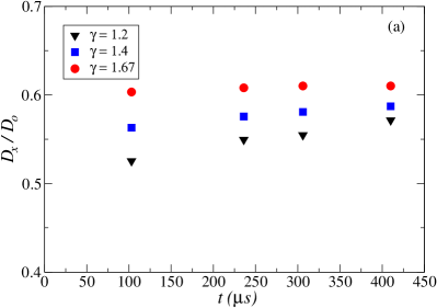
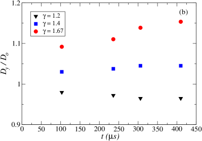
Figure 22: Relative change of the bubble size as a function of time (a) horizontal diameter (b) vertical diameter, during the interaction scenarios for different heat capacity ratios, $\gamma$.

Figure 22 quantifies the variation of the size of the bubbles along their horizontal and vertical diameters, with respect to time. $D_{0}$ is the initial diameter and $D_{x}$ and $D_{y}$ represent bubble horizontal and vertical diameters during the process of the shock-bubble interaction. The numerical results confirm that the heat capacity ratio $\gamma$ has an effect on the interface deformation. However, one has to remember that using this parameter separately in the discussion can be misleading. This is because the heat capacity ratio effects are already indirectly included in the acoustic impedance since the calculation of the sound speed of the gases across the interfaces requires $\gamma$.

The total circulation values recorded for various $\gamma$ are listed in Table 10. Although these values are negligible owing to small difference in acoustic impedance, they confirm the observations discussed in section IV.3.

Table 10: Circulation $\Gamma$(m²/s) as a function of time for various $\gamma$.

Time ($\mu s$)	$\gamma=1.2$	$\gamma=1.4$	$\gamma=1.67$
20	$-0.068$	0.000	0.080
47	$-0.163$	0.000	0.185
60	$-0.206$	0.000	0.233
103	$-0.268$	0.000	0.271

V Conclusions

The computations of flows in inhomogeneous media of various physical regimes leading to shock-bubble interactions were performed using a newly developed numerical code based on an Eulerian multi-component flow model. The numerical approach was validated using available data from shock tube experiments, for which very good qualitative and quantitative agreements were found. The present numerical approach could be applied to design better shock-induced mixing processes. In order to better understand the bubble shape changes and describe the mechanism of its interface deformation, the study was extended to include additional cases for which experimental data cannot be collected. These enabled us to account for the effect of the Atwood number and shock wave intensity (various Mach numbers) on the interface evolution and on the vorticity generation within the surrounding medium. The constant Mach number comparison showed that the Atwood number increase leads to higher vorticity generation and its effect on the interface evolution becomes more pronounced. Similarly the constant Atwood number comparison shows that increasing the Mach number produces a higher circulation which also means a higher vorticity generation. Apart from highlighting the cases characterised by the difference in acoustic impedance the study was extended to account for the influence of the heat capacity ratio $\gamma$ of the heterogeneous media on the interface deformation. The results of this study, which could potentially constitute a benchmark test for other numerical simulations, confirm that the baroclinic term in the vorticity transport equation has a large effect on the interface evolution and the vorticity generation. The 2D simulations can only be used as a platform for the analysis of early stages of a shock wave-spherical bubble interaction. For longer time periods after a planar shock-inhomogeneity interaction, the flow becomes 3D and vorticity structures are influenced by vortex stretching.

References

- Aglitskiy et al. (2010) Y. Aglitskiy, A.L. Velikovich, M. Karasik, N. Metzler, S.T. Zalesak, A.J. Schmitt, L. Phillips, J.H. Gardner, V. Serlin, J.L. Weaver, and S.P. Obenschain, “Basic hydrodynamics of Richtmyer-Meshkov-type growth and oscillations in the inertial confinement fusion-relevant conditions,” Phil. Trans. R. Soc. A 368, 1739–1768 (2010).
- Ranjan et al. (2011) D. Ranjan, J. Oakley, and R. Bonazza, “Shock-bubble interactions,” Annu. Rev. Fluid Mech. 43, 117–140 (2011).
- Brouillette (2002) M. Brouillette, “The Richtmyer-Meshkov instability,” Annu. Rev. Fluid Mech. 34, 445–468 (2002).
- Haas and Sturtevant (1987) J.F. Haas and B. Sturtevant, “Interaction of weak shock waves with cylindrical and spherical gas inhomogeneities,” J. Fluid Mech. 181, 41–76 (1987).
- Layes et al. (2003) G. Layes, G. Jourdan, and L. Houas, “Distortion of a spherical gaseous interface accelerated by a plane shock wave,” Phys. Rev. Lett. 91, 174502 (2003).
- Layes and Le Métayer (2007) G. Layes and O. Le Métayer, “Quantitative numerical and experimental studies of the shock accelerated heterogeneous bubbles motion,” Phys. Fluids 19, 042105 (2007).
- Layes et al. (2009) G. Layes, G. Jourdan, and L. Houas, “Experimental study on a plane shock wave accelerating a gas bubble,” Phys. Fluids 21, 074102 (2009).
- Zhai et al. (2011) Z. Zhai, T. Si, X. Luo, and J. Yang, “On the evolution of spherical gas interfaces accelerated by a planar shock wave,” Phys. Fluids 23, 084104 (2011).
- Si et al. (2012) T. Si, Z. Zhai, J. Yang, and X. Luo, “Experimental investigation of reshocked spherical gas interfaces,” Phys. Fluids 24, 054101 (2012).
- Ranjan et al. (2007) D. Ranjan, J. Niederhaus, B. Motl, M. Anderson, J. Oakley, and R. Bonazza, “Experimental investigation of primary and secondary features in high-Mach-number shock-bubble interaction,” Phys. Rev. Lett. 98 (2007).
- Ranjan et al. (2008) D. Ranjan, J.H.J. Niederhaus, J.G. Oakley, M.H. Anderson, J.A. Greenough, and R. Bonazza, “Experimental and numerical investigation of shock-induced distortion of a spherical gas inhomogeneity,” Phys. Scripta T132, 014020 (2008).
- Haehn et al. (2012) N. Haehn, C. Weber, J. Oakley, M. Anderson, D. Ranjan, and R. Bonazza, “Experimental study of the shock-bubble interaction with reshock,” Shock Waves 22, 47–56 (2012).
- Tomkins et al. (2008) C. Tomkins, S. Kumar, G. Orlicz, and K. Prestridge, “An experimental investigation of mixing mechanisms in shock-accelerated flow,” J. Fluid Mech. 611, 131–150 (2008).
- Zabusky and Zeng (1998) N.J. Zabusky and S.M. Zeng, “Shock cavity implosion morphologies and vortical projectile generation in axisymmetric shock spherical fast/slow bubble interactions,” J. Fluid Mech. 362, 327–346 (1998).
- Picone and Boris (1988) J.M. Picone and J.P. Boris, “Vorticity generation by shock propagation through bubbles in a gas,” J. Fluid Mech. 189, 23–51 (1988).
- Quirk and Karni (1996) J.J. Quirk and S. Karni, “On the dynamics of a shock-bubble interaction,” J. Fluid Mech. 318, 129–163 (1996).
- Bagabir and Drikakis (2001) A. Bagabir and D. Drikakis, “Mach number effects on shock-bubble interaction,” Shock Waves 11, 209–218 (2001).
- Banks et al. (2007) J.W. Banks, D.W. Schwendeman, A.K. Kapila, and W.D. Henshaw, “A high-resolution Godunov method for compressible multi-material flow on overlapping grids,” J. Comput. Phys. 223, 262–297 (2007).
- Chang and Liou (2007) C.-H. Chang and M.-S. Liou, “A robust and accurate approach to computing compressible multiphase flow: Stratified flow model and AUSM+-up scheme,” J. Comput. Phys. 225, 840–873 (2007).
- Terashima and Tryggvason (2009) H. Terashima and G. Tryggvason, “A front-tracking/ghost-fluid method for fluid interfaces in compressible flows,” J. Comput. Phys. 288, 4012–4037 (2009).
- Hejazialhosseini et al. (2010) B. Hejazialhosseini, D. Rossinelli, M. Bergdorf, and P. Koumoutsakos, “High order finite volume methods on wavelet-adapted grids with local time-stepping on multicore architectures for the simulation of shock-bubble interactions,” J. Comput. Phys. 229, 8364–8383 (2010).
- Shukla et al. (2010) R.K. Shukla, C. Pantano, and J.B. Freund, “An interface capturing method for the simulation of multi-phase compressible flows,” J. Comput. Phys. 229, 7411–7439 (2010).
- So et al. (2012) K.K. So, X.Y. Hu, and N.A. Adams, “Anti-diffusion interface sharpening technique for two-phase compressible flow simulations,” J. Comput. Phys. 231, 4304–4323 (2012).
- Franquet and Perrier (2012) E. Franquet and V. Perrier, “Runge-Kutta discontinuous Galerkin method for the approximation of Baer and Nunziato type multiphase models,” J. Comput. Phys. 231, 4096–4141 (2012).
- Niederhaus et al. (2008) J. Niederhaus, J. Greenough, J. Oakley, D. Ranjan, M. Anderson, and R. Bonazza, “A computational parameter study for the three-dimensional shock-bubble interaction,” J. Fluid Mech. 594, 85– 124 (2008).
- Giordano and Burtschell (2006) J. Giordano and Y. Burtschell, “Richtmyer-Meshkov instability induced by shock-bubble interaction: Numerical and analytical studies with experimental validation,” Phys. Fluids 18, 036102 (2006).
- Baer and Nunziato (1986) M.R. Baer and J.W. Nunziato, “A two-phase mixture theory for the deflagration-to-detonation transition(DDT) in reactive granular materials,” Int. J. Multiphase Flow 12, 861–889 (1986).
- Kapila et al. (2001) A.K. Kapila, R. Menikoff, J.B. Bdzil, S.F. Son, and D.S. Stewart, “Two-phase modeling of deflagration to detonation transition in granular materials: Reduced equations,” Phys. Fluids 13, 3002–3024 (2001).
- Saurel et al. (2009) R. Saurel, F. Petitpas, and R.A. Berry, “Simple and efficient relaxation methods for interfaces separating compressible fluids, cavitating flows and shocks in multiphase mixtures,” J. Comput. Phys. 228, 1678–1712 (2009).
- Murrone and Guillard (2005) A. Murrone and H. Guillard, “A five-equation reduced model for compressible two phase flow problems,” J. Comput. Phys. 202, 664–698 (2005).
- Godunov (2008) S.K. Godunov, “On approximations for overdetermined hyperbolic equations,” in Hyperbolic Problems: Theory, Numerics, Applications, edited by S. Benzoni-Gavage and D. Serre (Springer Berlin Heidelberg, 2008) pp. 19–33.
- Schilling et al. (2007) O. Schilling, M. Latini, and W.S. Don, “Physics of reshock and mixing in single-mode Richtmyer-Meshkov instability,” Phys. Rev. E 76, 026319 (2007).
- Toro (1999) E. Toro, Riemann Solvers and Numerical Methods for Fluid Dynamics (Springer, 1999).
- Harten et al. (1983) A. Harten, Peter D. Lax, and Bram Van Leer, “On upstream differencing and Godunov-type schemes for hyperbolic conservation laws,” SIAM Rev. 25, 35–61 (1983).
- Lallemand et al. (2005) M.H. Lallemand, A. Chinnayya, and O. Le Metayer, “Pressure relaxation procedures for multiphase compressible flows,” Int. J. Numer. Meth. Fluids. 49, 1–56 (2005).
- Strang (1968) G. Strang, “On the construction and comparison of difference schemes,” SIAM J. Numer. Anal 5, 506–517 (1968).
- Henderson (1966) L.F. Henderson, “The refraction of a plane shock wave at a gas interface,” J. Fluid Mech. 26, 607–637 (1966).
- Henderson (1989) L.F. Henderson, “On the refraction of shock waves,” J. Fluid Mech. 198, 365–386 (1989).
- Hejazialhosseini et al. (2013) B. Hejazialhosseini, D. Rossinelli, and P. Koumoutsakos, “Vortex dynamics in 3D shock-bubble interaction,” Phys. Fluids 25, 110816 (2013).
- Kevlahan (1997) N.K.-R. Kevlahan, “The vorticity jump across a shock in a non-uniform flow,” J. Fluid Mech. 341, 371–384 (1997).
- Huete et al. (2011) C. Huete, A.L. Velikovich, and J.G. Wouchuk, “Analytical linear theory for the interaction of a planar shock wave with a two- or three-dimensional random isotropic density field,” Phys. Rev. E 83, 056320 (2011).
- Huete et al. (2012) C. Huete, J.G. Wouchuk, and A.L. Velikovich, “Analytical linear theory for the interaction of a planar shock wave with a two- or three-dimensional random isotropic acoustic wave field,” Phys. Rev. E 85, 026312 (2012).
- Wouchuk and Sano (2015) J.G. Wouchuk and T. Sano, “Normal velocity freeze-out of the Richtmyer-Meshkov instability when a rarefaction is reflected,” Phys. Rev. E 91, 023005 (2015).
- Abgrall and Saurel (2003) R. Abgrall and R. Saurel, “Discrete equations for physical and numerical compressible multiphase mixtures,” J. Comput. Phys. 186, 361–396 (2003).
- Sun and Takayama (1999) M. Sun and K. Takayama, “Conservative smoothing on an adaptive quadrilateral grid,” J. Comput. Phys. 150, 143–180 (1999).