LRS Bianchi type-I cosmological model with constant deceleration parameter in $f(R,T)$ gravity

Abstract

A spatially homogeneous anisotropic LRS Bianchi type-I cosmological model is studied in $f(R,T)$ gravity with a special form of Hubble’s parameter, which leads to constant deceleration parameter. The parameters involved in the considered form of Hubble parameter can be tuned to match, our models with the $\Lambda$CDM model. With the present observed value of the deceleration parameter, we have discussed physical and kinematical properties of a specific model. Moreover, we have discussed the cosmological distances for our model.

Mathematics Subject Classification 2010: 83F05, 83C15

1 Introduction

Observation plays a major role in modern cosmology. The advent of new technologies in observations enforces the theorists to rethink on the formulation of the gravitational theories time to time. Einstein had to drop the cosmological constant from the field equations with the discovery of Hubble. The concept of decelerating expansion of the Universe had to drop by the theorists with the observation of type Ia supernovae in 1998. Since then CMB, BAO, SDSS and many more observations provide evidences in support of the accelerating expansion of the Universe. So, it is very important to take care of the observational results while building a theoretical model of the Universe. The accelerating expansion of the Universe is an important feature of present day cosmology. The Einstein field equations (EFEs) always lead to a decelerating expansion with the normal matter component in the Universe. The accelerating expansion can be described either by supplying some extra component in the energy momentum tensor part in the field equations or by doing some modifications in the geometrical part. With these principles, the past few years of research produced a plethora of cosmological models of the Universe explaining the accelerating expansion. The theory of dark energy have taken special status in recent times. The dark energy is an exotic energy component with negative pressure, which explain many observations well and solves some major problems of standard cosmology. The second possibility is by assuming that the general relativity breaks down at large scales and the gravitational field can be described by a more general action.

The $f(R)$ theory of gravity [1, 2, 3, 4, 5, 6, 7] is an alternative to General Relativity (GR) to justify the cosmic acceleration and early inflation in different way. In $f(R)$ theory, the cosmic acceleration is obtained by the term $\frac{1}{R}$ where $R$ is the Ricci scalar in the Einstein-Hilbert action. $f(R)$ gravity models also addressed the issue of dark matter [8, 9, 10, 11]. Recently, the mimetic $F(R)$ gravity [12, 13, 14] has been proposed to investigate the early-time and late-time acceleration of the universe. It is demonstrated that the mimetic $F(R)$ gravity consistent with Plank and BICEP2/Keck Array observations. The $f(R)$ gravity was modified by introducing the trace of energy momentum tensor $T$ to the action yielding $f(R,T)$ gravity [15]. The action for the $f(R,T)$ gravity is given as

$$S=\int\sqrt{-g}\left(\frac{f(R,T)}{16\pi}+L_{m}\right)d^{4}x$$ (1)

where $L_{m}$ is the matter Lagrangian and $g=|g_{ij}|$. Varying the action in equation (1) with respect to metric tensor $g_{ij}$ the field equations are obtained as

$$f_{R}(R,T)R_{ij}-\frac{1}{2}f(R,T)g_{ij}+(g_{ij}\Box-\nabla_{i}\nabla_{j})f_{R}(R,T)=\\ 8\pi T_{ij}-f_{T}(R,T)T_{ij}-f_{T}(R,T)\Theta_{ij}$$ (2)

where

$$\Theta_{ij}=-2T_{ij}+g_{ij}L_{m}-2g^{lm}\frac{\partial^{2}L_{m}}{\partial g^{ij}\partial g^{lm}}$$ (3)

Here $f_{R}(R,T)=\frac{\partial f(R,T)}{\partial R}$, $f_{T}(R,T)=\frac{\partial f(R,T)}{\partial T}$, $\Box\equiv\nabla^{i}\nabla_{i}$ where $\nabla_{i}$ represents covariant derivative.
Contraction of equation (3) yields

$$f_{R}(R,T)R+3\Box f_{R}(R,T)-2f(R,T)=(8\pi-f_{T}(R,T))T-f_{T}(R,T)\Theta$$ (4)

where $\Theta=g^{ij}\Theta_{ij}$. From equations (2) and (4), one can obtain

$$f_{R}(R,T)\biggl{(}R_{ij}-\frac{1}{3}Rg_{ij}\biggr{)}+\frac{1}{6}f(R,T)g_{ij}=\\ 8\pi-f_{T}(R,T)\biggl{(}T_{ij}-\frac{1}{3}Tg_{ij}\biggr{)}-f_{T}(R,T)\biggl{(}\Theta_{ij}-\frac{1}{3}\Theta g_{ij}\biggr{)}+\nabla_{i}\nabla_{j}f_{R}(R,T)\text{.}$$ (5)

Numerous works have been done in the past few years in $f(R,T)$ theory of gravity due to the growing interests on the modified theories. One can see a recent work for a case study on $f(R,T)$ gravity in Salehi and Aftabi [16]. Hundjo et al. [17] has developed the cosmological reconstruction of $f(R,T)$ gravity and discussed the transition of matter dominated phase to an accelerated phase. The non-equilibrium picture of thermodynamics at apparent horizon for Friedmann-Robertson-Walker (FRW) universe is discussed in this theory [18]. Sharif et al. [19] have studied various energy conditions in $f(R,T)$ gravity and they reduce the same to $f(R)$ and $f(T)$ gravity. The Godel solutions are derived in this modified theory [20, 21]. Memoni et al. [22] have studied the generalized second law of thermodynamics in $f(R,T)$ gravity. The effect of bulk viscosity in $f(R,T)$ gravity is discussed for FRW metric [23]. Shri Ram and Chandel [24] have discussed dynamics of magnetized string cosmological model. Two classes of $f(R,T)$ gravity models is investigated by Shamir and Raja [25] for cylindrically symmetric space-time. Mores et al. [26] have discussed about the hydro static equilibrium configuration of neutron stars and strange stars in the contexts of $f(R,T)$ gravity. Here the fluid pressure is computed from the equations of state (EoS) $\rho=\omega\rho^{\frac{5}{3}}$ and $p=0.28(\rho-4B)$, where $B$ is a constant and $\rho$ is the energy density of the fluid. Alhamzawi and Alhamzawi [27] have discussed the gravitational lensing in first class of $f(R,T)$ gravity. They have calculated the effect of $f(R,T)$ gravity on gravitational lensing and shown that it can give a considerable contribution to gravitational lensing. Mores [28] has discussed the varying speed of light in $f(R,T)$ gravity. Alves et al. [29] have studied the gravitational waves scenario in this theory. Yousaf et al [30] have investigated the irregularity factor of self gravitating star due to imperfect fluid in $f(R,T)$ gravity.

Though the observations is in favour of a homogeneous and isotropic Universe, the possibility of anisotropic phase in the early Universe is also supported by some observations. Also the presence of anisotropy affect the evolution of energy density. Evolution of anisotropic source for axially symmetric universe have been discussed in $f(R,T)$ gravity [31]. The dynamical analysis of anisotropic spherically symmetric collapsing star has presented in this modified gravity [32]. This motivates the theorists to construct various models in different Bianchi space-times in different contexts [33, 34, 35, 36, 37, 38]. In this paper, we consider LRS Bianchi-I space-time as our background metric and study the evolution of various cosmological parameters in $f(R,T)$ theory of gravity.

2 Metric and Field Equations for $f(R,T)=f_{1}(R)+f_{2}(T)$

The spatially homogeneous anisotropic LRS Bianchi type-I metric

$$ds^{2}=dt^{2}-A(t)^{2}(dx^{2}+dy^{2})-B(t)^{2}dz^{2}\text{,}$$ (6)

is symmetric corresponding to $xy-$plane. The average scale factor $a$, spatial volume $V$, scalar expansion $\theta$ for metric (6) are

$$a=(A^{2}B)^{\frac{1}{3}},\ \ V=a^{3}=A^{2}B,\ \ \theta=u_{;i}^{i}=2\frac{A^{\prime}}{A}+\frac{B^{\prime}}{B}\text{.}$$ (7)

For $f(R,T)=f_{1}(R)+f_{2}(T)$, we consider the linear form $f_{1}(R)=\lambda R$ and $f_{2}(T)=\lambda T$ where $\lambda$ is an arbitrary constant. Hence, in this case $f(R,T)=\lambda(R+T)$. We considered the source of matter as perfect fluid having energy momentum tensor

$$T_{ij}=(\rho+p)u_{i}u_{j}-pg_{ij}$$ (8)

where $u^{i}=(0,0,0,1)$ is four velocity vector satisfying $u^{i}u_{i}=1$, the $f(R,T)$ gravity field equations (5) takes the form

$$\lambda R_{ij}-\frac{1}{2}\lambda(R+T)g_{ij}+(g_{ij}\Box-\nabla_{i}\nabla_{j})\lambda=8\pi T_{ij}-\lambda T_{ij}+\lambda(2T_{ij}+pg_{ij})\text{.}$$ (9)

Since $(g_{ij}\Box-\nabla_{i}\nabla_{j})\lambda=0$, we obtain

$$R_{ij}-\frac{1}{2}Rg_{ij}=\biggl{(}\frac{8\pi+\lambda}{\lambda}\biggr{)}T_{ij}+\biggl{(}p+\frac{1}{2}T\biggr{)}g_{ij}\text{ .}$$ (10)

From GR the Einstein tensor $G_{ij}\equiv R_{ij}-\frac{1}{2}g_{ij}R$. Using this in equation (10), we can write

$$G_{ij}-\biggl{(}p+\frac{1}{2}T\biggr{)}g_{ij}=\biggl{(}\frac{8\pi+\lambda}{\lambda}\biggr{)}T_{ij}.$$ (11)

In GR, the field equations with cosmological constant $\Lambda$ usually written as

$$G_{ij}-\Lambda g_{ij}=-8\pi T_{ij}\text{ .}$$ (12)

Here, we assume a small $-$ve value for $\lambda$ throughout the manuscript to get a better analogy with usual Einstein field equations.
Comparison of (11) and (12) gives us

$$\Lambda\equiv\Lambda(T)=p+\frac{1}{2}T\text{,}$$ (13)

and $\lambda=-\frac{8\pi}{8\pi+1}$. In other words, $p+\frac{1}{2}T$ behaves as cosmological constant. The field equations (10), for the metric (6) can be obtained as

$$\frac{A^{\prime\prime}}{A}+\frac{A^{\prime}B^{\prime}}{AB}+\frac{B^{\prime\prime}}{B}=\biggl{(}\frac{8\pi+\lambda}{\lambda}\biggr{)}p-\Lambda\text{,}$$ (14)

$$2\frac{A^{\prime\prime}}{A}+\biggl{(}\frac{A^{\prime}}{A}\biggr{)}^{2}=\biggl{(}\frac{8\pi+\lambda}{\lambda}\biggr{)}p-\Lambda\text{,}$$ (15)

$$\biggl{(}\frac{A^{\prime}}{A}\biggr{)}^{2}+2\frac{A^{\prime}B^{\prime}}{AB}=-\biggl{(}\frac{8\pi+\lambda}{\lambda}\biggr{)}\rho-\Lambda\text{,}$$ (16)

where an overhead prime denote derivative with respect to time ‘$t$’ only. The trace $T$ for this model is $T=-3p+\rho$, so that equation (13) reduces to

$$\Lambda(T)=\frac{1}{2}(\rho-p)\text{.}$$ (17)

From equations (14) and (15), we have

$$\frac{A^{\prime}}{A}-\frac{B^{\prime}}{B}=\frac{c_{1}}{A^{2}B}\text{,}$$ (18)

where $c_{1}$ is constant of integration. Again integrating

$$\frac{A}{B}=c_{2}\exp\biggl{[}c_{1}\int\frac{dt}{A^{2}B}\biggr{]}=c_{2}\exp\biggl{[}c_{1}\int\frac{dt}{a^{3}}\biggr{]}\text{,}$$ (19)

where $c_{2}$ is integration constant.
Using the above value in equation (7), we can get

$$A=c_{2}^{1/3}a\exp\biggl{[}\frac{c_{1}}{3}\int\frac{dt}{a^{3}}\biggr{]}$$ (20)

and

$$B=c_{2}^{-2/3}a\exp\biggl{[}\frac{-2c_{1}}{3}\int\frac{dt}{a^{3}}\biggr{]}\text{.}$$ (21)

The directional Hubble parameters are defined as $H_{1}=\frac{A^{\prime}}{A}$ and $H_{2}=\frac{B^{\prime}}{B}$ comes out as $H=\frac{1}{3}(2H_{1}+H_{2})$ and $\theta=3H$. The shear scalar $\sigma^{2}$ for the metric (6) is written as

$$\sigma^{2}=\frac{1}{2}\biggl{[}\sum H_{i}^{2}-\frac{1}{3}\theta^{2}\biggr{]}=\frac{1}{3}(H_{1}-H_{2})^{2}\text{.}$$ (22)

Using directional Hubble parameters, we can write the field equations (14)-(16) as

$$H_{1}^{\prime}+H_{2}^{\prime}+H_{1}^{2}+H_{2}^{2}+H_{1}H_{2}=\alpha p-\Lambda\text{,}$$ (23)

$$2H_{1}^{\prime}+3H_{1}^{2}=\alpha p-\Lambda\text{,}$$ (24)

$$H_{1}^{2}+H_{1}H_{2}=-\alpha\rho-\Lambda\text{,}$$ (25)

where $\alpha=\frac{8\pi+\lambda}{\lambda}$. The Ricci scalar $R$ for our model is

$$R=-2\biggl{[}2\frac{A^{\prime\prime}}{A}+2\frac{A^{\prime}B^{\prime}}{AB}+\frac{B^{\prime\prime}}{B}+\biggl{(}\frac{A^{\prime}}{A}\biggr{)}^{2}\biggr{]}$$ (26)

Pressure, energy density and the cosmological constant for the model can be written in terms of Hubble parameter as

$$p=\frac{(4\alpha+2)H_{1}^{\prime}+(6\alpha+2)H_{1}^{2}-H_{1}H_{2}}{2\alpha(\alpha+1)}$$ (27)

$$\rho=\frac{2H_{1}^{\prime}+(2-2\alpha)H_{1}^{2}-(2\alpha+1)H_{1}H_{2}}{2\alpha(\alpha+1)}$$ (28)

$$\Lambda=-\frac{2H_{1}^{\prime}+4H_{1}^{2}+H_{1}H_{2}}{2(\alpha+1)}$$ (29)

The equation of state parameter i.e. the ratio between pressure and energy density is

$$\omega=\frac{(4\alpha+2)H_{1}^{\prime}+(6\alpha+2)H_{1}^{2}-H_{1}H_{2}}{2H_{1}^{\prime}+(2-2\alpha)H_{1}^{2}-(2\alpha+1)H_{1}H_{2}}$$ (30)

Having a general set up, we look for solutions to the field equations in the next section.

3 Solution of the Field Equations

In order to obtain an explicit solutions to the field equations, we require a supplementary constrain equation for the consistency of the system. This one extra constrain can be chosen by assuming linear relationship between two variables in the field equations or we can parametrize any particular variable. For a recent review on various parametrization one can see [39]. Recently Pacif and Mishra [40] have proposed special law of variation of Hubble parameter

$$H=\frac{m}{k_{1}t+k_{2}},$$ (31)

where $m\geq 0$, $k_{1}\neq 0$ and $k_{2}$ are constants and this readily gives the scale factor explicitly as

$$a(t)=k_{3}(k_{1}t+k_{2})^{\frac{m}{k_{1}}}\text{,}$$ (32)

where $k_{3}$ is integration constant. The deceleration parameter $q$ comes out to be a constant depending on $k_{1}$and $m$.

$$q=-1+\frac{d}{dt}\left(\frac{1}{H}\right)=-1+\frac{k_{1}}{m}\text{.}$$ (33)

Using the equation (32) in (20) and (21) the metric potentials are obtained as functions of time as

$$A=c_{2}^{\frac{1}{3}}k_{3}(k_{1}t+k_{2})^{\frac{m}{k_{1}}}\times\exp\left[\frac{c_{1}(k_{1}t+k_{2})^{1-\frac{3m}{k_{1}}}}{3k_{3}^{3}(k_{1}-3m)}\right]$$ (34)

$$B=c_{2}^{\frac{-2}{3}}k_{3}(k_{1}t+k_{2})^{\frac{m}{k_{1}}}\times\exp\left[\frac{-2c_{1}(k_{1}t+k_{2})^{1-\frac{3m}{k_{1}}}}{3k_{3}^{3}(k_{1}-3m)}\right]$$ (35)

The directional Hubble parameters $H_{1}$ and $H_{2}$ becomes

$$H_{1}=\frac{c_{1}(k_{1}t+k_{2})^{-\frac{3m}{k_{1}}}}{3k_{3}^{3}}+\frac{m}{k_{1}t+k_{2}}$$ (36)

$$H_{2}=\frac{(k_{1}t+k_{2})^{-\frac{3m}{k_{1}}-1}\left(3k_{3}^{3}m(k_{1}t+k_{2})^{\frac{3m}{k_{1}}}-2c_{1}(k_{1}t+k_{2})\right)}{3k_{3}^{3}}$$ (37)

The expansion scalar $\theta$ and the shear $\sigma^{2}$ are obtained as

$$\theta=3H=\frac{3m}{k_{1}t+k_{2}},\ \ \ \sigma^{2}=\frac{c_{1}^{2}(k_{1}t+k_{2})^{-\frac{6m}{k_{1}}}}{3k_{3}^{6}}$$ (38)

The anisotropy parameter $\Delta$ of the expansion is

$$\Delta=6\left(\frac{\sigma}{\theta}\right)^{2}=\frac{2c_{1}^{4}(k_{1}t+k_{2})^{2-\frac{12m}{k_{1}}}}{27k_{3}^{12}m^{2}}$$ (39)

The other dynamical parameters for our model are obtained as

$$p=\frac{(k_{1}t+k_{2})^{-\frac{6m}{k_{1}}-2}\left(\begin{array}[]{c}2(3\alpha+2)c_{1}^{2}(k_{1}t+k_{2})^{2}-3c_{1}k_{3}^{3}m(k_{1}t+k_{2})^{\frac{3m}{k_{1}}+1}\\ +9k_{3}^{6}m(-2(2\alpha+1)k_{1}+6\alpha m+m)(k_{1}t+k_{2})^{\frac{6m}{k_{1}}}\end{array}\right)}{18\alpha(\alpha+1)k_{3}^{6}}$$ (40)

$$\rho=\frac{(k_{1}t+k_{2})^{-\frac{6m}{k_{1}}-2}\left(\begin{array}[]{c}2(\alpha+2)c_{1}^{2}(k_{1}t+k_{2})^{2}-3(2\alpha+1)c_{1}k_{3}^{3}m(k_{1}t+k_{2})^{\frac{3m}{k_{1}}+1}\\ -9k_{3}^{6}m(2k_{1}+(4\alpha-1)m)(k_{1}t+k_{2})^{\frac{6m}{k_{1}}}\end{array}\right)}{18\alpha(\alpha+1)k_{3}^{6}}$$ (41)

$$\Lambda=\frac{(k_{1}t+k_{2})^{-\frac{6m}{k_{1}}-2}\left(\begin{array}[]{c}-2c_{1}^{2}(k_{1}t+k_{2})^{2}-3c_{1}k_{3}^{3}m(k_{1}t+k_{2})^{\frac{3m}{k_{1}}+1}\\ +9k_{3}^{6}m(2k_{1}-5m)(k_{1}t+k_{2})^{\frac{6m}{k_{1}}}\end{array}\right)}{18(\alpha+1)k_{3}^{6}}$$ (42)

$$\omega=\frac{\begin{array}[]{c}2(3\alpha+2)c_{1}^{2}(k_{1}t+k_{2})^{2}-3c_{1}k_{3}^{3}m(k_{1}t+k_{2})^{\frac{3m}{k_{1}}+1}\\ +9k_{3}^{6}m(-2(2\alpha+1)k_{1}+6\alpha m+m)(k_{1}t+k_{2})^{\frac{6m}{k_{1}}}\end{array}}{\begin{array}[]{c}2(\alpha+2)c_{1}^{2}(k_{1}t+k_{2})^{2}-3(2\alpha+1)c_{1}k_{3}^{3}m(k_{1}t+k_{2})^{\frac{3m}{k_{1}}+1}\\ -9k_{3}^{6}m(2k_{1}+(4\alpha-1)m)(k_{1}t+k_{2})^{\frac{6m}{k_{1}}}\end{array}}$$ (43)

Finally, the metric (6) reduces to

$$ds^{2} = dt^{2}-c_{2}^{\frac{2}{3}}k_{3}^{2}(k_{1}t+k_{2})^{2\frac{m}{k_{1}}}\times\exp 2\left[\frac{c_{1}(k_{1}t+k_{2})^{1-\frac{3m}{k_{1}}}}{3k_{3}^{3}(k_{1}-3m)}\right](dx^{2}+dy^{2})$$ (44)

$$-c_{2}^{\frac{-4}{3}}k_{3}^{2}(k_{1}t+k_{2})^{2\frac{m}{k_{1}}}\times\exp 2\left[\frac{-2c_{1}(k_{1}t+k_{2})^{1-\frac{3m}{k_{1}}}}{3k_{3}^{3}(k_{1}-3m)}\right]dz^{2}\text{,}$$

To have a better understanding of our obtained model, in the next section, we take an example by constraining the model parameters with recent observation and plot the cosmological parameters against cosmic time $t$.

4 Exemplification

From equation (33) it is clear that for an accelerated expansion of the Universe, we must have $k_{1}<m$. Recent observations suggested that the numerical value of the deceleration parameter should lie in the range, $-\frac{1}{3}\leqslant q<0$ which will valid in our case if $\frac{2}{3}\leqslant\frac{k_{1}}{m}<0$. For a flat space-time, the parameters $k_{1}$, $k_{2}$ and $m$ must satisfy the inequations $1.5\leq k_{1}\leq 3$, $2.5\leq m\leq 4$ and $0<k_{2}<2$ [40]. For an accelerated expansion consistent with the observation, the numerical value of the deceleration parameter at present may be $q_{p}\approx-0.55$. So, constraining the values of $k_{1}$, $k_{2}$ and $m$ accordingly, we can study the evolution of various cosmological parameters obtained in the previous section for our obtained model. Looking at the range of these parameters, we choose here $k_{1}=1.59$, $m=3.59$, $k_{2}=0.7$ and see the evolution of these cosmological parameters graphically as follows.

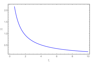
Figure 1: Profile of Hubble parameter $(H)$ against time (in billion years) for $k_{1}=1.59$, $k_{2}=0.7$, $k_{3}=1$, $m=3.59$, $c_{1}=c_{2}=1$.

Figure 2: Profile of Scale factor $(a)$ against time (in billion years) for $k_{1}=1.59$, $k_{2}=0.7$, $k_{3}=1$, $m=3.59$, $c_{1}=c_{2}=1$.

Figure 3: Profile of Metric potentials $A$ against time (in billion years) for $k_{1}=1.59$, $k_{2}=0.7$, $k_{3}=1$, $m=3.59$, $c_{1}=c_{2}=1$.

Figure 4: Profile of Metric potentials $B$ against time (in billion years) for $k_{1}=1.59$, $k_{2}=0.7$, $k_{3}=1$, $m=3.59$, $c_{1}=c_{2}=1$.

The profile of Hubble parameter, scale factor and metric potentials are presented in the Figures 1-4. Here we noticed from the Figure 1 that, Hubble parameter is a decreasing function of time and it approaches towards zero with the evolution of time. Scale factor and metric potentials are increasing function of time and they are approaching to infinity with the evolution of time i.e. $a,A,B\rightarrow\infty$ when $t\rightarrow\infty$.
The profile of energy density and pressure is presented in the Figure 6 and Figure 6 respectively. Here we noticed from the figure that, energy density is a decreasing function of time and it approaches towards zero with the evolution of time. Here the positivity of energy density, tighten the interval of $k_{2}$ from $0<k_{2}<2$ to $0.6<k_{2}<2$. The pressure of the model is also approaching to zero with the evolution of time and it is negative, which follow the observational data.
Figure 8 and Figure 8 represents the profile of cosmological constant and EoS parameter against time. The cosmological constant is positive and decreasing function of time. Here $\Lambda\rightarrow 0$ when $t\rightarrow\infty$. The EoS parameter is negative valued function and which is less than $-1$. It means that, our models represents the phantom energy cosmological model.

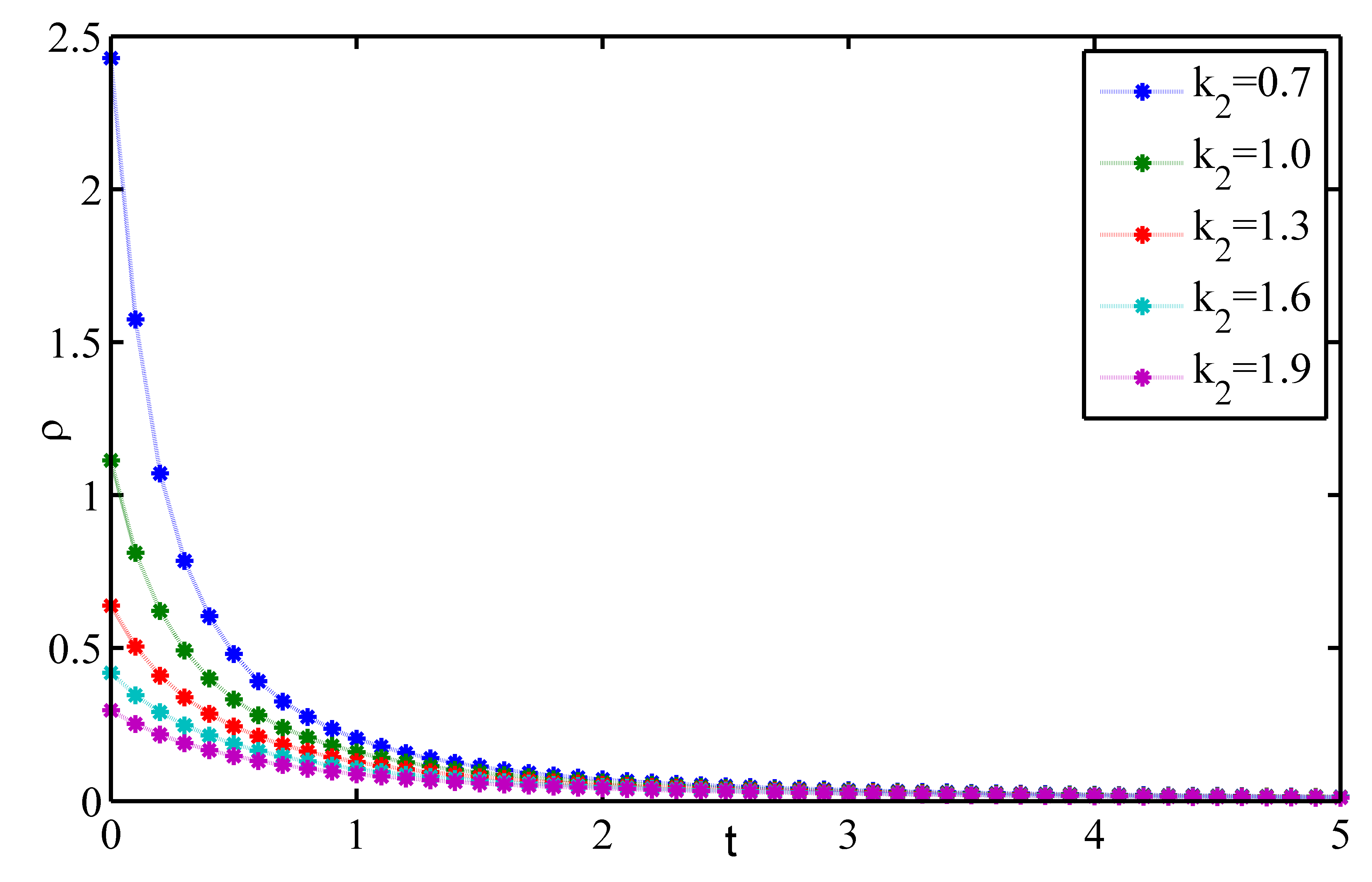
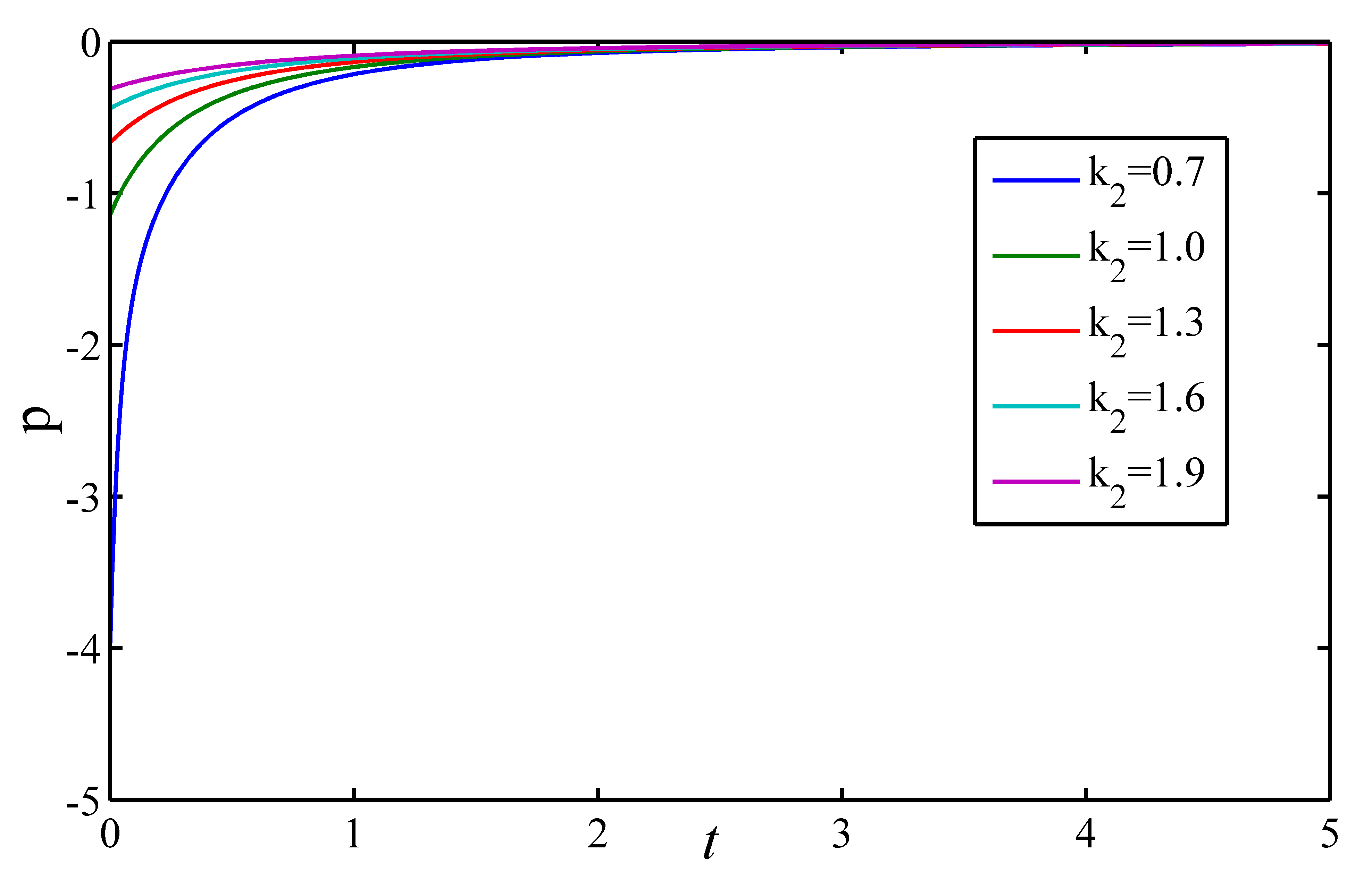
Figure 5: Profile for energy density against time for $k_{1}=1.59$, $k_{3}=1$, $m=3.59$, $c_{1}=c_{2}=1$ for various values of $k_{2}$.

Figure 6: Profile for pressure against time for $k_{1}=1.59$, $k_{3}=1$, $m=3.59$, $c_{1}=c_{2}=1$ for various values of $k_{2}$.

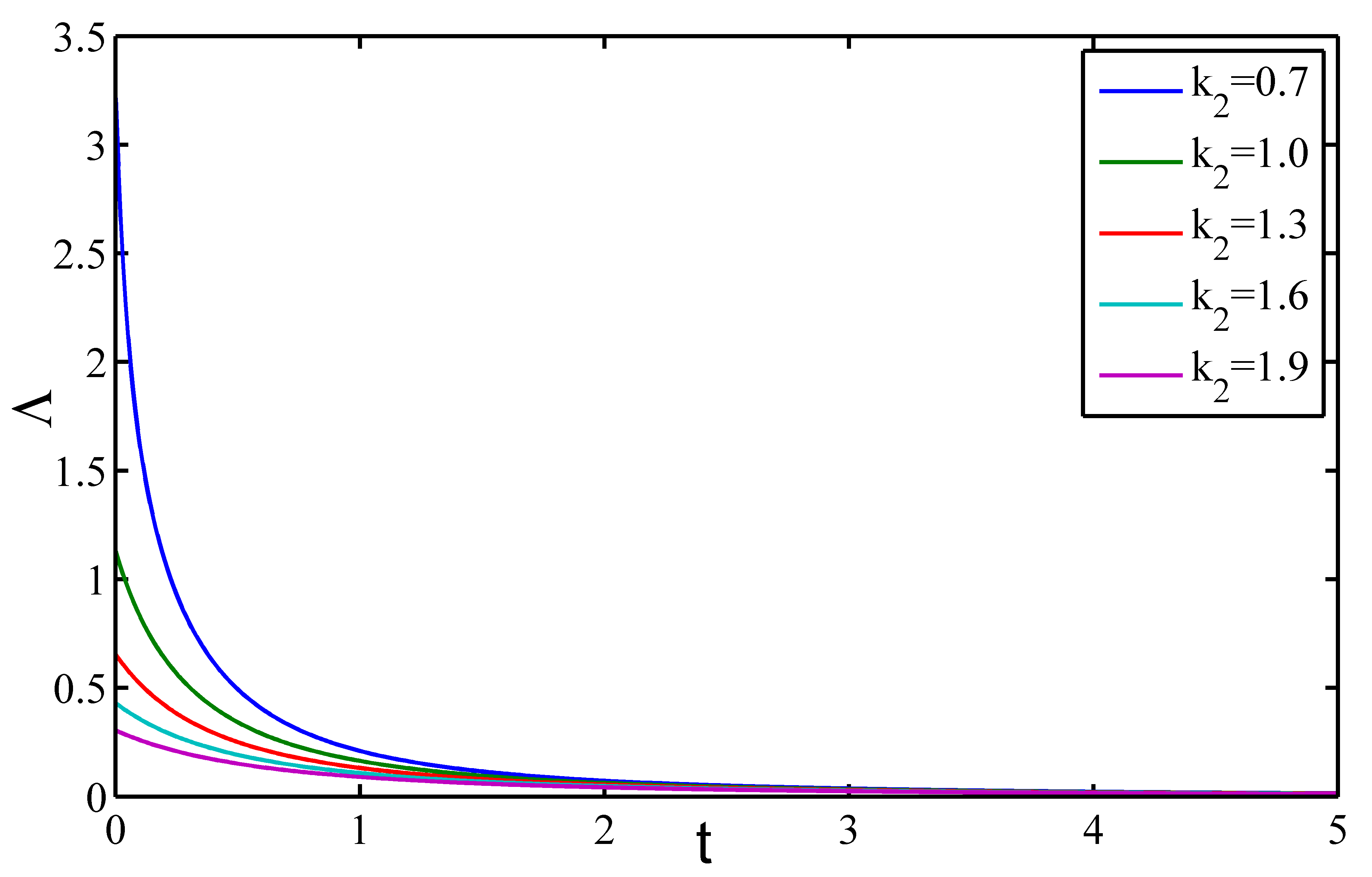
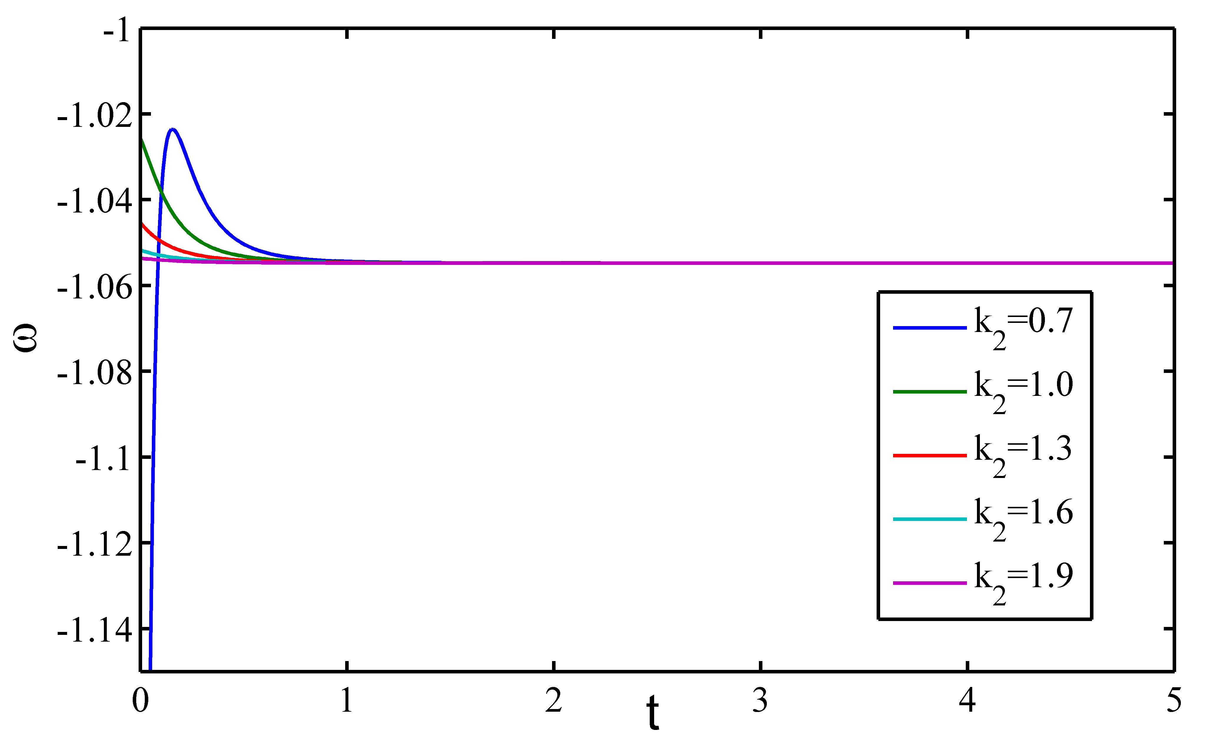
Figure 7: Profile for cosmological constant against time for $k_{1}=1.59$, $k_{3}=1$, $m=3.59$, $c_{1}=c_{2}=1$ for various values of $k_{2}$.

Figure 8: Profile for EoS parameter against time for $k_{1}=1.59$, $k_{3}=1$, $m=3.59$, $c_{1}=c_{2}=1$ for various values of $k_{2}$.

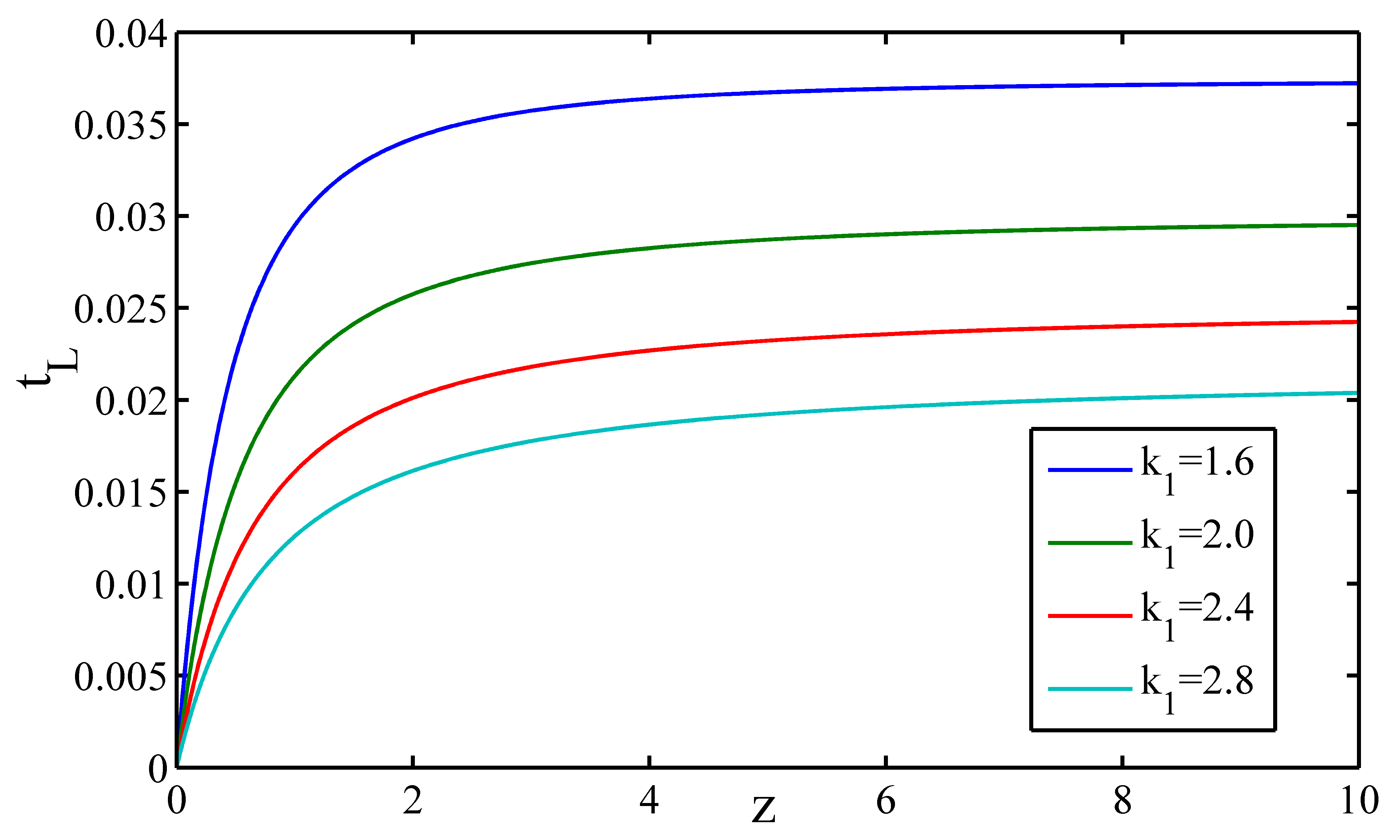
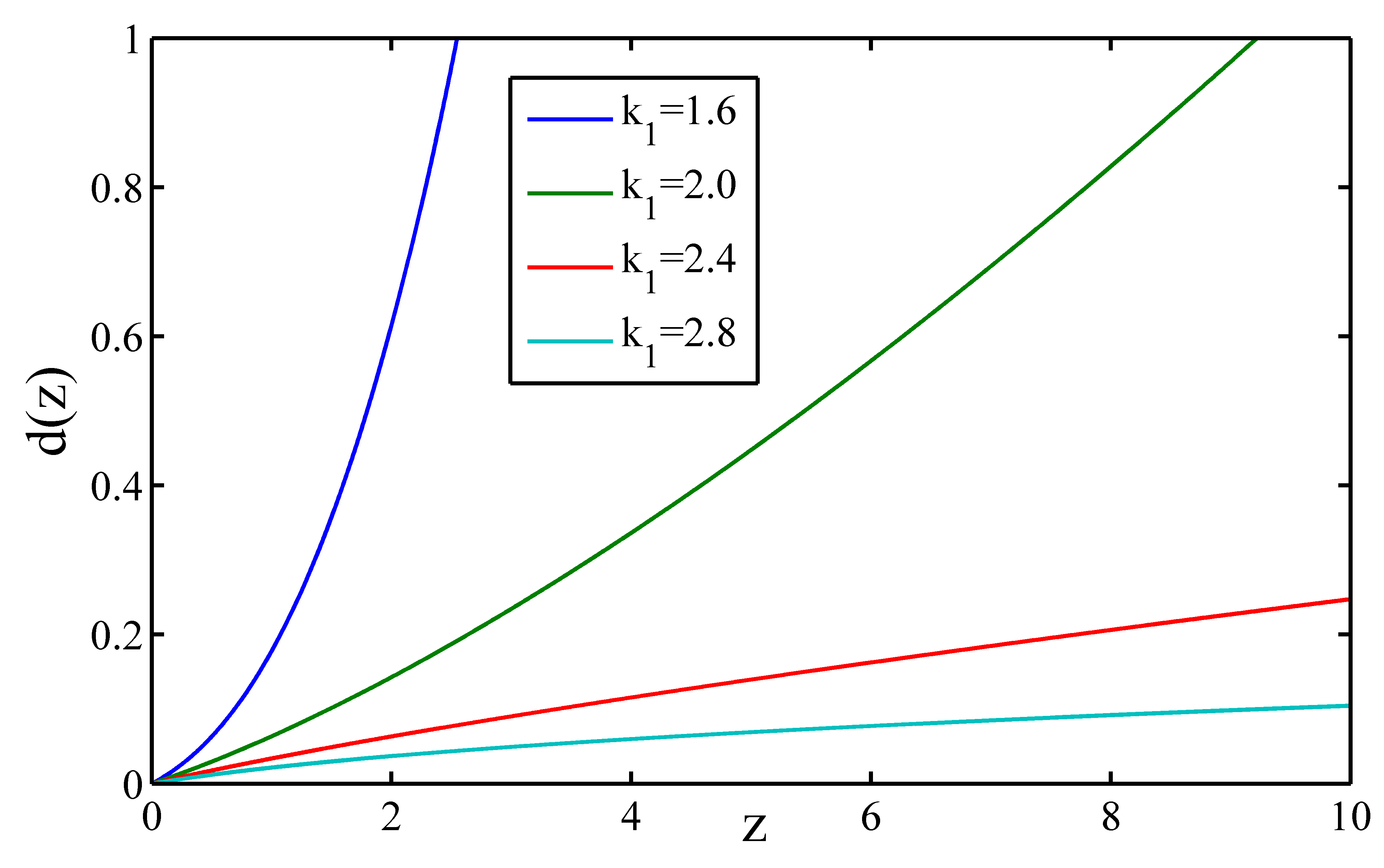
Figure 9: Profile for Look-back time against red-shift for $m=3.59$, $H_{0}=60$ for various values of $k_{1}$.

Figure 10: Profile for Proper distance against red-shift for $m=3.59$, $H_{0}=60$, $k_{3}=1$ for various values of $k_{1}$.

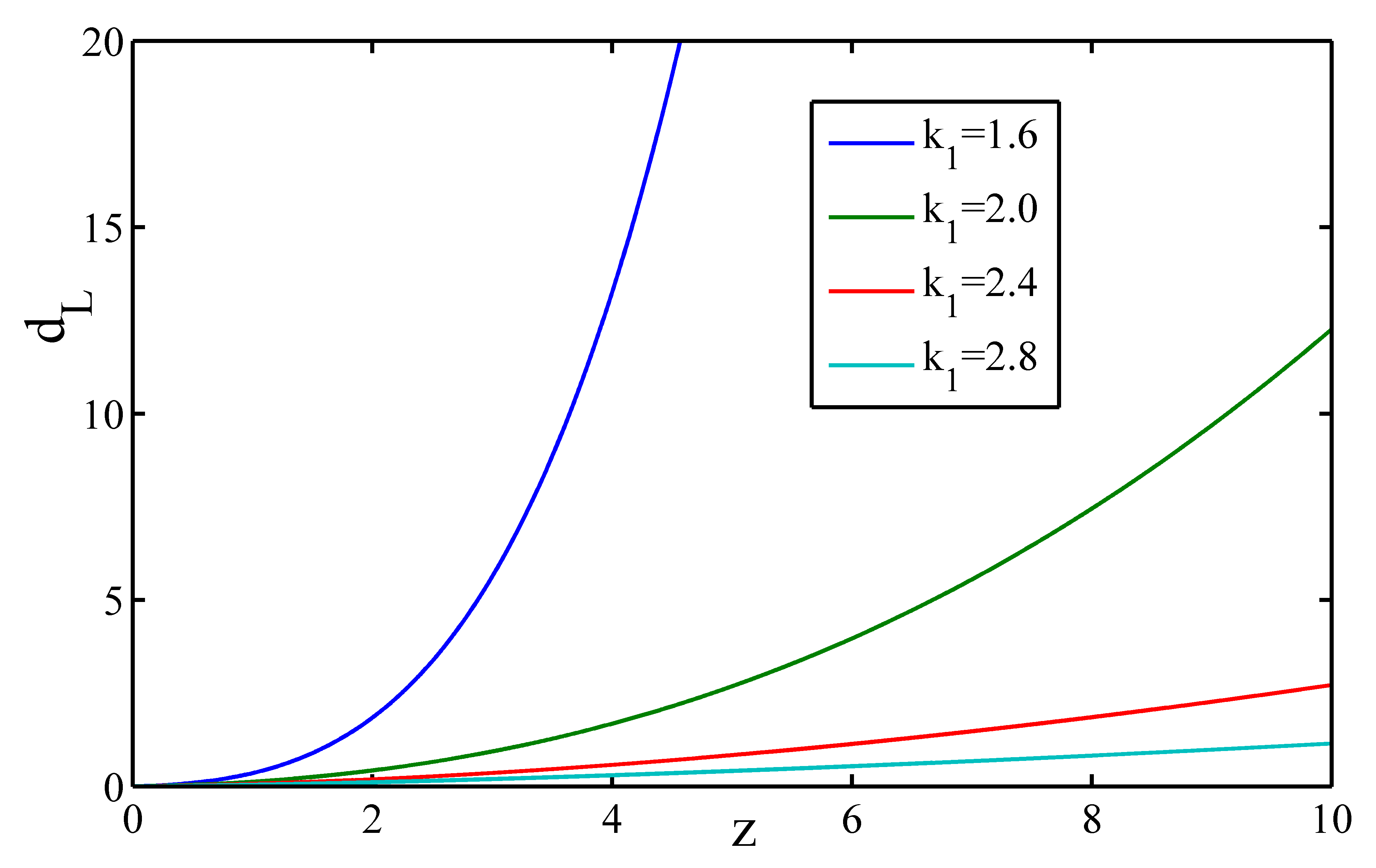
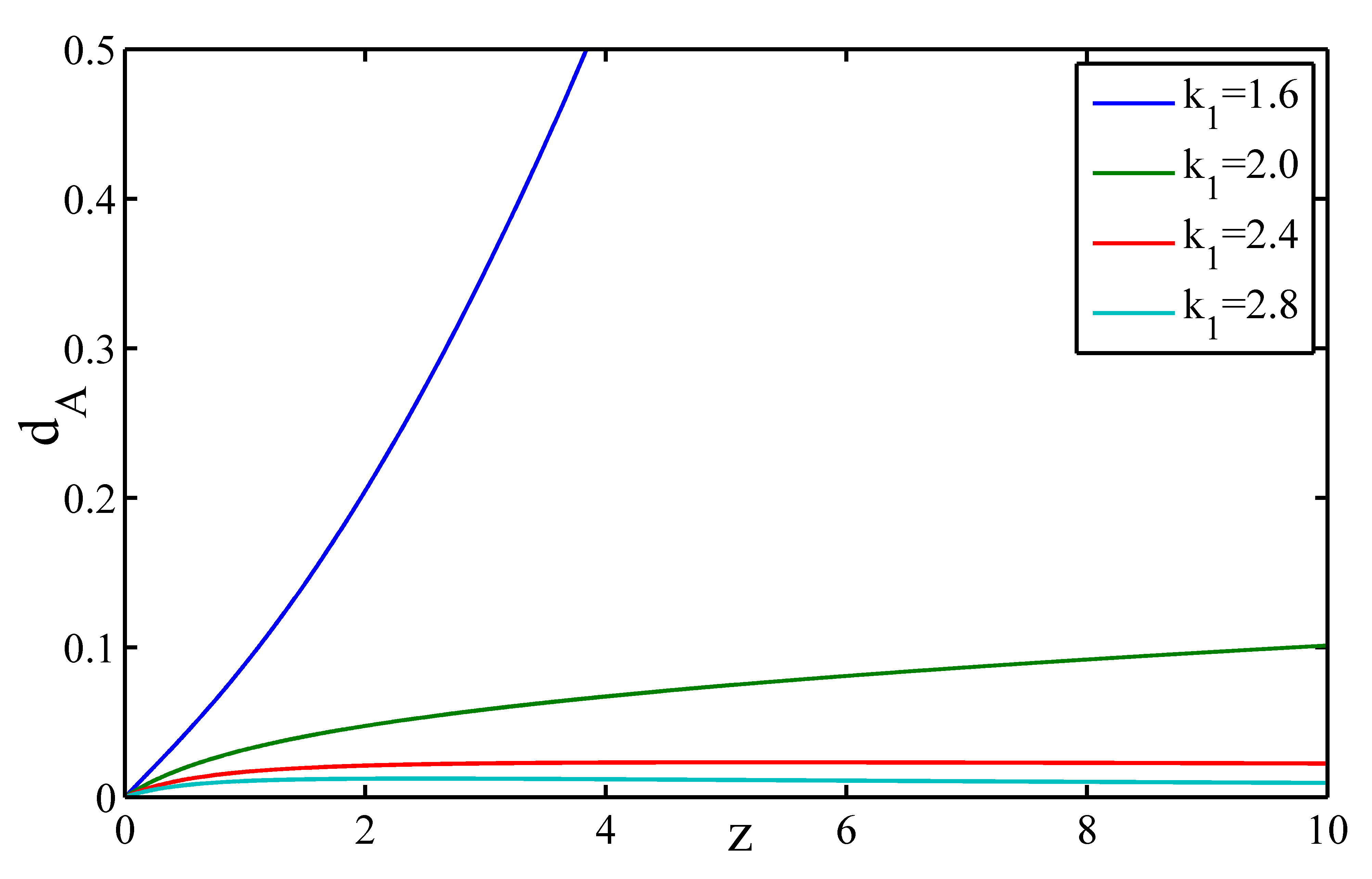
Figure 11: Profile for Luminosity distance against red-shift for $m=3.59$, $H_{0}=60$, $k_{3}=1$ for various values of $k_{1}$.

Figure 12: Profile for Angular-diameter distance against red-shift for $m=3.59$, $H_{0}=60$, $k_{3}=1$ for various values of $k_{1}$.

5 Distances in Cosmology

Distance is one of the basic measurement that we can performed. In the history of astronomy, distance measurement played a important role and some time surprising role for understanding about Universe. In this section, we have presented some of the different distance measures.

5.1 Look-back time-redshift

The look-back time $t_{L}$ is defined as the difference between the present age of the Universe $t_{0}$ and the age of the Universe, when a particular light from a cosmic source at a particular redshift $z$ was emitted. Thus it is defined as

$$t_{L}=t_{0}-t(z)=\int_{a}^{a_{0}}\frac{da}{\dot{a}},$$ (45)

where $a_{0}$ is the present day scale factor of the Universe. The scale factor of the Universe $a(t)$ is related to $a_{0}$ by the relation

$$\frac{a}{a_{0}}=\frac{1}{1+z}$$ (46)

For the discussed model, we have

$$k_{1}t+k_{2}=(k_{1}t_{0}+k_{2})(1+z)^{-\frac{m}{k_{1}}}$$ (47)

The above equation takes the form

$$H_{0}(t_{0}-t)=\frac{m}{k_{1}}\left[1-(1+z)^{-\frac{m}{k_{1}}}\right]$$ (48)

Here $H_{0}$ is the Hubble constant at present. The value of $H_{0}$ is lies between $50-100$ km s^-1 Mpc^-1. The equation (48) can also be expressed as

$$H_{0}(t_{0}-t)=\left(\frac{m}{k_{1}}\right)^{2}\left[z-\frac{m+k_{1}}{2k_{1}}z^{2}+\frac{(m+k)(m+2k)}{6k^{2}}z^{3}-\cdot\cdot\cdot\cdot\cdot\right]$$ (49)

With the help of $q=-1+\frac{k_{1}}{m}$, equation (49) takes the form

$$H_{0}(t_{0}-t)=\frac{1}{(1+q)^{2}}\left[z-\frac{2+q}{2(1+q)}z^{2}+\frac{(2+q)(3+2q)}{6(1+q)}z^{3}-\cdot\cdot\cdot\cdot\cdot\right]$$ (50)

When $z\rightarrow\infty$, equation (48) reads

$$t_{L}=t_{0}-t=\frac{m}{k_{1}}H_{0}^{-1}=\frac{H_{0}^{-1}}{1+q}$$ (51)

For small $z$, $H_{0}(t_{0}-t)$ can be approximated as

$$H_{0}(t_{0}-t)\approx\left(\frac{m}{k_{1}}\right)^{2}z=\frac{z}{(1+q)^{2}}$$ (52)

5.2 Proper Distance

The proper distance $d(z)$ is defined as the distance between a cosmic source emitting light at any instant $t=t_{1}$, located at $r=r_{1}$ with redshift $z$ and the observer receiving the light from the source emitted at $r=0$ and $t=t_{0}.$ Thus

$$d(z)=r_{1}a_{0},\;\text{where}r_{1}=\int_{t_{1}}^{t_{0}}\frac{dt}{a}$$ (53)

For the discussed model, we have the proper distance as

$$d(z)=\frac{mH_{0}^{-1}}{k_{3}(k_{1}-m)}\left[1-(1+z)^{-\frac{m}{k_{1}}(1-\frac{m}{k_{1}})}\right]$$ (54)

The above expression indicates that, $d(z)\rightarrow\frac{mH_{0}^{-1}}{k_{3}(k_{1}-m)}$ when $z\rightarrow\infty$ for $0<\frac{m}{k_{1}}<1$ and $d(z)\rightarrow\infty$ when $z\rightarrow\infty$ for $\frac{m}{k_{1}}\geq 1$.

5.3 Luminosity distance

The apparent luminosity of a source at radial coordinate $r_{1}$ with a redshift $z$ of any size $l$ is defined as

$$l=\frac{L}{4\pi r_{1}^{2}a_{0}^{2}(1+z)^{2}},$$ (55)

where $L$ is the absolute luminosity distance. Let us introduce a luminosity distance $d_{L}$ as

$$d_{L}=\left(\frac{L}{4\pi l}\right)=a_{0}r_{1}(1+z)$$ (56)

With the help of equation (53), equation (56) takes the form

$$d_{L}=d(z)(1+z)$$ (57)

For the discussed model, we have Luminosity distance $d_{L}$ as

$$d_{L}=\frac{mH_{0}^{-1}}{k_{3}(k_{1}-m)}\left[1-(1+z)^{-\frac{m}{k_{1}}(1-\frac{m}{k_{1}})}\right](1+z)$$ (58)

5.4 Angular-diameter distance

The angular-diameter distance $d_{A}$ is defined such that

$$\theta=\frac{l}{d_{A}},$$

where $\theta$ is the angle subtended by an object of size $l$. It is also defined in term of proper distance and Luminosity distance as

$$d_{A}=d(z)(1+z)^{-1}=d_{L}(1+z)^{-2}.$$

For the presented model

$$H_{0}d_{A}=\frac{m}{k_{3}(k_{1}-m)}\left[1-(1+z)^{-\frac{m}{k_{1}}(1-\frac{m}{k_{1}})}\right](1+z)^{-1}.$$ (59)

5.5 Distance Modulus

The distance modulus $(\mu(z))$ is given as

$$\mu(z)=5\log d_{L}+25$$

Thus, the distance modulus $(\mu(z))$ in terms of redshift parameter $z$ is obtained as

$$\mu(z)=5\log\left(\frac{mH_{0}^{-1}}{k_{3}(k_{1}-m)}\left[1-(1+z)^{-\frac{m}{k_{1}}(1-\frac{m}{k_{1}})}\right]\right)+25$$ (60)

6 Conclusion

In this article, we have presented a new solution to the field equations by using the law of variation for Hubble’s parameter which yield constant deceleration parameter. The law of variation for Hubble parameter in Eq. (31) explicitly determine the values of the scale factors. One can solve Einstein field equations for Bianchi type metric with this functional form of Hubble parameter in principle. For $k_{1}=0$, the deceleration parameter $q=-1$ and $\frac{dH}{dt}=0$, which gives the greatest value of $H$ and fastest rate of expansion as presented in Figure 1. This type of solutions are consistent as per the recent observations for an accelerated expansion of the universe. The variation of Hubble parameter presented in this paper may be used to study new solutions of Einstein field equations in modified theories of gravity. The model obtained in Eq. (44) of the universe start with a singularity at $t=-\frac{k_{2}}{k_{1}}$ and remain regular in finite region. The expansion rate goes down with time and finally tend to zero as $t\rightarrow\infty$. From the anisotropy parameter, it is observed that the model of the universe remains anisotropic throughout the evolution. The energy density approaches to zero as $t\rightarrow\infty$. The EoS parameter clearly shows that this model is in phantom region. Finally, we have discussed the consistency of this model with the distance parameters such as look back time, proper distance, luminosity distance, angular diameter distance and the distance modulus (see Figure 10 to Figure 12).

7 Acknowledgements

Author SKJP wish to thank National Board of Higher Mathematics, Department of Atomic Energy (DAE), Government of India for financial support through post doctoral research fellowship. Author PKS wish to thank M. Sami for his support and CTP, JMI for hospitality where a part of this work have been done. We are very indebted to the editor and the anonymous referee for illuminating suggestions that have significantly improved our paper in terms of research quality as well as presentation.

References

- [1] S. Capozziello et al. , Phys. Rev. D 71 (2005) 043503.
- [2] S. Nojiri, S. D. Odintsov, Phys. Rev. D 74 (2006) 086005.
- [3] S. Nojiri, S. D. Odintsov, Int. J. Geom. Meth. Mod. Phys 4 (2006) 115. arXiv:hep-th/0601213
- [4] S. Nojiri, S. D. Odintsov, Phys. Rev. D 77 (2008) 026007.
- [5] S. Nojiri, S. D. Odintsov, Phys. Rept. 505 (2011) 59. arXiv:1011.0544
- [6] S. Capozziello, M. De Laurentis , Phys. Rept. 509 (2011) 167. arXiv:1108.6266
- [7] S. Nojiri, S. D. Odintsov, V. K. Oikonomou, arXiv:1705.11098
- [8] W. Hu, I. Sawicki, Phys. Rev. D 76 (2007) 064004.
- [9] S. A. Appleby, R. A. Battye, Phys. Lett. B 654 (2007) 7.
- [10] A. A. Starobinsky, JETP Lett. 86 (2007) 156.
- [11] S. Nojiri, S. D. Odintsov, Int. J. Geom. Methods Mod. Phys. 4 (2007) 115.
- [12] S. Nojiri, S. D. Odintsov, Mod. Phys. Lett. A 29 (2014) 1450211. arXiv:1408.3561
- [13] S. D. Odintsov, V. K. Oikonomou, Annals of Physics, 363 (2015) 503. arXiv:1508.07488
- [14] S. D. Odintsov, V. K. Oikonomou, Astrophys. Space Sci., 361 (2016) 174. arXiv:1512.09275
- [15] T. Harko, F. S. N. Lobo, S. Nojiri, S. D. Odintsov, Phys. Rev. D 84 (2011) 024020.
- [16] A. Salehi, S. Aftabi , J. High Energ. Phys. 2016 (2016) 140.
- [17] M. J. S. Houndjo, Int. J. Mod. Phys. D 21 (2012) 1250003.
- [18] M. Sharif, M. Zubair, JCAP 03 (2012) 028.
- [19] M. Sharif, S. Rani, R. Myrzakulov, Eur. Phys. J. Plus 128 (2013) 123.
- [20] A. F. Santos, Mod. Phys. Lett. A, 28 (2013) 1350141.
- [21] A. F. Santos, C. J. Ferst, Mod. Phys. Lett. A 30 (2015) 1550214.
- [22] D. Momeni, P. H. R. S. Moraes, R. Myrzakulov, Astrophys. Space Sci. 361 (2016) 228.
- [23] C. P. Singh, P. Kumar, Eur. Phys. J. C 74 (2014) 3070.
- [24] Shri Ram, S. Chandel, Astrophys Space Sci. 355 (2015) 195.
- [25] M. F. Shamir, Z. Raza, Astrophys Space Sci. 356 (2015) 111.
- [26] P. H. R. S. Moraes, J. D. ArbaÃil, M. Malheiro, JCAP 06 (2016) 005.
- [27] A. Alhamzawi, R. Alhamzawi, Int. J. Mod. Phys. D 25 (2016) 1650020.
- [28] P. H. R. S. Moraes, Int. J. Theor. Phys. 55 (2016) 1307.
- [29] M. E. S. Alves, P. H. R. S. Moraes, J. C. N. de Araujo, M. Malheiro, Phys. Rev. D 94 (2016) 024032.
- [30] Z. Yousaf, Kazuharu Bamba, M. Zaeem-ul-Haq Bhatti, Phys. Rev. D 93 (2016) 124048.
- [31] M. Zubair, I. Noureen, Eur. Phys. J. C 75 (2015) 265.
- [32] I. Noureen, M. Zubair, Eur. Phys. J. C 75 (2015) 62.
- [33] D. R. K. Reddy, R. Santi Kumar: Astrophys. Space Sci. 344 (2013) 253.
- [34] P. K. Sahoo, M. Sivakumar, Astrophys Space Sci 357 (2015) 60.
- [35] G. P. Singh, B. K. Bishi, Astrophys. Space Sci. 360 (2015) 34.
- [36] D. Sofuoglu, Astrophys. Space Sci., 361 (2016) 12.
- [37] P. K. Sahoo, Parbati Sahoo, B. K. Bishi, Int. J. Geom. Methods Mod. Phys. 14 (2017) 1750097.
- [38] P. K. Sahoo, Parbati Sahoo, B. K. Bishi, S. Aygun, Mod. Phys. Lett. A 32 (2017) 1750105.
- [39] S. K. J. Pacif, R. Myrzakulov, S. Myrzakul, Int. J. Geom. Methods Mod. Phys., 15 (2017) 1750111.
- [40] S. K. J. Pacif, B. Mishra, Res. Astron. Astrophys. 15 (2015) 2141.