Consistent Scalar and Tensor Perturbation Power Spectra in Single Fluid Matter Bounce with Dark Energy Era

Abstract

We investigate cosmological scenarios containing one canonical scalar field with an exponential potential in the context of bouncing models, where the bounce happens due to quantum cosmological effects. The only possible bouncing solutions in this scenario (discarding an infinitely fine tuned exception) must have one and only one dark energy phase, either occurring in the contracting era or in the expanding era. Hence, these bounce solutions are necessarily asymmetric. Naturally, the more convenient solution is the one where the dark energy phase happens in the expanding era, in order to be a possible explanation for the current accelerated expansion indicated by cosmological observations. In this case, one has the picture of a Universe undergoing a classical dust contraction from very large scales, the initial repeller of the model, moving to a classical stiff matter contraction near the singularity, which is avoided due to the quantum bounce. The Universe is then launched to a dark energy era, after passing through radiation and dust dominated phases, finally returning to the dust expanding phase, the final attractor of the model. We calculate the spectral indexes and amplitudes of scalar and tensor perturbations numerically, considering the whole history of the model, including the bounce phase itself, without making any approximation or using any matching condition on the perturbations. As the background model is necessarily dust dominated in the far past, the usual adiabatic vacuum initial conditions can be easily imposed in this era. Hence, this is a cosmological model where the presence of dark energy behavior in the Universe does not turn problematic the usual vacuum initial conditions prescription for cosmological perturbation in bouncing models. Scalar and tensor perturbations end up being almost scale invariant, as expected. The background parameters can be adjusted, without fine tunings, to yield the observed amplitude for scalar perturbations, and also for the ratio between tensor and scalar amplitudes, $r=T/S\lesssim 0.1$. The amplification of scalar perturbations over tensor perturbations takes place only around the bounce, due to quantum effects, and it would not occur if General Relativity has remained valid throughout this phase. Hence, this is a bouncing model where a single field induces not only an expanding background dark energy phase, but also produces all observed features of cosmological perturbations of quantum mechanical origin at linear order.

I Introduction

Bouncing models have been proposed as cosmological scenarios without an initial singularity. Instead, the Universe had at least a preceding contracting phase from very large length scales, shrinking the space until the scale factor reaches a minimum value in which some new physics takes place, mainly related to gravity modifications at very small length scales, halting the contraction and launching the Universe into the expanding phase we are living in.

In the standard cosmological model, inflation is responsible for exponentially increase the particle horizon after the Big Bang in order to explain why regions, which are not in causal contact at the last scattering surface, present a highly correlated temperature distribution, as observed today in the Cosmic Microwave Background radiation (CMB). Without inflation, these regions would be causally disconnected in a purely Big Bang model. This puzzle is the so called horizon problem, and it does not exist in bouncing models. Since the Universe had a very large period of contraction in the past, there is no limit to the particle horizon (if the fluids dominating the contracting phase satisfy the strong energy condition). Another puzzle of a purely Big Bang scenario is the flatness problem, i.e., considering a Friedmann metric in a expanding phase, the spatial curvature dilutes slower than any other matter content (assuming again the strong energy condition) of the model. Hence, unless the spatial curvature is strongly fine tuned to zero initially, it would quickly dominates the expansion afterwards. When inflation is added to the Big Bang scenario, it turns out that the Universe is driven dynamically to an almost flat hypersurface, avoiding the initial curvature fine tuning problem. In the bounce scenario this issue is not posed, since flat space-like hypersurfaces are dynamical attractors during contraction Peter and Pinto-Neto (2008); Brandenberger (2012).

Despite the fact that inflation has not yet any consensual fundamental physics behind it, a simple slow-roll prescription for the inflation scalar field is enough to solve the above mentioned puzzles, and to amplify quantum vacuum fluctuations after the Big Bang, thus giving rise to an almost scale invariant adiabatic power spectrum, in good agreement with CMB observations Planck Collaboration et al. (2015a). It is a challenge for bounce cosmologies to reproduce a competitive fit for the observations, and many models have been scrutinized over the years with this aim.

In what concerns the primordial phase of bounce cosmologies, it has been shown that perturbations originated from quantum vacuum fluctuations during a matter dominated contraction phase become almost scale invariant Wands (1999); Finelli and Brandenberger (2002); Pinho and Pinto-Neto (2007) in the expanding phase. Whether the linear perturbation theory remains valid for a specific gauge choice through the bounce is a subtle question addressed by many authors Cartier et al. (2003); Martin and Peter (2003, 2004); Allen and Wands (2004), and finally clarified in Refs.Vitenti and Pinto-Neto (2012); Pinto-Neto and Vitenti (2014), confirming the validity of linear perturbation theory up to the expanding phase. The background scenarios used to developed those investigations are matter contractions driven either by a canonical scalar field with an exponential potential, a K-essence scalar field representing a hydrodynamical fluid, or a relativistic perfect fluid using Schutz formalism Schutz (1970, 1971). This scenario with a contracting phase dominated by a dust-like fluid is called matter bounce scenario. This class of models is an interesting new approach to the Big Bang/Inflation scenario Brandenberger (2012); Allen and Wands (2004); Peter and Pinto-Neto (2008); Cai et al. (2012), and they have been extensively studied over the past 15 years. A weak point for any model including a contracting phase, where all the matter content satisfy the dominant energy condition, is the presence of Belinsky-Khalatnikov-Lifshitz (BKL) instabilities Belinskii et al. (1970); Battefeld and Peter (2015); Karouby et al. (2011); Brandenberger and Peter (2016), the fast growth of anisotropies during the contraction. Some proposals inspired in the Ekpyrotic Model Khoury et al. (2001) address this problem by means of an ad-hoc ekpyrotic type potential Cai et al. (2013). It is not the aim of this work to address this kind of issue, since it is possible to overcome it in more complex scenarios without completely spoiling out a suitable primordial power spectra. Note that any cosmological model, either inflationary, bouncing, or any other, has a much more serious problem to deal with: the large degree of initial homogeneity necessary to turn all these models compatible with observations. This is largely more serious than the BKL problem. Note also that once one assumes an initial homogeneous and isotropic Universe, one can show for the models we are considering that the shear perturbation will never overcome the background degrees of freedom, even growing as fast as $a^{-6}$ in the contracting phase Pinto-Neto and Vitenti (2014), and hence the BKL problem is not present once such assumption is made. For a discussion on that, see also Ref. Celani et al. (2017).

In this paper we will carefully study the physical properties of primordial quantum perturbations in a matter bounce realized by a canonical scalar field with an exponential potential. Our starting point are the results obtained in Refs. Heard and Wands (2002); Colistete et al. (2000). In our scheme, we will argue that, approaching the singularity during contraction, quantum effects as calculated in Ref. Colistete et al. (2000) become relevant, and a bounce arises naturally in the context of the canonical quantization of gravity, connecting the classical contracting and expanding phases described in Ref. Heard and Wands (2002). The known cosmological solutions obtained through the de Broglie-Bohm (dBB) formulation of quantum mechanics can be applied to this system since the classical singularity takes place when the kinetic term dominates the scalar field dynamics, and the potential becomes negligible, exactly as in the model investigated in Ref. Colistete et al. (2000). Hence, one has classical contracting and expanding phases connected by a quantum bounce. Our background model avoids the need of a ghost scalar field and is sustained by the fact that, in the regime where the curvature scale is $10^{2}$ Planck length or larger, the canonical quantization we implement is expected to be an effective limit of more fundamental theories of quantum gravity. Finally, since the perturbations evolve through the background quantum phase, we use the right action for the perturbations when the background is not assumed to be classical Falciano et al. (2013).

Our dynamical system analysis shows that this scenario carries an interesting feature: as we will see, if a bounce takes place in between classical contracting and expanding phases, the scalar field presents an effective transient dark energy-type Equation of State (EoS), either in the past of the contracting phase or in the future of the expanding phase. This addresses an aspect of bouncing cosmologies that has gained increased attention Zhang et al. (2007); Lehners and Steinhardt (2009); Jamil et al. (2011); Maier et al. (2011); Brevik et al. (2014); Odintsov and Oikonomou (2016): the role of the dark energy (DE) in the contracting phase of bouncing models. In the expansion history probed by current observations, the effects due to the existence of a DE component can only be felt when the scale factor is of about 3-4 e-folds from the last scattering surface Dodelson (2003). Whether the DE is a cosmological constant or a quintessence field, it should be present during the contracting phase too. Thus, it may affect the contracting phase evolution of perturbations sensible to scales around the same Hubble radius as today. The presence of dark energy in the contracting phase of bouncing models may turn problematic the imposition of vacuum initial conditions for cosmological perturbations in the far past of such models. For instance, if dark energy is a simple cosmological constant, all modes will eventually become larger than the curvature scale in the far past, and an adiabatic vacuum prescription becomes quite contrived, see Ref. Maier et al. (2011) for a discussion on this point. However, in the case of a scalar field with exponential potential, which contains a transient dark energy phase, the Universe will always be dust dominated in the far past, and adiabatic vacuum initial conditions can be easily imposed in this era, as usual. Hence, this is a situation where the presence of dark energy does not turn problematic the usual initial conditions prescription for cosmological perturbations in bouncing models.

The bounce solutions obtained here are necessarily asymmetric, i.e., the transient DE is effective either in the contracting phase or in the expanding phase, but not in both. Here we will study the more realistic solution where the dark energy phase happens in the expanding era, connecting the bounce model with the current accelerated expansion phase. Hence one has the picture of a Universe which realizes a dust contraction from very large scales, the initial repeller of the model, moves to a stiff matter contraction near the singularity and realizes a quantum bounce that ejects the Universe in a stiff matter expanding phase. The latter moves to a dark energy era, finally returning to the dust expanding phase, the final attractor of the model. The other possibility, DE in the contracting phase, is more academic, and we let it for a future work. The background solutions are constructed numerically, matching the classical and quantum eras in the phase where both have the similar dynamics.

Note that it can already be found in the literature exact solutions of the full Wheeler-DeWitt equation for a canonical scalar field with exponential potential, which is not neglected in the quantum phase Colin and Pinto-Neto (2017). These solutions were obtained without matchings. However, as they have exactly the same physical features as the solutions described above (classical behavior up to stiff matter domination, where quantum effects begin to be important and the potential is negligible, and one and only one DE energy phase all along), we preferred to adopt the above matching procedure, in which the numerical calculations are simpler to handle.

After the background construction, scalar and tensor perturbations are calculated numerically, and the results are understood analytically. Depending on the parameters of the background, they turn out to be almost scale invariant, with the right observed amplitude for scalar perturbations, and also for the ratio between tensor and scalar amplitudes, $r=T/S\lesssim 0.1$. The amplification of scalar perturbations over tensor perturbations takes place only around the bounce, and we explicitly show that it happens due to the quantum effects on the background model producing the bounce. There are many papers pointing out the difficulties of producing this amplification of scalar perturbations over tensor perturbations in the framework of General Relativity (GR), see Refs. Allen and Wands (2004); Xue et al. (2013); Battarra et al. (2014). Indeed, the amplification we will present would not occur if GR has remained valid all along the bounce. Hence, our result shows that when GR is violated around the bounce, the influence of this phase on the evolution of cosmological perturbations can be nontrivial, and must be evaluated with care. These effects provide a counter example to the usual case where the perturbations are unaffected by the details of the bounce and their amplitude are determined by the bounce depth (the ratio between the value of the scale factor during the potential crossing and its value at the bounce).

The paper will be divided as follows: in Sec. II, based on Ref. Heard and Wands (2002), we summarize the classical minisuperspace model and its full space of solutions. In Sec. III, we present the quantum background near the singularity, as presented in Ref. Colistete et al. (2000). The matching of the classical and quantum solutions is explained in Sec. IV, where we obtain the full background model with reasonable observational properties. Section VI describes the equations of motion for the quantum perturbations with suitable vacuum initial conditions, and we perform the numerical calculations in Sec. VII, exhibiting our final results for both scalar and tensor perturbations. We conclude in Sec. VIII with discussions and perspectives for future work.

In what follows we will consider $\hbar=c=1$ and the reduced Planck mass $M_{{}_{\mathrm{P}}}\equiv 1/\kappa\equiv 1/\sqrt{8\pi G_{{}_{\mathrm{N}}}}$. The metric signature is $(+,-,-,-)$.

II Background

We consider a canonical scalar field $\phi$ whose Lagrangian density is given by

$$\mathcal{L}=\sqrt{-g}\left[\nabla^{\nu}\phi\nabla_{\nu}\phi-V(\phi)\right].$$ (1)

The potential $V(\phi)$ is chosen to be the exponential, i.e.,

$$V(\phi)=V_{0}\mathrm{e}^{-\lambda\kappa\phi},$$ (2)

where the constant $V_{0}$ has units $\mathrm{mass}^{4}$ and $\lambda$ is dimensionless.

The exponential potential has vastly assisted cosmologists to address puzzles of the standard model because of its rich dynamics. In Refs. Chang and Scherrer (2016); Chen et al. (2016); Danila et al. (2016); Forte (2016); Granda and Loaiza (2016); Harko et al. (2017); Oikonomou (2016) we have some heterogeneous collection of what was published with exponential potential only in 2016. For the background dynamics, we will use results from Halliwell (1987); Copeland et al. (1998); Kolda and Lahneman (2001); Heard and Wands (2002); Allen and Wands (2004).

In a flat, homogeneous and isotropic Universe, the Friedmann-Lamâitre-Robertson-Walker metric is

$$\mathrm{d}s^{2}=N^{2}(\tau)\mathrm{d}\tau^{2}-a(\tau)^{2}(\mathrm{d}x^{2}+\mathrm{d}y^{2}+\mathrm{d}z^{2}),$$ (3)

where $N(\tau)$ is the lapse function and $a(\tau)$ is the scale factor. The evolution of the scale factor in cosmic time ($N(\tau)=1,\;\tau=t$) is given by the Friedmann equation coupled to the Klein-Gordon equation, respectively,

$$\dot{a} =aH,$$ (4)

$$\dot{H} =-\frac{\kappa^{2}}{2}\dot{\phi}^{2},$$ (5)

$$\ddot{\phi} =-3H\dot{\phi}-\frac{\mathrm{d}V}{\mathrm{d}\phi},$$ (6)

where the dot operator represents the derivative with respect to the cosmic time $t$. The Hubble function, $H$, must satisfy the Friedmann constraint

$$H^{2}=\frac{\kappa^{2}}{3}\left[\frac{\dot{\phi}^{2}}{2}+V(\phi)\right].$$ (7)

The background dynamics can be made simpler through a choice of dimensionless variables that allows us to rewrite the coupled second order equations (5) and (6) as a planar system Wainwright and Ellis (2005), i.e.,

$$x=\frac{\kappa\dot{\phi}}{\sqrt{6}H},\qquad y=\frac{\kappa\sqrt{V}}{\sqrt{3}H}.$$ (8)

In those new variables, the Friedmann constraint, Eq. (7), and the effective EoS read,

$$x^{2}+y^{2}=1,\qquad w=2x^{2}-1.$$ (9)

Applying the above definitions to the system of Eqs. (5) and (6) leads to the planar system:

$$\frac{\mathrm{d}x}{\mathrm{d}\alpha} =-3x(1-x^{2})+\lambda\sqrt{\frac{3}{2}}y^{2},$$ (10)

$$\frac{\mathrm{d}y}{\mathrm{d}\alpha} =xy\left(3x-\lambda\sqrt{\frac{3}{2}}\right),$$ (11)

where $\alpha\equiv\ln(a)$. This system is supplemented by the equations

$$\dot{\alpha}=H,\qquad\dot{H}=-3H^{2}x^{2}.$$ (12)

The critical points are listed in Tab. 1.

$x$	$y$	$w$
$-1$	$0$	$1$
$1$	$0$	$1$
$\frac{\lambda}{\sqrt{6}}$	$-\sqrt{1-\frac{\lambda^{2}}{6}}$	$\frac{1}{3}\left(\lambda^{2}-3\right)$
$\frac{\lambda}{\sqrt{6}}$	$\sqrt{1-\frac{\lambda^{2}}{6}}$	$\frac{1}{3}\left(\lambda^{2}-3\right)$

Table 1: Critical points of the planar system Eqs. (10) and (11).

Near the critical points where $w=1$, the effective energy density of the scalar field evolves close to $a^{-6}$, i.e., it behaves approximately like a stiff-matter fluid. For those where the effective EoS is $w=\frac{1}{3}\left(\lambda^{2}-3\right)$, it evolves as $a^{-\lambda^{2}}$. The qualitative behavior of the system can be studied with the tools described in Wainwright and Ellis (2005); Coley (1999); Boehmer and Chan (2014), for a detailed analysis see Heard and Wands (2002); Copeland et al. (1998); Kolda and Lahneman (2001); Allen and Wands (2004).

In the contracting phase $H<0$, we can see by the definition of $y$, Eq. (8), that $y<0$. Note that $y$ is completely determined by the value of $x$ through the constraint (9) and the sign of $H$. This phase is, therefore, tied to the lower quadrants of the phase space, while the upper quadrants depict the expanding phase, see Fig. 1. Using the Friedmann constraint Eq. (10) yields

$$\frac{\mathrm{d}x}{\mathrm{d}\alpha}=-3\left(x-\frac{\lambda}{\sqrt{6}}\right)\left(1-x\right)\left(1+x\right).$$ (13)

For $\lambda<\sqrt{6}$, the first two critical points, $x_{\pm{}c}=\pm 1$ and $y_{\pm{}c}=0$, are unstable (repellers) during expansion and stable (attractors) in the contraction phase, i.e.,

$$\left.\frac{\mathrm{d}x}{\mathrm{d}\alpha}\right|_{x=1-\epsilon}<0,\qquad\left.\frac{\mathrm{d}x}{\mathrm{d}\alpha}\right|_{x=-1+\epsilon}>0,$$

for $0<\epsilon\ll 1$. For $\lambda>0$, the critical point $x_{\lambda}={\lambda}/{\sqrt{6}}$ has the following behavior,

$$\left.\frac{\mathrm{d}x}{\mathrm{d}\alpha}\right|_{x=\frac{\lambda}{\sqrt{6}}+\epsilon}<0,\qquad\left.\frac{\mathrm{d}x}{\mathrm{d}\alpha}\right|_{x=\frac{\lambda}{\sqrt{6}}-\epsilon}>0.$$

It is, therefore, an attractor during the expanding phase and an a repeller in a contracting phase.

For the purpose of this work, we will choose $\lambda=\sqrt{3}$. As a consequence, the scalar field behaves as a matter-fluid, $w=0$, around the critical point $x_{\lambda}$. Then, choosing the initial conditions for $x$, as

$$x_{\lambda}=\frac{\lambda}{\sqrt{6}}\pm\epsilon,$$ (14)

leads to a matter-fluid contracting phase. Since $x_{\lambda}$ is the only attractor in the expanding phase, the model will always end in matter-fluid dominated epoch.

In Fig. 1 we have the phase space for the planar system. The critical points in which the scalar field behaves as a stiff-matter fluid are marked as $\mathrm{S_{\pm}}$ and the ones it behaves as a matter-like fluid are $\mathrm{M_{\pm}}$. The contraction history goes as follows: the Universe starts close to the critical point $M_{-}$ and, depending on the choice of sign in Eq. (14), arrives at the stable point $S_{+}$ or $S_{-}$ for, respectively $+$ and $-$. The evolution then ends up in a singularity (if no quantum effects are included). The final EoS parameter is $w=1$. Classically, there is no possible bounce solution when the system arrives in the critical points $S_{\pm}$.

In the trajectories $M_{-}\rightarrow S_{-}$ and $S_{-}\rightarrow M_{+}$, the Universe passes through a transient DE epoch, since

$$-1<x<\frac{\lambda}{\sqrt{6}}\quad\Rightarrow\quad-1\leq w<\frac{1}{3}\left(\lambda^{2}-3\right).$$ (15)

Both possible expanding trajectories start in a stiff-matter epoch, $S_{\pm}$, and ends up in the matter epoch, $M_{+}$.

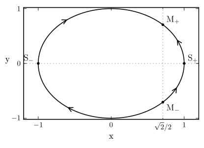
Figure 1: Phase space for the planar system of Eqs. (10) and (11). The critical points are indicated by $M_{\pm}$, for a scalar field with a matter-type effective EoS, and $S_{\pm}$ for a stiff-matter one. For $y<0$ we have the contracting phase and for $y>0$ the expanding phase. Lower and upper quadrants are not physically connected, because there is no classical mechanism that could drive a bounce between the contracting and expanding phases.

It will be useful to analyze what happens with $H$ and $\dot{\phi}$ when the system is close to the critical points $S_{\pm}$. Around these points, we get from Eq. (12) that

$$H\propto\mathrm{e}^{-3\alpha},$$ (16)

as it is expected for a stiff-like fluid, which diverges when approaching the singularity. Consequently, using Eq. (8) we deduce that in the neighborhood of these points the asymptotic behavior is

$$\lim_{x\to\pm 1}\left\{\begin{array}[]{c l l}H&\to-\infty,\\ \phi&\to\pm\frac{\sqrt{6}}{\kappa}\alpha&\to\mp\infty,\\ \dot{\phi}&\to\pm\frac{\sqrt{6}}{\kappa}H&\to\mp\infty,\end{array}\right.$$ (17)

in the contracting phase, while in the expanding phase one gets

$$\lim_{x\to\pm 1}\left\{\begin{array}[]{c l l}H&\to\infty,\\ \phi&\to\pm\frac{\sqrt{6}}{\kappa}\alpha&\to\mp\infty,\\ \dot{\phi}&\to\pm\frac{\sqrt{6}}{\kappa}H&\to\pm\infty.\end{array}\right.$$ (18)

Figure 2 summarizes what we presented above qualitatively. Nevertheless, this figure represents only the critical points and flow resulting from the classical equations of motion. The quantum dynamics takes place in the portion of phase space where the Ricci scalar is close to the Planck length, near the singularities. As in Fig. 2 we set $\kappa=\sqrt{6}$, the $S_{\pm}$ critical points representing the classical singularities are depicted in this figure by the lines $H=\pm\dot{\phi}$ when $|H|\to\infty$ and $|\dot{\phi}|\to\infty$. Hence, quantum effects can modify Fig. 2 only around these regions, with a quantum bounce connecting the regions around $S_{\pm}$ in the lower quadrants to the regions around $S_{\pm}$ in the upper quadrants. However, trajectories connecting the neighborhood of $S_{+}$ in the lower quadrant to the neighborhood of $S_{+}$ in the upper quadrant, or similarly connecting the neighborhoods of $S_{-}$ in both quadrants, necessarily cross the classical $M_{\pm}$ line, $H=\sqrt{2}\dot{\phi}$. As we will see, in the de Broglie-Bohm quantum theory, which we will use in this paper, velocity fields yielding the quantum Bohmian trajectories are single valued functions on phase space, as they arise from well defined functions on this space (the phase’s gradient from the corresponding Wheeler-DeWitt wave equation’s solution). Consequently, such trajectories cannot cross each other. Hence, the only way to connect the almost singular contracting and expanding behaviors without crossing the line $M_{\pm}$ is through a connection from the regions around $S_{\pm}$ to the regions around $S_{\mp}$, in this reversed order, necessarily. Indeed, as we will see below [see Eq. (28)], around the critical points $S_{\pm}$ the quantum bouncing trajectories have a well defined sign for $\dot{\phi}$, which is determined completely from the model parameters. As $H$ necessarily changes sign through a bounce, then these bouncing trajectories can only connect the neighborhoods of $S_{\pm}$ to the ones of $S_{\mp}$. Concluding, there is no solution in the complete phase space where the Universe contracts in the direction of $S_{-}$ ($S_{+}$) and expands from $S_{-}$ ($S_{+}$). A bounce is only possible in the phase space of $H$ and $\dot{\phi}$ if it connects the contracting phase ending in $S_{+}$ ($S_{-}$) to the expansion starting from $S_{-}$ ($S_{+}$).

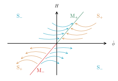
Figure 2: This qualitative figure illustrates the behavior of the solutions for $H$ and $\dot{\phi}$ close to the critical points of the classical model Eqs. (10) and (11). In this figure we chose $\kappa=\sqrt{6}$, hence the $M_{\pm}$ critical points are represented by the line $H=\sqrt{2}\dot{\phi}$, while the $S_{\pm}$ critical points are represented by the lines $H=\pm\dot{\phi}$ for $|H|\to\infty$ and $|\phi|\to\infty$. In a full quantized system, in which the Universe bounces due to the quantum corrections close to the Planck scale, the allowed phase space should connect the contraction finishing in $S_{\pm}$ with the expansion beginning in $S_{\mp}$.

For the model in consideration, we have then two possible histories of the Universe, depicted in Figs. 3 and 4. In the case of Fig. 3, a contracting phase starts close to $M_{-}$ (matter-fluid era), passes through a DE phase and ends in $S_{-}$ [as described in Eq. (15)], where the scalar field behaves as an stiff-matter fluid. At this point, new physics takes place performing a bounce and the Universe starts expanding from $S_{+}$ (scalar field as stiff-matter) and ends in matter-like expansion in $M_{+}$. There is no DE epoch in the expanding phase in this scenario.

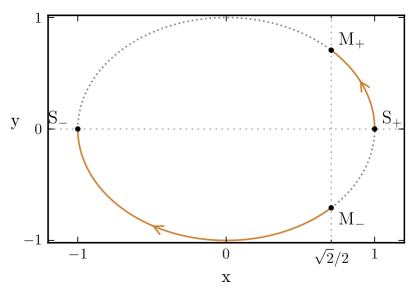
Figure 3: Case A: the scalar field has a DE-type equation of state during contraction. By means of the quantum bounce, this system can not address the DE in the future, since the matter attractor is reached before.

The case of Fig. 4 goes in the opposite direction. Contraction happens from a matter epoch, $M_{-}$, to a stiff-matter one, $S_{+}$. The new physics avoids the singularity and brings the Universe to an expansion that starts in $S_{-}$ followed by a DE epoch, ending finally in $M_{+}$, a matter-like epoch.

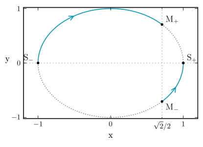
Figure 4: Case B: the contracting phase begins close to the unstable point $M_{-}$, in which the scalar field has a dust-type EoS. After the quantum bounce, the system emerges from $S_{-}$ and follows a DE phase until reaches the future attractor $M_{+}$.

The two above-mentioned scenarios have the interesting feature of a transient DE-like phase. For the sake of future reference along the article, let us call the case with DE during contraction, Fig. 3, case A, and the one with DE during expansion, Fig. 4, case B.

Case A shows the less compelling situation, where the background performs a matter contraction followed by a DE epoch before the bounce, but the expanding phase has no DE epoch. Previous works considering the presence of DE during contraction used a ghost field to perform the bounce. In such scenarios the phase space is very different from the one presented here, and it can have a DE epoch in both contracting and expanding phases Heard and Wands (2002); Cai et al. (2016). Nevertheless, a complete and rigorous calculation of the primordial power spectra in such scenarios have not yet been performed.

Case B is the one we will explore in this work. As we will see, the same scalar field with exponential potential that realizes the matter bounce scenario yielding an adiabatic scale invariant power spectrum also produces a DE epoch in the expanding phase. Furthermore, there is no need of an extra ghost potential nor any auxiliary scalar fields in order to yield the physical conditions that produce the bounce.

As we mentioned earlier, there is no classical bounce in the previous described backgrounds. Close to the attractor of the contracting phase, $S_{+}$ in case A and $S_{-}$ in case B, $H\propto-a^{-3}$, and when $a\rightarrow 0$ we reach a singularity. This happens because the kinetic term dominates the Lagrangian of the scalar field and diverges, but in these cases it has already been proved that quantum bounce solutions may arise. In the next section we present the results from Colistete et al. (2000), and show how they can by applied to our case to avoid the singularity.

III The quantum bounce

Quantum cosmology is the field of research in which quantum theory is applied to the Universe, and should have the standard cosmological model as its classical limit. This interesting and challenging topic, not only whitens fundamental problems of cosmology, as the singularity problem, but also allows fundamental quantum mechanics to be tested at the cosmological level Calcagni (2013); Peter et al. (2005); Martin et al. (2012); Underwood and Valentini (2016); Benetti et al. (2016).

The quantum description of gravity, besides facing many difficulties with the non-renormalizable aspect of GR Shomer (2007), also suffer from fundamental conceptual issues in what concerns the application of a quantum theory to the description of the whole Universe. In order to construct a quantum theory for the Universe, the traditional Copenhagen interpretation of quantum mechanics has to be replaced. Its main limitation is the postulate of the collapse of the wave function Wiltshire (1995); Pinto-Neto and Fabris (2013), where an outside classical system is necessary to perform the collapse. This does not make sense if the whole Universe is quantized.

The quantum theory which will replace the traditional Copenhagen point of view must of course be able to reproduce the results of quantum experiments already performed, but it must also dispense this exterior classical world, or collapse recipes, in order to be applicable to quantum cosmology. There are many proposals of quantum theories that satisfy these criteria, and were already applied to Cosmology: the consistent histories approach Griffiths (1984); Zurek (1990); Omnès (1994); Bom et al. (2014), collapse models for the wave-function Pearle (1976); Ghirardi et al. (1987); Underwood and Valentini (2016); Benetti et al. (2016), the many worlds interpretation Everett (1957); DeWitt and Graham (1973); Page (1999), and the dBB quantum theory Bohm and Hiley (1993); Holland (1993); Pinto-Neto and Fabris (2013), which is the one we will adopt here.

The canonical quantization of gravity obtained through the ADM formalism Arnowitt et al. (2008); DeWitt (1967), which should be an effective limit of a more fundamental theory, can be interpreted using the dBB formulation of quantum mechanics. The dynamics of the wave function of the Universe is given by the Wheeler-DeWitt equation from where, in this formulation, one can obtain Bohmian trajectories with objective reality describing the evolution of the whole system. In this approach, there is no need to postulate any collapse of the wave function of the Universe Pinto-Neto (2005); Pinto-Neto and Fabris (2013).

Both models described in this paper depicted in Figs. 3 and 4 present the same feature: the end of the classical contraction and the beginning of classical expansion happen when the kinetic energy overcomes the scalar field potential $V(\phi)$. A system consisting of a flat, homogeneous and isotropic space-time in the presence of a scalar-field with a dominant kinetic term has already been quantized. The Bohmian trajectories resulting from the Gaussian superposition of plane wave functions led to bounce solutions. Details of this construction can be found in Colistete et al. (2000). We will summarize their results in what follows.

In the case where the dynamics is dominated by the kinetic term, the Hamiltonian for a scalar field in the metric (3) reads

$$H=N{\mathcal{H}}=\frac{N\kappa^{2}}{12V\mathrm{e}^{3\alpha}}\left(-\Pi_{\alpha}^{2}+\Pi_{\phi}^{2}\right),$$ (19)

where $V$ is the volume of the conformal hypersurface, and from here on we will be using the dimensionless scalar field

$$\phi\rightarrow\frac{\kappa\phi}{\sqrt{6}}.$$

The associated momenta to the canonical variables $\alpha$ and $\phi$ are, respectively,

$$\Pi_{\alpha}=-\frac{6V}{N\kappa^{2}}\mathrm{e}^{3\alpha}\dot{\alpha},\qquad\Pi_{\phi}=\frac{6V}{N\kappa^{2}}\mathrm{e}^{3\alpha}\dot{\phi}.$$ (20)

Finally, we choose the conformal hypersurface volume as $V=4\pi\ell_{{}_{\mathrm{P}}}^{3}/3$, where $\ell_{{}_{\mathrm{P}}}\equiv\sqrt{G_{{}_{\mathrm{N}}}}=1/(\sqrt{8\pi}M_{{}_{\mathrm{P}}})$ is the Planck length. With this choice, the scale factor value has an absolute meaning, i.e., when $a=1$ the Universe has approximately the Planck volume.

Performing the Dirac quantization procedure, we can write the Wheeler-DeWitt equation as

$${\hat{{\mathcal{H}}}}\Psi(\alpha,\phi)=0\Rightarrow\left[-\frac{\partial^{2}}{\partial\alpha^{2}}+\frac{\partial^{2}}{\partial\phi}\right]\Psi(\alpha,\phi)=0.$$ (21)

The general solution is

$$\Psi(\alpha,\phi) =F(\phi+\alpha)+G(\phi-\alpha)$$

$$\equiv\int\mathrm{d}k\Big{\{}f(k)\exp\left[ik(\phi+\alpha)\right]+$$ (22)

$$\qquad\qquad g(k)\exp\left[ik(\phi-\alpha)\right]\Big{\}},$$

where $f$ and $g$ are arbitrary functions of $k$.

Writing the wave-function in polar form, $\Psi=R\exp(iS)$, where $R$ is the amplitude and $S$ is the phase in units of $\hbar$, and substituting into Eq. (21) leads to the Hamilton-Jacobi like equation for the phase $S$,

$$\left(\frac{\partial S}{\partial\alpha}\right)^{2}-\left(\frac{\partial S}{\partial\phi}\right)^{2}-\frac{1}{R}\left(\frac{\partial^{2}R}{\partial\alpha^{2}}-\frac{\partial^{2}R}{\partial\phi}\right)=0.$$ (23)

When the last term of Eq. (23), the so called quantum potential, is negligible with respect to the others, we get the usual classical Hamilton-Jacobi equation for the minisuperspace model at hand. Assuming the ontology of the trajectories $\alpha(t)$ and $\phi(t)$, this classical limit suggests the imposition of the so called dBB guidance relations in order to determine the trajectories, in correspondence to the usual classical Hamilton-Jacobi theory, and they read, in cosmic time $N=1$,

$$\Pi_{\alpha} =\frac{\partial S}{\partial\alpha}=-\ell_{{}_{\mathrm{P}}}\mathrm{e}^{3\alpha}\dot{\alpha},$$ (24)

$$\Pi_{\phi} =\frac{\partial S}{\partial\phi}=\ell_{{}_{\mathrm{P}}}\mathrm{e}^{3\alpha}\dot{\phi}.$$ (25)

When the quantum potential is not negligible in Eq. (23), these Bohmian quantum trajectories may be different from the classical ones, and may present a bounce.

In Ref. Colistete et al. (2000) it was chosen the simple appealing prescription of a Gaussian superposition of plane waves in Eq. (22) given by

$$f(k)=g(k)=\exp\left[\frac{-(k-d)^{2}}{\sigma^{2}}\right].$$ (26)

Calculating the phase $S$ of the aforementioned solution, and substituting it into the guidance relations (24) and (25), we find the planar system that describes the Bohmian trajectories

$$\ell_{{}_{\mathrm{P}}}\dot{\alpha} =\frac{\phi\sigma^{2}\sin(2d\alpha)+2d\sinh(\sigma^{2}\alpha\phi)}{2\mathrm{e}^{3\alpha}\left[\cos(2d\alpha)+\cosh(\sigma^{2}\alpha\phi)\right]},$$ (27)

$$\ell_{{}_{\mathrm{P}}}\dot{\phi} =\frac{-\alpha\sigma^{2}\sin(2d\alpha)+2d\cos(2d\alpha)+2d\cosh(\sigma^{2}\alpha\phi)}{2\mathrm{e}^{3\alpha}\left[\cos(2d\alpha)+\cosh(\sigma^{2}\alpha\phi)\right]}.$$ (28)

When solving the equations above we have a time definition in units of Planck time (essentially putting $\ell_{{}_{\mathrm{P}}}=1$ in the above equations). However, since the scales of interest for the perturbations are those around the Hubble radius today, $R_{H}\equiv 1/H_{0}$ (here we adopt the current value $H_{0}=67.8\pm 0.9\;\mathrm{km}\;\mathrm{s}^{-1}\mathrm{Mpc}^{-1}$ Planck Collaboration et al. (2015a)), we convert back using the factor $R_{H}/\ell_{{}_{\mathrm{P}}}$ when matching with the classical solution.

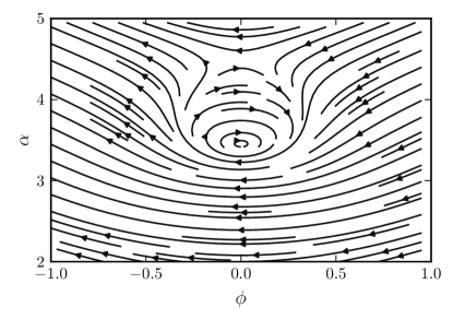
Figure 5: Phase space for the system of Eqs.(27) and (28) for $d=-1$ and $\sigma=1$. We can notice bouncing and cyclic solutions. The bounces in the figure correspond to case B, where $\dot{\phi}<0$, and it connects regions around $S_{+}$ in the contracting phase with regions around $S_{-}$ in the expanding phase.

In Fig. 5 we have the phase space for Eqs. (27) and (28). We can notice the presence of bounce and cyclic solutions. It is easy to calculate the nodes and the centers. They happen all along the line $\phi=0$: the nodes for $d\alpha=(2n+1)\pi/2$ and the centers for $\sigma^{2}\alpha/2d=\cot(d\alpha)$.

The classical limits of Eqs. (27) and (28) are obtained for large $\alpha$, when the hyperbolic function dominates. From the definition of $x$ in that limit, it is straightforward to obtain the relations

$$x \approx\coth\left(\sigma^{2}\alpha\phi\right),$$ (29)

$$\frac{H}{H_{0}} \approx\frac{R_{H}}{\ell_{{}_{\mathrm{P}}}}\frac{d\mathrm{e}^{-3\alpha}}{x},$$ (30)

$$\ell_{{}_{\mathrm{P}}}\dot{\phi} \approx d\mathrm{e}^{-3\alpha}.$$ (31)

These equations imply that $\phi$ and $x$ have the same sign, and $\dot{\phi}$ the same sign as $d$ in the classical limit. This means that in case A, since its contraction ends in $x\to-1$, Eq. (30) is satisfied only if $d>0$. Similarly, case B requires $d<0$. This result is consistent with our discussion in Sec. II. In case A, the quantum dynamics starts with $x\approx-1$ ($\phi\ll-1$), ending in $x\approx 1$ ($\phi\gg 1$). The opposite happens in case B, i.e., our bouncing dynamics always connects the classical critical points $S_{-}$ ($S_{+}$) with $S_{+}$ ($S_{-}$). In practice, the sign of $d$ determines which case is being evolved.

IV Matching of background

In the previous section we presented the quantum corrections to the system when the kinetic term of the scalar field dominates, yielding a bounce. In order to construct a complete background, we should be able to match the solutions from the classical evolution, described in Sec. II with the quantum solution from the system of Eqs. (27) and (28).

In a complete formulation of this problem, the designation of “classical” and “quantum” solutions should not be taken strictly. In the complete dBB formulation, we have the Bohmian trajectories that accounts for both regimes. In our hybrid background, we make this distinction only to emphasize the fact that we do not have a complete Bohmian trajectory and to make explicit which equations of motion are being used. The full quantum description of this system can be found in Ref. Colin and Pinto-Neto (2017), where full Bohmian bounce solutions are exhibited. However, to perform the calculation of cosmological perturbations around some full Bohmian trajectory is quite cumbersome, hence we prefer to adopt this simpler method of matching classical to quantum solutions, with no loss of relevant information.

The nomenclature in what follows may be tricky, and in order to avoid confusion we will adopt the expressions quantum/classical solutions, regimes or branches to distinguish the dynamics described by Eqs. (27) and (28) (quantum) from the one determined by Eqs. (10) and (11) (classical). To make reference to the period at which the quantum potential is relevant, we will adopt quantum phase in opposition to classical phase, in which the quantum potential is irrelevant.

The complete background solution has three branches. The first one is the classical contraction that starts with $x\approx 1/\sqrt{2}$ and ends in $x\rightarrow\pm 1$. The second branch is the quantum background that starts in $x\approx\pm 1$ and bounces to $x\to\mp 1$. The third branch, the classical expansion, starts with $x\approx\mp 1$ and ends with $x\rightarrow 1/\sqrt{2}$. The lower signs stand for case A while the upper signs for the case B. The matching is performed guaranteeing continuity of the solutions up to the first derivative at the time when they move from the quantum to the classical regimes. This happens when the quantum solutions reach their classical limit given in Eqs. (29) and (30).

However, the classical limit of the quantum regime happens when $x=\pm 1$, which is a critical point of the classical equations, Eqs. (10) and (11). To start the classical phase exactly in a critical point means that the Universe would be stuck in the stiff-matter epoch. Nonetheless, the initial classical epoch is unstable, hence we always start it with a small shift around the critical points. We will parametrize $x$ in the proximity of the stiff critical points by $x=\pm(1-\epsilon_{\pm})$, $0<\epsilon_{\pm}\ll 1$. In the matching point, $\epsilon_{\pm}$ should be small enough to justify the classical limit of the quantum regime.

If we had a complete Bohmian trajectory, it would only be necessary to set initial conditions in the far past. For instance, we would give an initial $x_{\lambda}$ close to the unstable point $M_{-}$. The proximity to the critical point and from which side of the critical point it begins dictates the duration of the matter contraction and selects between cases A and B (which must be compatible with the choice of sign for $d$). We would also give an initial scale factor, $a_{\mathrm{ini}}$, and a Hubble constant, $H_{\mathrm{ini}}$, ($\phi_{\mathrm{ini}}$ and $\dot{\phi}_{\mathrm{ini}}$ are constrained by the value of $x_{\mathrm{ini}}$ and $V_{0}$ through the Friedmann equation). With that all set, the Bohmian trajectories would handle the whole evolution until the expanding phase. Naturally, parameters as the minimum scale factor at the bounce, the energy scale of the DE epoch, and the duration of the quantum bounce would be obtainable from the model parameter $V_{0}$, the system wave-function and the initial conditions.

Because of our matching procedure, things are not so simple. We have not only the choice of initial conditions and the quantum bounce parameters, $d$ and $\sigma$ (extracted from the wave-function), but also two new variables, namely, the contraction and expansion matching parameters, denoted by $\epsilon_{c}$ and $\epsilon_{e}$, respectively. In what follows, we will rewrite these two variables in terms of new parameters which also controls the number of e-folds between the bounce and a given Hubble scale.

In order to connect the classical solution parameters at the matching point with its quantum evolution, we integrate Eqs. (12) and (13) analytically. However, it is not possible to write explicit functions for $x(\alpha)$ and $H(\alpha)$. The best we can do is to obtain implicit functions which, apart from two integration constants, read

$$3\alpha =-\sqrt{2}\tanh^{-1}(x)-\ln\left[\frac{\left(\frac{1}{\sqrt{2}}-x\right)^{2}}{1-x^{2}}\right]+\mathrm{cte},$$ (32)

$$\ln{}H =\sqrt{2}\tanh^{-1}(x)+\ \ln\left(\frac{\frac{1}{\sqrt{2}}-x}{1-x^{2}}\right)+\mathrm{cte}.$$ (33)

We begin by recasting these solutions in a more convenient form

$$\left(\frac{a}{{\bar{a}}_{0}}\right)^{6}\left(\frac{H}{H_{0}}\right)^{2} =\frac{C_{1}}{\left(\frac{1}{\sqrt{2}}-x\right)^{2}},$$ (34)

$$\left(\frac{a}{{\bar{a}}_{0}}\right)^{3} =\frac{C_{2}\left(1-x\right)^{\gamma_{+}}\left(1+x\right)^{\gamma_{-}}}{\left(\frac{1}{\sqrt{2}}-x\right)^{2}},$$ (35)

where $\gamma_{\pm}\equiv 1\pm\frac{1}{\sqrt{2}}$, and $C_{1}$ and $C_{2}$ are constants. We introduced $H_{0}$, the Hubble parameter today, and ${\bar{a}}_{0}$ for mere convenience. Note that these constants can be absorbed in $C_{1}$ and $C_{2}$, and they do not represent any additional freedom of the system. We can calculate the number of e-folds between the critical points $S_{\pm}$ and $M_{\pm}$. Expanding Eq. (35) around $x=\pm(1-\epsilon_{\pm})$ and $x=(1/\sqrt{2}\pm\epsilon_{\lambda})$ at leading order, yields, respectively

$$\left(\frac{a_{\pm}}{{\bar{a}}_{0}}\right)^{3} \approx\frac{C_{2}2^{\gamma_{\mp}}\epsilon_{\pm}^{\gamma_{\pm}}}{\gamma_{\mp}^{2}},$$ (36)

$$\left(\frac{a_{\lambda}}{{\bar{a}}_{0}}\right)^{3} \approx\frac{C_{2}\gamma_{-}^{\gamma_{+}}\gamma_{+}^{\gamma_{-}}}{\epsilon_{\lambda}^{2}},$$ (37)

where we note that, at leading order, the second expression does not depend from which side we approach $M_{\pm}$. From their ratio we get

$$\left(\frac{a_{\pm}}{a_{\lambda}}\right)^{3}\approx\frac{2^{\gamma_{\pm}}}{\gamma_{-}^{\gamma_{+}}\gamma_{+}^{\gamma_{-}}\gamma_{\mp}^{2}}\epsilon_{\pm}^{\gamma_{\pm}}\epsilon_{\lambda}^{2}.$$ (38)

Imposing that we must be close enough to the critical points, i.e., $\epsilon_{i}<10^{-4}$ (for $i=\pm,\;\lambda$), Eq. (38) leads to

$$\frac{a_{+}}{a_{\lambda}}\lesssim\mathrm{e}^{-10},\qquad\frac{a_{-}}{a_{\lambda}}\lesssim\mathrm{e}^{-6}.$$

This means that the trajectories $M_{-}\to S_{-}$ or $S_{-}\to M_{+}$, depicted in the lower quadrants of Fig. 3 and the upper quadrants of Fig. 4, respectively, must have a minimum of $6$ e-folds. The remaining trajectories ($M_{-}\to S_{+}$ and $S_{+}\to M_{+}$) must have a minimum of $10$ e-folds.

Analogously, we can also calculate the number of e-folds until the DE phase ($x=0$), yielding

$$\left(\frac{{a_{\mathrm{de}}}}{{\bar{a}}_{0}}\right)^{3}\approx 2C_{2},\quad\left(\frac{a_{-}}{{a_{\mathrm{de}}}}\right)^{3}\approx\frac{2^{\gamma_{+}}\epsilon_{-}^{\gamma_{-}}}{2\gamma_{+}^{2}},\quad\frac{a_{-}}{{a_{\mathrm{de}}}}\lesssim\mathrm{e}^{-1}.$$

The background will be constructed numerically from the quantum bounce to the classical contracting and expanding phases. As the solutions are necessarily asymmetric, the matching between the quantum and classical regimes can be arranged in two possible ways, depending on whether we want to write $\epsilon_{c}$ and $\epsilon_{e}$ in terms of the number of e-folds between the bounce and a point in the matter-fluid domination or the DE phase. Let us now describe this construction in the following sub-sections.

IV.1 Initial conditions at the bounce

Our numerical calculation consists in solving the background, starting from the bounce and evolving to the expanding and contracting phases. In order to accomplish this, we start the calculation around the bounce with slightly positive (negative) time for the expansion (contraction) phase. A convenient time variable is $\tau$ defined by

$$\alpha=\alpha_{\mathrm{b}}+\frac{\tau^{2}}{2},$$ (39)

which leads to $\mathrm{d}\tau/\mathrm{d}t=H/\tau$ and $\mathrm{d}\alpha=\tau\mathrm{d}\tau$. We have already included in this choice of time variable the initial condition for $\alpha$, i.e., we always set the bounce at $\tau=0$. We can see from Eq. (27) that the initial value $\alpha(t_{0})=0$ induces a trivial solution $\alpha(t)=0$. As trajectories in the $(\alpha,\phi)$ plane cannot cross, this implies that $\alpha$ cannot chance sign along the possible trajectories. Hence, the choice of time above select the positive branch of the phase space $(\alpha,\phi)$, Fig. 5. For a single bounce, $\alpha$ attains its smallest value at the bounce, which provides the last justification for our parametrization (39).

We need now the initial condition for the field $\phi$. Examining Eq. (27), we realize that the bounce can only take place when $\phi=0$. Indeed, the denominator is always positive, and it diverges to the classical limit, where no bounce is possible. Hence the necessary condition for the bounce $\dot{\alpha}=0$ can occur if and only if the numerator is zero. If there were a root of the numerator of Eq. (27) different from the trivial one $\phi=0$, it would satisfy

$$\frac{\sinh(A)}{A}=-\frac{\sin(B)}{B},$$

where we have defined $A=\sigma^{2}\alpha\phi$ and $B=2d\alpha$, both different from zero, by assumption. However, this equation cannot be solved for any real $A$ and $B$. Therefore, for the quantum system, we will always use the only possible initial conditions $\alpha(0)=\alpha_{\mathrm{b}}$ and $\phi(0)=0$.

Expanding Eqs. (27) and Eq. (28) about the bounce, we get the leading order approximations

$$\frac{\mathrm{d}\tau}{\mathrm{d}t_{Q}}=\frac{\phi}{\tau}D_{1},$$ (40)

$$\frac{\mathrm{d}\phi}{\mathrm{d}t_{Q}}=D_{2},$$ (41)

where we rewrote the equation in terms of $\tau$ and the convenient dimensionless time variable $\mathrm{e}^{3\alpha}\ell_{{}_{\mathrm{P}}}\mathrm{d}t_{Q}=\mathrm{d}t$. The two constants $D_{1}$ and $D_{2}$ are

$$D_{1} =\frac{\sigma^{2}\left[\sin(2d\alpha_{\mathrm{b}})+2d\alpha_{\mathrm{b}}\right]}{2\left[2\cos(2d\alpha_{\mathrm{b}})+1\right]},$$

$$D_{2} =\frac{-\alpha_{\mathrm{b}}\sigma^{2}\sin(2d\alpha_{\mathrm{b}})+2d\cos(2d\alpha_{\mathrm{b}})+2d}{2\left[2\cos(2d\alpha_{\mathrm{b}})+1\right]}.$$

These equations can be easily integrated to give

$$\tau=t_{Q}\sqrt{D_{1}D_{2}},\qquad\phi=t_{Q}D_{2},$$ (42)

where we have also chosen the sign of $\tau$ coinciding with the sign of $t_{Q}$. These solutions hold close to the bounce, hence we chose a very small value of $t_{Q}$, for instance $t_{Q}^{\mathrm{ini}}\propto\pm\mathcal{O}(10^{-50})$, to start the numerical evolution of Eqs. (27) and (28), using the new time $t_{Q}$. In order to do that, one must know $D_{1}$ and $D_{2}$, hence $\alpha_{b},d,\sigma$ must be given. The above choice of initial $t_{Q}$ gives well defined numerical results for the whole range of parameters studied in this work. The time variable $t_{Q}$ is then used to solve the quantum dynamics until the matching with the classical phases, in the contracting branch and in the expanding branch. For $d<0$, the positive time direction in the integration moves the solution to the DE branch, while for $d>0$, the positive time direction moves the solution to the branch without DE. From there on, we have two possibilities to parametrize the matching, depending on whether there is a DE behavior in the classical dynamics or not.

IV.2 Matching with matter domination scale

Evolving the quantum era as described above, we arrive at a nearly classical evolution with stiff matter behavior at some $a_{\pm}=\ln(\alpha_{\pm})$ with $x(a_{\pm})=\pm[1-\epsilon_{\pm}(a_{\pm})]$. At this point, we match the quantum evolution with the classical one. In order to control this matching and its cosmological meaning, we will write $a_{\pm}$ and its corresponding $\epsilon_{\pm}(a_{\pm})$ in terms of the number of e-folds between the bounce and the matter-fluid domination, where $x=1/\sqrt{2}+\epsilon_{\lambda}$, with $0<\epsilon_{\lambda}\ll 1$. We will suppose that the free constant $\bar{a}_{0}$ belongs to the infinity open set of real numbers satisfying $x(\bar{a}_{0})=1/\sqrt{2}+\epsilon_{\lambda}(\bar{a}_{0})$, with $0<\epsilon_{\lambda}(\bar{a}_{0})\ll 1$.

The first step is to impose continuity of the Hubble function at the matching point. Expanding Eq. (34) about $x_{\pm}$ gives

$$\left(\frac{H_{\pm}}{H_{0}}\right)^{2}\approx\frac{C_{1}}{\gamma_{\mp}^{2}}\left(\frac{{\bar{a}}_{0}}{a_{\pm}}\right)^{6}.$$ (43)

Equating this expression to Eq. (30) yields

$$C_{1}=\frac{R_{H}^{2}}{\ell_{{}_{\mathrm{P}}}^{2}}\frac{d^{2}\gamma_{\mp}^{2}}{\bar{a}_{0}^{6}}.$$ (44)

This equation relates the free constant $C_{1}$ of the classical system to $\bar{a}_{0}$. As the scale factor at the bounce $a_{b}$ was already chosen, giving the physical parameter

$$\mathcal{X}_{\mathrm{b}}\equiv\frac{{\bar{a}}_{0}}{a_{\mathrm{b}}},$$ (45)

is equivalent to fixing $C_{1}$. The parameter $\mathcal{X}_{\mathrm{b}}$ yields the number of e-folds from the bounce to the moment of the matter-fluid domination determined by $\bar{a}_{0}$, which, as commented above, is still rather arbitrary: the only constraint on it is to satisfy $x(\bar{a}_{0})=1/\sqrt{2}+\epsilon_{\lambda}(\bar{a}_{0})$, with $0<\epsilon_{\lambda}(\bar{a}_{0})\ll 1$.

For the second constant $C_{2}$, we obtain from Eq. (36) that

$$C_{2}=\frac{\gamma_{\mp}^{2}}{2^{\gamma_{\mp}}\epsilon_{\pm}^{\gamma_{\pm}}}\left(\frac{a_{\pm}}{{\bar{a}}_{0}}\right)^{3}.$$ (46)

This equation relates the matching point $a_{\pm}$ and its corresponding $\epsilon_{\pm}(a_{\pm})$ to $C_{2}$. Note, however, that the end of the quantum evolution does not designate any specific value of $a_{\pm}$ as long as the quantum evolution stays very close to the stiff matter classical evolution. Hence, all points where $0<\epsilon_{\pm}\ll 1$ are acceptable. Here lies the ambiguity of the matching.

We could arbitrarily choose $a_{\pm}$ in order to fix $C_{2}$. However, we will do the reverse: we will connect $C_{2}$ with sensible cosmological parameters associated with physical features of the classical branch, and after a judicious choice of them determining $C_{2}$, we use Eq. (46) to finally find the matching point $a_{\pm}$. This can be done as follows: close to the matter-fluid epoch, the zero order term of the Hubble function reads

$$\left(\frac{H}{H_{0}}\right)^{2}\approx\frac{C_{1}}{C_{2}\gamma_{-}^{\gamma_{+}}\gamma_{+}^{\gamma_{-}}}\left(\frac{{\bar{a}}_{0}}{a}\right)^{3}.$$ (47)

The above result motivates the definition of the arbitrary constant

$$\Omega_{d}=\frac{C_{1}}{C_{2}\gamma_{-}^{\gamma_{+}}\gamma_{+}^{\gamma_{-}}}=\frac{R_{H}^{2}}{\ell_{{}_{\mathrm{P}}}^{2}}\frac{d^{2}\gamma_{\mp}^{2}}{C_{2}\gamma_{-}^{\gamma_{+}}\gamma_{+}^{\gamma_{-}}\bar{a}_{0}^{6}}.$$ (48)

This constant is very useful, as long as it gives a precise meaning to $\mathcal{X}_{\mathrm{b}}$. Indeed, from Eq. (47) and Eq. (48), we get

$$H^{2}(a={\bar{a}}_{0})\approx H_{0}^{2}\Omega_{d}.$$

The parameter $\mathcal{X}_{\mathrm{b}}$ can now be understood as yielding the number of e-folds between the bounce and the moment where the Hubble radius is $R_{H}/\sqrt{\Omega_{d}}$. Hence, once $\Omega_{d}$ is given, $\mathcal{X}_{\mathrm{b}}$ acquires a very precise meaning.

In terms of the physical variables $\Omega_{d}$ and $\mathcal{X}_{\mathrm{b}}$, the constant $C_{2}$ reads,

$$C_{2}=\frac{R_{H}^{2}}{\ell_{{}_{\mathrm{P}}}^{2}}\frac{d^{2}\gamma_{\mp}^{2}}{\Omega_{d}\gamma_{-}^{\gamma_{+}}\gamma_{+}^{\gamma_{-}}a_{\mathrm{b}}^{6}\mathcal{X}_{\mathrm{b}}^{6}}.$$ (49)

This expression is completely determined by our choices of quantum initial condition $a_{b}$ and the constants $\Omega_{d}$ and $\mathcal{X}_{\mathrm{b}}$. Plugging it into Eq. (46), we obtain our matching time

$$\frac{a_{\pm}}{\epsilon_{\pm}^{\gamma_{\pm}/3}}\approx\frac{1}{\mathcal{X}_{\mathrm{b}}a_{\mathrm{b}}}\left(\frac{R_{H}^{2}d^{2}2^{\gamma_{\mp}}}{\ell_{{}_{\mathrm{P}}}^{2}\gamma_{-}^{\gamma_{+}}\gamma_{+}^{\gamma_{-}}\Omega_{d}}\right)^{1/3}.$$ (50)

Then, given a value for $\mathcal{X}_{\mathrm{b}}$ and $\Omega_{d}$, with the cosmological meanings described above, we must evolve the quantum branch until some values of $\alpha_{\pm}=\ln a_{\pm}$ and $\epsilon_{\pm}$ where Eq. (50) is satisfied. From this point on, we continue using the classical equations (13) with these matching values for $\alpha_{\pm}$ and $x_{\pm}$ as initial conditions.

Summarizing, from the classical dynamics we introduced four (redundant) constants to control the initial conditions $({\bar{a}}_{0},\;H_{0},\;C_{1},\;C_{2})$. We chose $H_{0}$ to match today’s value of the Hubble parameter in order to have the problem scaled to the perturbation scales of cosmological interest. To fix the other arbitrary parameters, we studied the classical solution around the matter-fluid critical point, introducing the matter parameter $\Omega_{d}$, which only serves to give a meaning to $\mathcal{X}_{\mathrm{b}}$. Note that the matching (50) depends only on the product $\mathcal{X}_{\mathrm{b}}^{3}\Omega_{d}$, evincing that one of these parameters is arbitrary. The first actual initial condition we impose by matching the value of the Hubble function in the end of a quantum branch with its value in the beginning of a classical branch. The second initial condition is, however, not completely determined by the quantum phase, as we can choose any small value of $\epsilon_{\pm}$ as we want. For this reason, we choose a value for $\mathcal{X}_{\mathrm{b}}$ (keeping $\Omega_{d}$ fixed), which has a clear cosmological meaning, to completely determine $a_{\pm}$ and $\epsilon_{\pm}$ through Eq. (50), and the subsequent system evolution .

Finally, it is useful to study the allowed values for $\mathcal{X}_{\mathrm{b}}$. Using for the moment $\Omega_{d}=1$, i.e., choosing $\mathcal{X}_{\mathrm{b}}$ to represent the number of e-folds between the bounce and the instant where the Hubble radius matches today’s value, we get

$$\mathcal{X}_{\mathrm{b}}\approx(a_{b}a_{\pm})^{-1}\left(\frac{R_{H}^{2}d^{2}2^{\gamma_{\mp}}\epsilon_{\pm}^{\gamma_{\pm}}}{\ell_{{}_{\mathrm{P}}}^{2}\gamma_{-}^{\gamma_{+}}\gamma_{+}^{\gamma_{-}}}\right)^{1/3}.$$ (51)

The value of $\mathcal{X}_{\mathrm{b}}$ is inversely proportional to $a_{b}a_{\pm}$, thus, to maximize $\mathcal{X}_{\mathrm{b}}$ we need to minimize $a_{b}a_{\pm}$. Using the fact that $\alpha_{b}>0$, we get $a_{b}=1$ as the minimum value of $a_{b}$. Assuming that the quantum phase is fast enough so that it has approximately zero e-folds of duration, we get $a_{\pm}=1$ as the minimum value of $a_{\pm}$. Then, ignoring the order one factors we get

$$\mathcal{X}_{\mathrm{b}}\lesssim 10^{40}d^{2/3}\epsilon_{\pm}^{\gamma_{\pm}/3},$$ (52)

which shows, that given the value of $d$, we have a maximum for the number of e-folds. This fact is very relevant for the perturbations, since their amplitudes are determined partially by $\mathcal{X}_{\mathrm{b}}$. Note also that this kind of constraint is present in any matter bounce, and it can make difficult to generate enough amplitudes for the perturbations without approaching too much the Planck scale. Moreover, $\mathcal{X}_{\mathrm{b}}$ is proportional to $\epsilon_{\pm}^{\gamma_{\pm}}$, thus, a long quantum branch ($\epsilon_{\pm}^{\gamma_{\pm}}$ very small) results in a shallow bounce.

IV.3 Matching with the dark energy scale

For trajectories containing the DE epoch, we have an alternative way to give meaning for a reference scale. We can choose ${\bar{a}}_{0}$ to represent the exact point where $w=-1$, i.e., $x=0$. At this point we have

$$\left[\frac{H(a={\bar{a}}_{0})}{H_{0}}\right]^{2}=2C_{1}\equiv\Omega_{\Lambda},\qquad 2C_{2}=1,$$ (53)

where we have introduced the parameter $\Omega_{\Lambda}$ (in the same way and with similar characteristics to $\Omega_{d}$). There is an important distinction to make in comparison with the other case. Here, we are matching with a fixed point in time, whereas, in the last matter-fluid we can match to any time where $0<\epsilon_{\lambda}\ll 1$. For this reason, the value of $\Omega_{\Lambda}$ completely determines the matching and in this case $\mathcal{X}_{\mathrm{b}}$ is obtained from it. For $\Omega_{\Lambda}=1$, DE domination takes place around our present Hubble time.

Since we have fully determined $C_{1}$ and $C_{2}$ all we need to do is substitute them on Eqs. (44) and (46) from which we obtain the matching condition

$$\frac{a_{-}}{\epsilon_{-}^{\gamma_{-}/3}}\approx\left(\frac{R_{H}|d|2^{\gamma_{+}}}{\ell_{{}_{\mathrm{P}}}\sqrt{2\Omega_{\Lambda}}\gamma_{+}}\right)^{1/3},$$ (54)

where we specialized in the _- branch since it is the only one containing a DE phase. The number of e-folds in this case is given by the logarithm of

$$\mathcal{X}_{\mathrm{b}}\approx\frac{1}{a_{\mathrm{b}}}\left[\frac{2R_{H}^{2}\gamma_{+}^{2}d^{2}}{\ell_{{}_{\mathrm{P}}}^{2}\Omega_{\Lambda}}\right]^{{1}/{6}}.$$ (55)

It is worth noting that the number of e-folds between the bounce and the $|H|=H_{0}$ scale, assuming $\Omega_{\Lambda}=1$, is different for the different matching procedures, showing the asymmetry of the model. Note also that the main factor in determining $\mathcal{X}_{\mathrm{b}}$ in the matter-fluid matching is $(R_{H}/\ell_{{}_{\mathrm{P}}})^{2/3}$ while for the DE matching we have $(R_{H}/\ell_{{}_{\mathrm{P}}})^{1/3}$, i.e., the DE matching produces a smaller number of e-folds in the branch where it is applied. It is also clear from the equation above that larger (smaller) $\Omega_{\Lambda}$ results in fewer (more) e-folds between the DE phase and the bounce.

One last comment: when the DE phase happens during expansion (the case B) it is natural to use this procedure to match, using $\Omega_{\Lambda}\approx 1$, which guarantees us that we could model the current accelerated expansion using this field. However, if the DE phase happens during the contraction (case A), we do not have any reason to choose a priori a given scale to match.

IV.4 Summarizing the background reconstruction

As explained in this section, the numerical integration used to construct the background model is initiated at the bounce itself, using the quantum guidance equations. For that, one should give the values of $\alpha_{b}$, $d$ and $\sigma$. The system is evolved until reaching the classical limit, where it is matched with the classical evolution. This matching is controlled by the cosmological parameters $\Omega_{\Lambda}$ and $\mathcal{X}_{\mathrm{b}}$. In the branch with a DE phase, the quantum evolution is halted when Eq. (54) is satisfied, while in the branch without a DE phase the quantum dynamics is stopped when condition (50) is reached. This gives the values of $\alpha_{\pm}$ and $x_{\pm}$ to be used as initial conditions to the subsequent integration of the classical equations (13).

Hence, the complete collection of parameters needed to fix the background model is ($\alpha_{b}$, $d$, $\sigma$, $\Omega_{\Lambda}$, $\mathcal{X}_{\mathrm{b}}$), all of them with clear cosmological significance. For $d>0$ we have case A, and the DE phase is in the contracting phase, while for $d<0$ we are in case B, and the DE phase is in the expanding phase.

As a last remark, the classical branch could, in principle, be calculated using Eq. (13), and all other quantities are obtained by simple integrals of $x$. However, the variable $x$ is not well behaved numerically, for instance, to represent a point very close to $S_{+}$, say $x=1-10^{20}$, we would need at least a $20$ decimal digits floating point number, well beyond the default double precision (about $16$ decimal digits), present in today’s computers. To avoid this numerical pitfall, we make the following change of variables

$$x_{\pm}(q_{\pm})=\pm\left(1-\frac{\gamma_{\mp}q_{\pm}}{1+q_{\pm}}\right),$$ (56)

which maps the $x$ range $(\pm 1,1/\sqrt{2})$ into the numerically well defined interval $(0,\;\infty)$. For this reason we solve numerically Eq. (13) written in terms of $q_{\pm}$ for the paths ending/beginning on $S_{\pm}$.

V Numerical solutions for the background

In this section we will explore the parameter space of the theory, and see its influence in the complete background behavior, which will be used in the perturbative analysis. When one parameter is varied in the figures below, the bold values in Tab. 2 designate the other parameters which get fixed in the corresponding figures. For example, the different curves appearing in Fig. 7 for the case B corresponding to the different values of $d$ present in Tab. 2 were calculated with the parameters $\sigma=0.5$, $\alpha_{\mathrm{b}}=10^{-40}$, ${\mathcal{X}}_{\mathrm{b}}=10^{30}$ and $\Omega_{\Lambda}=1$. Also, since we are interested in perturbations at scales near the Hubble radius today, we from here on use $\Omega_{d}=1$.

$d$	$\sigma$	$\alpha_{\mathrm{b}}$	$\mathcal{X}_{\mathrm{b}}$	$\Omega_{\Lambda}$
$10^{-5}$	$5\times 10^{-2}$	$\mathbf{10^{-40}}$	$10^{20}$	$\mathbf{1}$
$\mathbf{10^{-1}}$	$\mathbf{5\times 10^{-1}}$	$10^{-5}$	$10^{25}$	$10^{20}$
$10$	$5$	$1$	$\mathbf{10^{30}}$	$10^{40}$

Table 2: The parameters of the numerical solutions, Figs. 7 to 10. The bold values in the table are fixed when one parameter is varied. In all examples we considered $\Omega_{d}=0.3$

In what concerns the study of the cosmological perturbations, the background dynamics can be fully understood by the plot of $H$ with $\alpha$, Figs. 7 to 9. We show clearly the bounce asymmetry by choosing the horizontal axis as being $\mathrm{sign}(\tau)(\alpha-\alpha_{\mathrm{b}})$. In that way, the negative interval represents the contracting phase while the positive interval represents the expanding phase. For a perfect fluid with $p=w\rho$, the evolution of $H$ is

$$\ln|H|\propto\frac{3}{2}(w+1)\alpha,$$ (57)

thus, in the intervals with a well defined $w$ (stiff and matter-fluid phases) $H$ behaves as a power-law. In the matter epoch, the effective EoS of the scalar field is $w=0$, and in the stiff matter one it is $w=1$, implying in different slopes in Figs. 6 to 10. The duration of the epochs are connected with the size of the Universe at which we see the transition from one slope to another. The closer to the bounce that transition happens, longer is the matter epoch. This is very important since we are interested in controlling the matter contraction to confirm its influence in the relevant mode scales.

The DE epoch happens when $x=0$ corresponding to a short plateau between the matter and stiff-matter phases, for example, in Fig. 7 around $\alpha=20$. In Fig. 6 we included a zoom-in for this interval, showing the transient DE phase.

We plotted Figs. 7 to 10 for case B, however, equivalent figures for case A can be obtained by simple mirror symmetry

$$\mathrm{sign}(\tau)(\alpha-\alpha_{\mathrm{b}})\rightarrow-\mathrm{sign}(\tau)(\alpha-\alpha_{\mathrm{b}})$$

As we have mentioned before, it makes no sense to change $\Omega_{\Lambda}$ away from $\approx 1$ in case B, since it is an observational constraint and we expect to use this transient DE phase to model the current accelerated expansion. On the other hand, in case A, this is exactly the parameter we are interested in order to study perturbations in a DE epoch. Therefore, Fig. 6 is a plot from case A.

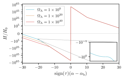
Figure 6: For case A, the dependence of the DE epoch with the parameter $\Omega_{\Lambda}$. Smaller values lead to earlier DE epochs. This behavior is also noticed in case B, but, since in case B the DE epoch happens in the expanding phase, smaller values of $\Omega_{\Lambda}$ will imply a later DE epoch. We included a zoom-in of the narrow interval around the DE phase, showing the constance of $H$ around it.

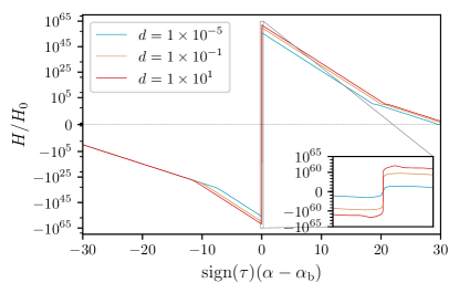
Figure 7: For case B, the dependence of the background dynamic with the parameter $d$. Smaller values of $d$ implies in longer matter duration. This behavior is also noticed in case A. We included a zoom-in of the narrow interval around the bounce, showing the behaviors of $H$ using different values of $d$.

The bounce happens in $\alpha=\alpha_{\mathrm{b}}$, and the two peaks are the highest values of $H$ reached by the system, further on referred as $H_{\mathrm{max}}$. The peaks happen when $\dot{H}=0$ and we can use them to define the duration of the bounce, $\delta_{\mathrm{b}}$. They can be better noticed in the zooms depicted in Figs. 7 and 8. The closer the peaks are in the plots, the smaller is $\delta_{\mathrm{b}}$ (faster bounce).

In what concerns the quantum solutions, the variation of the parameters $d$, $\sigma$ and $\alpha_{\mathrm{b}}$ directly changes the time and energy scales of the bounce. When increasing $d$, the frequency in Eqs. (27) and (28) is higher and it is possible that the background oscillates close to the bounce, Fig. 7.

Another important influence of $d$ is in the duration of the matter phase in contraction. Using Eq. (37), we can mark the onset of the matter-fluid phase by choosing a fixed $\epsilon_{\lambda}$ (for example $10^{-4}$). Then, it is clear from Eq. (43) that $a_{\lambda}$ (marking the beginning of the matter-fluid phase) is proportional to $|d|^{2/3}$. Hence, larger $d$ yields longer stiff-matter phases. This effect can be seen in Fig. 7. In the expanding era, which contains a DE phase, the same Eq. (37) can be used, but now $C_{2}=1/2$, and the connection to $d$ is through ${\bar{a}}_{0}$ given by Eq. (55). Consequently, $a_{\lambda}\propto|d|^{1/3}$. In the expanding era of Fig. 7 we can see that the DE plateau shifts by a smaller $\delta\alpha$ than the matter-fluid era shift in the contraction phase.

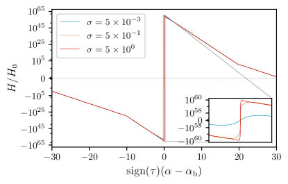
Figure 8: For case B, the dependence of the $H_{\mathrm{max}}$ with $\sigma$. $H_{\mathrm{max}}$ is an important parameter in order to determine the validity of the canonical quantization, since we should maintain the energy scale of the bounce below Planck scale.

The parameter $\sigma$ is relevant only in the quantum phase. Figure 8 shows that larger $\sigma$’s implies in higher energy and in shorter time scales in the bounce. This can be easily understood looking again to Eqs. (27) and (28). The hyperbolic functions have the argument $\sigma^{2}\alpha\phi$ [see for instance Eq. (29)] and they saturate when the argument is of the order of $11$ [$x\approx\coth(11)\approx 1+\mathcal{O}{\left(10^{-10}\right)}$]. Hence, a larger value for $\sigma$ leads to a faster saturation of the hyperbolic functions and, consequently, to an earlier stiff-fluid epoch. Furthermore, in the small $\alpha$ and $\phi$ approximation, the value of $|H_{\mathrm{max}}|$ is also proportional to $\sigma$, meaning that larger values of $\sigma$ generate more energetic bounces.

A similar argument leading to higher values of $|H_{\mathrm{max}}|$ can be used when analyzing the influence of $\alpha_{\mathrm{b}}$, Fig. (9). More profound bounces imply in a longer stiff-matter epoch, as we can see in the transitions of the slopes in Fig. (9). During that period $|H|$ has more time to increase leading to high-energy scale bounces.

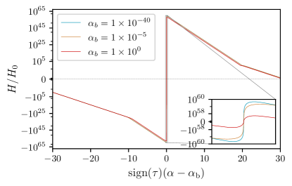
Figure 9: For case B, the dependency of the bounce energy scale with the minimum scale factor. Smaller values of $\alpha_{\mathrm{b}}$ allows a longer contraction that increases $|H_{\mathrm{max}}|$.

Finally, in Fig. (10) we observe that $\mathcal{X}_{\mathrm{b}}$, controlling the matching point between the classical and quantum branches, influences the duration of the dust domination era. This turns out to be crucial for the perturbations, not only because the power-spectrum slope depends on which fluid dominates when the mode leaves the Hubble radius, but also because the spectrum amplitude depends on how long the mode evolves in each fluid-like epoch.

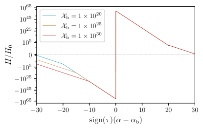
Figure 10: For case B, the duration of matter epoch is longer for bigger values of $\mathcal{X}_{\mathrm{b}}$.

VI Primordial perturbation

The perturbed Einstein’s equations can be recast in a very simple and objective manner combining the scalar perturbation in the metric and in the matter component by means of the gauge invariant curvature perturbation $\zeta$. The action that gives the dynamic for the perturbations comes from the first-order perturbed Einstein-Hilbert action and reads (Falciano et al., 2013, Eq. (66))

$$S=\int\mathrm{d}\tau\,\mathrm{d}x^{3}\frac{z^{2}}{2}\left({\zeta}^{\prime 2}+\frac{N^{2}\zeta\Delta\zeta}{a^{2}}\right),\;\;z^{2}\equiv\frac{3a^{3}x^{2}}{\kappa^{2}N},$$ (58)

where $\Delta$ is the spacial Laplacian, $\zeta$ is the gauge invariant dimensionless curvature perturbation, and the time operator is defined by $\prime\equiv\mathrm{d}/\mathrm{d}\tau$. The equation of motion for $\zeta$ is obtained by the variational principle, and after the field decomposition it reads

$$\zeta^{\prime\prime}_{k}+2\frac{z^{\prime}}{z}{\zeta_{k}^{\prime}}+\frac{N^{2}k^{2}}{R_{H}^{2}a^{2}}\zeta_{k}=0.$$ (59)

In the above equations, we used the dimensionless time $\tau$ [Eq. (39)],

$$N=\frac{\mathrm{d}t}{\mathrm{d}\tau}=\frac{\tau}{H}.$$

Here $k$ is measured in units of $R_{H}^{-1}$, $z$ and $\zeta_{k}$ have dimensions of $\mathrm{lenght}^{-3/2}$ and $\mathrm{lenght}^{3/2}$ respectively.

We are in the domain of linear perturbation theory, in which the scalar, vector and tensor perturbations decouple. The tensor perturbation $h_{ij}$, whose amplitude of any of its two polarizations will be refereed by $h$, presents a similar action, i.e.,

$$S=\int\mathrm{d}\tau\,\mathrm{d}x^{3}\frac{z_{h}^{2}}{2}\left(h^{\prime 2}+\frac{N^{2}h\Delta h}{a^{2}}\right),\;\;z_{h}^{2}\equiv\frac{a^{3}}{4\kappa^{2}N}.$$ (60)

Its equation of motion can be easily deduced from the action above,

$$h_{k}^{\prime\prime}+2\frac{z_{h}^{\prime}}{z_{h}}{h_{k}^{\prime}}+\frac{N^{2}k^{2}}{R_{H}^{2}a^{2}}h_{k}=0,$$ (61)

where $h_{k}$ also has dimension of $\mathrm{length}^{3/2}$. The above formulation can be found in the literature, for instance in Mukhanov et al. (1992); Peter and Uzan (2009); Brandenberger (2004). Here we introduced only the necessary information in order to define the observational probes that we will calculate. The quantities constrained by the observations are the power spectra,

$$\Delta_{\zeta_{k}} \equiv\frac{k^{3}|\zeta_{k}|^{2}}{R_{H}^{3}2\pi^{2}}=\frac{\ell_{{}_{\mathrm{P}}}^{2}}{R_{H}^{2}}\frac{4k^{3}|\tilde{\zeta}_{k}|^{2}}{3\pi},$$ (62)

$$\Delta_{h_{k}} \equiv\frac{k^{3}|h_{k}|^{2}}{R_{H}^{3}2\pi^{2}}=\frac{\ell_{{}_{\mathrm{P}}}^{2}}{R_{H}^{2}}\frac{16k^{3}|\tilde{h}_{k}|^{2}}{\pi},$$ (63)

where we introduced the dimensionless mode functions

$$\zeta_{k}\equiv\sqrt{\frac{\kappa^{2}R_{H}}{3}}\tilde{\zeta}_{k},\qquad h_{k}\equiv\sqrt{4\kappa^{2}R_{H}}\tilde{h}_{k}.$$ (64)

The spectral indexes for the scalar curvature perturbation $\zeta$ and tensor perturbation $h$ labeled by the subscripts s and T are, respectively,

$$n_{\mathrm{s,T}}-1\equiv\left.\frac{\mathrm{d}\log(\Delta_{\zeta_{k},h_{k}})}{\mathrm{d}\log k}\right|_{k=k_{*}}$$ (65)

and the tensor-to-scalar ratio

$$r\equiv 2\left.\frac{\Delta_{h_{k}}}{\Delta_{\zeta}}\right|_{k=k_{*}},$$ (66)

where the factor $2$ comes to account for the two polarizations of the tensor perturbation. We use the same pivotal scale as in Planck Collaboration et al. (2015b), $k_{*}=0.05R_{H}\;\mathrm{Mpc}^{-1}$. The latest Planck release estimates for long wave-lengths $\Delta_{\zeta_{k}}\approx 10^{-10}$, $n_{\mathrm{s}}\approx 0.96$ and $r<0.1$ Planck Collaboration et al. (2015b).

Following the results from Peter et al. (2007); Peter and Pinto-Neto (2008), the spectral index for the modes entering the horizon during the domination of a fluid with EoS $w$ is

$$n_{\mathrm{s}}=1+\frac{12w}{1+3w}.$$ (67)

In case B, the spectrum is scale invariant when entering the horizon while $w=0$, matter epoch. Depending on the duration of the matter contraction, some very small scale modes may enter during the transition to the stiff-matter phase, $w=1$, leading to a blue spectrum. For case A, besides the above two possibilities, there is also the influence of the transient DE epoch in large scale modes. Hence, although case A is more academic, it should be quite interesting to evaluate the exact spectral index in this case in order to estimate the impact of the presence a transient DE in the contracting phase of a matter bounce in the standard results.

VI.1 Initial vacuum perturbations

It is usually proposed in current cosmological models that the inhomogeneities in the Universe have their origin in primordial vacuum quantum fluctuations. In the inflationary scenario, the exponential growth of the scale factor are responsible for amplifying those quantum fluctuations. After a $60$ e-fold expansion they have enough amplitude to fit the CMB observations.

Bouncing models assume the same mechanism for the origin of inhomogeneities, but replaced in the far past of the contracting phase. Some scenarios may find difficulty in providing the Minkowsky vacuum as initial conditions. This is the case when the cosmological constant is considered Maier et al. (2011).

In the present case, the scalar field behaves like a matter fluid and the usual quantization of the adiabatic vacuum fluctuations in a Minkowsky space-time coincides with the WKB solution with positive energy for the Mukhanov-Sasaki variable $v\equiv z\zeta$. The equation of motion (59) can be written

$$v_{k}^{\prime\prime}+w_{k}^{2}v_{k}=0,$$ (68)

where,

$$w_{k}^{2}(\eta,k)\equiv\frac{N^{2}k^{2}}{a^{2}R_{H}^{2}}-\frac{z^{\prime\prime}}{z}.$$ (69)

Note that the expressions above reduce to the usual conformal time equations for $N=a$.

A solution of the above equation can be expressed in terms of the WKB approximation (see for example Peter and Uzan (2009)), which has a certain limit of validity. Let us define,

$$Q_{\mathrm{WKB}}=\frac{3}{4}\left(\frac{w_{k}^{\prime}}{w_{k}}\right)^{2}-\frac{1}{2}\frac{w_{k}^{\prime\prime}}{w_{k}}.$$ (70)

In the regime in which

$$\left|\frac{Q_{\mathrm{WKB}}}{w_{k}^{2}}\right|\ll 1,$$ (71)

the solution is

$$\tilde{v}_{k}^{\mathrm{WKB}}\approx\frac{1}{\sqrt{2w_{k}}}\mathrm{e}^{\pm i\int\mathrm{d}\tau w_{k}}.$$ (72)

The matter contraction satisfies (71) and Eq. (72) not only gives the initial conditions but also a good approximation for the solution of Eq. (68) while condition (71) is satisfied.

For $N^{2}k^{2}/(a^{2}R_{H}^{2})\gg|z^{\prime\prime}/z|$ the initial vacuum conditions are reduced to

$$v_{\mathrm{ini}} =\frac{1}{\sqrt{2k}}\sqrt{\frac{aR_{H}}{N}},$$ (73)

$$\left.\frac{\mathrm{d}{}v}{\mathrm{d}\tau}\right|_{\mathrm{ini}} =i\sqrt{2k}\sqrt{\frac{N}{aR_{H}}},$$ (74)

where we have set the initial phase factor equal to zero. Again, we can recover the usual vacuum conditions choosing the conformal time lapse function $N=a$. The tensor modes $h$ can be expressed in terms of the variable

$$\mu=z_{h}h,$$ (75)

which satisfies similar equations as $v$, but with $z_{h}$. The same treatment given to the quantization of $v$ can be performed for $\mu$ and the initial conditions are equivalent for the tensor modes.

In the adiabatic limit, the perturbations are in a high oscillatory regime and the numerical calculations become contrived. A very common approach to numerically solve the perturbations is to consider the WKB solution until $N^{2}k^{2}/(a^{2}R_{H}^{2})>|z^{\prime\prime}/z|$ and to switch to the numerical calculation just before the saturation of the inequality. The problem with this approach is that, by construction, the WKB approximation is worse and worse as we approximate the saturation point. Thus, we must balance two problems, first if we start the numerical evolution very close to the saturation we would need a high order WKB approximation to get a reasonable initial condition. The high order WKB approximation needs high order time derivatives of the background functions, which in turn is badly defined numerically or involves complicated background functions also numerically error prone. If we decide to start away from the saturation point we need to deal with the highly oscillatory period, in which the processing time is longer and the numerical errors accumulate with the oscillations. To circumvent the above mentioned problems, we will use the action angle variables to rewrite the perturbations dynamics and numerically solve the new sets of equations. These variables are better suited to the high oscillatory regime and allows us to use initial conditions away from the saturation point.

VI.2 Action angle variables

The Action Angle (AA) variables can be used to solve high oscillatory differential equations Vitenti (2015); Peter et al. (2016); Celani et al. (2017). General linear oscillatory systems have a quadratic Hamiltonian in the form

$$\mathcal{H}=\frac{\Pi_{\tilde{\zeta}_{k}}^{2}}{2m}+\frac{m\nu^{2}}{2}\tilde{\zeta}_{k}^{2},$$ (76)

where $m$ is the associated “mass” of the system and $\nu$ the frequency. The generalized variable and associated momenta are $\tilde{\zeta}_{k}$ and $\Pi_{\tilde{\zeta}_{k}}$, respectively.

From action (58) and the definition of the dimensionless variables (64), we can easily deduce that

$$m=\frac{\kappa^{2}R_{H}z^{2}}{3}=\frac{a^{3}x^{2}R_{H}}{N},\qquad\nu=\frac{Nk}{aR_{H}}.$$ (77)

The Hamilton equations are

$$\zeta^{\prime}_{k}=\frac{\Pi_{\zeta_{k}}}{m},\qquad\Pi^{\prime}=-m\nu^{2}\zeta_{k}.$$ (78)

AA variables are based on the adiabatic invariant of oscillatory systems Landau and Lifshitz (1976). A real solution for the Hamilton equations above can be rewritten in terms of the variables $(I,\;\theta)$, implicit defined by

$$\tilde{\zeta}^{\mathrm{a}}_{k} =\sqrt{\frac{2I}{m\nu}}\sin\left(\theta\right),$$ (79)

$$\Pi^{\mathrm{a}}_{\tilde{\zeta}_{k}} =\sqrt{2Im\nu}\cos\left(\theta\right).$$ (80)

Deriving the above expressions and using the Hamilton equations, we find the equation of motion in terms of the new variables $\theta$ and $I$ are, respectively,

$$I^{\prime} =-I\frac{(m\nu)^{\prime}}{m\nu}\cos\left(2\theta\right),$$ (81)

$$\theta^{\prime} =\nu+\frac{1}{2}\frac{(m\nu)^{\prime}}{m\nu}\sin\left(2\theta\right).$$ (82)

The second real solution $\zeta^{\mathrm{b}}$ introduces another pair of AA variables, $(J,\;\psi)$, again implicit defined by

$$\tilde{\zeta}^{\mathrm{b}}_{k} =\sqrt{\frac{2J}{m\nu}}\sin\left(\psi\right),$$ (83)

$$\Pi_{\tilde{\zeta}_{k}}^{\mathrm{b}} =\sqrt{2Jm\nu}\cos\left(\psi\right).$$ (84)

They follow the same equations of motion

$$J^{\prime} =-J\frac{(m\nu)^{\prime}}{m\nu}\cos\left(2\psi\right),$$ (85)

$$\psi^{\prime} =\nu+\frac{1}{2}\frac{(m\nu)^{\prime}}{m\nu}\sin\left(2\psi\right).$$ (86)

The final complex solution is defined by

$$\tilde{\zeta}_{k}=\frac{\tilde{\zeta}_{k}^{\mathrm{a}}+i\tilde{\zeta}_{k}^{\mathrm{b}}}{2i},$$

with the real and imaginary parts satisfying the normalization condition imposed by the initial quantum vacuum perturbations, i.e.,

$$\sqrt{IJ}\sin\left(\psi-\theta\right)=1$$ (87)

We will define the variables $\epsilon$, $\bar{\theta}$ and $\Delta\theta$ in order to re-write the above equations so the constraint will be automatically satisfied all along the evolution. Defining

$$\sinh\left(\epsilon\right) =\cot\left(\Delta\theta\right),$$ (88)

$$\Delta\theta =\psi-\theta,$$ (89)

$$\bar{\theta} =\frac{\psi+\theta}{2},$$ (90)

we can easily demonstrate the relations

$$\sqrt{IJ} =\cosh\left(\epsilon\right),$$ (91)

$$\sin\left(\Delta\theta\right) =\frac{1}{\cosh\left(\epsilon\right)},$$ (92)

$$\cos\left(\Delta\theta\right) =\tanh\left(\epsilon\right).$$ (93)

Differentiating Eqs. (90) and (91) and using Eqs. (92) and (93) to rewrite $\psi$ and $\theta$ in terms of $\epsilon$ and $\bar{\theta}$ we find

$$\bar{\theta}^{\prime} =\nu+\frac{(m\nu)^{\prime}}{m\nu}\tanh\left(\epsilon\right)\sin\left(\bar{\theta}\right)\cos\left(\bar{\theta}\right),$$ (94)

$$\epsilon^{\prime} =-\frac{(m\nu)^{\prime}}{m\nu}\cos\left(2\bar{\theta}\right).$$ (95)

The system is not yet fully described, since we have only the dynamics for a composition of $I$ and $J$ through $\epsilon$. Introducing $\gamma$ by the relation

$$\mathrm{e}^{\gamma}=\sqrt{\frac{I}{J}},$$ (96)

we easily obtain

$$\gamma^{\prime}=-2\frac{(m\nu)^{\prime}}{m\nu}\frac{\sin\left(\bar{\theta}\right)\cos\left(\bar{\theta}\right)}{\cosh\left(\epsilon\right)},$$ (97)

and $I$ and $J$ can be recovered using

$$I =\mathrm{e}^{\gamma}\cosh(\epsilon),$$ (98)

$$J =\mathrm{e}^{-\gamma}\cosh(\epsilon).$$ (99)

Finally the complete set of equations that replaces Eqs. (81), (82), (85), (86) already accounting the constraint (87) is

$$\bar{\theta}^{\prime} =\nu+\frac{(m\nu)^{\prime}}{m\nu}\tanh\left(\epsilon\right)\sin\left(\bar{\theta}\right)\cos\left(\bar{\theta}\right),$$ (100)

$$\epsilon^{\prime} =-\frac{(m\nu)^{\prime}}{m\nu}\cos\left(2\bar{\theta}\right),$$ (101)

$$\gamma^{\prime} =-2\frac{(m\nu)^{\prime}}{m\nu}\frac{\sin\left(\bar{\theta}\right)\cos\left(\bar{\theta}\right)}{\cosh\left(\epsilon\right)}.$$ (102)

Using these new variables, the two real linearly independent solutions can be recast as

$$\tilde{\zeta}_{k}^{a} =\frac{\mathrm{e}^{\gamma/2}}{\sqrt{m\nu}}\left[\mathrm{e}^{\epsilon/2}\sin\left(\bar{\theta}\right)-\mathrm{e}^{-\epsilon/2}\cos\left(\bar{\theta}\right)\right],$$ (103)

$$\tilde{\zeta}_{k}^{b} =\frac{\mathrm{e}^{-\gamma/2}}{\sqrt{m\nu}}\left[\mathrm{e}^{\epsilon/2}\sin\left(\bar{\theta}\right)+\mathrm{e}^{-\epsilon/2}\cos\left(\bar{\theta}\right)\right].$$ (104)

Now we have to rewrite the adiabatic vacuum initial conditions, for that purpose we use the adiabatic limit ${(m\nu)^{\prime}}/{m\nu}\rightarrow 0$. Expanding in the leading order in ${(m\nu)^{\prime}}/{m\nu}$ the set of equations provides

$$\epsilon \approx\epsilon_{0},$$ (105)

$$\gamma \approx\gamma_{0},$$ (106)

$$\bar{\theta} \approx\bar{\theta}_{0}+k\eta.$$ (107)

Using the above approximations to calculate the complex $\tilde{\zeta}_{k}$, we have, as an initial condition, that the following choice recovers the leading order WKB approximation, Eqs. (73) and (74):

$$\epsilon_{0}=\gamma_{0}=0,$$ (108)

which, naturally, satisfies the Eq. (87). The real solutions using this choice are

$$\tilde{\zeta}_{k}^{a} =\sqrt{\frac{2}{m\nu}}\sin\left(\bar{\theta}-\frac{\pi}{4}\right),$$

$$\tilde{\zeta}_{k}^{b} =\sqrt{\frac{2}{m\nu}}\cos\left(\bar{\theta}-\frac{\pi}{4}\right),$$

then, consequently, the complex solution is

$$\tilde{\zeta}_{k}=\frac{\mathrm{e}^{-i\left(\bar{\theta}-{\pi}/{4}\right)}}{\sqrt{2m\nu}}.$$

Because it is just a phase, we can choose $\bar{\theta}_{0}=\pi/4$.

The same treatment follows through in the case of the dimensionless tensor perturbation, with the only difference being the “mass” definition

$$m_{h}=4\kappa^{2}R_{H}z_{h}^{2}=\frac{a^{3}R_{H}}{N},\qquad\nu_{h}=\frac{Nk}{aR_{H}}.$$ (109)

A general purpose integrator for systems described by an action in the form (76) was implemented as part of the NumCosmo (numerical cosmology library) Vitenti and Penna-Lima (2014). The abstract implementation of the harmonic oscillator action angle is provided by the object NcmHOAA Vitenti (2017). The adiabatic and tensor mode objects, respectively NcHIPertAdiab and NcHIPertGW, are built on top of NcmHOAA, connecting it to the exponential potential background model NcHICosmoVexp. We should stress that these codes can be used to any background model, all one needs to do is to implement the interface which calculates the mass $m$ and frequency $\nu$ of the model.

	$d$	$\sigma$	$\alpha_{\mathrm{b}}$	$\mathcal{X}_{\mathrm{b}}$
set1	$-9\times 10^{-4}$	$9$	$8.3163\times 10^{-2}$	$2\times 10^{36}$
set2	$-9\times 10^{-4}$	$100$	$7.4847\times 10^{-3}$	$4\times 10^{36}$
set3	$-0.1$	$4$	$10^{-5}$	$6\times 10^{37}$
set4	$-0.1$	$4$	$10^{-7}$	$6\times 10^{37}$

Table 3: Model parameters for four different cases in which the present model produces $\Delta_{\zeta}$ close to $10^{-10}$, and scale invariant spectra. The relevant background quantities are presented in Fig. (11) through (14), while the modes evolution can be seen in Fig. (15). The DE scale is fixed at $\Omega_{\Lambda}=1$.

VII Numerical solutions for the perturbations

Using the AA variables, we can calculate the power spectra for both scalar and tensor perturbations. In this section, we will present these solutions, and discuss how the basic parameters of the model influence the primordial perturbations. We will focus in case B, which is a complete background that addresses the problem of DE in bounce models by means of a single scalar field, in this analysis we keep fixed both $\Omega_{\Lambda}=1$ and $\Omega_{d}=1$. Here we analyze in detail four parameter sets defined in Tab. 3.

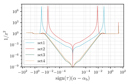
Figure 11: Evolution of the $1/x^{2}$ term given four sets of parameters, set1, set2, set3 and set4, appearing in Tab. 3. The distance between peaks is controlled by the $\sigma$ parameter, while its height is determined by how much the background bouncing trajectory gets close to the cyclic solutions presented in Fig. (5), which in turn is defined by the value of $\alpha_{\mathrm{b}}$.

Before moving to the solutions themselves, it is worth to take a look at the differences between the scalar mode and the tensor mode evolution. The super Hubble solutions for Eqs. (76) are, at leading order,

$$\tilde{\zeta}_{k} =A^{1}_{k}\left[1+\mathcal{O}\left(\nu^{2}\right)\right]+A^{2}_{k}\left[\int\frac{\mathrm{d}\tau}{m}+\mathcal{O}\left(\nu^{2}\right)\right],$$ (110)

$$\tilde{h}_{k} =B^{1}_{k}\left[1+\mathcal{O}\left(\nu_{h}^{2}\right)\right]+B^{2}_{k}\left[\int\frac{\mathrm{d}\tau}{m_{h}}+\mathcal{O}\left(\nu_{h}^{2}\right)\right],$$ (111)

where changing the integration limits in the integrals above result in a redefinition of $A^{1}_{k}$ and $B^{1}_{k}$. Using the expression for the masses in Eqs. (77) and (109), we recast the integral as

$$\int\frac{\mathrm{d}\tau}{m} =\frac{1}{R_{H}}\int\mathrm{d}\tau\frac{N}{x^{2}a^{3}}=\frac{1}{R_{H}}\int\frac{\mathrm{d}{}t}{x^{2}a^{3}},$$ (112)

$$\int\frac{\mathrm{d}\tau}{m_{h}} =\frac{1}{R_{H}}\int\mathrm{d}\tau\frac{N}{a^{3}}=\frac{1}{R_{H}}\int\frac{\mathrm{d}{}t}{a^{3}}.$$ (113)

In the classical contracting branch of case B, $x$ varies between $(1/\sqrt{2},\;1)$, while the scale factor goes through a large contraction. In other words, the value of this integral will be dominated by the values of $a$ near the bounce phase, where $a$ attains its smallest value (see Vitenti and Pinto-Neto (2012) for a detailed analysis of this integral). Nonetheless, when the quantum phase begins, the value of $x$ is no longer restricted to $(1/\sqrt{2},\;1)$. For example, in Fig. 11, we show three time evolutions for $1/x^{2}$ using four different sets of parameters.

During the matter phase $1/x^{2}\approx 2$, and during the stiff matter domination, $1/x^{2}\approx 1$. Therefore, in the classical phase, the presence of $1/x^{2}$ in the integral (110) increases its value by a maximum factor of two. On the other hand, throughout the quantum phase, different parameter sets result in quite different behaviors, as can be seen in Fig. 11. The set1 curve shows that the presence of $1/x^{2}$ in the aforementioned integral will result in a sharp increase in the spectrum amplitude around $|\alpha-\alpha_{\mathrm{b}}|\approx 10^{-1}$. This effect takes place slightly closer to the bounce in set2. Furthermore, in set3 we show a solution where the peaks are negligible, and hence there is no further increase of the perturbation amplitudes around the bounce. The phase space plot in Fig. 12 elucidates what is happening. The set1 and set2 configurations are such that the system passes closes to the cyclic solutions (see Fig. 5), and the curve is near vertical, $\alpha$ changes abruptly with $\phi$, making $x$ close to zero during this interval. The scalar field shortly behaves as a DE fluid, implying a momentarily large deceleration (acceleration), which enhance the scalar perturbations. We also added the set3 and set4 to show solutions which pass far from these cyclic solutions. In this case, the evolution of $\alpha$ with respect to $\phi$ is smoother, resulting in bigger values of $x$.

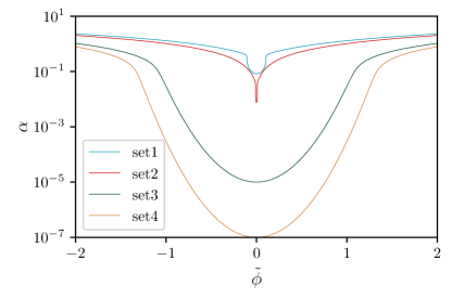
Figure 12: Phase space evolution for the four sets of parameters appearing in Tab. 3. Note that the set1 and set2 curves are almost vertical near the bounce. This happens because they pass close to the periodic trajectories (see Fig. 5 for a full picture of the phase space trajectories). At these points, $x\propto\mathrm{d}\phi/\mathrm{d}\alpha\approx 0$, which results in the peaks seen in Fig. 11. Contrastingly, the set3 and set4 curves pass far from the center points of Fig. 5, resulting in a smoother transition through the bounce phase. With all parameters fixed, we can control how close one gets to the cyclic solutions by increasing the value of $\alpha_{\mathrm{b}}$. One can also see in the figure, by comparing set1 with set2, that a larger $\sigma$ induces a faster bounce.

On the other hand, the tensor mode amplitudes do not depend on $x$, see Eq. (113). In Fig. 13, we present the evolution of both integrands of Eqs. (112) and (113). Note that the first peak to the left in both figures is just the usual increase in amplitude related to the contraction, while during the bounce itself we have two different behaviors depicted. The tensor modes, which depend only on the lapse function $N$ and the scale factor, are sensitive to the peaks of $N$ at the bounce, whereas for scalar modes, the presence of the $1/x^{2}$ term in the integrand overcomes the $N$ dependence around the bounce. Here we would like to emphasize that the exact dynamics controlling the bounce is extremely important to determine the amplitude of the spectrum. Integrating only the classical phase, the first left peak in both integrands would provide similar amplitudes for both scalar and tensor modes, implying in a larger than one tensor-to-scalar ratio (see, for example, Ref. Quintin et al. (2015)). However, one cannot stop at the classical phase, since the bounce evolution will left a definite imprint on the amplitudes: an increase in the tensor mode amplitude at the bounce, and two amplifications of the scalar modes at two symmetric points around the bounce. Hence, any new physics around the bounce producing this kind of effect can be physically relevant, and its consequences must be evaluated with care.

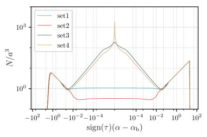
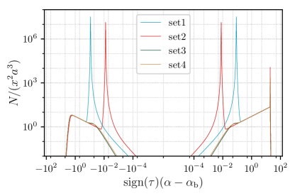
Figure 13: Integrand of the super Hubble approximation for the tensor modes (left panel) and scalar modes (right panel). It is worth noting that the presence of the $1/x^{2}$ term in the scalar mode integrals, which goes through zero during the bounce phase, overcomes any possible additional contribution to the amplitude from the peak in the lapse function $N=\tau/H$. Nevertheless, the tensor modes are sensitive to the peaks in $N$.

The contracting phase with a matter era puts this model in the category of the matter bounce scenarios. Previous works on the field obtained the bounce by means of a second scalar field with a ghost-type Lagrangian. Choosing wisely the parameters of the ghost scalar field, the bounce takes place only very close to the singularity, and the perturbations are studied, sometimes, without taking it into account. The results obtained in the literature about matter bounces can be summarized as follows: the spectrum is scale invariant; the tensor-to-scalar ratio is usually larger then measured in CMB if the scalar field is canonical and the bounce is symmetric; attempts to solve this problem assuming the validity of GR all along results in the increase of non-Gaussianities, which seems to suggest a no-go theorem for bounce cosmologies Quintin et al. (2015); Li et al. (2017). Our results point to a new direction: bounces which are out of the scope of GR can lead to new ways to decrease $r$, and they should be investigated with care. In our model, the decrease of the tensor-to-scalar ratio relies on the actual bounce dynamics in a non-trivial way, due to quantum effects. The increase in amplitude of the scalar and tensor modes take place at different times and are controlled by distinct parameters. The consequences of that for non-Gaussianities is something yet to be investigated.

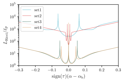
Figure 14: Time evolution of the Ricci scale for all sets appearing in Tab. 3. The parameter $d$ controls how close the scale gets to the Planck length and set3 and set4 are in the limit of validity of our model. Thus, a large (in module) value of $d$ would violate this constraint. Note also that faster bounces (for instance, set2) result in stronger oscillations of $L_{R}$ near the bounce. This means that faster bounces must take place at even higher scales in order to avoid a violation of $L_{R}/\ell_{{}_{\mathrm{P}}}>1$ during the oscillations.

Concerning the amplitude growth in the classical regime, a known result is that they grow more substantially during a matter epoch then during the stiff matter one. This can be seen by looking at the super Hubble approximations in Eqs. (112) and (113). During the matter domination, $N/a^{3}\approx\tau/a^{3/2}$, while for stiff matter $N/a^{3}\approx\tau$, where we are using that $N=\tau/H$, and $H\propto a^{-3/2}$ in the matter phase and $H\propto a^{-3}$ at the stiff phase. Since this part of the amplitude growth is determined by the matter epoch duration, it is closely connected with the parameters $d$ and $\mathcal{X}_{\mathrm{b}}$, which also control the bounce depth.

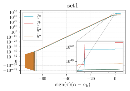
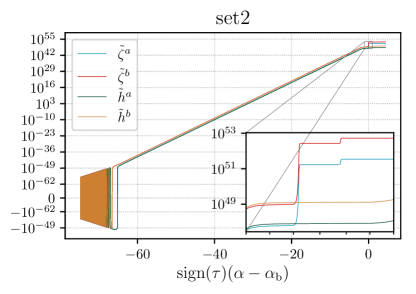
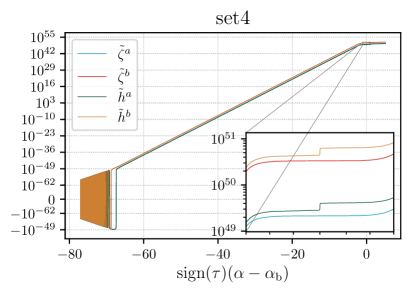
Figure 15: Evolution of the mode functions $\tilde{\zeta}_{k}$ and $\tilde{h}_{k}$ for set1, set2, set3 and set4. In the detail, we can see the result of the integration of the two peaks in Fig. 11 for the scalar mode in the upper panels and the single peak of Fig. 13 integration for the tensor mode in the lower panels. For example, in the upper left figure, the first peak around $-0.1$ increases the amplitude of $\tilde{\zeta}^{a}$ and the second peak at $+0.1$ double this value. In contrast, since the tensor perturbations amplitude does not depend directly on the evolution of $x$, they are not modified by these peaks. Nonetheless, the tensor amplitude is sensible to peaks in the lapse function $N$. Hence, for set3 and set4 where these peaks are pronounced, we have an increase in the amplitude of tensor perturbations at the bounce, which is otherwise overcome by scalar perturbations in the cases where the $1/x^{2}$ term become relevant.

We emphasize that the parameter choices are implicit determinations of the background model initial conditions (including the wave function parameters), as already mentioned. The results for the power spectra at the pivotal mode $k_{*}$ are:

$$\mathrm{set1:} \left.\Delta_{\zeta_{k}}\right|_{k=k_{*}}=1.4\times 10^{-10},\; r=1.9\times 10^{-7},$$

$$\mathrm{set2:} \left.\Delta_{\zeta_{k}}\right|_{k=k_{*}}=4.6\times 10^{-11},\; r=1.3\times 10^{-5},$$

$$\mathrm{set3:} \left.\Delta_{\zeta_{k}}\right|_{k=k_{*}}=1.2\times 10^{-14},\; r=56,$$

$$\mathrm{set4:} \left.\Delta_{\zeta_{k}}\right|_{k=k_{*}}=1.7\times 10^{-14},\; r=59.$$

The time evolution for this same pivotal mode is shown in Fig. 15. Observe that, for set1 and set2, the extra enhancement of the scalar amplitude due to the quantum effects takes it to a value close to the observed one $\left.\Delta_{\zeta_{k}}\right|_{k=k_{*}}\approx 10^{-10}$. On the contrary, the power spectra obtained from set3 and set4 have an amplitude smaller than the required by observations, even though their bounces are deeper ($\mathcal{X}_{\mathrm{b}}\approx 10^{36}$ for set1 and set2 and $\mathcal{X}_{\mathrm{b}}\approx 10^{37}$ for set3 and set4). In principle, one could choose the parameters in order to make the bounce deeper, hoping to get the right amplitude. Nevertheless, we must take care to not go beyond the scale of validity of these models. One should verify whether the energy scale of the bounce is not dangerously close to the Planck energy scale, where our simple approach would not be appropriate. The curvature scale at the bounce is given by the Ricci scalar,

$$R=12H^{2}+6\dot{H},\quad L_{R}=1/\sqrt{R},$$ (114)

and Ricci scale $L_{R}$ should not be smaller than the Planck length. Figure 14 displays the Ricci scale evolution for all parameter sets. This figure shows that the absolute value of $d$ controls the minimum scale $L_{R}$ attained around the bounce. This means that we could not increase the amplitudes of set3 and set4 by increasing $|d|$ without violating the validity of our approach.

In what concerns the spectral index, our modes of interest cross the potential during the matter domination phase. As such, their spectrum are very close to scale invariant. Again, this can be changed using a slight negative value for the matter phase EoS.

VIII Conclusion

We have studied the evolution of cosmological perturbations of quantum mechanical origin in a nonsingular cosmological model containing a single scalar field with exponential potential. The bounce is driven by quantum corrections of gravity in high-energy scales, but still smaller than the Planck energy scale, in which the canonical quantization of gravity may be applied.

In Secs. II, III and IV we presented two possibilities for the homogeneous and isotropic background dynamics: case A, which contains a DE epoch only in the contracting phase, and case B, in which the DE epoch happens only in the expanding phase. In both cases, the scalar field behaves like a dust fluid in the asymptotic past and future. The free parameters at our disposal were mapped to quantities with physical significance, as the duration of the matter contraction, the energy scales of the DE epoch and of the bounce phase, and their selection was equivalent to choose initial conditions for the numerical integration, hence allowing a better physical control of the whole scenario.

We restricted our attention mainly to case B, which is a matter bounce model with a DE epoch in the expanding phase, offering a complete background solution in which the DE epoch arises naturally in the expanding phase by means of the same scalar field that drives the bounce and the matter contraction. This is a bouncing model with DE where its presence does not cause any trouble in defining adiabatic vacuum initial conditions in the far past of the contracting phase (as described in Ref. Maier et al. (2011)), because it is dominated by dust. We numerically calculated the evolution of cosmological perturbations of quantum mechanical origin in such backgrounds. Scalar and tensor perturbations result to be almost scale invariant, and the parameters of the background can be adjusted to yield the good amplitudes for scalar and tensor perturbations, producing $r<0.1$. We have also seen that it was in the quantum bounce that the scalar perturbations were amplified with respect to tensor perturbations. Hence, the same quantum effects which produces the background bounce do also induce the property $r<0.1$. Our result shows that when GR is violated around the bounce, the influence of this phase on the evolution of cosmological perturbations can be nontrivial, and must be evaluated with care. Since we have only one scalar field, the perturbations were solved numerically for the whole background history, without approximations and matching conditions. Using the AA variables, we were able to construct a robust code where the details of the bounce effects on the perturbations could be appreciated for different background features. We have also found that longer the dust contraction, bigger are the amplitudes, a fact that was not noticed in other investigations.

We have thus obtained a bouncing model with a single canonical scalar field which produces the observed features of cosmological perturbations at linear order. Usually, canonical scalar fields in the framework of GR produces $r\geq 1$ for symmetric bounces  Allen and Wands (2004); Battarra et al. (2014). We should emphasize that, in our model, we get $r<1$ not because it is asymmetric, but because of violations of GR around the bounce due to quantum effects. The next step should be to evaluate non-Gaussianities in this model. Note that, as long as GR is not satisfied around the bounce, arguments based on the full validity of GR even at the bounce suggesting that non-Gaussianities should be huge in single scalar field bouncing models do not apply Quintin et al. (2015); Li et al. (2017). The evaluation of the non-Gaussianities must be made with care through the quantum bounce, as long as GR is not valid there. A consistent framework must be developed in order to perform this calculation correctly. This is one of our future investigations.

Note that this is a very simple model, with a single scalar field, but it is astonishing that it can produce alone the right amount of cosmological perturbations, and also yield a future DE phase. Hence, it is quite reasonable to pursue this route and try to complete the model in order to obtain more accurate scenarios for the real Universe. One possibility is to perform the same calculations when other fluids are present, as the classical extension of this model presented in Ref. Copeland et al. (1998). This is a much more involved calculation, where entropy perturbations must be considered.

In a future work, we will also study more deeply case A, which is a very interesting theoretical laboratory to investigate more precisely the influence of DE in a contracting phase. In that scenario, the cosmological perturbations evolve in a situation where usual adiabatic vacuum initial conditions can be posed normally, since DE behavior is transient and the background is matter dominated in the far past.

Finally, let us emphasize that the present model can accommodate non negligible primordial gravitational waves which might be detected in the near future. Hence, these models are observationally testable.