Investigating Galactic supernova remnant candidates using LOFAR

Abstract

We investigate six supernova remnant (SNR) candidates – $\mathrm{G}51.21+0.11$, $\mathrm{G}52.37-0.70$, $\mathrm{G}53.07+0.49$, $\mathrm{G}53.41+0.03$, $\mathrm{G}53.84-0.75$, and the possible shell around $\mathrm{G}54.1+0.3$ – in the Galactic Plane using newly acquired LOw-Frequency ARray (LOFAR) High-Band Antenna (HBA) observations, as well as archival Westerbork Synthesis Radio Telescope (WSRT) and Very Large Array Galactic Plane Survey (VGPS) mosaics. We find that $\mathrm{G}52.37-0.70$, $\mathrm{G}53.84-0.75$, and the possible shell around pulsar wind nebula $\mathrm{G}54.1+0.3$ are unlikely to be SNRs, while $\mathrm{G}53.07+0.49$ remains a candidate SNR. $\mathrm{G}51.21+0.11$ has a spectral index of $\alpha=-0.7\pm 0.21$, but lacks X-ray observations and as such requires further investigation to confirm its nature. We confirm one candidate, $\mathrm{G}53.41+0.03$, as a new SNR because it has a shell-like morphology, a radio spectral index of $\alpha=-0.6\pm 0.2$ and it has the X-ray spectral characteristics of a $1000-8000$ year old SNR. The X-ray analysis was performed using archival XMM-Newton observations, which show that $\mathrm{G}53.41+0.03$ has strong emission lines and is best characterized by a non-equilibrium ionization model, consistent with an SNR interpretation. Deep Arecibo radio telescope searches for a pulsar associated with $\mathrm{G}53.41+0.03$ resulted in no detection, but place stringent upper limits on the flux density of such a source if it is beamed towards Earth.

1 Introduction

There are many shell- and bubble-like objects in our Galaxy. For example, there are 295 supernova remnants (SNRs) in Green’s SNR catalog (just under half of which have only been detected in the radio; Green, 2014, 2017), 76 SNR candidates in a recent THOR+VGPS analysis (Anderson, et al., 2017), and $\sim 1500$ known HII regions (as well as $\sim 2500$ probable and $\sim 4000$ candidate HII regions) in the WISE HII region catalog (Anderson et al., 2014). This means that observations and surveys of the Galactic Plane capable of investigating shell-like objects, particularly observations differentiating between candidate HII regions and SNRs, are extremely useful. As there are many sources and candidates, targeting individual objects with a single pointing per object is impractical. Interferometers that can observe large areas of the sky at low-frequencies with wide frequency bandwidth should prove to be excellent tools for Galactic Plane investigations.

About 90% of SNRs and SNR candidates have been found in radio surveys (Anderson, et al., 2017), but it is thought that there could be many missing SNRs (e.g. Li et al., 1991; Tammann et al., 1994; Gerbrandt et al., 2014). Obtaining a more complete record of the SNR population, including confirming or rejecting the nature of SNR candidates, is important as it leads to better estimates of the Galactic supernova rate, the maximum ages of SNRs, and because SNRs are obvious locations for searching for young pulsars.

Low-frequency ($\lesssim 350\,\mathrm{MHz}$) Galactic Plane observations are useful for investigating SNRs and SNR candidates, particularly for differentiating between SNR candidates and HII regions, due to the typically steeper radio spectral indices of SNRs ($\alpha\approx-0.5$; Onić, 2013) as compared to HII regions ($\alpha\gtrsim 0$); where $S_{\nu}\,\propto\,\nu^{\alpha}$ for $S_{\nu}$ integrated flux density in $\mathrm{Jy}$ and $\nu$ frequency in $\mathrm{Hz}$ (Onić, 2013). This means that SNRs are brighter at lower frequencies, while HII regions are brighter at higher frequencies. However, there have been relatively few low-frequency surveys of the Galactic Plane with high angular resolution and sensitivity. A good illustration of the capability of such surveys for SNR searches was demonstrated by a $333\,\mathrm{MHz}$ survey with the Very Large Array (VLA) of the Galactic Center region (Brogan et al., 2006). This survey resulted in the discovery of 35 new candidate SNRs, 31 of which are now confirmed. Multi-wavelength analysis is required to confirm (or reject) SNR candidates, such as X-ray observations or further radio observations at a different frequency to confirm the spectral index.

The LOw-Frequency ARray (LOFAR; van Haarlem et al., 2013) is an interferometer that observes at low-frequencies with a large field-of-view (FoV; e.g. $\sim 11\,\mathrm{deg^{2}}$ using HBA Dual Inner mode), which means that it is ideal for observing and discovering steep-spectra objects and for differentiating between SNR candidates and HII regions. LOFAR consists of two arrays: the Low Band Antennas (LBA) and the High Band Antennas (HBA). The LBA observes between $10$ and $80\,\mathrm{MHz}$ while the HBA observes between $110$ and $250\,\mathrm{MHz}$. The wide FoV also introduces many technical difficulties regarding calibration and imaging, particularly as the ionosphere can introduce significant phase and amplitude variations across the FoV.

Here we discuss six SNR candidates in the FoV of proprietary LOFAR HBA observations (PI: J. D. Gelfand) that overlap with an archival Westerbork Synthesis Radio Telescope (WSRT) mosaic (Taylor et al., 1996) and an archival VLA Galactic Plane Survey (VGPS) mosaic (Stil et al., 2006). These SNR candidates were identified in a study of THOR+VGPS observations by Anderson, et al. (2017) and are: $\mathrm{G}51.21+0.11$, $\mathrm{G}52.37-0.70$, $\mathrm{G}53.07+0.49$, $\mathrm{G}53.41+0.03$, $\mathrm{G}53.84-0.75$, and $\mathrm{G}54.1+0.3$. In particular, we present a multi-frequency analysis of SNR candidate $\mathrm{G}53.41+0.03$. In Section 2 we present the observations. In Section 3 we present our results and in Section 4 we discuss the SNR candidates. We conclude in Section 5.

2 Observations and Analysis

2.1 Radio observations

We use radio observations at three different frequencies – $144\,\mathrm{MHz}$ (LOFAR HBA), $327\,\mathrm{MHz}$ (WSRT), and $1400\,\mathrm{MHz}$ (VGPS) – to investigate part of the Galactic Plane. Figure 1 shows the FoV where our LOFAR HBA observations overlap archival WSRT and VGPS mosaics.

We initially obtained and analyzed the LOFAR observations to investigate pulsar wind nebula (PWN) $\mathrm{G}54.1+0.3$ but, due to the large FoV, we also investigated other promising SNR candidates. The LOFAR observations are centered on the PWN. The observations were taken on 2015 June 12 as part of project LC4_011 (ObsID: 345918) and were performed in HBA Dual Inner mode (van Haarlem et al., 2013). This means that the inner 24 tiles of the remote stations were used resulting in a full-width half-maximum (FWHM) of the primary beam of $3.8^{\circ}$ and FoV of $\sim 11\,\mathrm{deg^{2}}$ in this configuration. The LOFAR HBA target and calibrator scans cover the frequency range from $118.7\,\mathrm{MHz}$ to $169.5\,\mathrm{MHz}$. The observing bandwidth was split into 260 subbands (SBs) with bandwidth of $195.3\,\mathrm{kHz}$ each. For these observations an 18 min calibrator scan of 3C380 was taken before and after the 3 hr target scan.

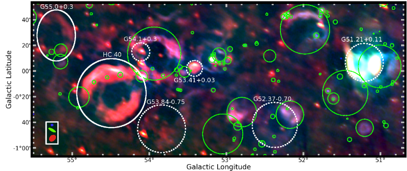
Figure 1: Observations of the Galactic Plane at $1.4\,\mathrm{GHz}$ (blue, VLA), $327\,\mathrm{MHz}$ (green, WSRT), and $144\,\mathrm{MHz}$ (red, LOFAR HBA). The synthesized beam sizes are shown in the bottom left corner. Known SNRs from Green’s SNR catalog (Green, 2014) are circled in solid white and candidate SNRs from Anderson, et al. (2017) are circled in dashed white. The green circles are HII regions from the WISE catalog (Anderson et al., 2014).

The LOFAR observations were flagged, demixed, and averaged as part of standard LOFAR pre-processing. Demixing involves removing the effects of the very bright radio sources, Cassiopeia A and Cygnus A, that affect LOFAR images even when they are far from the phase center of the FoV. The data were averaged to 4 frequency channels per SB. The LOFAR synthesized beam size is $3.0^{\prime}\times 2.2^{\prime}$ with a position angle of $220.7\deg$ (with respect to the Galactic Plane) at $144\,\mathrm{MHz}$ using a Briggs weighting of 1.0 (Briggs, 1995). As this is a Galactic Plane observation the imaging calibration pipeline, prefactor (or Pre-Facet-Cal; van Weeren et al., 2016), was not successful. This is due to the significant extended emission in the Galactic Plane, across the FoV. Ionospheric variations during the observations were particularly pronounced. The observation was calibrated by transferring the time-independent, zero-phase gain solutions from the second calibrator scan to the target scan. The observations were then summed into 26 measurement sets of 10 SBs each. Two rounds of self-calibration were then performed on the target scan, the first using a model from the TIFR GMRT Sky Survey (TGSS) Alternative Data Release (TGSS ADR, Intema et al., 2017). Multiscale imaging with Briggs 1.0 weighting was then performed using the WSClean tool (Offringa et al., 2014). The subband with a central frequency of $150\,\mathrm{MHz}$ was flux calibrated using the integrated flux density measurements of point sources from the TGSS ADR. It is important to note that the sensitivity of the LOFAR image drops significantly at the edge of the FWHM of the primary beam. This means that flux density values far from the phase center (PWN $\mathrm{G}54.1+0.3$) are less reliable. Figure 1 was produced by performing a multi-frequency (MFS) clean on all measurement sets.

WSRT observations were obtained from a Galactic Plane point source survey at $327\,\mathrm{MHz}$ with a beam size of $60^{\prime\prime}\times 191^{\prime\prime}$ and a position angle of $61.3^{\circ}$ (with respect to the Galactic Plane) by Taylor et al. (1996). VLA observations from VGPS with a beam size of $1^{\prime}\times 1^{\prime}$ were also used (Stil et al., 2006). The VLA observations have the highest angular resolution of the available radio observations of this FoV.

2.2 Radio pulse search observations

To search for a pulsar towards $\mathrm{G}53.41+0.03$, we observed the region using the 305-m Arecibo radio telescope and the 7-beam Arecibo L-band Feed Array (ALFA) receiver. On 2017 June 21, we made a 3-pointing grid of the region, where together the 21 observed beams were interleaved and cover a roughly $10^{\prime}$ region around the center of $\mathrm{G}53.41+0.03$. The first pointing, where the central beam of ALFA was directly pointed towards the apparent center of $\mathrm{G}53.41+0.03$, integrated for 2400 s. The other two interleaving pointings were integrated for 900 s. We recorded the resulting filterbank data using the Mock spectrometers, which provided two partially overlapping 172 MHz subbands centered at 1300 and 1450 MHz, respectively. Only total intensity was recorded, with 0.34-MHz spectral channels and 65.5 $\mu$s time resolution. We converted the raw samples from 16-bit to 4-bit values subsequent to the observation in order to reduce the data volume. At the start of the session, we observed PSR J1928+1746 in the central ALFA beam, in order to verify the configuration.

We searched for radio pulsations in the direction of $\mathrm{G}53.41+0.03$ using standard methods, as implemented in the PRESTO software package. We chose to search the Mock subbands separately because the lower-frequency subband contains significantly more radio frequency interference (RFI). For each beam and subband we excised RFI using rfifind and then used multiple calls to prepsubband to generate dedispersed time series for dispersion measures in the range DM = $0-1019\,\mathrm{pc}\,\mathrm{cm}^{-3}$ in steps of $1\,\mathrm{pc}\,\mathrm{cm}^{-3}$. The remaining dispersive smearing is $\sim 1$ ms, even for the highest DMs in this range. Each dedispersed timeseries was then searched for periodicities using accelsearch with no additional search for linear acceleration (i.e. $z_{\rm max}=0$). The cumulative set of candidates was then sifted and ranked using ACCEL_sift.py. We folded promising candidates — those with high signal-to-noise, high coherent power, and apparent peaks in signal-to-noise as a function of DM — using prepfold. Associated diagnostic plots for each candidate were then visually inspected. When this approach was applied to the test pulsar, J1928+1746, the expected signal was easily recovered in both subbands.

2.3 Infrared observations

The FoV coinciding with the radio observations was observed at $24.0\,\mathrm{\mu m}$ as part of the Multiband Infrared Photometer for Spitzer GALactic Plane (MIPSGAL) survey (Carey et al., 2009; Gutermuth & Heyer, 2015). MIPSGAL $24.0\,\mathrm{\mu m}$ observations have a resolution of $6^{\prime\prime}$ and a $5\sigma$ root-mean-squared sensitivity of $1.3\,\mathrm{mJy}$.

2.4 X-ray observations

Of the six candidate SNRs that we investigate in this paper, only the possible shell around PWN $\mathrm{G}54.1+0.3$ has been analysed previously in the X-ray band. It has been observed using Chandra (Lu et al., 2002), Suzaku, and XMM-Newton (Bocchino et al., 2010).

The position of $\mathrm{G}53.84-0.75$ has been observed in a ROSAT PSPC observation (ObsID: WG500209P.N1). Using the region size of $18.7\,^{\prime}$ (Anderson, et al., 2017) we estimate the X-ray count rate with $2\sigma$ upper limit to be $1.5\times 10^{-2}$ counts/sec in the ROSAT $0.4$ – $2.4\,\mathrm{keV}$ energy band.

$\mathrm{G}53.41+0.03$ is detected at the edge of the FoV of two ROSAT PSPC observations (ObsIDs: WG500042P.N2 and WG500209P.N1) and partially covered by an XMM-Newton observation taken on 2008 Mar 29 (ObsID: 0503740101). The other three SNR candidates, $\mathrm{G}51.21+0.11$, $\mathrm{G}52.37-0.70$, and $\mathrm{G}53.07+0.49$, have no complementary data available in the X-ray band.

Although $\mathrm{G}53.41+0.03$ lies at the edge of the detector in the XMM-Newton observation, the observation is important as it allows us to determine the nature of the X-ray emission through spectral analysis of the EPIC-MOS camera (Turner et al., 2001) data. We extracted the spectrum with the Science Analysis System (SAS) v14.0. Due to a failed CCD chip in MOS1 and the smaller FoV of the EPIC-PN detector only data from the MOS2 detector were used. The data were reduced using the emproc task and filtered for the background flaring. This resulted in $40.7\,\mathrm{ks}$ of cleaned exposure time. The source extraction region was a $1.8\,^{\prime}$ radius circle centered on the extended X-ray source. The background was extracted using a region of the same size positioned in a nearby area of the detector devoid of X-ray sources. The source and background regions are shown in Figure 2.

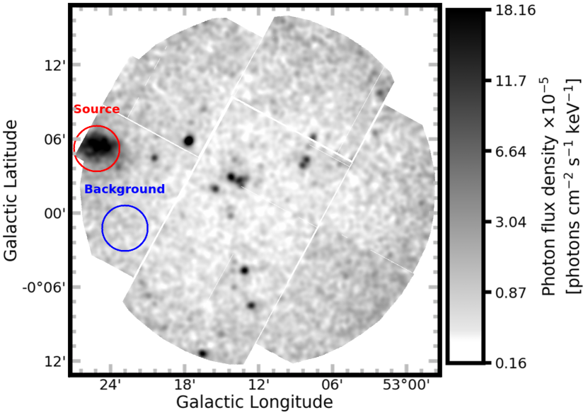
Figure 2: Exposure and vignetting corrected image from the XMM-Newton MOS2 detector. Source and background extraction regions are circled.

To perform the spectral analysis the SPEX fitting package version 3.04 (2017) together with SPEXACT 2.07 atomic tables were used (Kaastra et al., 1996). The fitting statistics method employed was C-statistics (Cash, 1979). Abundances were expressed with respect to Solar Abundance values of Lodders et al. (2009). For the emission measure parameter ($n_{\mathrm{e}}n_{\mathrm{H}}V$) we assumed a distance of $7.5\,\mathrm{kpc}$ (see Sec. 4.1). The analysis of the spectra was performed in the energy range between $0.7$ – $3.0\,\mathrm{keV}$, as this is the range in which the source spectrum dominates the background. The Obin command was used to obtain optimal binning of the spectra. After background subtraction the source spectrum consists of $\sim 2000$ counts. The spectrum was fit with a non-equilibrium ionization (NEI) model with Galactic absorption. The Galactic background was represented by the model hot in SPEX, with the temperature fixed to $0.5\,\mathrm{eV}$ to mimic absorption by neutral gas (de Plaa et al., 2016). The NEI model was employed with the following free parameters: electron temperature $T_{2}$, ionization age $\tau=n_{e}t$, normalization $n_{e}n_{H}V$, and abundances of elements Ne, Mg, Si, S, Fe. These elements have line emission in the energy band from $0.8$ – $2.6\mathrm{keV}$, the band for which there was sufficient signal to noise.

2.5 High-energy observations

We searched the High Energy Stereoscopic System CATalog (HESSCAT) and Third Fermi LAT Catalog of High-Energy Sources (3FGL; Acero et al., 2015) for high-energy sources associated with any of the SNR candidate shells. Fermi source 3FGL J1931.1+1659 is within the radius of SNR candidate $\mathrm{G}52.37-0.70$. There are no other high-energy sources close to the other five SNR candidates.

3 Results

The VGPS, WSRT, and LOFAR HBA observations of the six SNR candidates in the FoV – $\mathrm{G}51.21+0.11$, $\mathrm{G}52.37-0.70$, $\mathrm{G}53.07+0.49$, $\mathrm{G}53.41+0.03$, $\mathrm{G}53.84-0.75$, and $\mathrm{G}54.1+0.3$ – are shown in Figures 3 and 4. Only $\mathrm{G}53.41+0.03$ and $\mathrm{G}54.1+0.3$ have been observed in the X-ray band (see Sec. 2.4). As discussed by Anderson, et al. (2017), all six of the candidates have low thermal emission compared to the non-thermal emission, which we confirm using the MIPSGAL observations.

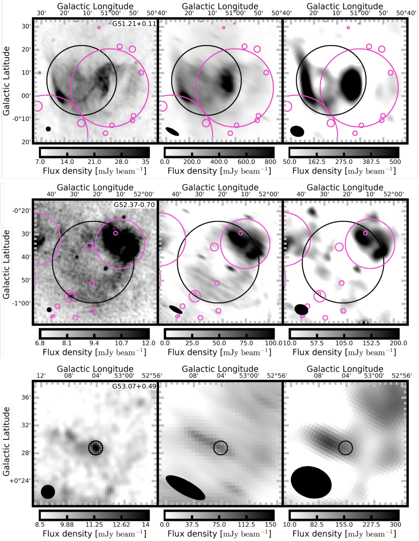
Figure 3: SNR candidates from Anderson, et al. (2017) in the FoV. In each row the left panel is the VGPS $1.4\,\mathrm{GHz}$ observation, the center panel is the WSRT $327\,\mathrm{MHz}$ observation, and the right panel is the LOFAR $144\,\mathrm{MHz}$ observation. From top to bottom the rows are the SNR candidates (circled in black) from Anderson, et al. (2017): $\mathrm{G}51.21+0.11$, $\mathrm{G}52.37-0.70$, and $\mathrm{G}53.07+0.49$. The magenta circles are HII regions from the WISE HII catalog (Anderson et al., 2014). The beam sizes are shown in the bottom left corner of each panel.

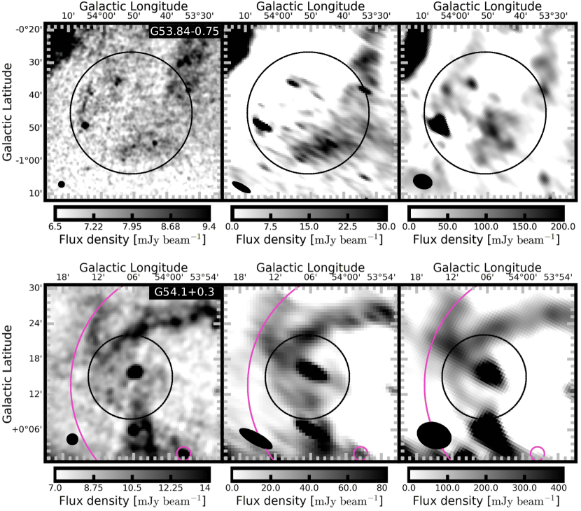
Figure 4: SNR candidates from Anderson, et al. (2017) in the FoV. In each row the left panel is the VGPS $1.4\,\mathrm{GHz}$ observation, the center panel is the WSRT $327\,\mathrm{MHz}$ observation, and the right panel is the LOFAR $144\,\mathrm{MHz}$ observation. From top to bottom the rows are the SNR candidates (circled in black) from Anderson, et al. (2017): $\mathrm{G}53.84-0.75$ and $\mathrm{G}54.1+0.3$. The magenta circles are HII regions from the WISE HII catalog (Anderson et al., 2014). The beam sizes are shown in the bottom left corner of each panel.

3.1 Radio results

The flux densities and spectral indices of SNR candidates $\mathrm{G}51.21+0.11$, $\mathrm{G}52.37-0.70$, $\mathrm{G}53.41+0.03$, and $\mathrm{G}53.84-0.75$, and the candidate shell around PWN $\mathrm{G}54.1+0.3$ measured using the positions and radii reported by Anderson, et al. (2017) are shown in Table 1. We subtracted the integrated flux density of the HII region overlapping $\mathrm{G}52.37-0.70$ and the flux density of the bright point source within $\mathrm{G}53.84-0.75$. Due to a drop-off in sensitivity away from the phase center of the HBA observation, we do not measure LOFAR integrated flux densities for $\mathrm{G}51.21+0.11$ and $\mathrm{G}52.37-0.70$.

	Flux density (Jy)
SNR	$1.4\,\mathrm{GHz}$	$327\,\mathrm{MHz}$	$150\,\mathrm{MHz}$	$\alpha$
G51.21+0.11	$24.35\pm 2.1$	$66.1\pm 0.1$		$-0.7\pm 0.21$
G52.37$-$0.70	$5.24\pm 1.75$	$3.2\pm 0.03$		$0.3\pm 0.3$
G53.41+0.03	$1.21\pm 0.21$	$2.2\pm 0.03$	$3.11\pm 0.2$	$-0.6\pm 0.2$
G53.84$-$0.75	$1.31\pm 3.43$	$0.06\pm 0.02$	$1.2\pm 0.07$	$0.05\pm 3.9$
G54.1+0.3	$1.46\pm 0.28$	$1.21\pm 0.05$	$0.4\pm 0.8$	$0.3\pm 4.3$

Table 1: Integrated flux densities of SNR candidates at $1.4\,\mathrm{GHz}$ from Anderson, et al. (2017), $327\,\mathrm{MHz}$ measured using WSRT observations (Taylor et al., 1996), and $150\,\mathrm{MHz}$ using LOFAR HBA observations. The WSRT errors are $3\sigma$ statistical errors based on the RMS noise in the image; these errors do not take other sources of error, such as confusion, into account. $\alpha$ was obtained using a simple power law and a weighted least squares fit using the measured error plus 20% for systematics. We note that a simple power law is not always the best model, for example for $\mathrm{G}54.1+0.3$.

SNR candidate $\mathrm{G}51.21+0.11$, shown in Figure. 3 (top row), has a complex morphology with a bright radio filament type structure and a bright radio patch. It has an HII region, $\mathrm{G}051.010+00.060$ (Anderson et al., 2014), on one side that appears to be coincident.

$\mathrm{52.37-0.70}$ is a faint radio shell visible most clearly in the VLA observation in the second row of Figure 3. There is a bright HII region, $\mathrm{G}052.174-00.567$ (Anderson et al., 2014), on the upper right of this candidate and some smaller HII regions within the shell.

$\mathrm{G}53.07+0.49$ has a small angular size (a radius of only $1^{\prime}$, Anderson, et al., 2017) and the location of the peak flux density is different for WSRT and LOFAR compared to the original VLA identification of the candidate. In Figure 3 (bottom panel) we can also see that there is some extended emission around $\mathrm{G}53.07+0.49$ that may or may not be associated with this candidate. As it is unclear which emission in the WSRT and LOFAR observations may or may not be associated with the candidate we do not measure WSRT or LOFAR flux densities for this candidate.

There is diffuse emission and some radio point sources in the region where candidate $\mathrm{G}53.84-0.75$ is located (Fig. 4, upper panel), but it is difficult to identify what emission is related to candidate $\mathrm{G}53.84-0.75$ and whether there is a discrete object or if the extended emission is Galactic Plane dust.

PWN $\mathrm{G}54.1+0.3$ is shown in Figure 4 (lower panel) where the bright spot in the center is the PWN and the partial loop around it is the known HII region $\mathrm{G}053.935+00.228$ (Anderson et al., 2014). There is some faint, diffuse radio emission around the PWN in the VLA observation, which is the SNR-shell candidate. In the WSRT and LOFAR observations of PWN $\mathrm{G}54.1+0.3$ shown in Figure 4 it appears that the possible shell identified in the VLA observations (Anderson, et al., 2017) fades away or is part of the surrounding HII region. The large uncertainty in the spectral index in Table 1 reflects that a powerlaw is not the best model; however, the flux density clearly decreases as the frequency decreases.

In the LOFAR HBA and VLA observations $\mathrm{G}53.41+0.03$ has a shell- or bubble-like morphology which is brighter on the upper edge, as shown in Figure 5. The radius of the shell at $144\,\mathrm{MHz}$ is $\sim 5^{\prime}$. As shown in Table 1 $\mathrm{G}53.41+0.03$ has a radio spectral index of $\alpha=-0.6\pm 0.2$.

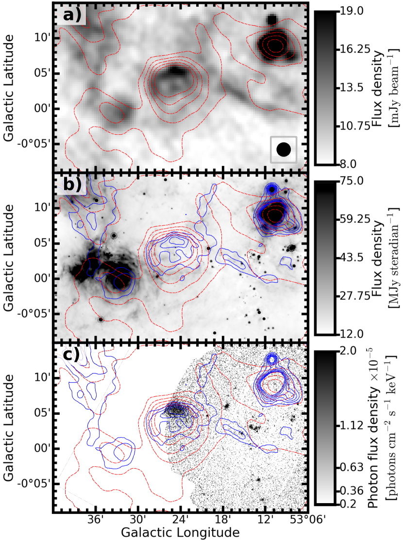
Figure 5: Observations of $\mathrm{G}53.41+0.03$ at (a) $1.4\,\mathrm{GHz}$ using the VLA, (b) $24.0\,\mathrm{\mu m}$ using Spitzer, and (c) X-rays using XMM-Newton. The dashed red contours are LOFAR HBA $144\,\mathrm{MHz}$ contours (contour levels: 0, 250, 500, 750, 1000 $\mathrm{mJy\,\,beam^{-1}}$) and the solid blue contours are VLA $1.4\,\mathrm{GHz}$ contours (contour levels: 12, 14, 16, 18, 20, 22, 24 $\mathrm{mJy\,\,beam^{-1}}$) from the image in (a). The VLA synthesised beam is shown in the bottom right corner of (a).

3.2 X-ray results

As described in Sec. 2.4, $\mathrm{G}53.84-0.75$ was observed by ROSAT. We used the PIMMS tool with the optically thin plasma model APEC with temperature $0.3\,\mathrm{keV}$ and local Galactic absorption value of $2.4\times 10^{22}$ cm^-2 to obtain the $2\sigma$ upper limit for the flux. No X-ray feature coincident to the radio observations was detected. The $2\sigma$ upper limit for the absorbed/unabsorbed flux is F${}_{0.4-2.4}\approx$ $2.4\times 10^{-13}$ / $4.1\times 10^{-11}$ erg s^-1 cm^-2.

The ROSAT and XMM-Newton X-ray observations of $\mathrm{G}53.41+0.03$ confirm the existence of an extended X-ray source at the location of $\mathrm{G}53.41+0.03$, particularly at the position of the radio-bright part of the shell. The XMM-Newton X-ray spectrum (Fig. 6) shows bright K-shell emission lines from magnesium, silicon, and sulfur and potential contributions from neon and iron around $1\,\mathrm{keV}$. This is typical of thermal emission from an optically thin plasma. The absorbed/unabsorbed flux of the source measured using XMM-Newton in the $0.7$ – $3.0\,\mathrm{keV}$ energy range is F$=7.3\times 10^{-13}$ / $3.1\times 10^{-11}$ erg s^-1 cm^-2. The best-fit NEI model is represented by a C-stat / d.o.f. of $83.48/64$. The parameters and $1\sigma$ errors are listed in Table 2, while the best fit model is shown in Figure 6. The ionization age informs us how far out of ionization equilibrium the plasma is, but given the narrow spectral range the parameter may correlate with the best-fit electron temperature $T_{2}$. To test the robustness of our best fit ionization age we calculate the error ellipse of $\tau$ and $T_{2}$, as shown in Figure 7.

Parameter	Unit	Value	Element	Abundance
NH	$10^{22}$ cm-2	2.4${}^{+0.2}_{-0.2}$	Ne	0.2${}^{+0.7}_{-0.2}$
nen${}_{H}V$	1057 cm-3	5${}^{+2}_{-2}$	Mg	0.9${}^{+0.3}_{-0.2}$
T2	keV	0.8${}^{+0.2}_{-0.1}$	Si	0.5${}^{+0.1}_{-0.1}$
$\tau$	$10^{10}$ s cm-2	4${}^{+2}_{-1}$	S	0.9${}^{+0.2}_{-0.2}$
			Fe	1.3${}^{+0.7}_{-0.5}$
Cstat/d.o.f				83.48/64

Table 2: XMM-Newton best-fit model results. The abundances are provided in Solar units.

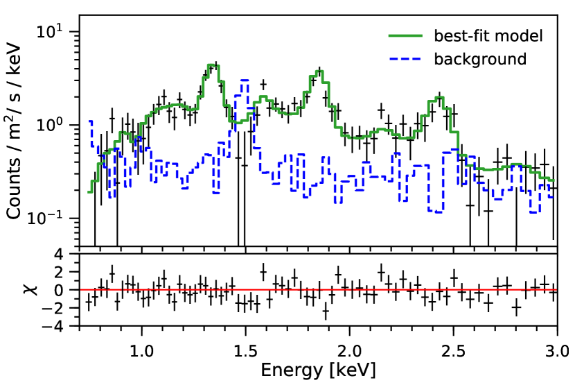
Figure 6: X-ray spectrum with the best-fit model and residuals.

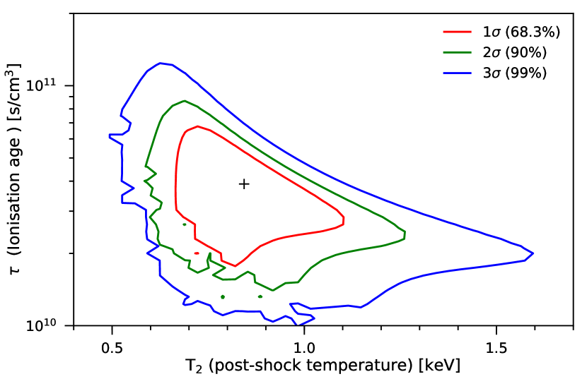
Figure 7: Contour plot of the ionization age and post-shock temperature. Best fit values are indicated by a small cross.

3.3 Radio pulsation search results

After performing a pulsation search as described in Sec. 2.2 we found no convincing astronomical signals in the data toward $\mathrm{G}53.41+0.03$, and we ascribe the statistically significant signals that we did detect to RFI.

Given the non-detection of radio pulsations toward $\mathrm{G}53.41+0.03$, we can place an upper limit on the integrated flux density of any associated radio pulsar. We use the modified radiometer equation (Dewey et al., 1985), and assume that interstellar scattering does not have a significant effect on broadening the pulses through multi-path propagation. While the central ALFA beam has a gain of $G\sim 10$ K Jy^-1, the 6 outer beams have $G\sim 8$ K Jy^-1. We targeted the center of $\mathrm{G}53.41+0.03$ (specifically, RA_J2000 = $19^{h}29^{m}57.41^{s}$, Dec_J2000 = $+18^{\circ}09^{\prime}53.5^{\prime\prime}$) in a $T=2400$-s pointing with the central ALFA beam, which covered a region of roughly 1.6^′ in radius. Since $\mathrm{G}53.41+0.03$ is roughly 10^′ wide, we also gridded a much larger $\sim 10^{\prime}$ wide region around $\mathrm{G}53.41+0.03$ in case the pulsar has moved from its birth site near the center of the SNR. In our sensitivity calculations we thus consider two scenarios: 1) where the pulsar is close to the center of $\mathrm{G}53.41+0.03$, and where we should use $G=10$ K Jy^-1 and $T=2400$ s and 2) a scenario in which the pulsar is offset by several arcminutes, and where $G=8$ K Jy^-1 and $T=900$ s. Furthermore, if the pulsar is located towards the half-power sensitivity point of one of the beams, then the effective sensitivity is also half. We make this conservative assumption for scenario 2.

The receiver temperature $T_{\rm rec}$ = 25 K and the sky temperature in this direction of the Galactic plane is $T_{\rm sky}$ = 5 K at 1400 MHz. We assume a W = 10% pulse duty cycle and a signal-to-noise S/N = 10 for detection. The two orthogonal linear polarizations, $n_{\rm p}$, of the receiver were summed, and the appropriate bandwidth is $\Delta\nu=172$ MHz. Finally, using the modified radiometer equation, and assuming no additional losses due to digitization, we find for scenario 1:

$$S^{1}_{\rm max}{\rm[mJy]}\frac{S/N(T_{\rm rec}+T_{\rm sky})}{G\sqrt{T\Delta\nu n_{\rm p}}}\sqrt{\frac{W}{(1-W)}}=0.011\,{\rm mJy}$$ (1)

For scenario 2, where the putative pulsar is more offset from $\mathrm{G}53.41+0.03$, $S^{2}_{\rm max}=0.045$ mJy. These are deep upper-limits on the flux density of any pulsar associated with $\mathrm{G}53.41+0.03$. Of the known young pulsars in the ATNF catalog, only a few have lower measured radio flux density (Manchester et al., 2005). However, because of beaming and the possibility of significant interstellar scattering, these limits do not definitively exclude a young pulsar associated with $\mathrm{G}53.41+0.03$.

4 Discussion

Here we will discuss the characteristics and nature of each SNR candidate. We will focus on $\mathrm{G}53.41+0.03$, including calculating its approximate distance and age.

G51.21$+$0.11: SNR candidate $\mathrm{G}51.21+0.11$ has a negative spectral index, $\alpha=-0.7\pm 0.21$, and a complex morphology coincident with a known HII region. There are no XMM-Newton or Chandra observations in the direction of the candidate to confirm its nature. We find $\mathrm{G}51.21+0.11$ to be an interesting object that is possibly an SNR, but further investigation using X-ray observations is required.

G52.37$-$0.70: Although $\mathrm{G}52.37-0.70$ has a shell-like morphology in the VLA observations, it has a spectral index of $\alpha=0.3\pm 0.3$ fitted using the VLA and WSRT integrated flux densities. The spectral index indicates that this candidate is unlikely to be an SNR, and as such the Fermi source within the radius of the candidate (see Sec. 2.5) is unlikely to be associated.

G53.07$+$0.49: Candidate $\mathrm{G}53.07+0.49$ has a small angular size in the VLA observations, but the peak flux density in the WSRT and LOFAR observations is offset from the SNR candidate location suggested by (Anderson, et al., 2017). As such we do not measure WSRT or LOFAR flux densities for this candidate, and as there are no X-ray observations available, further investigation using X-ray or higher resolution low-frequency observations is required to comment on the nature of this candidate.

G53.84$-$0.75: It is not clear what emission is SNR candidate $\mathrm{G}53.84-0.75$ and there are large errors on the VLA integrated flux density from Anderson, et al. (2017). This, as well as the strange spectral shape, suggests that there is no discrete, extended object at this position. This is supported by the ROSAT X-ray non-detection. For this reason we find it unlikely that $\mathrm{G}53.84-0.75$ is an SNR.

G54.1$+$0.3: Whether PWN $\mathrm{G}54.1+0.3$ has an SNR shell has been in question since Lang et al. (2010) found faint radio emission around the PWN, which is just visible in the VLA observation (Fig. 4). Lu et al. (2002) found no evidence of a shell in their Chandra observations, while Bocchino et al. (2010) found hints of a very faint, diffuse shell using Suzaku and XMM-Newton. Anderson, et al. (2017) find that the shell suggested by Lang et al. (2010) is more likely to be part of the surrounding HII region. Alternatively, Anderson, et al. (2017) suggest a slightly smaller radius shell ($7.2^{\prime}$) as a possible shell around PWN $\mathrm{G}54.1+0.3$ with an integrated flux density of $1.46\,\mathrm{Jy}$ at $1.4\,\mathrm{GHz}$. There is no evidence for extended emission around PWN $\mathrm{G}54.1+0.3$ in our LOFAR HBA observation, as can be seen in Figure 4 (bottom panel), aside from the known HII region $\mathrm{G}053.935+0.228$ (Anderson et al., 2014). This is supported by the low flux-densities measured by WSRT and LOFAR (shown in Table 1) using a region of radius $7.2^{\prime}$ and subtracting the flux density of the PWN. We find it unlikely that there is a shell around PWN $\mathrm{G}54.1+0.3$.

G53.41$+$0.03: $\mathrm{G}53.41+0.03$ has a morphology common to SNRs. Using the flux densities shown in Table 1 we find that the $\mathrm{G}53.41+0.03$ has a steep negative radio spectral index, $\alpha=-0.6\pm 0.2$, as expected for an SNR. X-ray analysis indicates that the plasma of $\mathrm{G}53.41+0.03$ has a relatively high temperature of $\mathrm{T}_{2}\sim 0.8\,\mathrm{keV}$. The ionization age $\tau\sim 10^{10.6}\,\mathrm{s}\cdot\mathrm{cm}^{-3}$ is much lower than needed for ionization/recombination balance ($\tau\geq 10^{12}\,\mathrm{s}\cdot\mathrm{cm}^{-3}$). The fact that the spectrum is far out of ionization equilibrium is a clear signature that the source is an SNR (Vink, 2012), as no other known source class has gas tenuous enough and/or is young enough to be far out of ionization equilibrium. We therefore confirm that $\mathrm{G}53.41+0.03$ is an SNR, and further investigate it by calculating its approximate distance and age.

4.1 The distance to G53.41+0.03

Estimating the distance to Galactic SNRs is notoriously difficult. There are few methods that give reliable results, such as kinematic methods, based on optical Doppler shifts combined with proper motion of optical filaments (e.g. Reed et al., 1995, for Cas A), or, less reliably, 21cm line absorption combined with a Galactic rotation model (see e.g. Roman-Duval et al., 2009; Kothes & Foster, 2012, for an explanation and SNR application of the model). In contrast, SNRs located in the Magellanic Clouds can be reliably placed at the distance of these satellite galaxies. By using reliable distance estimates some secondary distance indicators have been developed, such as the X-ray Galactic absorption column (Strom, 1994) and the $\mathrm{\Sigma-D}$ relation (Pavlovic et al., 2014).

A first indication of the distance of an SNR can be its positional association with a spiral arm. However, the reason that the investigated field is so rich in sources is that the line of sight crosses the Sagittarius-Carina arm tangentially as well as regions of the Perseus arm. Taking the Galactic spiral arm model of Hou et al. (2009), we find that the $l=53.4^{\circ}$ line of sight intercepts the Sagittarius arm (arm -3 in Hou et al., 2009) between $\sim 4$ kpc and 7.5 kpc, and the Perseus arm at 9.6 kpc. Given that the Sagittarius arm is tangential along the line of sight, this suggests a probable distance between 4.5 and 7.5 kpc.

Strom (1994) derived a relation between column density and distance of $N_{\mathrm{H}}=8.4\times 10^{21}d^{1.58}$ cm^-2. The measured column density of $N_{\mathrm{H}}=2.4\times 10^{22}$ cm^-2 (Table 2), therefore, suggests a distance of $\sim 8.4$ kpc. However, one should be cautious here, because the line of sight crosses the arm tangentially, which is likely to lead to a column density that is higher than average for a given distance.

The surface brightness of $\mathrm{G}53.41+0.03$ normalized to 1 GHz is $\Sigma=8.3\times 10^{-21}$ W m^-2 Hz^-1sr^-1. The $1\,\mathrm{GHz}$ surface brightness was obtained using the $1.4\,\mathrm{GHz}$ flux density measured by Anderson, et al. (2017) and a spectral index of $\alpha=-0.6$ (see Tab. 1). Using the relation between diameter and surface brightness (the $\mathrm{\Sigma-D}$ relation) in Pavlovic et al. (2014) gives yet another distance estimate of $8\,\mathrm{kpc}$. However, we know that the $\mathrm{\Sigma-D}$ relation is controversial, as there is large scatter which may relate to the SNR environments, and there is debate on the statistical validity of the relation (e.g. Arbutina & Urošević, 2005; Filipović et al., 2005; Green, 2014).

The distance estimates based on the X-ray absorption and $\mathrm{\Sigma-D}$ relation, although uncertain, are consistent with the idea that the SNR is located in the Sagittarius-Carina arm, but suggest that the SNR is on the far-side of the arm. We therefore adopt a distance of $7.5\,\mathrm{kpc}$ for $\mathrm{G}53.41+0.03$. The angular radius of $\sim 5^{\prime}$ translates then into a physical radius of 10.7$d_{7.5}$ pc, with $d_{7.5}$ the distance in units of $7.5\,\mathrm{kpc}$.

4.2 The age of G53.41+0.03

The spectrum of $\mathrm{G}53.41+0.03$ allows us to put some constraints on the density and age of the SNR. To do this we need a volume estimate. Given a typical volume filling fraction of 25% and assuming a spherical morphology, we estimate the volume to be $V_{\mathrm{SNR}}=3.3\times 10^{58}d_{7.5}^{3}$ cm³. The X-ray spectrum was obtained for only $\sim 20$% of the shell, so we take $V_{\mathrm{X}}\approx 6.7\times 10^{57}d_{7.5}^{3}$ cm³ to be the volume pertaining to the X-ray spectrum. Taking $n_{\mathrm{e}}\approx 1.2n_{H}$ in the emission measure $n_{\mathrm{e}}n_{H}V$, we obtain the density $n_{\mathrm{H}}\approx 0.8d_{7.5}^{-3/2}$ cm^-3. Using this number together with the best-fit ionization age of $n_{\mathrm{e}}t=4\times 10^{10}$ cm^-3s we find an approximate age of 1600$d_{7.5}^{3/2}$ yr.

The measured electron temperature corresponds to a shock velocity of $V_{\mathrm{s}}\approx 800$ km s^-1 or higher if the electron temperature is lower than the ion temperature (Vink, 2012). For the Sedov-Taylor self-similar evolution model we have $V_{\mathrm{s}}=0.4R/t$.Using $R=10.7d_{7.5}$ pc, gives then an approximate age of $\sim 5300d_{7.5}$ yr. Using the Sedov-Taylor evolution model of $R^{5}=2.026Et^{2}/\rho$, with $E=10^{51}$ erg gives yet another estimate of the age of $\sim 7800d_{7.5}^{7/4}$ yr. The two estimates based on the Sedov-Taylor model give roughly similar results for the canonical explosion energy of $10^{51}$ erg ($t\approx 6500\pm 1500$ yr), whereas the estimate based on the ionization age suggests a younger age. This discrepancy may be due to non-standard evolution scenarios, for example evolution in a wind-blow cavity. This needs to be addressed in follow-up studies. However, these estimates agree that $\mathrm{G}53.41+0.03$ is an SNR with an age somewhere between 1000 and 8000 yr. X-ray observations centered on and covering the whole SNR are needed to fully characterize the properties of $\mathrm{G}53.41+0.03$.

5 Conclusion

We confirm that SNR candidate, $\mathrm{G}53.41+0.03$, is in fact an SNR using XMM-Newton observations, and LOFAR observations targeting PWN $\mathrm{G}54.1+0.3$. $\mathrm{G}53.41+0.03$ has a shell-like morphology in the radio, with a radius of $\sim 5\,^{\prime}$. Using LOFAR HBA observations, as well as archival WSRT and VGPS mosaics, we confirm that $\mathrm{G}53.41+0.03$ has a steep spectral index ($\alpha=-0.6\pm 0.2$), typical of synchrotron radiation from SNRs. MIPSGAL observations show that $\mathrm{G}53.41+0.03$ has no IR component. Archival XMM-Newton observations show that $\mathrm{G}53.41+0.03$ has an associated X-ray component with a coincident morphology to the radio shell. Furthermore, analysis and fitting of the XMM-Newton observation show that $\mathrm{G}53.41+0.03$ has strong emission lines and is best characterized by a non-equilibrium ionization model, with an ionization age and normalization typical for an SNR with an age between 1000 and 8000 yr and a density of $n_{\mathrm{H}}\approx 0.8d_{7.5}^{-3/2}$ cm^-3. Given the X-ray, IR, and radio characteristics of $\mathrm{G}53.41+0.03$, we confirm that it is a new Galactic Plane SNR. We do not find a pulsar associated with $\mathrm{G}53.41+0.03$, but the upper-limits on the flux density do not exclude the possibility of a young pulsar that is exceptionally weak or not beamed towards Earth.

We also investigate five other SNR candidates from Anderson, et al. (2017) in the same LOFAR FoV. We show that three of these candidates ($\mathrm{G}52.37-0.70$, $\mathrm{G}53.84-0.75$ and the shell around PWN $\mathrm{G}54.1+0.3$) are unlikely to be SNRs and one, $\mathrm{G}51.21+0.11$, is a good SNR candidate that requires further investigation. This demonstrates that it is important to further investigate SNR candidates using low-frequency observations with telescopes such as WSRT and LOFAR.

References

- Acero et al. (2015) Acero, F., Ackermann, M., Ajello, M., et al. 2015, ApJS, 218, 23
- Anderson et al. (2014) Anderson, L. D., Bania, T. M., Balser, D. S., et al. 2014, Astrophysical Journal, Supplement, 212, 1
- Anderson, et al. (2017) Anderson, L. D., Wang, Y., Bihr, S., et al. 2017, A&A, 605, A58.
- Arbutina & Urošević (2005) Arbutina, B., & Urošević, D. 2005, MNRAS, 360, 76
- Astropy Collaboration et al. (2013) Astropy Collaboration, Robitaille, T. P., Tollerud, E. J., et al. 2013, A&A, 558, A33
- Bocchino et al. (2010) Bocchino, F., Bandiera, R., & Gelfand, J. 2010, A&A, 520, A71
- Briggs (1995) Briggs, D. S. 1995, Bulletin of the American Astronomical Society, 27, 112.02
- Brogan et al. (2006) Brogan, C. L., Gelfand, J. D., Gaensler, B. M., Kassim, N. E., & Lazio, T. J. W. 2006, ApJ, 639, L25
- Carey et al. (2009) Carey, S. J., Noriega-Crespo, A., Mizuno, D. R., et al. 2009, Publications of the Astronomical Society of Pacific, 121, 76
- Cash (1979) Cash, W. 1979, The Astrophysical Journal, 228, 939
- Caswell (1985) Caswell, J. L. 1985, Astrophyical Journal, 90, 1224
- Day et al. (1972) Day, G. A., Caswell, J. L., & Cooke, D. J. 1972, Australian Journal of Physics Astrophysical Supplement, 25, 1
- de Plaa et al. (2016) de Plaa, J., Ebrero, J., Grange, Y., et al. 2016, SPEX Cookbook
- Dewey et al. (1985) Dewey, R. J., Taylor, J. H., Weisberg, J. M., & Stokes, G. H. 1985, ApJ, 294, L25
- Filipović et al. (2005) Filipović, M. D., Payne, J. L., Reid, W., et al. 2005, MNRAS, 364, 217
- Gerbrandt et al. (2014) Gerbrandt, S., Foster, T. J., Kothes, R., Geisbüsch, J., & Tung, A. 2014, A&A, 566, A76
- Gottschall et al. (2016) Gottschall, D., Capasso, M., Deil, C., et al. 2016, ArXiv e-prints, arXiv:1612.00261 [astro-ph.HE]
- Green (2005) Green, D. A. 2005, Mem. Soc. Astron. Italiana, 76, 534
- Green (2014) —. 2014, Bulletin of the Astronomical Society of India, 42, 47
- Green (2017) —. 2017, VizieR Online Data Catalog, 7278 https://www.mrao.cam.ac.uk/surveys/snrs/
- Gutermuth & Heyer (2015) Gutermuth, R. A., & Heyer, M. 2015, The Astronomical Journal, 149, 64
- Hou et al. (2009) Hou, L. G., Han, J. L., & Shi, W. B. 2009, A&A, 499, 473
- Intema et al. (2017) Intema, H. T., Jagannathan, P., Mooley, K. P., & Frail, D. A. 2017, Astronomy & Astrophysics, 598, A78
- Kaastra et al. (1996) Kaastra, J. S., Mewe, R., & Nieuwenhuijzen, H. 1996, UV and X-ray Spectroscopy of Astrophysical and Laboratory Plasmas, 411
- Kim et al. (2013) Kim, H.-J., Koo, B.-C., & Moon, D.-S. 2013, The Astrophysical Journal, 774, 5
- Kothes & Foster (2012) Kothes, R., & Foster, T. 2012, ApJ, 746, L4
- Kothes et al. (2017) Kothes, R., Reich, P., Foster, T. J., & Reich, W. 2017, A&A, 597, A116
- Lang et al. (2010) Lang, C. C., Wang, Q. D., Lu, F., & Clubb, K. I. 2010, The Astrophysical Journal, 709, 1125
- Li et al. (1991) Li, Z., Wheeler, J. C., Bash, F. N., & Jefferys, W. H. 1991, The Astrophysical Journal, 378, 93
- Lodders et al. (2009) Lodders, K., Palme, H., & Gail, H. P. 2009, arXiv:0901.1149
- Lu et al. (2002) Lu, F. J., Wang, Q. D., Aschenbach, B., Durouchoux, P., & Song, L. M. 2002, ApJ, 568, L49
- Manchester et al. (2005) Manchester, R. N., Hobbs, G. B., Teoh, A., & Hobbs, M. 2005, AJ, 129, 1993
- Matthews et al. (1998) Matthews, B. C., Wallace, B. J., & Taylor, A. R. 1998, The Astrophysical Journal, 493, 312
- Offringa et al. (2014) Offringa, A. R., McKinley, B., Hurley-Walker, et al. 2014, Monthly Notices of the Royal Astronomical Society, 444, 606
- Onić (2013) Onić, D. 2013, Astrophysics and Space Science, 346, 3
- Pavlovic et al. (2014) Pavlovic, M. Z., Dobardzic, A., Vukotic, B., & Urosevic, D. 2014, Serbian Astronomical Journal, 189, 25
- Reed et al. (1995) Reed, J. E., Hester, J. J., Fabian, A. C., & Winkler, P. F. 1995, ApJ, 440, 706
- Robitaille & Bressert (2012) Robitaille, T., & Bressert, E. 2012, APLpy: Astronomical Plotting Library in Python, Astrophysics Source Code Library, ascl:1208.017
- Roman-Duval et al. (2009) Roman-Duval, J., Jackson, J. M., Heyer, M., et al. 2009, ApJ, 699, 1153
- Stil et al. (2006) Stil, J. M., Taylor, A. R., Dickey, J. M., et al. 2006, The Astronomical Journal, 132, 1158
- Strom (1994) Strom, R. G. 1994, Monthly Notices of the Royal Astronomical Society, 268, L5
- Strom (1994) Strom, R. G. 1994, A&A, 288, L1
- Tammann et al. (1994) Tammann, G. A., Loeffler, W., & Schroeder, A. 1994, ApJS, 92, 487
- Taylor et al. (1996) Taylor, A. R., Goss, W. M., Coleman, P. H., van Leeuwen, J., & Wallace, B. J. 1996, The Astrophysical Journal, 107, 239
- Turner et al. (2001) Turner, M. J. L., Abbey, A., Arnaud, M., et al. 2001, Astronomy & Astrophysics, 365, L27
- Van Der Walt et al. (2011) Van Der Walt, S., Colbert, S. C., & Varoquaux, G. 2011, ArXiv e-prints, arXiv:1102.1523 [cs.MS]
- van Haarlem et al. (2013) van Haarlem, M. P., Wise, M. W., Gunst, A. W., et al. 2013, A&A, 556, A2
- van Weeren et al. (2016) van Weeren, R. J., Williams, W. L., Hardcastle, M. J., et al. 2016, The Astrophysical Journal Supplement Series, 223, 2
- Vink (2012) Vink, J. 2012, The Astronomy and Astrophysics Review, 20, 49