The pulsating magnetosphere of the extremely slowly rotating magnetic $\beta$ Cep star $\xi^{1}$ CMa

Abstract

$\xi^{1}$ CMa is a monoperiodically pulsating, magnetic $\beta$ Cep star with magnetospheric X-ray emission which, uniquely amongst magnetic stars, is clearly modulated with the star’s pulsation period. The rotational period $P_{\rm rot}$ has yet to be identified, with multiple competing claims in the literature. We present an analysis of a large ESPaDOnS dataset with a 9-year baseline. The longitudinal magnetic field $\langle B_{z}\rangle$ shows a significant annual variation, suggesting that $P_{\rm rot}$ is at least on the order of decades. The possibility that the star’s H$\alpha$ emission originates around a classical Be companion star is explored and rejected based upon VLTI AMBER and PIONIER interferometry, indicating that the emission must instead originate in the star’s magnetosphere and should therefore also be modulated with $P_{\rm rot}$. Period analysis of H$\alpha$ EWs measured from ESPaDOnS and CORALIE spectra indicates $P_{\rm rot}>30$ yr. All evidence thus supports that $\xi^{1}$ CMa is a very slowly rotating magnetic star hosting a dynamical magnetosphere. H$\alpha$ also shows evidence for modulation with the pulsation period, a phenomenon which we show cannot be explained by variability of the underlying photospheric line profile, i.e. it may reflect changes in the quantity and distribution of magnetically confined plasma in the circumstellar environment. In comparison to other magnetic stars with similar stellar properties, $\xi^{1}$ CMa is by far the most slowly rotating magnetic B-type star, is the only slowly rotating B-type star with a magnetosphere detectable in H$\alpha$ (and thus, the coolest star with an optically detectable dynamical magnetosphere), and is the only known early-type magnetic star with H$\alpha$ emission modulated by both pulsation and rotation.

1 Introduction

The bright ($V=4.3$ mag), sharp-lined $\beta$ Cep pulsator $\xi^{1}$ CMa (HD 46328, B0.5 IV) was first reported to be magnetic by Hubrig et al. (2006), based upon FORS observations at the Very Large Telescope (VLT). Silvester et al. (2009) confirmed the detection using ESPaDOnS at the Canada-France-Hawaii Telescope (CFHT).

Despite intensive observation campaigns with different spectropolarimeters, there are conflicting claims regarding the star’s rotational period: Hubrig et al. (2011) derived a rotational period of $\sim$2.18 d based on FORS1/2 and SOFIN data, while Fourtune-Ravard et al. (2011) found a longer period of $\sim$4.27 d based on ESPaDOnS measurements. Both Hubrig et al. and Fourtune-Ravard et al. agreed that the star was likely being viewed with a rotational pole close to the line of sight. However, Fourtune-Ravard et al. noted that given the small variation in $\langle B_{z}\rangle$ they could not rule out intrinsically slow rotation.

Frost (1907) was the first to note $\xi^{1}$ CMa’s variable radial velocity. McNamara (1955) found a pulsation period of $\sim$0.2 d, identifying the star as a $\beta$ Cephei variable. While many $\beta$ Cep stars are multi-periodic, $\xi^{1}$ CMa appears to be a monoperiodic pulsator (Saesen et al., 2006) with an essentially constant period (Jerzykiewicz, 1999). In their analysis of CORALIE high-resolution spectroscopy, Saesen et al. (2006) found a pulsation period of 0.2095764(4) d (where the number in brackets refers to the uncertainty in the final digit). Saesen et al. also reported that $\xi^{1}$ CMa is one of the few $\beta$ Cep stars that achieves supersonic pulsation velocities. Several spectroscopic mode identification methods revealed that the oscillation frequency most likely corresponds to either a radial $(l,m)=(0,0)$ mode, or a dipolar $(l,m)=(1,0)$ mode, the latter viewed at small inclination. An $l=2$ mode was ruled out via modelling of the velocity moments. Photometric mode identification indicates that only the radial mode agrees with the frequency (Heynderickx et al., 1994).

Like many magnetic early-type stars, $\xi^{1}$ CMa displays the emission signatures of a magnetized stellar wind in optical, ultraviolet, and X-ray spectra. The star’s X-ray emission spectrum is very hard, and the brightest amongst all magnetic $\beta$ Cep stars, as demonstrated with Einstein (Cassinelli et al., 1994), ROSAT (Cassinelli et al., 1994), and XMM-Newton (Oskinova et al., 2011). The star’s X-ray emission has recently been shown to be modulated with the pulsation period (Oskinova et al., 2014), a so-far unique discovery amongst massive magnetic pulsators (Favata et al., 2009; Oskinova et al., 2015). Various wind-sensitive ultraviolet lines show strong emission (Schnerr et al., 2008), which is typical for magnetic stars. $\xi^{1}$ CMa has also been reported to display H$\alpha$ emission (Fourtune-Ravard et al., 2011), although the properties of this emission have not yet been investigated in detail.

Our goals in this paper are, first, to determine the rotational period based upon an expanded ESPaDOnS dataset, and second, to examine the star’s H$\alpha$ emission properties.

The observations are presented in § 2. In § 3 we refine the pulsation period using radial velocity measurements. In § 4 we analyze the line broadening, determine the stellar parameters, and investigate the relationship between the star’s pulsations and its effective temperature. In § 5 we examine the possibility that the H$\alpha$ emission may be a consequence of an undetected binary companion, constraining the brightness of such a companion using both interferometry and radial velocity measurements. The magnetic measurements and magnetic period analysis are presented in § 6. We examine the long- and short-term variability of the H$\alpha$ emission in § 7, and investigate the influence of pulsation on wind-sensitive UV resonance lines. Magnetic and magnetospheric parameters are determined in § 8, § 9 presents a discussion of the paper’s results, and the conclusions are summarized in § 10.

2 Observations

2.1 ESPaDOnS spectropolarimetry

Under the auspices of the Magnetism in Massive Stars (MiMeS) CFHT Large Program (Wade et al., 2016), 29 ESPaDOnS Stokes $V$ spectra were acquired between 2008/01 and 2013/02. One additional observation was already published by Silvester et al. (2009). A further 4 ESPaDOnS observations were acquired by a PI program in 2014, and another 22 by a separate PI program in 2017. ESPaDOnS is a fibre-fed echelle spectropolarimeter, with a spectral resolution $\lambda/\Delta\lambda\sim 65,000$, and a spectral range from 370 to 1050 nm over 40 spectral orders. Each observation consists of 4 polarimetric sub-exposures, between which the orientation of the instrument’s Fresnel rhombs are changed, yielding 4 intensity (Stokes $I$) spectra, 1 circularly polarized (Stokes $V$) spectrum, and 2 null polarization ($N$) spectra, the latter obtained in such a way as to cancel out the intrinsic polarization of the source. The majority of the data were acquired using a sub-exposure time of 60 s, with the exception of the first observation (75 s), and the data acquired in 2017, for which a 72 s sub-exposure time was used to compensate for degradation of the coating of CFHT’s mirror. The data were reduced using CFHT’s Upena reduction pipeline, which incorporates Libre-ESPRIT, a descendent of the ESPRIT code described by Donati et al. (1997). Wade et al. (2016) describe the reduction and analysis of MiMeS ESPaDOnS data in detail.

The log of ESPaDOnS observations is provided in an online Appendix in Table B4. The quality of the data is excellent, with a median peak signal-to-noise ratio (S/N) per spectral pixel of 828 in the combined Stokes $V$ spectrum. The 2 observations acquired on 2017/02/11 had a peak S/N below 500, and were discarded from the magnetic analysis. The log of sub-exposures, which were used for spectroscopic analysis, is provided in an online Appendix in Table C6. Note that while there are 56 full polarization sequences, due to one incomplete polarization sequence there are 227 rather than 224 sub-exposures listed in Table C6.

2.2 MuSiCoS spectropolarimetry

Three Stokes $V$ spectra were obtained in 2000/02 with the MuSiCoS spectropolarimeter on the Bernard Lyot Telescope (TBL) at the Pic du Midi Observatory. This instrument, one of several similar fibre-fed échelle multi-site continuous spectroscopy (hence MuSiCoS) instruments (Baudrand & Bohm, 1992) constructed at various observatories was uniquely coupled to a polarimeter (Baudrand & Bohm, 1992; Donati et al., 1999). It had a spectral resolution of 35,000 and covered the wavelength range 450–660 nm, across 40 spectral orders. As with ESPaDOnS, each polarimetric sequence consisted of 4 polarized subexposures, from which Stokes $I$ and $V$ spectra, as well as a diagnostic null $N$ spectrum, were extracted. The log of MuSiCoS data is provided in an online Appendix in Table B4. One of the MuSiCoS observations has a low S/N (below 100), and was discarded from the analysis. The data were reduced using ESPRIT (Donati et al., 1997).

Normal operation of the instrument was verified by observation of magnetic standard stars in the context of other observing programs (Shorlin et al., 2002; Kochukhov et al., 2004; Wade et al., 2006). In addition to this, we utilize the MuSiCoS spectra of 36 Lyn presented by Wade et al. (2006), one of which was obtained during the same observing run as those of $\xi^{1}$ CMa, in order to compare them to observations of the same star acquired recently with Narval, a clone of ESPaDOnS which replaced MuSiCoS at TBL, and which achieves essentially identical results (Wade et al., 2016). This comparison is provided in Appendix A.

2.3 CORALIE optical spectroscopy

A large dataset (401 spectra) was obtained between 2000/02 and 2004/10 with the CORALIE fibre-fed echelle spectrograph installed at the Nasmyth focus of the Swiss 1.2 m Leonard Euler telescope at the European Southern Observatory’s (ESO) La Silla facility (Queloz et al., 2000, 2001). The spectrograph has a spectral resolving power of $\sim$100,000, and covers the wavelength range 387–680 nm across 68 spectral orders. The data were reduced with TACOS (Baranne et al., 1996). The first analysis of these data was presented by Saesen et al. (2006).

The log of CORALIE observations is provided in an online Appendix in Table C10. The median peak S/N is 205. One observation, acquired on 10/12/2003, was discarded as it had a S/N of 16, too low for useful measurements.

2.4 IUE ultraviolet spectroscopy

$\xi^{1}$ CMa was observed numerous times with the International Ultraviolet Explorer (IUE). The IUE could operate in two modes, high-dispersion ($R\sim 2000$) or low-dispersion ($R\sim 300$), with two cameras, the Short Wavelength (SW) from 115 to 200 nm and the Long Wavelength (LW) from 185 to 330 nm. We retrieved the data from the MAST archive. The data were reduced with the New Spectral Image Processing System (NEWSIPS). There are two simultaneous low-resolution spectra obtained with the Short Wavelength Prime (SWP) and Long Wavelength Redundant (LWR) cameras, along with 13 high-resolution spectra obtained with the SWP camera. The high-resolution data are of uniform quality as measured by the S/N, which is approximately 20 in all cases. Twelve of the spectra were obtained in close temporal proximity, covering a single pulsation cycle in approximately even phase intervals. The first observation was obtained 154 days previously. We used the absolute calibrated flux, discarded all pixels flagged as anomalous, and merged the various spectral orders.

2.5 VLTI near infrared interferometry

While the angular radii of $\xi^{1}$ CMa and its circumstellar material are certainly too small to be resolved interferometrically, the star is bright enough that the data can be used to search for a high-contrast binary companion.

We have acquired four Very Large Telescope Interferometer (VLTI) observations: low-resolution AMBER H and K photometry, a high-resolution AMBER NIR spectro-interferogram, and one low-resolution H band PIONIER observation. AMBER (Astronomical Multi-Beam Recombiner) offers three baselines and can operate in either low-resolution photometric mode or high-resolution ($R\sim 12000$) spectro-interferometric mode (Petrov et al., 2007). PIONIER (Precision Integrated-Optics Near-infrared Imaging ExpeRiment) combines light from 4 telescopes, offering visibilities across 6 baselines together with 4 closure phase measuremnts (Le Bouquin et al., 2011). All data were obtained using the 1.8 m Auxilliary Telescopes (ATs), which have longer available baselines, and hence better angular resolution than the 8 m Unit Telescopes (UTs). AMBER observations were obtained with baselines ranging from 80 to 129 m. PIONIER was configured in the large quadruplet, with a longest baseline of 140 m. The nearby star $\xi^{2}$ CMa (A0 III, $H=4.63$) was used as a standard star for calibration.

The observing log is given in Table D17. As the execution time for a full measurement ($\sim$1 hr) is a significant fraction of the pulsation period, pulsation phases are not given.

Owing to the relatively faint magnitude, the wavelength edges of the AMBER H and K profiles were particularly noisy. These data points were edited out by hand before commencing the analysis. No such procedure was necessary for the PIONIER observation.

3 Pulsation Period

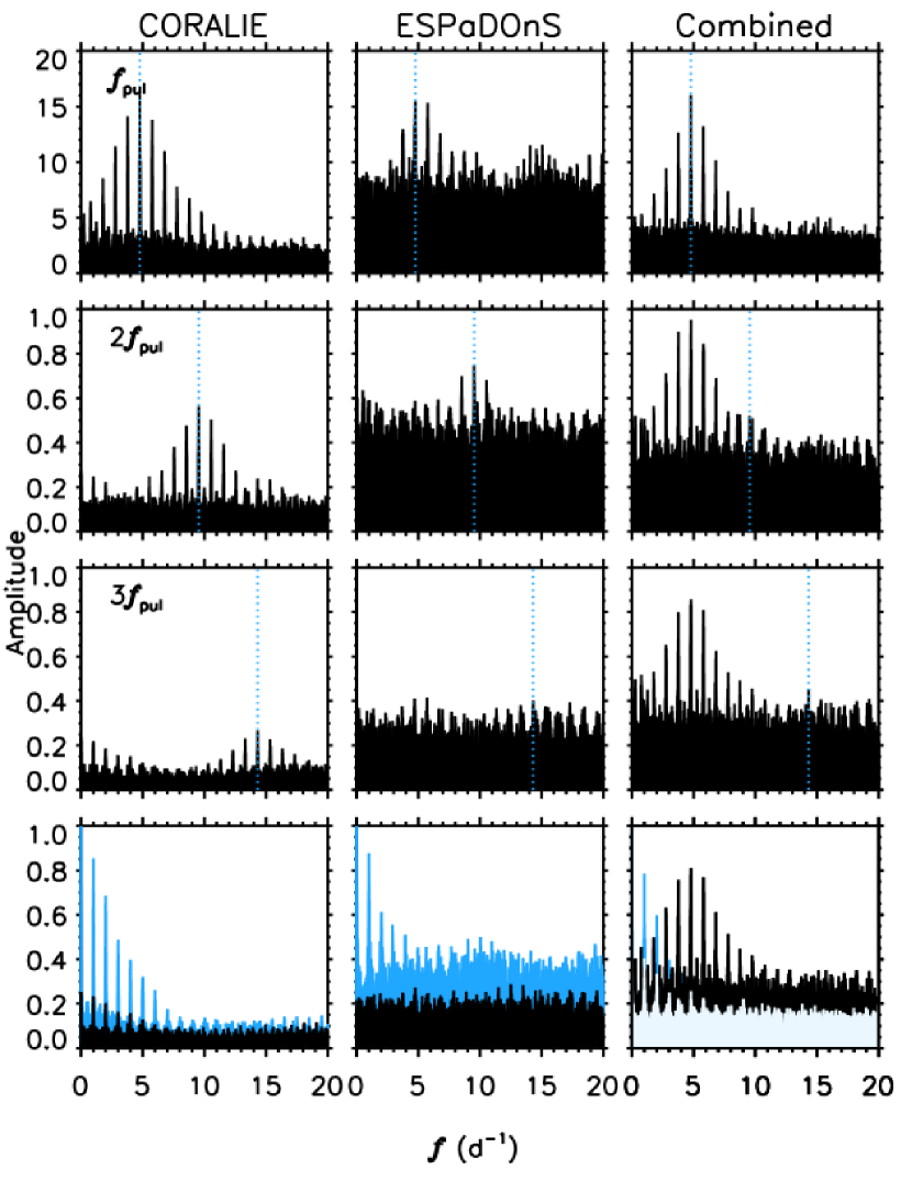
Figure 1: Frequency spectra for radial velocities (RVs) measured from CORALIE data (left), ESPaDOnS data (middle), and the combined (right) dataset, for the RVs (top row), and after pre-whitening with significant frequencies (subsequent rows). Dotted light blue lines indicate $f_{\rm pul}\sim 4.77153~{}{\rm d}^{-1}$ and its first two harmonics. In the bottom panels, the window function is overplotted in light blue. In the bottom right panel, the white frequency spectrum shows the results of prewhitening the combined data with a pulsation period increasing at a linear rate of $0.0096(5){\rm s}~{}{\rm yr}^{-1}$. By contrast, using a constant period to prewhiten the combined dataset (black frequency spectrum) does not fully remove the peak at $f_{\rm pul}$.

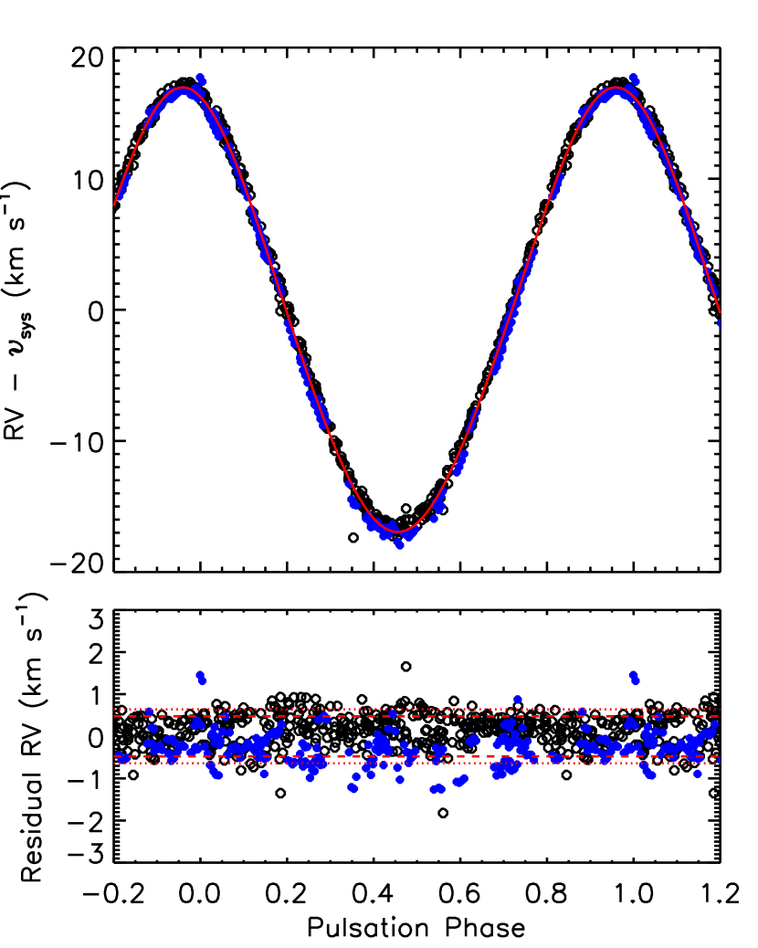
Figure 2: Top panel: Composite radial velocities (using N II 404.4 and 422.8 nm; N III 463.4 nm; O II 407.2, 407.9, 418.5, and 445.2 nm; Ne II 439.2 nm; Al III 451.3 nm; Si iii 455.3 nm; and Si IV 411.6 nm) as a function of pulsation phase, using the nonlinear ephemeris defined in Eqn. 1. Open black circles are CORALIE measurements, filled blue circles ESPaDOnS measurements. The solid red line indicates a $3^{rd}$-order sinusoidal fit. Bottom panel: residual radial velocities. Dashed red lines indicate $\pm$1 standard deviation, about 0.48 km s^-1, and the dotted red lines show the median RV uncertainty.

3.1 Radial Velocities

We measured radial velocities (RVs) from the ESPaDOnS and CORALIE spectra using the centre-of-gravity method (Aerts et al., 2010). In addition to using the same line (Si iii 455.3 nm) used by Saesen et al. (2006), we have used: N ii 404.4 and 422.8 nm; N iii 463.4 nm; O ii 407.2, 407.9, 418.5, and 445.2 nm; Ne ii 439.2 nm; Al iii 451.3 nm; and Si iv 411.6 nm. For ESPaDOnS data we used individual sub-exposures rather than the Stokes $I$ profiles corresponding to the full polarization sequences: each polarization sequence encompasses about 2.3% of a pulsation cycle (4$\times$60 s sub-exposures + 3$\times$60 s chip readouts), as compared to about 0.33% for the sub-exposures (although the 2017 data had slightly longer subexposure times, this was compensated for by shorter readout times). The CORALIE data are not as uniform as the ESPaDOnS data in this regard: the median exposure time corresponds to about 2.8% of a pulsation cycle, and some are up to about 10% (all CORALIE measurements were retained, however HJDs were calculated at the middle rather than the beginning of each exposure).

Since centre-of-gravity measurements can be biased by inclusion of too much continuum, it is important to choose integration limits with care. Thus RVs were measured iteratively. A first set of measurements was conducted using a wide integration range ($\pm 50$ km s^-1 about the systemic velocity), chosen to encompass the full range of variation. These initial RVs were then used as the central velocities for a second set of measurements, with an integration range of $\pm 30$ km s^-1. These were in turn used a final time as the central velocities to refine the RVs with a third iteration using the same integration range. The error bar weighted mean RV across all lines was then taken as the final RV measurement for each observation, with the standard deviation across all lines as the uncertainty in the final RV. ESPaDOnS and CORALIE RV measurements are tabulated in an online Appendix in Tables C6 and C10, respectively. We determined the systemic velocity from the mean RV across all observations to be $22.5~{}\pm~{}1$ km s^-1.

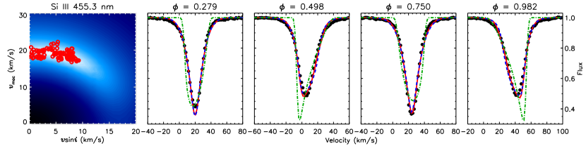
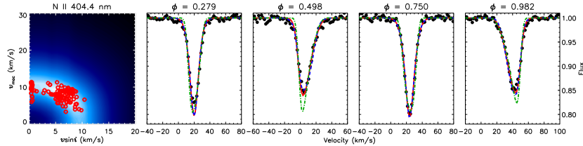
Figure 3: Line profile fitting to determine $v\sin i$ and $v_{\rm mac}$, using Si iii 455.3 nm (top) and N II 404.4 nm (bottom). Left: $\chi^{2}$ landscapes (high values are dark, low values are light, where the reduced $\chi^{2}$ goes from approximately 1 to $2\times 10^{5}$), corresponding to the weighted mean $\chi^{2}$ across all observations. The best-fit solutions for individual observations are indicated by open red circles. Right: line profile fits at pulsation phases close to the RV minima and maxima ($\phi=0.498,0.982$) and $RV=0$ km s^-1($\phi=0.279,0.750$). Observations are shown by black circles. The solid red line shows the best overall fit for each observation. The dashed blue line shows the best fit model with $v\sin{i}=0$ km s^-1. The dash-dotted green line indicates the best fit model with $v_{\rm mac}=0$ km s^-1. While the overall best-fit has a non-zero $v\sin i$ of a few km s^-1, excluding $v_{\rm mac}$ results in a noticeably worse fit, but excluding $v\sin i$ does not substantially worsen the fit. The weaker N ii line yields a lower $v_{\rm mac}$, but does not change the result that $v_{\rm mac}>v\sin{i}$, or that equivalently good fits can be achieved with or without $v\sin i$.

3.2 Frequency Analysis

We analyed the RVs using period04 (Lenz & Breger, 2005). Frequency spectra are shown in Fig. 1, where the top panels show the frequency spectra for the original dataset, and the panels below show frequency spectra after pre-whitening with the most significant frequencies from previous frequency spectra. A S/N threshold of 4 was adopted as the minimum S/N for significance (Breger et al., 1993; Kuschnig et al., 1997). The uncertainty in each frequency was determined using the formula from Bloomfield (1976), $\sigma_{\rm F}=\sqrt{6}\sigma_{\rm obs}/(\pi\sqrt{N_{\rm obs}}A\Delta T)$, where $\sigma_{\rm obs}$ is the mean uncertainty in the RV measurements, $N_{\rm obs}$ is the number of measurements, $A$ is the amplitude of the RV curve, and $\Delta T$ is the timespan of observations.

Period analysis of the CORALIE dataset (left panels in Fig. 1) yielded the same results as those reported by Saesen et al. (2006), with significant frequencies at $f_{\rm pul,COR}=4.7715297(5)~{}{\rm d}^{-1}$ with an amplitude of 16.6 km s^-1, and at the harmonics 2$f_{\rm pul,COR}$ and 3$f_{\rm pul,COR}$ with amplitudes of 0.6 km s^-1 and 0.3 km s^-1, respectively. After pre-whitening with these frequencies, no significant frequencies remain (bottom left panel of Fig. 1), and all peaks are at the 1$~{}{\rm d}^{-1}$ aliases of the spectral window. The same analysis of the ESPaDOnS data (middle panels in Fig. 1) finds maximum power at $f_{\rm pul,ESP}=4.7715007(4)~{}{\rm d}^{-1}$, and at 2$f_{\rm pul,ESP}$.

The combined dataset (right panels in Fig. 1) yields the strongest signal at $f_{\rm pul,Comb}=4.7715121(3)~{}{\rm d}^{-1}$, along with significant peaks at 2$f_{\rm pul,Comb}$ and 3$f_{\rm pul,Comb}$. In this case pre-whitening does not completely remove the peak corresponding to $f_{\rm pul,Comb}$. This could indicate that the pulsation frequency is not the same between the datasets. The difference in frequencies between the CORALIE and ESPaDOnS datasets, $2.9\times 10^{-5}~{}{\rm d^{-1}}$, is about 30 times larger than the formal uncertainties in either frequency. This difference corresponds to an increase in the pulsation period of 0.1 s, approximately compatible with the increase of $0.063\pm 0.009~{}{\rm s}$ expected from the constant period change of $+0.0037(5)~{}{\rm s}~{}{\rm yr}^{-1}$ reported by Jerzykiewicz (1999).

To explore this hypothesis, phases were calculated assuming a constant rate of period change $-0.02<\dot{P}<+0.02~{}{\rm s}~{}{\rm yr}^{-1}$, with $f_{0}=4.771529(7)~{}{\rm d}^{-1}$ taken as the frequency inferred from the CORALIE data acquired in 2000, and allowed to vary within the uncertainty in this frequency. The phases $\phi$ were calculated as

$$\phi=\frac{{\rm HJD}-(T_{0}+NP_{0}+0.5\dot{P}N^{2})}{P_{0}+N\dot{P}},$$ (1)

where $P_{0}$ is the initial period, and $N$ is the number of pulsation cycles elapsed between the observation and the reference epoch $T_{0}=2451591.42576$, defined as the time of the first RV maximum one cycle before the first observation in the dataset. The goodness-of-fit $\chi^{2}$ statistic was calculated for each combination of $P_{0}$ and $\dot{P}$ using a 3^rd-order least-squares sinusoidal fit in order to account for the pulsation frequency and its first two harmonics. The minimum $\chi^{2}$ solution was found for $P_{0}=0.2095763(1)~{}{\rm d}$ and $\dot{P}=+0.0096(5)~{}{\rm s}~{}{\rm yr}^{-1}$, where the uncertainties were determined from the range over which $\chi^{2}$ does not change appreciably. The RVs are shown phased with Eqn. 1 using these parameters in Fig. 2. The bottom panel of Fig. 2 shows the residual RVs after subtraction of the 3^rd-order sinusoidal fit. The standard deviation of the residuals is 0.48 km s^-1, an improvement over the standard deviation of 0.94 km s^-1 obtained using the constant period determined from the full dataset. The bottom right panel of Fig. 1 shows the frequency spectrum obtained for the residual RVs in Fig. 2: in contrast to the results obtained via pre-whitening using a constant pulsation frequency, all power at $f_{\rm pul}$ and its harmonics is removed, with no significant frequencies remainining.

3.3 Comparison to previous results

Our analysis of the CORALIE dataset recovers the same pulsation frequency as that found by the analysis performed by Saesen et al. (2006) of the same data. However, we find $\dot{P}$ to be almost 3 times larger than the rate found by Jerzykiewicz (1999). Whether this reflects an acceleration in the rate of period change will need to be explored in the future when larger datasets with a longer temporal baseline are available. Neilson & Ignace (2015) noted that $\xi^{1}$ CMa is one of the few $\beta$ Cep stars for which $\dot{P}$ is low enough to be consistent with stellar evolutionary models. The higher $\dot{P}$ suggested by our results brings $\xi^{1}$ CMa closer to the range observed for other $\beta$ Cep stars, which is to say, slightly above the $\dot{P}$ predicted by evolutionary models for a star of $\xi^{1}$ CMa’s luminosity.

4 Stellar Parameters

4.1 Line Broadening

The high S/N, high spectral resolution, and wide wavelength coverage of the ESPaDOnS data, combined with the sharp spectral lines of this star, present numerous opportunities for constraining the line broadening mechanisms. As with measurement of RVs, in order to minimize the impact of RV variation, Stokes $I$ spectra from individual sub-exposures were used rather than the spectra computed from the combined exposures. We selected two lines for analysis: the Si iii 455.3 nm line, which is sensitive to the pulsational properties of $\beta$ Cep stars (Aerts & De Cat, 2003), and for comparison N ii 404.4 nm, a weaker line with lower sensitivity to pulsation.

We applied a model incorporating the projected rotation velocity $v\sin i$, radial/tangential macroturbulence $v_{\rm mac}$, and assumed radial pulsations, performing a goodness-of-fit (GOF) test on a grid spanning 0–20 km s^-1 in $v\sin i$ and 0–30 km s^-1 in $v_{\rm mac}$, in 1 km s^-1 increments. The disk integration model is essentially as described by Petit & Wade (2012), with the exception of radial pulsations. Pulsations were modeled as a uniform velocity component normal to the photosphere, with the local line profiles in each surface area element shifted by the projected line-of-sight component of the pulsation velocity. A limb darkening coefficient of $\epsilon=0.36$ was used, obtained from the tables calculated by Díaz-Cordovés et al. (1995) for a star with $T_{\rm eff}$$=27$ kK and $\log{g}=3.75$. Local profiles were broadened with a thermal velocity component of 4 km s^-1 for Si iii, and 5.6 km s^-1 for N ii, and the disk integrated profile was convolved according to the resolving power of ESPaDOnS. Line strength was set by normalizing the EWs of the synthetic line profiles to match the EWs of the observed line profiles. In the course of this analysis we found a Baade-Wesselink projection factor of measured-to-disk-centre radial velocity of $p=1.45\pm 0.02$, which is consistent with determinations for other $\beta$ Cep variables (e.g., Nardetto et al. 2013).

Fig. 3 shows the resulting best-fit models. Taking the mean and standard deviation across all observations, both Si iii 455.3 nm and N ii 404.4 nm yield $v\sin{i}=5\pm 3$ km s^-1. The two lines give different values for $v_{\rm mac}$, however: 19$\pm$1 km s^-1 and 8$\pm$2 km s^-1, respectively. The much lower value of $v_{\rm mac}$ determined from N ii 404.4 nm may indicate that the extended wings of Si iii 455.3 nm, which require a higher value of $v_{\rm mac}$ to fit, are at least partly a consequence of pulsations.

As demonstrated in Fig. 3, there is essentially no difference in quality of fit between models with nonzero $v\sin i$ and $v_{\rm mac}$, and zero $v\sin i$; conversely, a much worse fit is obtained by setting $v_{\rm mac}=0$ km s^-1. For Si iii 455.3 nm, the $\chi^{2}$ of the model without $v_{\rm mac}$ is 13 times higher than the $\chi^{2}$ of the model without $v\sin i$, while the $\chi^{2}$ of the model without $v\sin i$ is only 1.4 times higher than the model with both turbulent and rotational broadening. The difference is not as great for N ii 404.4 nm, although the $\chi^{2}$ of the model with rotational broadening only is still higher than either the model with turbulent broadening only, or both rotational and turbulent broadening. Sundqvist et al. (2013) used magnetic O stars with rotational periods known to be extremely long (i.e. with $v\sin i$ $\sim 0$ km s^-1) and found that both the goodness-of-fit test and the Fourier transform methods severely over-estimate $v\sin i$ when $v_{\rm mac}>v\sin{i}$, as is the case for both of the lines we have examined. We conclude that the star’s line profiles are consistent with $v\sin i$ $=0$ km s^-1.

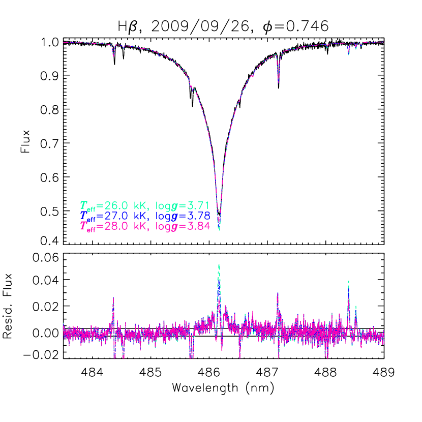
Figure 4: Surface gravity determination using H$\beta$. Top: model fits for $T_{\rm eff}$$=26,27$, and 28 kK (cyan, blue, and pink, respectively) to the observed profile (black). The observation nearest $\phi=0.75$ (where the RV$=0$ km s^-1) was used. Bottom: residuals. The horizontal lines indicate the mean flux uncertainty. As explored in § 7.1, there is emission near the line core; this is more prominent in H$\alpha$. This region was not included in the fit.

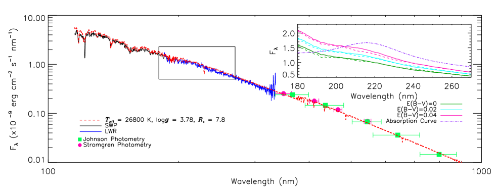
Figure 5: Low-resolution IUE spectroscopy (solid lines) with the SWP (black) and LWR (blue) cameras, and photometry (filled symbols) compared to a synthetic photospheric spectrum (red dashed line). No dereddening correction has been applied to the data. Inset: Comparison between synthetic spectra (dashed lines) and observed spectra (solid lines) deredded using three values of $E(B-V)$: 0 (green), 0.02 (cyan), and 0.04 (pink). Both the observed spectrum and the best-fit synthetic spectra have been smoothed with a boxcar algorithm. The dot-dashed (purple) line is the reddening curve in arbitrary units. Even mild dereddening produces a bulge in the vicinity of the 220 nm silicate absorption feature.

4.2 Surface Gravity

The surface gravity $\log{g}$ was determined by fitting tlusty BSTAR2006 synthetic spectra (Lanz & Hubeny, 2007) to the H$\beta$ and H$\gamma$ lines of the ESPaDOnS spectrum acquired at pulsation phases at which the RV was closest to the systemic velocity of 22.5 km s^-1 (i.e. at pulsation phases 0.25 or 0.75). As both of these lines are close to the edges of their respective orders, in order to avoid warping the line the orders were merged from un-normalized spectra, then normalized using a linear fit to nearby continuum regions. Five surface gravities were tested between $\log{g}=3.25$ and $\log{g}=4.25$, and a low-order polynomial was fit to the resulting $\chi^{2}$ in order to identify the lowest $\chi^{2}$ solution. Uncertainties were determined by fitting models with $T_{\rm eff}$ of 26, 27, and 28 kK, spanning the approximate range in the uncertainty in $T_{\rm eff}$ (see below). Fig. 4 shows the best-fit models, $\log{g}=3.78\pm 0.07$, compared to the observed H$\beta$ line. Fitting to H$\gamma$ yielded identical results.

4.3 Effective Temperature

The effective temperature $T_{\rm eff}$ was determined using photometry, spectrophotometry, and spectroscopy. Using the Strömgren $uvby\beta$ photometric indices obtained by Hauck & Mermilliod (1998), and the idl program uvbybeta.pro which implements the calibrations determined by Moon (1985), yields $T_{\rm eff}$$=26.2$ kK. Using the Johnson $UBVRIJHK$ photometry collected by Ducati (2002) and the colour-temperature calibration presented by Worthey & Lee (2011) yields $T_{\rm eff}$$=25\pm 3$ kK, where the uncertainty was determined from the range of $T_{\rm eff}$ across the $(U-B),(V-K),(B-V),(V-R)$, and $(J-K)$ colours.

The $T_{\rm eff}$ was measured using spectrophotometric data by fitting synthetic BSTAR2006 spectra to the IUE low-dispersion spectra, Johnson UBVRI photometry, and Strömgren $uvby\beta$ photometry. The Johnson photometry was converted into absolute flux units using the calibration provided by Bessell et al. (1998), and the Strömgren photometry converted using the calibration determined by Gray (1998). The synthetic spectra were scaled by $1/d^{2}$ and $4\pi R_{*}^{2}$, where the distance $d$ was fixed by the Hipparcos parallax and the stellar radius $R_{*}$ was left as a free parameter. The resulting fit is shown in Fig. 5. The best-fit model yields $T_{\rm eff}$$=26.8\pm 0.4$ kK and $R_{*}=7.8~{}R_{\odot}$. The uncertainty comes from the spread in $T_{\rm eff}$ over the range of $\log{g}=3.78\pm 0.07$, and for two values of $E(B-V)$, 0 and 0.02. Fluxes were dereddened using the idl routine fm_unred, which utilizes the Fitzpatrick & Massa (1990) extinction curve parameterization. As demonstrated by the inset in Fig. 5, there is a clear absence of interstellar silicate absorption near 220 nm. The de-reddened spectra in the inset in Fig. 5 assume the strength of the absorption bump is $c_{3}=2.1$, the minimum Galactic value (Clayton et al., 2003). Even with this low value of $c_{3}$, using $E(B-V)=0.04$ results in an increase of the flux near the silicate absorption bump which is not observed. Using the average Galactic value of $c_{3}=3.23$ instead would require that $E(B-V)$ be even lower.

4.4 Comparison to previous results

Previous measurements of $v\sin i$ have in general yielded somewhat higher, non-zero results than those obtained here ($15\pm 1.5$ km s^-1, Saesen et al. 2006; 9$\pm$2 km s^-1, Lefever et al. 2010; 14$\pm$5 km s^-1, Aerts et al. 2014). Saesen et al. did not include $v_{\rm mac}$ in their profile fit, but did include pulsation and thermal broadening; Lefever et al. did not consider pulsations; and Aerts et al. included $v_{\rm mac}$, but neither pulsation velocity nor thermal broadening. Our inclusion of thermal, macroturbulent, pulsational, and rotational velocity fields likely explains why our best-fit value of $v\sin i$, $5\pm 3$ km s^-1, is somewhat lower than the values found previously, since all four sources of line broadening are of a similar magnitude in this star.

Stellar parameters for $\xi^{1}$ CMa have been determined numerous times using a variety of different spectral modelling methodologies, e.g., DETAIL/SURFACE (Morel et al., 2008), FASTWIND (Lefever et al., 2010), and PoWR (Oskinova et al., 2011). Niemczura & Daszyńska-Daszkiewicz (2005) employed an algorithmic method to simultaneously determine reddening, $T_{\rm eff}$, metallicities, and surface gravities for $\beta$ Cep stars observed with IUE, and for $\xi^{1}$ CMa found $T_{\rm eff}$ $=24\pm 1$ kK, $\log{g}=3.89$, and $E(B-V)<0.01$, i.e. their analysis favoured a cooler, slightly less evolved star, but with the same very low level of reddening. Niemczura & Daszyńska-Daszkiewicz derived $\log{g}$ from photometric calibrations, rather than line profile fitting, which likely explains the different values of $\log{g}$. Morel et al. (2008) found $T_{\rm eff}$ $=27.5$ kK and $\log{g}=3.75$, Lefever et al. (2010) derived $T_{\rm eff}$ $=27\pm 1$ kK and $\log{g}=3.80\pm 0.15$, and Oskinova et al. (2011) found $T_{\rm eff}$ $=27.5\pm 0.5$ kK: all are in agreement with the results found here. The slightly higher $T_{\rm eff}$ found in these works is likely a consequence of the higher value of reddening which, as is shown in § 4.3 and Fig. 5, is not consistent with the absence of silicate absorption. While reddening has an effect on the spectrophotometric method applied in § 4.3, we obtained essentially identical results using line strength ratios and ionization balances below in § 4.5, which should not be affected by reddening.

4.5 Effective Temperature Variation

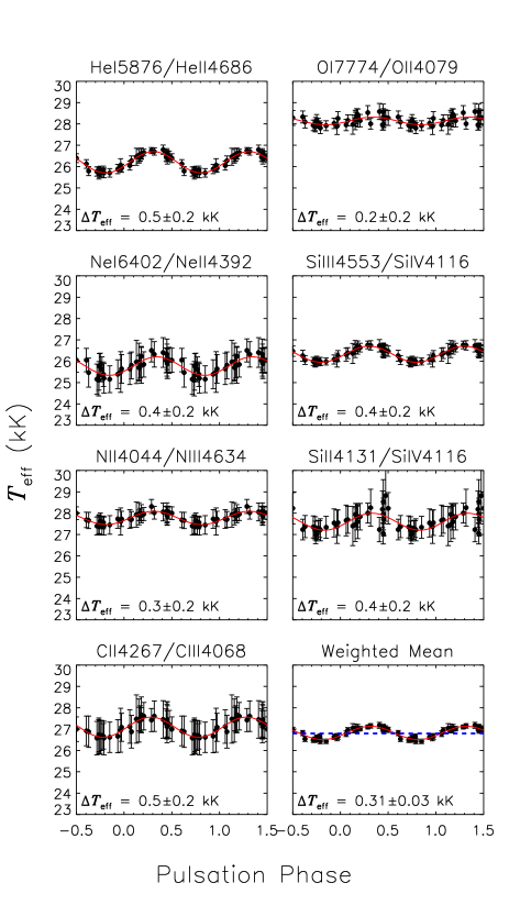
Figure 6: $T_{\rm eff}$ determined from EW ratios of various ion pairs as a function of pulsation phase. While the mean $T_{\rm eff}$ differs by $\sim$2 kK between different ion pairs, a coherent and identical modulation with the pulsation period is seen in all cases. The semi-amplitude of the $T_{\rm eff}$ variation, as determined from the least-squares sinusoidal fit to the data, is given at the bottom of each panel. The bottom right panel shows the weighted mean $T_{\rm eff}$ across all ion pairs, with the dashed blue line indicating the $T_{\rm eff}$ determined from SED fitting (Fig. 5).

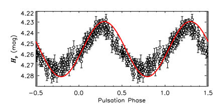
Figure 7: Predicted variation in visual magnitude (red line) as determined from the variation in $R_{*}$ from RVs (Fig. 2) and in $T_{\rm eff}$ from EW ratios (Fig. 6) as compared to the Hipparcos photometry (black circles). Pulsation phases were calculated using eqn. 1.

The photospheric temperature of a $\beta$ Cephei star is variable, a property which can be explored both photometrically and spectroscopically. The only public two-colour photometry for $\xi^{1}$ CMa are the Tycho $BV_{\rm T}$ observations. While pulsational modulation is visible in both passbands, the precision of the data is not sufficient to detect a coherent signal in the colours. This is not surprising, as $B-V$ colours are poorly suited to determining $T_{\rm eff}$ for such hot stars. We therefore attempted to constrain the $T_{\rm eff}$ change via the ionization balances of various spectral lines, under the assumption that all equivalent width (EW) changes are due to temperature variation.

We first measured EWs from the ESPaDOnS observations, and from appropriate synthetic spectra obtained from the tlusty BSTAR2006 library (Lanz & Hubeny, 2007). We used the ESPaDOnS Stokes $I$ spectra obtained from the combined sub-exposures, in order to maximize the S/N. The following spectral lines were used: He i 587.6 nm, He ii 468.6 nm, C ii 426.7 nm, C iii 406.8 nm, N ii 404.4 nm, N iii 463.4 nm, O i 777.4 nm, O ii 407.9 nm, Ne i 640.2 nm, Ne ii 439.2 nm, Si ii 413.1 nm, Si iii 455.3 nm, and Si iv 411.6 nm. Since the EW can depend on $\log{g}$ as well as $T_{\rm eff}$, the model EW ratios were linearly interpolated to $\log{g}=3.78$ between the results for $\log{g}=3.75$ and $\log{g}=4.0$. We then determined $T_{\rm eff}$ by interpolating through the resulting grid to the EW ratios measured from the observed spectra. The results are illustrated in Fig. 6. While there is a considerable spread in values, from approximately 25 to 28 kK, the mean value of 26.8 kK agrees well with the spectrophotometric determination. A coherent variation with the pulsation period is seen for all ion strength ratios. Individual atomic species yield variations with semi-amplitudes up to $\Delta T_{\rm eff}=\pm 500$ K. Taking the weighted mean across the effective temperatures from all ion strength ratios at each phase yields a variation of $\Delta T_{\rm eff}=\pm 310\pm 30$ K. If the zero-point of each $T_{\rm eff}$ variation is first subtracted, the resulting mean $T_{\rm eff}$ semi-amplitude is $330\pm 30$ K, slightly larger but overlapping within the uncertainty.

To check the validity of the temperature variation, we used it to model the Hipparcos light curve, as demonstrated in Fig. 7. With the uncertainty in the pulsation period and rate of period change determined in § 3, the accumulated uncertainty in pulsation phase for the Hipparcos photometry is between 0.009 and 0.012 cycles. We began by determining the mean radius $R_{*}$ from the mean $T_{\rm eff}$ and the luminosity $\log{L}$. $\log{L}$ was obtained from the Hipparcos parallax distance $d=424\pm 35$ pc, the apparent $V$ magnitude 4.06, and the bolometric correction $BC=-2.61\pm 0.09$ mag obtained by linear interpolation through the theoretical BSTAR2006 grid according to $T_{\rm eff}$ and $\log{g}$ (Lanz & Hubeny, 2007). The absolute $V$ magnitude $m_{V}=V-A_{V}-\mu=-3.86\pm 0.18$ mag, where $\mu=5\log{d}-5=8.13\pm 0.18$ mag is the distance modulus and $A_{V}=E(B-V)/3.1<0.06$ mag is the extinction. The bolometric magnitude is then $M_{\rm bol}=m_{V}+BC=-6.47\pm 0.27$ mag, yielding $\log{(L/L_{\odot})}=(M_{\rm bol,\odot}-M_{\rm bol})/2.5=4.49\pm 0.11$ where $M_{\rm bol,\odot}=4.74$ mag. This yields $R_{*}=\sqrt{(L/L_{\odot})/(T_{\rm eff}/T_{\rm eff,\odot})^{4}}=7.9\pm 0.6~{}R_{\odot}$, where $T_{\rm eff,\odot}=5.78$ kK. This radius agrees well with the value found via spectrophotometric modelling, $R_{*}=7.8~{}R_{\odot}$, in which the radius was left as a free parameter (Fig. 5).

Integrating the radial velocity curve (Fig. 2) in order to obtain the absolute change in radius, and assuming radial pulsation, yields a relatively small change in radius of $\pm 6.58\times 10^{4}$ km, corresponding to between 1.0 and 1.5% of the stellar radius. The radius variation was then combined with the $T_{\rm eff}$ variation from Fig. 6 to obtain $\log{L}$ and the $BC$ at each phase. The apparent $V$ magnitude was then obtained by reversing the calculations in the previous paragraph. The solid red line in Fig. 7 shows the resulting model light curve compared to the Hipparcos photometry, where we made the assumption that $V$ and $H_{\rm p}$ are approximately equivalent. The larger 500 K $T_{\rm eff}$ semi-amplitude measured from individual pairs of ions is not consistent with the light curve, yielding a photometric variation larger than observed, with a semi-amplitude of 0.037 mag as compared to the observed semi-amplitude of $\sim$0.021 mag. The apparent phase offset of $\sim$0.05 cycles between the predicted and observed photometric extrema may suggest that $\dot{P}$ may not in fact be constant; alternatively, there may simply be too few measurements to constrain the $T_{\rm eff}$ variation well enough to obtain a close fit to the photometric data, as the latter is clearly not a perfect sinusoid.

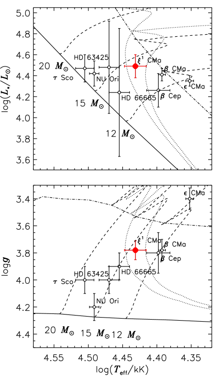
Figure 8: $\xi^{1}$ CMa’s position on the HRD (top) and on the $T_{\rm eff}$-$\log{g}$ diagram (bottom), relative to other magnetic stars with similar stellar parameters. The solid line indicates the Zero-Age Main Sequence (ZAMS), and the dot-dashed line the Terminal Age Main Sequence (TAMS). Dashed lines show evolutionary tracks from the (rotating, non-magnetic) models by Ekström et al. (2012), and dotted lines isochrones from the same models for $\log{(t/{\rm yr})}=7.0$ (left) and 7.1 (right). The star’s fundamental parameters indicate $M_{*}=14.2\pm 0.4M_{\odot}$ and $t=11\pm 0.7$ Myr. $\xi^{1}$ CMa is the most evolved magnetic B-type star above about 12 $M_{\odot}$.

4.6 Mass and Age

Fig. 8 shows $\xi^{1}$ CMa’s position on the Hertzsprung-Russell diagram (HRD) (top) and the $T_{\rm eff}$-$\log{g}$ diagram (bottom), where the mean $T_{\rm eff}$ was used. Comparison to the evolutionary models calculated by Ekström et al. (2012) (which assume an initial rotational velocity of 40% of the critical velocity) indicates that the stellar mass $M_{*}=14.2\pm 0.4~{}M_{\odot}$, and that the absolute stellar age is $t=11\pm 0.7$ Myr. The Ekström et al. (2012) models do not include the effects of magnetic fields, however, grids of self-consistent evolutionary models including these effects in a realistic fashion are not yet available.

The positions of the star on the two diagrams are mutually consistent. The other known magnetic B-type stars with similar stellar parameters are also shown in Fig. 8. The stellar parameters of the majority of the other stars were obtained from the catalogue of magnetic hot stars published by Petit et al. (2013) and references therein; those of $\beta$ CMa and $\epsilon$ CMa were obtained from Fossati et al. (2015a). $\xi^{1}$ CMa is one of the most evolved stars in the ensemble, and is the most evolved star with a mass above about 12 $M_{\odot}$. Its position on the $T_{\rm eff}$-$\log{g}$ diagram indicates it may be a more evolved analogue of NU Ori, HD 63425, and HD 66665.

Table 1: Observational and physical properties. The third column gives the reference, where numerical references indicate the section within this paper where the parameter is determined.

$v_{\rm sys}$ (km s-1)	22.5$\pm$1	3
$v\sin i$ (km s-1)	$\leq 8$	4.1
$v_{\rm mac}$ (km s-1)	8$\pm$2	4.1
Sp. Type	B0.5 IV	Hubrig et al. (2006)
$V$ (mag)	4.3	Ducati (2002)
$\pi$ (mas)	2.36$\pm$0.2	van Leeuwen (2007)
$d$ (pc)	424$\pm$35	van Leeuwen (2007)
$BC$ (mag)	-2.61$\pm$0.09	4.5
$A_{\rm V}$ (mag)	$<0.06$	4.5
$m_{\rm V}$ (mag)	-3.86$\pm$0.18	4.5
$M_{\rm bol}$ (mag)	-6.47$\pm$0.27	4.5
$\log{(L/L_{\odot})}$	4.49$\pm$0.11	4.5
$T_{\rm eff}$ (kK)	27$\pm$1	4.3
$\log{g}$	3.78$\pm$0.07	4.2
$R_{*}~{}(R_{\odot})$	7.9$\pm$0.6	4.3
$M_{*}~{}(M_{\odot})$	14.2$\pm$0.4	4.6
Age (Myr)	11.1$\pm$0.7	4.6
$\tau_{\rm MS}$	0.77$\pm$0.04	4.6
$R_{*}/R_{\rm ZAMS}$	1.8$\pm$0.1	4.6

As an additional check on the stellar mass and radius, we utilized the pulsation period and the relation $P_{\rm fun}=\frac{Q}{\sqrt{\rho}}$, where $P_{\rm fun}$ is the fundamental pulsation period, $\rho$ is the mean density, and $Q$ is the pulsation constant. With $M_{*}=14.2\pm 0.4~{}M_{\odot}$, $R_{*}=7.9\pm 0.6~{}R_{\odot}$, and the theoretical value $Q=0.035$ (Davey, 1973; Stothers, 1976), this yields $P_{\rm fun}=0.18\pm 0.02$ d, very close to the true pulsation period $P\sim 0.21$ d. If the actual pulsation period is used to calculate $Q$, we obtain $Q=P_{\rm fun}\sqrt{\rho}=0.041\pm 0.003$.

5 Binarity

5.1 Interferometry

Fourtune-Ravard et al. (2011) reported that $\xi^{1}$ CMa hosts weak H$\alpha$ emission, which is atypical for a star of $\xi^{1}$ CMa’s stellar properties. There are two possibilities to explain this: first, that it originates in a stellar magnetosphere, and second, that it originates in the decretion disk of a heretofore undetected Be companion star. It seems reasonable to expect that $\xi^{1}$ CMa has a binary companion, as the binary fraction is $\sim$65% for B0 stars (Chini et al., 2012). Furthermore, early claims that the H$\alpha$ emission of $\beta$ Cep, a similar magnetic early-B type pulsator, originated in its magnetosphere (Donati et al., 2001), proved unfounded following the detection of a Be companion star by Schnerr et al. (2006).

The peak H$\alpha$ emission has a maximum strength of 28% of the continuum (see § 7.1). Be star emission lines can range up to $\sim 10\times$ of the continuum, although the emission is typically much less than this. We therefore expect that the putative companion must have a luminosity of $\geq 2.8\%$ of that of $\xi^{1}$ CMa, yielding $\log{(L/L_{\odot})}\geq 2.9$ or $V<7.6$. Assuming the pair to be coeval, and therefore locating the star on the same isochrone as $\xi^{1}$ CMa, the companion’s mass should be near $5~{}M_{\odot}$, compatible with a classical Be star.

$\xi^{1}$ CMa is listed in the Washington Double Star Catalogue as possessing a binary companion (Mason et al., 2001). However, the reported companion is both too dim to account for the H$\alpha$ emission ($V=14$) and too far away, located approximately 28” from the primary, i.e. well outside the 1.6” ESPaDOnS aperture.

We acquired H and K low-resolution VLTI-AMBER data, together with VLTI-PIONIER data, in order to search for the presence of a binary star. The squared visibilities $V^{2}$ and closure phases $\phi_{\rm C}$ of these data are shown as functions of spatial frequency in Fig. 9. Both the AMBER K band and PIONIER $V^{2}$ measurements are entirely flat, compatible with a single unresolved source. There is furthermore no signal in the PIONIER $\phi_{\rm C}$ measurements, which are more precise than those available from AMBER.

We analyzed the data using the standard litpro package (Tallon-Bosc et al., 2008), fitting a two-point model, with one point fixed in the centre of the map and the (x,y) coordinates of the second free to move. The overall upper limit on the flux of a secondary component is 1.7% of the primary star’s flux. In order to constrain the maximum flux of a binary companion at different distances from the primary, we repeated the two-point model fit in successively wider boxes (as the current version of litpro does not support polar coordinates, a Cartesian approximation to annuli was used). As these flux ratios are in the $H$ and $K$ bands, but our estimated minimum flux ratio is in the $V$ band, we used synthetic tlusty SEDs (Lanz & Hubeny, 2007) to convert the $H$ and $K$ band flux ratios to $V$ band flux ratios. In this step we assumed that the secondary’s $T_{\rm eff}$ is near 20 kK, appropriate to a 5-6 $M_{\odot}$ star near the main sequence. A companion of the required brightness is ruled out beyond $\sim 40$ AU.

Close binaries containing magnetic, hot stars are extremely rare, with $<2$% of close binary systems containing a magnetic companion earlier than F0 (Alecian et al., 2015). This does not mean that a close companion can be ruled out a priori. Such a companion may be detectable via radial velocities. As found in § 3, the RV curve of $\xi^{1}$ CMa is extremely stable, with a standard deviation of the residual RVs of $\sim$0.5 km s^-1. To determine if a Be companion should have been detected, we computed radial velocities across a grid of models with secondary masses $1~{}M_{\odot}<M_{\rm S}<10~{}M_{\odot}$, semi-major axes $0.05~{}{\rm AU}<a<500~{}{\rm AU}$, eccentricities $0<e<0.9$, and inclinations of the orbital axis from the line of sight $1^{\circ}<i<90^{\circ}$. We then phased the JDs of the observations with the orbital periods $P_{\rm orb}$, using a single zero-point if $P_{\rm orb}$ was less than the time-span of the observations and multiple, evenly-spaced zero-points if $P_{\rm orb}$ was greater than this span. We then calculated the expected RV of the primary at each orbital phase, and compared the standard deviation $\sigma_{\rm orb}$ of these RVs with the observed standard deviation $\sigma_{\rm obs}$ (RV amplitudes were not used as, for orbits with periods longer than the timespan of observations, the full RV variation would not have been sampled). A given orbit was considered detectable if $\sigma_{\rm orb}>3\sigma_{\rm obs}$. Numerical experiments with synthetic RV curves including gaussian noise with a standard deviation of 0.5 km s^-1 indicate that this criterion is likely conservative: with 624 RV measurements, input periods can generally be recovered even when the semi-amplitude of the RV curve is similar to the noise level.

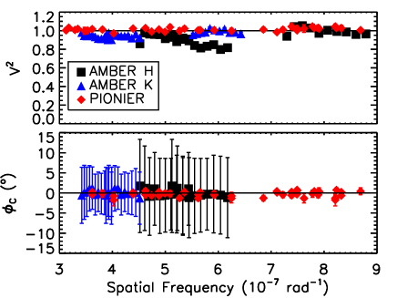
Figure 9: Low-resolution VLTI-AMBER H and K data and VLTI-PIONIER data, showing squared visibilities (top) and closure phases (bottom).

Each orbit was assigned a probability $P(i)$ assuming a random distribution of $i$ over $4\pi$ steradians (i.e., $P(i)=1-\cos{i}$), and a flat probability distribution for $M_{\rm S}$, $e$, and $a$. From this we obtained the 1, 2, and 3$\sigma$ upper limits on a companion’s mass as a function of $a$. This mass upper limit was then transformed into a $V$ magnitude lower limit by interpolating along the 10 Myr isochrone in Fig. 8. Within the 40 AU inner boundary of the interferometric constraints, a binary companion of sufficient brightness to host the H$\alpha$ emission can be ruled out entirely at 1$\sigma$ confidence, and almost entirely at 2$\sigma$.

We have proceeded under the very conservative assumption of a Be star with H$\alpha$ emission of 10$\times$ its continuum level, however the majority of Be stars have emission of at most a few times the continuum, and many have much less than this. Thus, the upper limits on companion mass and brightness determined above rule out all but the most exceptional of classical Be stars as a possible origin for the H$\alpha$ emission. We conclude that there is unlikely to be an undetected binary classical Be companion star that is sufficiently bright to be the source of the star’s H$\alpha$ emission.

5.2 Spectro-interferometry

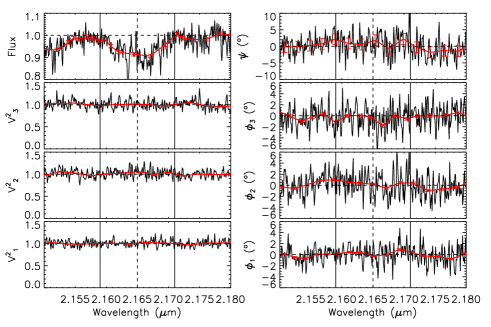
Figure 10: High-resolution VLTI/AMBER data showing (clockwise from top left), flux, closure phase $\psi$, differential phases $\phi_{i}$, and squared visibilities $V^{2}_{i}$. Black shows the raw data. Red lines show data binned to 20% of the mean error bar in the raw data. Vertical dashed lines indicate the central wavelength of the Br$\gamma$ line, solid vertical lines denote the extent of the line.

The formation of the line emission around the $\beta$ Cep star itself is supported by the absence of any spectrointerferometric signal across the Br$\gamma$ line. Such observations were taken with AMBER, and no signature in phase was detected on the level of 2^∘ (Fig. 10). This means that the photometric position as a function of wavelength remained stable on the level of 60 $\mu$as (Lachaume, 2003; Štefl et al., 2009). An emission component of about 30% of the strength of the continuum (Br$\gamma$ emission typically being comparable in strength to that of H$\alpha$ in Be stars) must therefore have its photocenter within 60 $\mu$as from the photocenter of the nearby continuum, as otherwise it would have produced a detectable offset of the phase signal. This not only excludes a general offset from the central star, i.e. formation around a companion, but also an extended orbiting structure, in which the blue emission would be formed at an offset opposite to the red emission.

6 Magnetic Field

6.1 Least Squares Deconvolution

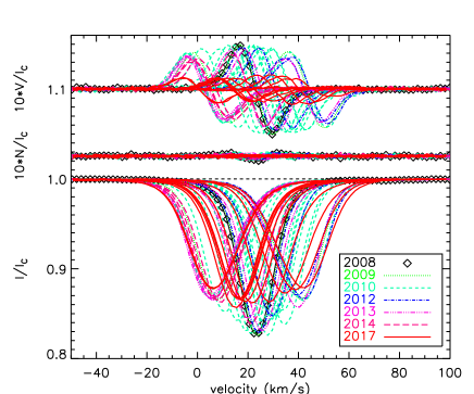
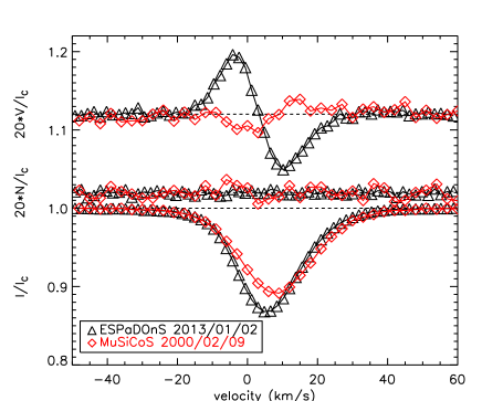
Figure 11: Top: ESPaDOnS LSD profiles: Stokes $I$ (bottom), $N$ (middle), Stokes $V$ (top). Bottom: ESPaDOnS (black triangles) and MuSiCoS (red diamonds) LSD profiles, extracted with identical line masks, from observations acquired at similar pulsation phases ($\sim$0.44). The broader and shallower MuSiCoS profile is a consequence of the much longer exposure times of the MuSiCoS observations, the instrument’s lower spectral resolution, and the intrinsic variability of the star. While the MuSiCoS LSD profile is obviously noisier, the Stokes $V$ signature is clearly of the opposite polarity of the ESPaDOnS observation.

While $\xi^{1}$ CMa’s sharp spectral lines and the high S/N of the ESPaDOnS observations mean that Zeeman signatures are visible in numerous individual spectral lines, in order to maximize the S/N we employed the usual Least Squares Deconvolution (LSD; Donati et al. 1997) multiline analysis procedure. In particular we utilized the ‘improved LSD’ (iLSD) package described by Kochukhov et al. (2010). iLSD enables LSD profiles to be extracted with two complementary line masks, improving the reproduction of Stokes $I$ and $V$ obtained from masks limited to a select number of lines.

We used a line mask obtained from the Vienna Atomic Line Database (VALD3; Piskunov et al. 1995; Ryabchikova et al. 1997; Kupka et al. 1999, 2000) for a solar metallicity star with $T_{\rm eff}$ $=27$ kK. While magnetic early-type stars are often chemically peculiar, $\xi^{1}$ CMa is of essentially solar composition (Niemczura & Daszyńska-Daszkiewicz, 2005), albeit with a mild N enhancement (Morel et al., 2008), thus a solar metallicity mask is appropriate. The mask was cleaned and tweaked as per the usual procedure, described in detail by Grunhut (2012), such that only metallic lines unblended with H, He, interstellar, or telluric lines remained, with the strengths of the remaining lines adjusted to match as closely as possible the observed line depths. Of the initial 578 lines in the mask, 338 remained following the cleaning/tweaking procedure. The resulting LSD profiles are shown in Fig. 11 (top panel). Note that, due to intrinsic line profile variability and the longer subexposure times used for the 2017 data, the line profiles of the most recent data are slightly broader than the data acquired previously.

In order to directly compare MuSiCoS and ESPaDOnS results, a second line mask was employed with all lines outside of the MuSiCoS spectral range removed, leaving 139 lines. The bottom panel of Fig. 11 shows a comparison between the highest S/N MuSiCoS LSD profile and the ESPaDOnS LSD profile with the closest pulsation phase (0.4377 vs. 0.4425). The Stokes $I$ profiles from the 2 instruments agree well, considering both the lower spectral resolution and the much longer exposure times of MuSiCoS (corresponding to $\sim$15% of a pulsation period, as compared to $\sim$2.3% of a pulsation period for ESPaDOnS). The key point of interest is in Stokes $V$, which is clearly negative in the MuSiCoS LSD profile, but positive in all ESPaDOnS LSD profiles. The second MuSiCoS observation also yields a negative Stokes $V$ profile. The reliability of these MuSiCoS observations is evaluated in detail in Appendix A.

False Alarm Probabilities (FAPs) were calculated inside and outside of the line profile, and classified as Definite Detections (DDs), Marginal Detections (MDs), or Non-Detections (NDs) according the methodology and criteria described by Donati et al. (1992, 1997). Detection flags for Stokes $V$ and diagnostic null $N$ are given in Table B4. All MuSiCoS observations are formal non-detections. All ESPaDOnS observations are DDs (with the exception of the two discarded measurements from 2017/02/11, both of which yielded NDs due to their low S/N). However, in numerous ESPaDOnS observations, $N$ also yields a DD. This phenomenon is considered in greater detail in § 9.1.

6.2 Longitudinal Magnetic Field

The longitudinal magnetic field $\langle B_{z}\rangle$ was measured from the LSD profiles by taking the first-order moment of the Stokes $V$ profile normalized by the equivalent width of Stokes $I$ (Mathys, 1989). The same measurement using $N$ yields the null measurement $\langle N_{z}\rangle$, which should be consistent with 0 G. In order to ensure a homogeneous analysis, the LSD profiles were first shifted by their measured RVs to zero velocity, and an identical integration range of $\pm 30$ km s^-1 around line centre employed. $\langle B_{z}\rangle$ and $\langle N_{z}\rangle$ measurements are reported in Table B4. As expected from the LSD profiles, $\langle B_{z}\rangle$$<0$ for both MuSiCoS measurements, while $\langle B_{z}\rangle$$>0$ for all ESPaDOnS measurements. The ESPaDOnS data are of much higher quality, with a median $\sigma_{B}=6$ G, as compared to 57 G for the MuSiCoS data. In contrast to the FAPs, in which many ESPaDOnS $N$ profiles yield definite detections, $\langle N_{z}\rangle$$/\sigma_{N}$ is typically very low, with a maximum of 2.4 and a median of 0.6, i.e. statistically identical to zero.

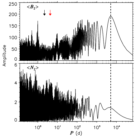
Figure 12: Periodograms for ESPaDOnS $\langle B_{z}\rangle$ (top) and $\langle N_{z}\rangle$ (bottom). Many of the peaks in the $\langle B_{z}\rangle$ periodogram also appear in the $\langle N_{z}\rangle$ periodogram, with the exception of the maximum amplitude peak at $\sim$5100 d (vertical dashed line). The period determined from FORS1/2 data by Hubrig et al. (2011) is indicated by the black arrow; the period determined by Fourtune-Ravard et al. (2011) from an earlier, smaller ESPaDOnS dataset is indicated by the red arrow. There is very little amplitude at either period.

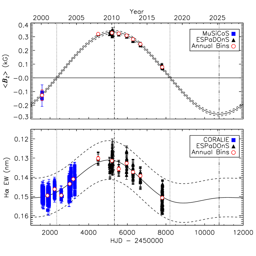
Figure 13: Top: $\langle B_{z}\rangle$ vs. time. The solid curve shows the least-squares sinusoidal fit to the annual mean measurements using a 30-year period, and the dashed curves indicate the $1\sigma$ uncertainty in the amplitude and mean value of the fit. The horizontal solid line shows $\langle B_{z}\rangle$ $=0$. Vertical lines indicate the times at which $\langle B_{z}\rangle$ $=0$ (dotted), $\langle B_{z}\rangle$$=$$\langle B_{z}\rangle$_max (dot-dashed), and $\langle B_{z}\rangle$$=$$\langle B_{z}\rangle$_min (dot-dot-dashed). Bottom: H$\alpha$ EWs. Curves show the least-squares $2^{nd}$-order sinusoidal fit to the annual means, which is performed independently of the fit to $\langle B_{z}\rangle$. Note that maximum emission corresponds to $\langle B_{z}\rangle$_max, and minimum emission corresponds to $\langle B_{z}\rangle$ $=0$. Also note that the fit predicts a second, weaker emission peak corresponding to $\langle B_{z}\rangle$_min.

Because $\langle B_{z}\rangle$ is expected to be modulated by stellar rotation, it can be used to determine the rotation period. The periodograms for $\langle B_{z}\rangle$ and $\langle N_{z}\rangle$ are shown in Fig. 12, where the latter shows the variation arising from noise. There are numerous peaks at periods of a few tens to a few hundreds of days which appear in both the $\langle N_{z}\rangle$ and the $\langle B_{z}\rangle$ periodograms. Phasing $\langle B_{z}\rangle$ with the periods corresponding to these peaks does not produce a coherent variation (e.g., phasing the data with the highest peak in this range, at 177 d, and fitting a first-order sinusoid, yields a reduced $\chi^{2}$ of 1162). The strongest peak in the $\langle B_{z}\rangle$ periodogram is at $5100\pm 300$ d. This peak does not appear in the $\langle N_{z}\rangle$ periodogram. This is similar to the timespan of the ESPaDOnS dataset, and so the formal uncertainty is certainly under-estimated, with the 5100 d period representing a lower limit. However, the S/N of this peak is 26, above the threshold for statistical significance, indicating that the long-term variation is probably real.

Fig. 13 shows the $\langle B_{z}\rangle$ measurements, both individual (filled symbols) and in annual bins (open circles), as a function of time. There is an obvious long-term modulation, with $\langle B_{z}\rangle$ steadily declining from a peak of $\sim$330 G in 2010 (HJD 2455200) to value of $\sim$80 G in 2017 (HJD 2457800). The annual mean $\langle B_{z}\rangle$ measurements are provided in Table 2.

Table 2: Annual weighted mean $\langle B_{z}\rangle$ measurements and H$\alpha$ EWs. Months/years and HJDs correspond to the mean of the cluster of observations within each bin.

Month/Year	HJD -	$\langle B_{z}\rangle$	H$\alpha$ EW
	2450000	(G)	(nm)
02/2000	2451585	-127$\pm$40	–
10/2000	2451822	–	0.1492$\pm$0.0002
11/2001	2452234	–	0.1462$\pm$0.0003
11/2002	2452580	–	0.1494$\pm$0.0007
12/2003	2452989	–	0.1440$\pm$0.0003
05/2004	2453156	–	0.1413$\pm$0.0002
01/2008	2454489	314$\pm$6	0.130$\pm$0.001
01/2010	2455203	328$\pm$2	0.1314$\pm$0.0004
12/2010	2455556	318$\pm$6	0.136$\pm$0.001
02/2012	2455965	305$\pm$3	0.1327$\pm$0.0007
01/2013	2456294	281$\pm$3	0.1373$\pm$0.0006
01/2014	2456674	253$\pm$5	0.1392$\pm$0.0008
02/2017	2457797	78$\pm$2	0.1507$\pm$0.0003

The MuSiCoS observations, both of which are of negative polarity, indicate (in combination with the ESPaDOnS data) that the rotational period must be longer than 5100 d. The time difference between the MuSiCoS measurements and the maximum $\langle B_{z}\rangle$ ESPaDOnS observations is $\sim$3600 d. If these two epochs sample the $\langle B_{z}\rangle$ curve at its positive and negative extrema, then the rotational period must be at least 7200 d ($\sim$20 years), or a half-integer multiple if there is more than one cycle between the observed extrema. The curvature of the ESPaDOnS $\langle B_{z}\rangle$ suggests that $\langle B_{z}\rangle$_max occurred at $\sim$HJD 2455200, however as it cannot be ruled out that $\langle B_{z}\rangle$${}_{\rm min}<-127\pm 40$ G, it is possible that $P_{\rm rot}>7200$ d. Indeed, a longer period seems likely: phasing $\langle B_{z}\rangle$ with a 20-year period, and fitting a least-squares $1^{st}$-order sinusoid (as expected for a dipolar magnetic field), produces a very poor fit as compared to longer periods. In Fig. 13, the illustrative sinusoudal fit was performed using a 30-year period, which achieves a reasonable fit to the data (the reduced $\chi^{2}$ is 2.6). Note that with this fit the MuSiCoS data do not define $\langle B_{z}\rangle$_min. Longer periods can also be accommodated, however at the expense of $|\langle B_{z}\rangle_{\rm min}|>|\langle B_{z}\rangle_{\rm max}|$. We thus adopt $P_{\rm rot}=30$ yr as the most conservative option allowed by the data.

6.3 Comparison to previous results

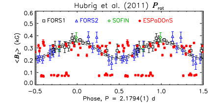
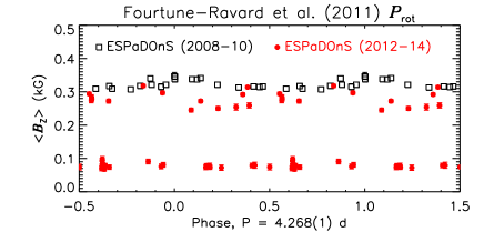
Figure 14: Top: ESPaDOnS, FORS1, FORS2, and SOFIN $\langle B_{z}\rangle$ measurements phased with the rotational period poposed by Hubrig et al. (2011). Bottom: ESPaDOnS $\langle B_{z}\rangle$ measurements phased with the rotational period proposed by Fourtune-Ravard et al. (2011). Neither of the previously proposed periods provides an acceptable phasing of the data.

There are two competing claims for rotational periods in the literature. The first, based on spectropolarimetry collected with FORS1, FORS2, and SOFIN, is approximately 2.18 d (Hubrig et al., 2011). The second period, based on a preliminary analysis of an earlier, smaller ESPaDOnS dataset, is $\sim 4.27$ d (Fourtune-Ravard et al., 2011). Period analysis of the ESPaDOnS measurements using Lomb-Scargle statistics rules out both of these periods. The rotational periods provided by Hubrig et al. (2011) and Fourtune-Ravard et al. (2011) are respectively indicated with black and red arrows in the top panel of Fig. 12. There is no significant power in the periodogram at either period. The peak corresponding to the Fourtune-Ravard et al. (2011) period appears in both the $\langle B_{z}\rangle$ and $\langle N_{z}\rangle$ periodograms, suggesting it to be a consequence of noise. Phasing the data with the periods given by Hubrig et al. (2011) or Fourtune-Ravard et al. (2011) does not produce a coherent variation, as is demonstrated in Fig. 14. It impossible for a period on the order of days to account for the systematic decline of $\sim$200 G between the earliest data and the most recent data. We also note that the ESPaDOnS dataset presented here includes two epochs with superior time-sampling to that of the FORS1/2 datasets: 14 observations over 10 d in 2010, and 20 observations over 38 d in 2017, as compared to 13 FORS1 observations over 1075 d and 11 FORS2 observations over 60 d. The ESPaDOnS dataset thus enables a much better probe than the FORS1/2 dataset of short-term as well as long-term variability.

All FORS1/2 and SOFIN measurements are of positive polarity (Hubrig et al., 2006, 2011; Fossati et al., 2015b), in agreement with ESPaDOnS data. Furthermore, the magnitude, $\sim$300 G, is similar. The two SOFIN measurements also agree well with the ESPaDOnS data. The much shorter 2.18 d period determined by Hubrig et al. (2011) is due to an apparent $\langle B_{z}\rangle$ variation with a semi-amplitude that is significant at 1.8$\sigma$ in comparison with the median uncertainties in these measurements. Bagnulo et al. (2012) showed that systematic sources of uncertainty such as instrumental flextures must be taken into account in the evaluation of $\langle B_{z}\rangle$ uncertainties from FORS1 data, that the uncertainties in FORS1 $\langle B_{z}\rangle$ measurements should thus be about 50% higher, and therefore that FORS1/2 detections are only reliable at a significance of $>$5$\sigma$, a much higher threshold than is satisfied by the variation the 2.18 d period is based upon. The catalogue of FORS1 $\langle B_{z}\rangle$ measurements published by Bagnulo et al. (2015) additionally reveals differences of up to 150 G for observations of $\xi^{1}$ CMa between results from different pipelines. Using the published uncertainties, the FORS1/2 measurements presented by Hubrig et al. (2011) are generally within 2$\sigma$ of the sinusoidal fit to the ESPaDOnS and MuSiCoS data, and only 3 differ by greater than 5$\sigma$. Curiously, the FORS2 data published by Hubrig et al. (2011) are systematically 80 G lower than the FORS1 measurements. We conclude that the previously published low-resolution magnetic data are not in contradiction with the long-term modulation inferred from high-resolution $\langle B_{z}\rangle$ measurements.

7 Emission Lines

Having rejected the possibility that $\xi^{1}$ CMa’s H$\alpha$ emission originates in the decretion disk of a classical Be companion star (§ 5), we proceed under the assumption that it is formed within the stellar magnetosphere. In this section we explore the star’s UV and H$\alpha$ emission properties. We evaluate short-term variability with the stellar pulsations, as well as long-term variability consistent with the slow rotation inferred from the magnetic data.

7.1 H$\alpha$ emission

7.1.1 Long-term modulation

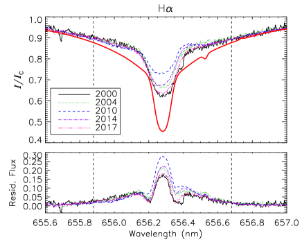
Figure 15: H$\alpha$ continuum-normalized flux (top), and residual flux (bottom) after subtraction of a photospheric model, at similar pulsation phases ($\phi\sim 0.75$) in successive epochs. The thick red line shows a model line profile disk-integrated with the appropriate pulsation velocity. Vertical dashed lines indicate the integration range for EW measurement.

Fig. 15 shows H$\alpha$ in 2000, 2004, 2010, 2014, and 2017, selected so as to share the same pulsation phase ($\phi=0.75\pm 0.03$). A synthetic line profile calculated using the physical parameters obtained in § 4 is overplotted as a thick line. Comparison of observed to synthetic line profiles demonstrates that emission is present at all epochs, although it is substantially weaker in the earlier CORALIE data. The agreement of H$\beta$ with the model is reasonable at all epochs, although there is also weak emission present in the line core (Fig. 4). Close analysis of the line core of H$\beta$ shows evidence of evolution, with the same trend as in H$\alpha$, although this evolution is of a much lower amplitude.

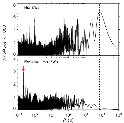
Figure 16: Periodogram for H$\alpha$ EWs (top), and after pre-whitening with the highest-amplitude period (bottom). The highest-amplitude period is indicated by the dashed line. The red arrow indicates the pulsation period determined from the RVs.

H$\alpha$ EWs were measured with an integration range of $\pm$0.4 nm of the rest wavelength in order to include only the region with emission (Fig. 15). The spectra were first shifted to a rest velocity of 0 km s^-1 by subtracting the RVs measured in § 3. The periodogram for these measurements is shown in the middle panel of Fig. 16. It shows a peak at 6700 d or 18 yr. The S/N of this peak is 29, indicating that it is statistically significant. This is consistent with the very long timescale of variation inferred from the ESPaDOnS $\langle B_{z}\rangle$ periodogram (Fig. 12), and with the minimum 7200 d period inferred from the positive and negative $\langle B_{z}\rangle$ extrema in the ESPaDOnS and MuSiCoS data.

The bottom panel of Fig. 13 shows the H$\alpha$ EWs as a function of time. Maximum emission and maximum $\langle B_{z}\rangle$ occur at approximately the same phase, as do the $\langle B_{z}\rangle$ minimum and the minimum emission strength. The variation in EW is seen more clearly in the annual mean EWs (open circles), which are tabulated in Table 2. The relative phasing of $\langle B_{z}\rangle$ and EW is consistent with a co-rotating magnetosphere, and supports the accuracy of the adopted period. Since $\langle B_{z}\rangle$ is both positive and negative, two local emission maxima are expected at the positive and negative extrema of the $\langle B_{z}\rangle$ curve, as at these rotational phases the magnetospheric plasma is seen closest to face on. The solid curve in the bottom panel of Fig. 13 shows a $2^{nd}$-order sinusoidal fit to the annual mean EWs, which indeed yields two local maxima, the strongest corresponding to $\langle B_{z}\rangle$$=$$\langle B_{z}\rangle$_max, and the second maximum predicted to occur at $\langle B_{z}\rangle$$=$$\langle B_{z}\rangle$_min. Note that, due to the incomplete phase coverage (less than half of a rotational cycle), in the event that the H$\alpha$ variation is indeed a double-wave a Lomb-Scargle periodogram should show maximum power at close to half of the rotational period. The periodogram peak at 18-yr would then indicate $P_{\rm rot}=36$ yr, consistent with the rotational period inferred from $\langle B_{z}\rangle$.

7.1.2 Short-term modulation

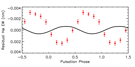
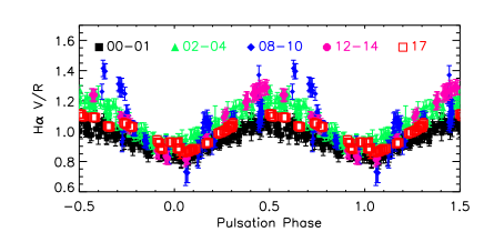
Figure 17: Top: residual H$\alpha$ EWs, after removal of the sinusoidal variation shown in the bottom panel of Fig. 13, phased with the pulsation period and binned with pulsation phase. The thick solid black line indicates the EW variation expected from a photospheric model calculated using the $\pm$300 K $T_{\rm eff}$ variation determined in § 4.5, normalized by subtracting the mean EW of the model. The amplitude of the residual EW variation is 3 times larger than predicted by the photospheric model, and is about 0.5 cycles out of phase. Bottom: H$\alpha$ V/R variation. Symbols and colors indicate the year of observation, the last two digits of which are given in the legend. The amplitude of the variation is much higher than predicted by the photospheric model, which is essentially flat on this scale and therefore is not shown. The amplitude furthermore changes between epochs, which is not expected for photospheric pulsations given the high stability of pulsation properties in other lines.

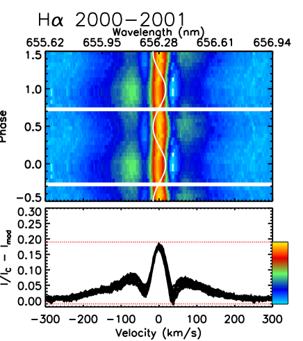
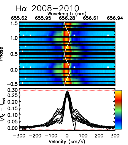
Figure 18: H$\alpha$ dynamic spectra in the epochs of minimum (2000-2001) and maximum (2008-2010) emission. The synthetic spectrum shown in Fig. 15 was used as a reference spectrum. Observed spectra were shifted to 0 km s^-1 by subtracting their RVs, and then co-added in 20 phase bins. The white curves indicate the RV curve due to pulsations. In all epochs, the emission profile has three components: a central peak near 0 km s^-1, which shifts slightly about line centre, but stays nearly constant in strength; a blue-shifted peak, which is at maximum strength at phase 0 and disappears by phase 0.5; and a red-shifted peak, which disappears at phase 0 and is at a maximum at phase 0.5. All three components increase in strength from 2000 to 2010. Note the greater amplitude of the variation in the secondary emission lobes in the 2008-2010 data.

As a first step to investigating whether H$\alpha$ is affected by pulsation, residual EWs were obtained by subtracting the least-squares 2^nd-order sinusoidal fit to the annual mean EWs. The bottom panel of Fig. 16 shows the period spectrum of the residual EWs. The strongest peak is at the stellar pulsation period, with a S/N of 12. After prewhitening the EWs with both the rotational and pulsational frequencies, the S/N of the highest peak in the periodogram is close to 4, suggesting that all significant variation is accounted for by these two frequencies.

While the semi-amplitude of the residual EW variation is similar to the median error bar, binning the residual EWs by pulsation phase does not change the semi-amplitude, but increases the significance of the variation to $\sim 8\sigma$ with respect to the mean error bar. The phase-binned residual EWs are shown phased with the pulsation period in the top panel of Fig. 17. There is a coherent variation of the phase-binned residual EWs with the pulsation period, with a semi-amplitude of approximately 0.003 nm.

One obvious candidate mechanism for producing this pulsational modulation is the change in the EW of the underlying photospheric profile due to the changing $T_{\rm eff}$, as explored in § 4.5. To investigate this hypothesis we calculated synthetic spectra via linear interpolation between the grid of tlusty BSTAR2006 models (Lanz & Hubeny, 2007). We used the physical parameters from § 4, including the $\pm$300 K $T_{\rm eff}$ variation found in § 4.5. Deformation of the line profile due to pulsation was accounted for using the RV curve from § 3, and modelling the (assumed radial) pulsations as described in § 4.1. Spectra were calculated at 20 pulsation phases, and the EW was measured at each phase using the same integration range as used for the observed data, and after moving the synthetic spectra to zero RV. The black line in the top panel of Fig. 17 shows the resulting variation, normalized by subtracting the mean EW across all models. The semi-amplitude of the EW variation expected due to changes in the photospheric profile due to pulsation is about 0.001 nm, much smaller than observed. Furthermore, it is out of phase with the observed variation by about 0.5 pulsation cycles. Note that the maximum and minimum EWs of the predicted variation correspond to the minimum and maximum of the $T_{\rm eff}$ variation (Fig. 7), as expected for H lines, which grow weaker with increasing $T_{\rm eff}$ in this $T_{\rm eff}$ range.

Radial pulsation introduces asymmetry into the line profile, which can be quantified by $V/R$, defined as the ratio of the EW in the blue half to the EW in the red half of the line. We measured $V/R$ from EWs calculated from $-$0.4 nm to line centre (defined at the laboratory rest wavelength shifted by the RV measured from metallic lines in § 3), and line centre to $+0.4$ nm. The bottom panel of Fig. 17 shows the $V/R$ variation. The semi-amplitude of the variation is about 0.25. This is much higher than the semi-amplitude of 0.0007 predicted by synthetic spectra calculated using a radially pulsating photospheric model; since this is essentially flat on the scale of Fig. 17, the photospheric variation is not shown. The low level of line asymmetry in the synthetic spectra is a consequence of the large Doppler broadening of the H$\alpha$ line, approximately 30 km s^-1 or about twice the semi-amplitude of the RV curve. For narrower lines, e.g. the C ii 656.3 nm line for which the Doppler velocity is similar to the RV semi-amplitude, the predicted and observed $V/R$ variations are in reasonable agreement.

The semi-amplitude of the H$\alpha$ $V/R$ variation increases steadily from 0.16 in 2000-2001, to 0.20 in 2002-2004, to 0.35 in 2008-2010, and then declines to 0.24 in 2012-2014 and 0.13 in 2017. This is the same pattern as the change in total emission strength, thus, the amplitude of the V/R variation correlates to the total emission strength and, therefore, to $\langle B_{z}\rangle$.

For a more detailed view of the pulsational modulation of H$\alpha$ we calculated dynamic spectra phased with the pulsation period. These are shown in Fig. 18, using the synthetic line profile from Fig. 15 as a reference spectrum. Individual line profiles were moved to 0 km s^-1 by subtracting their RVs, and then binned by pulsation phase using phase bins of 0.05 cycles. The two panels of Fig. 18 show dynamic spectra in the epochs of minimum emission (2000-2001) and maximum emission (2008-2010). The emission line morphology and pattern of variability is essentially identical in other epochs. In both cases, the emission peaks near the centre of the line. In the CORALIE data, the H$\alpha$ emission peak is $\sim$20% of the continuum. This rises to about 28% of the continuum in the ESPaDOnS data. The emission peak anticorrelates slightly with the RV, as shown by the overplotted white lines. The strong red and blue emission variability revealed by the $V/R$ variation in the bottom panel of Fig. 17 is due to secondary emission peaks which occur at phases 0.0 and 0.5, respectively blue- and red-shifted with respect to the line centre. As with the central emission peak, these are stronger in the ESPaDOnS data, reflecting the change in $V/R$ amplitude over time. Note that, in the data acquired at earlier epochs, these secondary emission bumps are apparently separated from the main emission peak, while in later epochs they are connected (although this depends on the choice of the reference spectrum).

Both the emission strength (as measured by the residual EWs after pre-whitening with the $2^{nd}$-order fit in Fig. 13) and the line asymmetry (as quantified by $V/R$) vary coherently with the pulsation phase. Synthetic photospheric spectra calculated using a radially pulsating model are unable to reproduce the residual EW variation, which is both 3$\times$ larger than predicted, and 0.5 cycles out of phase. The amplitude of the observed $V/R$ variation is about 300$\times$ larger than predicted by the model, which does not reproduce the prominent blue- and red-shifted secondary emission bumps. The amplitude of $V/R$ is furthermore variable with time, increasing and decreasing in strength in the same fashion as the total emission strength. As the star’s pulsation amplitude is extremely regular, a change in the amplitude of $V/R$ with epoch cannot be explained by photospheric pulsation. These discrepancies between model and observation suggest either that the origin of the pulsational modulation of H$\alpha$ is either not photospheric, or that it cannot be explained due to $T_{\rm eff}$ variation alone. Exotic processes, such as temperature inversions related to shockwaves produced by the star’s supersonic pulsations, may be one explanation. Alternatively, the origin of the pulsational modulation may reside within the magnetosphere.

7.2 UV emission lines

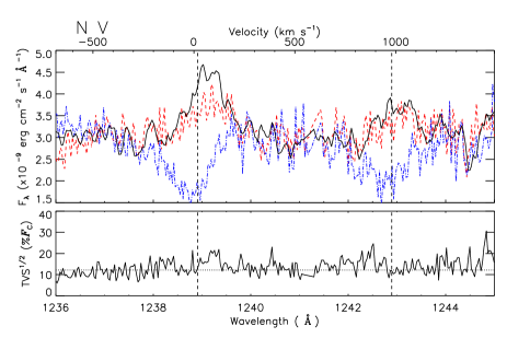
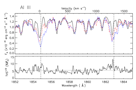
Figure 19: Comparison between the mean N v (top) and Al iii (bottom) emission lines of $\xi^{1}$ CMa (solid, black), and those of $\beta$ Cep at maximum emission (red, dashed) and maximum absorption (blue, dot-dashed). Vertical dashed lines indicate rest wavelengths. $\xi^{1}$ CMa’s emission lines are similar to those of $\beta$ Cep at maximum emission, albeit somewhat stronger. The lower panels show Temporal Variance Spectra (TVS, see text), calculated from all spectra, which characterize the variability of the spectra normalized to the continuum. The horizontal line indicates the continuum variation, in comparison to which there is no statistically significant variability inside the line profile.

Emission is present in four of the UV doublets often used to diagnose the wind properties of early-type stars: N v 1239, 1243 Å; Si iv 1394, 1403 Å; C iv 1548, 1551 Å; and Al iii 1854, 1863 Å. The emission profiles of these doublets are similar to those of the magnetic $\beta$ Cep pulsator $\beta$ Cep at maximum emission. Schnerr et al. (2008) performed this comparison for the C iv doublet. Fig. 19 compares the mean line profiles for $\xi^{1}$ CMa’s N v and Al iii lines to those of $\beta$ Cep, and demonstrates that these lines are also similar to those of $\beta$ Cep at maximum emission. Such emission is unique to magnetic stars, and as an indirect diagnostic of stellar magnetism has historically prompted the search for magnetic fields in such stars (e.g., Henrichs 1993; Henrichs et al. 2013; indeed, the detection of $\xi^{1}$ CMa’s UV emission motivated the collection of the MuSiCoS data).

The presence of emission in the N v line is particularly interesting. This line is not seen in normal early B-type stars (Walborn et al., 1995), nor is it present in most normal late O-type stars (e.g. Brandt et al. 1998). In their study of IUE data for 4 magnetic B-type stars, including $\beta$ Cep, Smith & Groote (2001) concluded that this doublet must be formed at $\sim$30 kK, somewhat higher than the photospheric $T_{\rm eff}$. The presence of N v lines in the UV spectra of relatively cool stars is thought to be a consequence of Auger ionization due to the presence of X-rays (Cassinelli & Olson, 1979). Since $\xi^{1}$ CMa has a strong magnetic field, it is expected to be overluminous in X-rays due to magnetically confined wind shocks, and is indeed observed to be overluminous in X-rays to the degree predicted by models (Oskinova et al., 2011; Nazé et al., 2014).

$\beta$ Cep’s wind lines show clear variability synchronized with its rotation period (Henrichs et al., 2013). In contrast, $\xi^{1}$ CMa’s wind lines show only a very low level of variability, more similar to that seen in a normal (magnetically unconfined) stellar wind (Schnerr et al., 2008). The bottom panels of Fig. 19 show Temporal Variance Spectra (TVS), which compare the variance within spectral lines to the variance in the continuum (Fullerton et al., 1996). To minimize variation due to pulsation, spectra were moved to 0 km s^-1 by subtracting the RV computed on the basis of the RV curve and ephemeris determined in Section 3. With the uncertainty in $P_{0}$ and in $\dot{P}$ (§ 3), the uncertainty in pulsation phase is about 0.028, corresponding to a maximum uncertainty in RV of 3 km s^-1, less than the $\sim$7.8 km s^-1 velocity pixel of the IUE data. RV correction reduces the TVS pseudocontinuum level by a factor of about 2 to 3.

Comparison of EW measurements of these lines to EWs of synthetic spectra, using the same radially pulsating model described above in § 7.1, yielded ambiguous results, due to the small number of high-dispersion IUE observations (13 spectra), and formal uncertainties similar to the maximum level of variability, $\sim$0.02 nm. This low level of variability is consistent with the weak variability of the residual H$\alpha$ EWs.

The lack of variability in $\xi^{1}$ CMa’s wind lines is consistent with a rotational pole aligned with the line of sight, an aligned dipole, a long rotation period, or some combination of these. The similarity to $\beta$ Cep’s emission lines at maximum emission suggests that the magnetic pole was close to being aligned with the line of sight when the UV data were acquired. The long-term modulations of both H$\alpha$ and $\langle B_{z}\rangle$ favour an oblique dipole with a long rotational period, in which case the UV data should have been acquired at a rotational phase corresponding to one of the extrema of the $\langle B_{z}\rangle$ curve. Phasing the UV data with the same 30 yr rotational period as in Fig. 13 yields a phase close to 1.0, i.e. they would indeed have been obtained close to magnetic maximum. Assuming that the data must have been acquired near an extremum of the $\langle B_{z}\rangle$ curve (i.e. at a phase close to 0.5 or 1.0) would require a period of 10, 15, 20, 30, or 60 years, of which only 30 and 60 years are not excluded by the magnetic data. This assumes that the UV data were, in fact, acquired close to an extremum. Given that the UV emission is only slightly stronger than that of $\beta$ Cep, which has a weaker magnetic field and no H$\alpha$ emission, it may be the case that the true maximum UV emission strength is significantly in excess of observations, in which case the UV data cannot be used to infer $P_{\rm rot}$.

8 Magnetic and magnetospheric parameters

In this section, the $\sim 30$ yr rotation period inferred from magnetic and spectroscopic data is used with the star’s physical parameters and $\langle B_{z}\rangle$ measurements to establish constaints on the properties of $\xi^{1}$ CMa’s surface magnetic field, circumstellar magnetosphere, and spindown timescales, using the self-consistent Monte Carlo method described by Shultz (2016). These results are summarized in Table 3.

Table 3: Magnetic, magnetospheric, and rotational properties. The final column gives the section in which the parameter is derived.

Parameter	Value	Ref.
$P_{\rm rot}$ (d)	$>$30 yr	6.1
$r$	-0.78$\pm$0.02	8.1
$\beta$ (∘)	83${}^{+5}_{-12}$	8.1
$\epsilon$	0.36$\pm$0.02	4.2
$B_{\rm d}$ (kG)	$>1.1$	8.1
$W$	$<7\times 10^{-5}$	8.2
$R_{\rm K}$ ($R_{*}$)	$>580$	8.2
$\log{\dot{M}}~{}(M_{\odot}~{}{\rm yr}^{-1})$	-8.0$\pm$0.1	8.2, Vink et al. (2001)
$v_{\infty}$ (km s-1)	2070$\pm$60	8.2, Vink et al. (2001)
$\eta_{*}$	$>340$	8.2
$R_{\rm A}$ ($R_{*}$)	$>4.6$	8.2
$\tau_{\rm J}$	4$\pm$1	8.3
$t_{\rm S,max}$	42$\pm$12	8.3

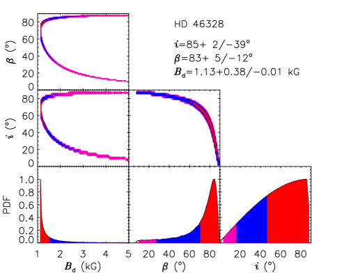
Figure 20: Oblique Rotator Model parameters determined via a Monte Carlo approach. Red, blue, and pink show the 1, 2, and 3$\sigma$ contours of the grid. The bottom panels show probability density functions (PDFs) for $B_{\rm d}$, $\beta$, and $i$, where $i$ was drawn from a random distribution over a solid angle of 4$\pi$.

The $\langle B_{z}\rangle$ variation of a rotating star with a dipolar magnetic field can be reproduced with a three-parameter model: the inclination angle $i$ between the rotational axis and the line of sight, the obliquity angle $\beta$ between the magnetic and rotational axes, and the polar strength of the magnetic dipole at the stellar surface $B_{\rm d}$. The two angular parameters are related via $\tan{\beta}=(1-r)/(1+r)\cot{i}$, where $r$ is the ratio defined by Preston (1967) as $r=(|B_{0}|-B_{1})/(|B_{0}|+B_{1})$, with $B_{0}$ and $B_{1}$ the mean and semi-amplitude of the sinusoidal fit to $\langle B_{z}\rangle$ when phased with $P_{\rm rot}$. We determined $r=-0.78\pm 0.02$ from the sinusoidal fit to the annual mean $\langle B_{z}\rangle$ measurements shown in the top panel of Fig. 13. In consequence these results rely on the 30-year period.

The degeneracy between $i$ and $\beta$ is usually broken by determining $i$ independently, e.g. from $v\sin i$, $P_{\rm rot}$, and $R_{*}$. Using this method Hubrig et al. (2011) found $i\sim 3^{\circ}$, however, this was based on their rotation period of 2.18 d, which was shown in § 6.2 to be incorrect. Indeed, the equatorial rotational velocity implied by a 30-year period, $v_{\rm eq}<0.04$ km s^-1, is much less than the upper limit on $v\sin i$ $<8$ km s^-1 found in § 4.1 (and indeed, much less than the 1.8 km s^-1 velocity resolution of ESPaDOnS data). Since $i$ cannot be constrained, we applied a probabilistic prior, requiring that $i$ be drawn from a random distribution over 4$\pi$ steradians such that $P(i)=1-\cos{i}$ (e.g., Landstreet & Mathys 2000). The corresponding probability density function (PDF) is shown in the bottom right panel of Fig. 20. The bottom middle panel shows the resulting PDF for $\beta$, which peaks at $83^{\circ}$. Despite the inverse relationship of $i$ and $\beta$ obtained for $r=-0.78$ (middle panel of Fig. 20), and the bias towards large $i$ in the prior, large $\beta$ are favoured overall. We note that we obtain a similar $\beta$ to that given by Hubrig et al. (2011), however this is simply a coincidence as their value was obtained with an incorrect rotation period and a very different value of the Preston $r$ parameter (0.56, as compared to -0.78).

For each ($i$, $\beta$) pair, $B_{\rm d}$ was determined using Eqn. 1 from Preston (1967). This also requires knowledge of the limb darkening coefficient $\epsilon$, which we obtained from the tables calculated by Díaz-Cordovés et al. (1995) as $\epsilon=0.36\pm 0.02$ (§4.1). The resulting PDF peaks sharply at the minimum value permitted by Preston’s equation, $B_{\rm d}=1.1$ kG. As demonstrated in the middle and upper left panels of Fig. 20, $B_{\rm d}<2$ kG over the range $20^{\circ}<i<85^{\circ}$, with a low-probability tail extending out to several kG for very large and very small $i$ and $\beta$. This is much lower than the value of $\sim$5.3 kG given by Hubrig et al. (2011), which arose from their very small $i$.

If instead the ESPaDOnS and MuSiCoS measurements define the extrema of $\langle B_{z}\rangle$, we obtain $r=-0.33\pm 0.02$. This does not affected $B_{\rm d}$, although a slightly smaller $\beta\sim 75^{\circ}$ is favoured.

Magnetic wind confinement is governed by the balance of kinetic energy density in the radiative wind to the magnetic energy density. This is expressed by the dimensionless wind magnetic confinement parameter $\eta_{*}$ (ud-Doula & Owocki, 2002). If $\eta_{*}>1$, the star possesses a magnetosphere.

Oskinova et al. (2011) analyzed IUE observations of $\xi^{1}$ CMa using the Potsdam Wolf-Rayet (PoWR) code in order to determine the wind parameters, obtaining $\log{(\dot{M}/M_{\odot}~{}{\rm yr^{-1}})}=-10$ and $v_{\infty}$$=700$ km s^-1. However, magnetic confinement reduces the net mass-loss rate and, more seriously, strongly affects line diagnostics due to the departure from spherical symmetry in the circumstellar environment. Indeed, Oskinova et al. were unable to achieve a simultaneous fit to the Si iv and C iv doublets. Comparison of magnetohydrodynamic (MHD) simulations and spherically symmetric models to the magnetospheric emission of Of?p stars has demonstrated that MHD simulations yield a superior fit, and require mass-loss rates comparable to those obtained from the Vink et al. (2001) recipe, whereas spherically symmetric models in general require much lower mass-loss rates to achieve a relatively poor match to the observations (Grunhut et al., 2012b; Marcolino et al., 2012, 2013). In addition to this, magnetic wind confinement is not expected to modify the surface mass flux, which is the relevant quantity in calculating the strength of magnetic confinement (ud-Doula & Owocki, 2002). Thus, $\eta_{*}$ should be determined using the wind parameters as they would be in the absence of a magnetic field, rather than those measured via spectral modelling (e.g., Petit et al. 2013). Using the mass-loss recipe of Vink et al. (2001) with $T_{\rm eff}$, $\log{L}$, and $M_{*}$ from Table 1, assuming the metallicity $Z/Z_{\odot}=1$, and determining the wind terminal velocity $v_{\infty}$$=2070\pm 60$ km s^-1 via scaling the star’s escape velocity by 2.6 as suggested by Vink et al., yields a mass-loss rate $\log{(\dot{M}/M_{\odot}~{}{\rm yr^{-1}})}=-8.0\pm 0.1$. From Eqn. 7 of ud-Doula & Owocki (2002), $\eta_{*}>340$, so the wind is magnetically confined.

The physical extent of the magnetosphere is given by the Alfvén radius $R_{\rm A}$, defined as the maximum extent of closed magnetic field lines in the circumstellar environment. $R_{\rm A}$ can be calculated heuristically from $\eta_{*}$ (Eqn. 7 in ud-Doula et al. 2008): we find $R_{\rm A}$ $>4.6~{}R_{*}$. Unless $i$ is particularly large or small, in which case $B_{\rm d}$ is significantly in excess of 2 kG, the magnetic and magnetospheric parameters will be close to the derived lower limits. $R_{\rm A}$ is almost certainly below 20 $R_{*}$.

$\xi^{1}$ CMa has the highest X-ray luminosity and the hardest X-ray spectrum of any of the magnetic $\beta$ Cep stars (Cassinelli et al., 1994; Oskinova et al., 2011). The X-ray luminosity, corrected for interstellar absorption corresponding to $E(B-V)=0.015$, is $2.4\times 10^{31}{\rm ergs^{-1}}$ (Nazé et al., 2014). Using 2D MHD simulations ud-Doula et al. (2014) calculated X-ray emission from magnetically confined wind shocks and developed an X-ray Analytic Dynamical Magnetosphere (XADM) scaling for $\log{L_{\rm X}}$ with $B_{\rm d}$, $R_{*}$, $\dot{M}$, and $v_{\infty}$. Comparison to available X-ray data for magnetic early-type stars has indicated that $\log{L_{\rm X}}$ predicted by XADM should be scaled by $\sim$5-20% to match the observed $\log{L_{\rm X}}$ (Nazé et al., 2014). This efficiency factor accounts for dynamical infall of the plasma. XADM successfully predicts the X-ray luminosity of magnetic, hot stars across 3 decades in $\log{L}$, 2 decades in $B_{\rm d}$, and 5 decades in $\log{L_{\rm X}}$ (Nazé et al., 2014), i.e. the range of the model’s successful application is much larger than the uncertainty introduced by the efficiency factor. Assuming an efficiency of 10%, $B_{\rm d}=1.1$ kG, and taking into account the uncertainties in the stellar parameters in Table 1, XADM predicts $\log{L_{\rm X}}$$=31.5\pm 0.1$, in excellent agreement with the observed X-ray luminosity $\log{L_{\rm X}}$$=31.47$. Adopting the higher value of $B_{\rm d}=5.3$ kG suggested by Hubrig et al. (2011) yields $\log{L_{\rm X}}$ $=31.7$, slightly higher than observed (although this can be reconciled by lowering the efficiency factor to 5%). If the lower $\dot{M}$ and $v_{\infty}$ determined by Oskinova et al. (2011) are used instead, XADM predicts $\log{L_{\rm X}}$ $=28.9$ with an efficiency factor of 100%, 2.6 dex lower than observed. Since the efficiency factor can only lower $\log{L_{\rm X}}$, it is impossible for the XADM model to match $\xi^{1}$ CMa’s observed X-ray luminosity with a mass-loss rate significantly lower than the Vink et al. (2001) prediction.

Petit et al. (2013) divided magnetic, massive stars into two classes, those with dynamical magnetospheres (DMs) only, and those also possessing centrifugal magnetospheres (CMs). CMs appear when $R_{\rm K}$ $<$ $R_{\rm A}$, where $R_{\rm K}$ is the Kepler radius, defined as the radius at which the centrifugal force due to corotation compensates for the gravitational force (Townsend & Owocki, 2005; ud-Doula et al., 2008). Solving for $R_{\rm K}$ using Eqn. 12 from Townsend & Owocki (2005) with $M_{*}$ from Table 1 and $P_{\rm rot}>30$ yr yields $R_{\rm K}$ $>580~{}R_{*}$. As $R_{\rm K}$ $\gg$ $R_{\rm A}$, the magnetosphere does not include a CM. The Kepler radius is related to the dimensionless rotation parameter $W\equiv v_{\rm eq}/v_{\rm orb}=R_{\rm K}^{-3/2}$, where $v_{\rm orb}$ is the velocity required to maintain a Keplerian orbit at the stellar surface (ud-Doula et al., 2008). Critical rotation corresponds to $W=1$, and no rotation to $W=0$. For $\xi^{1}$ CMa, $W<7\times 10^{-5}$.

Magnetic wind confinement leads to rapid spindown due to angular momentum loss via the extended moment arm of the magnetized wind (Weber & Davis, 1967; ud-Doula et al., 2009). The rotation period will decrease exponetially, with a characteristic angular momentum loss timescale $\tau_{\rm J}$ of (ud-Doula et al., 2009):

$$\tau_{\rm J}=\frac{3}{2}f\tau_{\rm M}\left(\frac{R_{*}}{R_{\rm A}}\right)^{2},$$ (2)

where $\tau_{\rm M}\equiv M_{*}/\dot{M}$ is the mass-loss timescale, and $f$ is the moment of inertia factor, which can be evaluated from the star’s radius of gyration $r_{\rm gyr}$ as $f=r_{\rm gyr}^{2}$. Consulting the internal structure models calculated by Claret (2004), $f\simeq 0.06$ for a star of $\xi^{1}$ CMa’s mass and age. Solving Eqn. 2 then yields $\tau_{\rm J}=4\pm 1$ Myr. The rotation parameter at a time $t$ after the birth of the star is

$$W(t)=W_{0}e^{-t/\tau_{\rm J}},$$ (3)

where $W_{0}$ is the initial rotation parameter. Assuming $W_{0}=1$ yields the maximum spindown age $t_{\rm S,max}=42\pm 12$ Myr (Petit et al., 2013). This is about 4 times longer than the age inferred from evolutionary tracks. Solving Eqn. 3 for $W_{0}$ yields $W_{0}<0.02$. Thus, either magnetic braking must have been much more rapid than predicted, or almost all of the star’s angular momentum loss must have occurred before it began its main sequence evolution, i.e. the star was already a slow rotator at the ZAMS.

Given the important role played by the mass-loss rate in determining $R_{\rm A}$ and $\tau_{\rm J}$, it is of interest to explore the sensitivity of these results to different mass-loss prescriptions. Muijres et al. (2012) found that they were unable to reproduce the observed mass-loss rates of stars with $\log{L}<5.2$, suggesting that $\dot{M}$ may be lower than predicted by the Vink et al. (2001) recipe. We first note that, since $\tau_{\rm J}$ increases with decreasing $\dot{M}$, a lower mass-loss rate cannot resolve the discrepancy between $t_{\rm S,max}$ and the age inferred from the HRD. Second, we note that satisfying the condition for a CM ($R_{\rm A}$$>$$R_{\rm K}$) requires $\log{(\dot{M}/M_{\odot}~{}{\rm yr^{-1}})}\leq-16.5$. If the lower $\dot{M}$ and $v_{\infty}$ found by Oskinova et al. (2011) are used to calculate the magnetospheric and spindown parameters, none of the above conclusions are fundamentally changed ($R_{\rm A}$ $\sim 14~{}R_{*}\ll R_{\rm K}$ , and $t_{\rm S,max}=250^{+80}_{-100}$ Myr). Lucy (2010) computed mass-loss rates for late O-type stars in the weak-wind domain using the theory of reversing layers (Lucy, 2007), and for a star with $\xi^{1}$ CMa’s $T_{\rm eff}$ and $\log{g}$ predict $\log{(\dot{M}/M_{\odot}~{}{\rm yr^{-1}})}\sim-8.8$. Krtička (2014) provided an alternate calculation for $\dot{M}$, intended specifically for B-type stars, and for $\xi^{1}$ CMa predicted $\log{(\dot{M}/M_{\odot}~{}{\rm yr^{-1}})}=-8.9$ (see Table 5 in Krtička 2014), similar to the Lucy (2010) prediction. Thus, while there are systematic differences between theoretical mass-loss rates, these are much smaller than would be required to change the basic conclusions that the star lacks a CM and has a spindown age much less than its evolutionary age.

9 Discussion

9.1 Impact of pulsation on the magnetometry

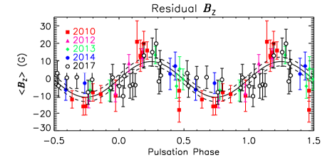
Figure 21: Residual ESPaDOnS $\langle B_{z}\rangle$ measurements, after subtraction of the mean $\langle B_{z}\rangle$ at each epoch, phased with the pulsation period. The legend indicates the year in which each dataset was acquired. Only epochs with at least 4 observations are shown.

Figure 22: Stokes $I$ (left), null $N$ (middle), and Stokes $V$ (right) LSD profiles. Observed profiles are shown by black circles, synthetic profiles by red lines.

While $\langle B_{z}\rangle$ exhibits a clear long-term modulation, it also shows evidence for short-term variability. In particular in 2010 (HJD$\sim$2455200), the most densely time-sampled epoch, there is substantial apparent scatter in the measurements: the mean error bar is 5 G, but the standard deviation of $\langle B_{z}\rangle$ in this epoch is 15 G.

We calculated residual $\langle B_{z}\rangle$ measurements by subtracting the mean $\langle B_{z}\rangle$ at each annual epoch in order to remove the long-term trend. These are shown phased with the pulsation period in Fig. 21. The reduced $\chi^{2}$ of a least-squares sinusoidal fit to all residual $\langle B_{z}\rangle$ measurements is 1.2, as compared to 2.8 for the null hypothesis of no variation. In 2010 there is an apparently coherent variation with a semi-amplitude of 16$\pm$2 G, consistent with the standard deviation in $\langle B_{z}\rangle$ of 15 G, and 3 times larger than the median error bar of 5 G. The reduced $\chi^{2}$ of the least-squares sinusoidal fit to the 2010 residual $\langle B_{z}\rangle$ measurements is 0.9, as compared to 6.1 for the null hypothesis. In 2017, the epoch with the largest number of observations and the most systematic sampling of the phase curve, the same fit yields a semi-amplitude of 7$\pm$2 G, which is identical to both the standard deviation of, and the median uncertainty in, $\langle B_{z}\rangle$ during this epoch. The reduced $\chi^{2}$ of a sinusoidal fit and the null hypothesis to the 2017 data is close to 1 in both cases, indicating that in 2017 there is no evidence for a coherent variation with pulsation phase. In 2013, the only other epoch with sufficient observations to constrain a sinusoidal fit, the semi-amplitude is 10$\pm$5 G, the reduced $\chi^{2}$ of the fit is 1.3, and the reduced $\chi^{2}$ of the null hypothesis is 2.3, i.e. 2013 yields results intermediate between 2010 and 2017. This suggests that the observed variation of $\langle B_{z}\rangle$ may be explained as the superposition of a short-term variation with the stellar pulsation period on top of the long-term variation due to rotation, with the short-term variation declining in amplitude with $\langle B_{z}\rangle$.

We next turn our attention to the LSD profiles. It is clear from the numerous ‘definite’ detections in LSD $N$ profiles that pulsation has affected our data to some degree. Signatures in $N$ profiles are sometimes seen in stars in which the stellar lines vary during acquisition of the polarized sub-exposures used to construct the final Stokes $V$ spectrum. Following the analysis performed by Neiner et al. (2012), we modelled the $N$ profiles by creating disk-integrated Stokes $I$ and $V$ profiles at the radial velocities corresponding to the pulsation phases of each sub-exposure, and then combining the individual model profiles in such a way as to simulate the double-ratio method’s combination of $I\pm V$ beams to yield Stokes $I$, Stokes $V$, and $N$ (Donati et al., 1997). Each model profile was created with $v\sin i$$~{}=0$ km s^-1, a macroturbulent velocity of 8 km s^-1, the measured RVs, a projection factor of 1.45, and a constant dipolar magnetic field with $i=\beta=90^{\circ}$ and $B_{\rm d}$$=1.1$ kG, with the positive magnetic pole at the centre of the stellar disk. The model profiles were normalized to the observed Stokes $I$ EW.

Illustrative results are shown for Stokes $I$, $N$, and Stokes $V$ in Fig. 22. The model reproduces the variation in $N$ reasonably well. We conclude from this that the $N$ profile signatures are principally a consequence of line profile variability between sub-exposures.

There is no change in $\langle B_{z}\rangle$ measured from model LSD profiles created with or without introducing RV shifts between sub-exposures. Furthermore, $\langle N_{z}\rangle$ remains null, as expected. This result is in agreement with the observational results of Neiner et al. (2012), who found that while shifting sub-exposures by their pulsation velocities greatly reduced the $N$ profile signatures, $\langle B_{z}\rangle$ remained unchanged within error bars.

If the modulation of $\langle B_{z}\rangle$ with pulsation phase is not a consequence of an instrumental effect, it might be due to a real change in the intrinsic surface magnetic field strength of the star. An obvious mechanism that might produce such an effect is conservation of magnetic flux throughout radial pulsation cycles. Magnetic flux is conserved as $1/R_{*}^{2}$, and the semi-amplitude of the change in stellar radius is $\Delta r/R_{*}\sim 1-1.5\%$, thus $\langle B_{z}\rangle$ could vary by about $\pm$2–3% or $\pm 7-10$ G at $\langle B_{z}\rangle$${}_{\rm max}=328$ G, which is close to the observed semi-amplitude in 2010 of 16$\pm$2 G. In this scenario, maximum $\langle B_{z}\rangle$ should occur at phase 0.25, when the star is at its most contracted, and minimum $\langle B_{z}\rangle$ at phase 0.75, when the star is at its most extended; this is indeed what is observed. Thus, a modulation of $\langle B_{z}\rangle$ arising due to an actual change in the surface magnetic field strength with the pulsation period is consistent with both the magnitude and the phasing of the observed effect. The apparent proportionality of the semi-amplitude of the pulsational modulation of $\langle B_{z}\rangle$ to the magnitude of $\langle B_{z}\rangle$ is also consistent with this hypothesis, as a change in $\langle B_{z}\rangle$ due to a change in $B_{\rm d}$ should be largest when there is the least amount of magnetic flux cancellation across the stellar disk (i.e. at magnetic maximum).

While our model does not predict a change in $\langle B_{z}\rangle$ due to RV shifts between subexposures, we cannot entirely rule out the possibility that the modulation shown in Fig. 21 is due to line profile variability. Whatever its origin, the influence of pulsation on $\langle B_{z}\rangle$ is much smaller than the long-term modulation of $\langle B_{z}\rangle$, thus the fundamental conclusion that $P_{\rm rot}>30$ yr should not be affected by pulsation.

9.2 Does extremely slow rotation in an evolved magnetic B-type star make sense?

Due to magnetic braking evolved magnetic hot stars are expected to rotate more slowly than either similar, younger magnetic stars or non-magnetic stars of comparable age and mass. However, as was shown in § 8, the spindown age inferred for $\xi^{1}$ CMa is difficult to reconcile with the age inferred from its position on the HRD. The Ekström et al. (2012) evolutionary models imply an age of 11$\pm$0.7 Myr, while its spindown timescale is $\tau_{\rm J}=4\pm 1$ Myr. Thus, at most two or three e-foldings of the initial rotational period can have occurred since the ZAMS. Assuming initially critical rotation, $\xi^{1}$ CMa should now have a rotational period of about 6 d; conversely, calculating from its actual rotation period, its initial rotation fraction $W_{0}$ must have already been very close to 0, implying a rotational period on the ZAMS already on the order of years.

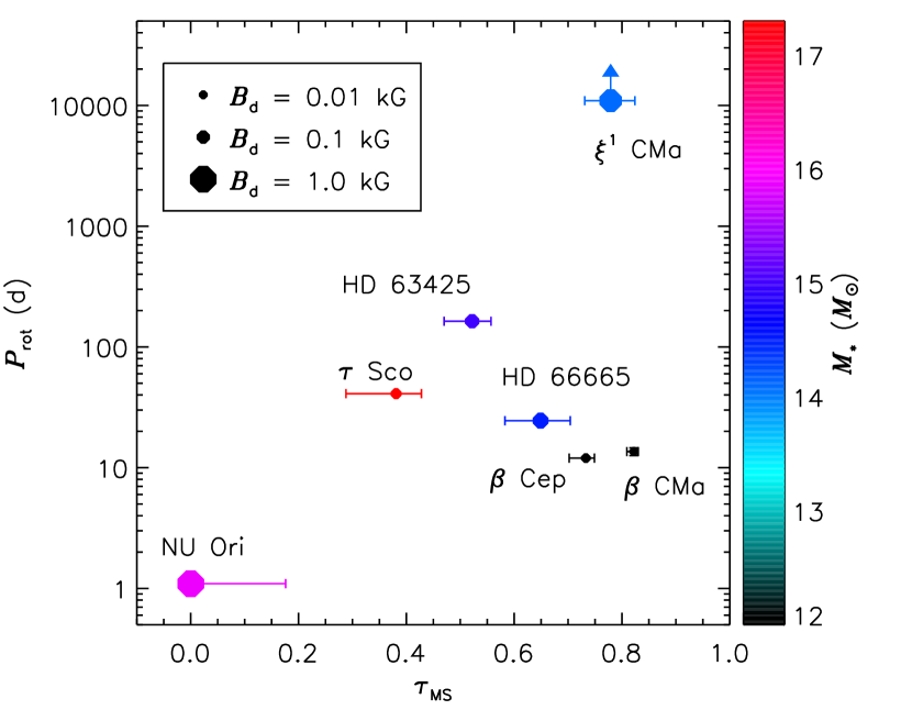
Figure 23: $P_{\rm rot}$ as a function of fractional main sequence age $\tau_{\rm MS}$ for magnetic early B-type stars with masses similar to $\xi^{1}$ CMa, with colour corresponding to stellar mass and symbol size to $B_{\rm d}$. Uncertainties in $P_{\rm rot}$ are negligible on the scale of the diagram.

Petit et al. (2013) calculated spindown ages for all stars in Fig. 8 except $\beta$ CMa and $\epsilon$ CMa, finding $40<t_{\rm S,max}<130$ Myr for these stars, i.e. their maximum spindown ages are 4 to 10 times greater than their main-sequence ages, which for stars in this mass range are typically 8 to 15 Myr. We note that the rotational periods of $\tau$ Sco and $\beta$ Cep are both known to high precision (Donati et al., 2006; Henrichs et al., 2013). For $\tau$ Sco, $t_{\rm S,max}=126^{+16}_{-32}$ Myr, while its position on the HRD indicates $t=3.3^{+0.5}_{-1.1}$ Myr, a discrepancy of 1.6 dex; similarly for $\beta$ Cep, $t_{\rm S,max}=204^{+9}_{-19}$ Myr, differing by 1.2 dex with its age of $t=13.2^{+0.4}_{-0.7}$ Myr (Shultz, 2016).

These discrepancies between the stellar age and the maximum spindown age cannot be reconciled by utilizing a different set of evolutionary models: while the absolute ages inferred from different prescriptions vary depending on assumptions about rotation, mixing, or mass-loss, these uncertainties in the models are typically on the order of 1 to 2 Myr for a 15 $M_{\odot}$ star, much less than the $\sim$1 dex difference between gyrochronological and evolutionary ages. It should be noted that the Ekström et al. (2012) models do not include magnetic fields. Fully self-consistent evolutionary models of magnetic stars are not yet available; however, it seems unlikely that such models will resolve the discrepancy via modification of the age inferred from a star’s position on the HRD.

Fossati et al. (2016) also found that spindown timescales are typically much longer than stellar ages for magnetic, massive stars, which they interpreted as evidence for rapid magnetic flux decay. At first order, the surface magnetic field should weaken as $1/R_{*}^{2}$ due to conservation of fossil magnetic flux. As an evolved star, $\xi^{1}$ CMa’s radius has increased by a factor of 1.8$\pm$0.1 since the ZAMS, thus its minimum surface magnetic field strength on the ZAMS should have been $B_{\rm d,ZAMS}>3.2$ kG. Recalculating $\tau_{\rm J}$ on the ZAMS using Vink mass-loss rates suggests that $\tau_{\rm J}$ should not have been very different from its present value, as the lower mass-loss rate on the ZAMS compensates for the stronger magnetic field and greater Alfvén radius. Thus, magnetic flux conservation alone cannot account for $\xi^{1}$ CMa’s slow rotation, and some other mechanism or combination of mechanisms – magnetic flux decay, rapid angular momentum loss on the PMS, or modification of the internal structure of the star due to the magnetic field – is necessary. While it is of course possible that the theoretical mass-loss rates are simply incorrect, resolving the discrepancy by changing $\dot{M}$ alone would require an increase of $\sim$1 dex, well outside the range of uncertainty of current models which typically differ a factor of 2 to 3, and are in addition usually lower than the Vink et al. (2001) mass-loss rates (e.g., Sundqvist et al. 2014; Keszthelyi et al. 2017).

The irreconcilability of gyrochronological and evolutionary timescales amongst magnetic early B-type stars is worthy of future investigation. Here, it is pointed out primarily to emphasize that the difficulty in explaining $\xi^{1}$ CMa’s extremely slow rotation should not count as an argument against a long rotational period, as this problem is shared by all similar stars.

Fig. 23 shows $P_{\rm rot}$ as a function of fractional main sequence age $\tau_{\rm MS}$ for those stars from Fig. 8 for which both $P_{\rm rot}$ and $B_{\rm d}$ are known. The majority of the dipolar field strengths and rotational periods were obtained from the catalogue published by Petit et al. (2013), and references therein. $\beta$ CMa’s magnetic, rotational, and stellar properties were obtained from Fossati et al. (2015a). The rotational periods of NU Ori and HD 63425 were determined using ESPaDOnS data (Shultz, 2016). Masses and fractional main sequence ages were determined via linear interpolation between the Ekström et al. (2012) evolutionary models on the basis of the stars’ positions on Fig. 8. For HD 63425 and HD 66665, we used the $T_{\rm eff}$-$\log{g}$ diagram to infer stellar parameters, as the uncertainties in $\log{L}$ are very large for these stars.

In addition to having by far the longest rotational period of any magnetic B-type star, $\xi^{1}$ CMa has a stronger magnetic field than any star in Fig. 23 but NU Ori. It is also amongst the most evolved stars in the sample: the only stars of a comparable fractional age are $\beta$ Cep and $\beta$ CMa, both of which are less massive ($\sim$12 $M_{\odot}$), and have much weaker magnetic fields ($\sim$0.1 kG). Since mass-loss rates increase with $M_{*}$, more massive stars should spin down more rapidly than less massive stars. With the exception of NU Ori, stars more massive than $\xi^{1}$ CMa all have rotational periods of 10-100 d, although they are less evolved. NU Ori, which has a stronger magnetic field, a much shorter rotational period, and a slightly higher stellar mass than $\xi^{1}$ CMa, is also the youngest star on the diagram, likely accounting for its rapid rotation. This comparison shows that, viewed in the context of stars with similar magnetic and stellar parameters, $\xi^{1}$ CMa’s very slow rotation is not anomalous given its age.

9.3 A B-type star with an optically detectable dynamical magnetosphere?

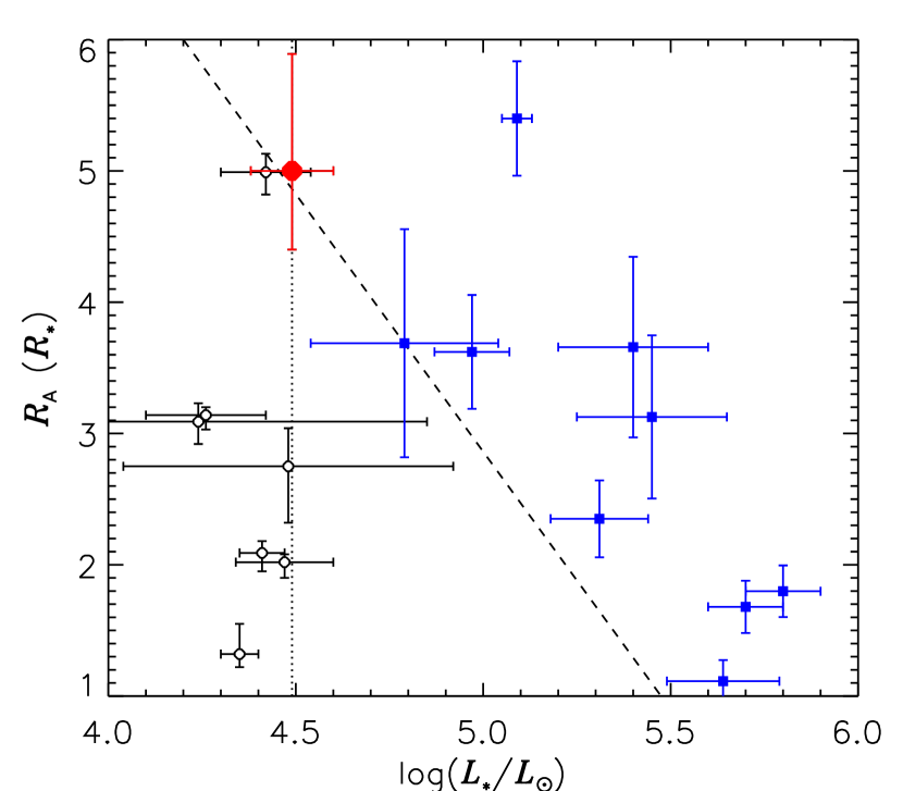
Figure 24: $R_{\rm A}$ as a function of $\log{L}$ for magnetic early B-type stars (open black circles) and the magnetic O-type stars (solid blue squares). $\xi^{1}$ CMa is shown as a large, filled red circle. With the exception of $\xi^{1}$ CMa, only the O-type stars display emission in H$\alpha$. The ad-hoc dashed line suggests a possible relationship between the onset of emission in DMs, and $R_{\rm A}$ and $\log{L}$.

In DMs, plasma deposited in the magnetosphere by the stellar wind falls back due to gravity, while in CMs centrifugal support due to the magnetically enforced corotation of the plasma with the star prevents infall above $R_{\rm K}$. Petit et al. (2013) noted that stars without CMs only display emission if their mass-loss rates are high enough to replenish the magnetosphere on dynamical timescales, thus enabling the circumstellar environment to remain optically thick despite continuous depletion as material returns to the photosphere. As a consequence, the only stars with optical emission lines originating in their DMs are the magnetic O-type stars, whereas the only magnetic B-type stars listed by Petit et al. as hosting H$\alpha$ emission possess CMs. While they were aware of $\xi^{1}$ CMa’s H$\alpha$ emission, Petit et al. assumed the 4.26 d rotation period found by Fourtune-Ravard et al. (2011), and thus that the emission originated in the star’s CM. However, as $R_{\rm K}$ $\gg$ $R_{\rm A}$, $\xi^{1}$ CMa does not have a CM.

The H$\alpha$ emission profile shown in Fig. 18 is furthermore entirely distinct from the double-horned profile characteristic of a CM, which generally produces two emission peaks located at approximately $\pm$$R_{\rm K}$ (e.g. Leone et al. 2010; Oksala et al. 2012; Grunhut et al. 2012a; Rivinius et al. 2013). The strong central peak is much more similar to the typical profile of a magnetic O-type star with a DM (e.g. Sundqvist et al. 2012; ud-Doula et al. 2013; Wade et al. 2015), although the emission peaks of such stars tend to be slightly red-shifted, whereas $\xi^{1}$ CMa’s is closer to line centre. $\xi^{1}$ CMa’s ultraviolet emission line morphology is also consistent with an origin in a DM, at least insofar as it is very similar to the emission lines of $\beta$ Cep, which does not have a CM.

This leads to the question of how a B-type star can have an optically detectable DM. The quantity of plasma in a DM is a function of two parameters: the size of the magnetosphere, and the mass-loss rate which feeds it. As is clear from Fig. 8, $\xi^{1}$ CMa is one of the most luminous magnetic B-type stars known: while $\tau$ Sco and NU Ori have similar $\log{L}$, no stars are known to have a higher luminosity. In Fig. 24 $R_{\rm A}$ is plotted as a function of $\log{L}$ for the stars in Fig. 8. Not only does $\xi^{1}$ CMa have a higher luminosity than most of the B-type stars, it also has one of the largest Alfvén radii.

Also plotted on Fig. 24 are the magnetic O-type stars from the Petit et al. (2013) catalogue. All of these stars have emission, despite the very small $R_{\rm A}$ of the stars with higher luminosities. The dashed diagonal line indicates a possible division between stars with and without emission line DMs. Under the assumption that a star with a smaller $R_{\rm A}$ requires a higher mass-loss rate in order to show emission, stars above the line should show emission, while those below should not. Alternatively, the presence or absence of emission could be related purely to the mass-loss rate, as indicated by the vertical dotted line: in this case, stars with $\log{L/L_{\odot}}\gtrsim 4.5$ should show emission. $\xi^{1}$ CMa’s position in either case is consistent with the presence of H$\alpha$ emission. The presence or absence of magnetospheric emission in magnetic OB stars with $4.5\leq\log{L/L_{\odot}}\leq 5.0$, but $R_{\rm A}$ $\geq 3~{}R_{*}$, would help to distinguish between these scenarios.

Only one other magnetic B-type star, NU Ori, is in the same part of the diagram as $\xi^{1}$ CMa. As noted above, NU Ori is a rapid rotator, and possesses a CM. This star shows neither H$\alpha$ nor UV emission (Petit et al., 2013). The absence of emission, given its high luminosity and comparable magnetic confinement strength to $\xi^{1}$ CMa, is a distinct puzzle deserving of future investigation.

9.4 A pulsating magnetosphere?

Due to the limited number and quality of IUE observations, the evidence for pulsational modulation of UV resonance doublets is inconclusive. Evidence for pulsational modulation of the star’s H$\alpha$ emission is much stronger. The residual H$\alpha$ EWs, after subtraction of a sinusoidal fit to the annual mean EWs phased with the presumed rotation period, yield a clear peak in the periodogram at the pulsation period. When phased with the pulsation period, the amplitude of the residual EW variation is 3 times higher than the amplitude expected from a photospheric modulation of the absorption line’s EW, and is furthermore 0.5 pulsation cycles out of phase with the predicted photospheric variation. Finally, H$\alpha$ shows a much stronger V/R variation than is predicted by the photospheric model.

Stochastic changes in the EW of the H$\alpha$ line have been observed for some magnetic O-type stars with dynamical magnetospheres, e.g. the well-studied object $\theta^{1}$ Ori C (Stahl et al., 2008). 3D MHD simulations are able to reproduce this short-term variability as a consequence of turbulent plasma infall (ud-Doula et al., 2013). As $\dot{M}$ is constant for such stars, their short-term variability is wholly a consequence of the complex behaviour of MHD plasmas. Since $\xi^{1}$ CMa’s mass-loss rate should change with the pulsation phase, it is conceivable that this could force a periodicity in the outflow and infall of the magnetically confined plasma. The observation of prominent blue- and red-shifted secondary peaks in the H$\alpha$ emission structure occuring at distinct pulsation phases, together with the stronger modulation in H$\alpha$ $V/R$ as compared to residual H$\alpha$ EWs, further suggests that, throughout the course of a pulsation cycle, there are larger local changes in the distribution of plasma within the magnetosphere, as compared to the total mass of magnetically confined plasma.

The majority of the H$\alpha$ emission is expected to be produced in the innermost regions (ud-Doula et al., 2013). The wind flow timescale, calculated using a standard $\beta=1$ velocity law, ranges from $\sim$0.13 d at a distance of 2 $R_{*}$, to $\sim$0.19 d at the minimum Alfvén radius of 4.6 $R_{*}$. The free-fall timescale is somewhat longer, ranging from 0.2 to 1.2 d over this same distance. These timescales are similar to the pulsation period, suggesting that periodic density waves arising due to the varying mass-loss rate might lead to a periodicity in the plasma infall. The strongest blue-shifted secondary emission peak occurs at about phase 1.0, and the strongest secondary red-shifted emission peak at phase 0.5. If the blue- and red-shifted emission peaks are respectively consequences of outflowing and infalling plasma, and assuming the majority of the emission is formed relatively close to the star, a lag of approximately 0.7 cycles between the peak mass-loss rate (at phase 0.3) and the strongest blue-shifted emission (at phase 1.0) would make sense.

While no other magnetic, massive star’s H$\alpha$ emission has ever been found to be modulated by pulsation as well as rotation, Oskinova et al. (2014) reported that $\xi^{1}$ CMa’s X-ray light curve exhibits a coherent variation with the pulsation period, with both hard and soft X-ray emission peaking $\sim$0.1 cycles after the maximum of the visible light curve.

Since $\xi^{1}$ CMa is a pulsating star, $\dot{M}$ is not constant. The changes in $T_{\rm eff}$ and $\log{L_{*}}$ should lead to a variation in $\dot{M}$ with a semi-amplitude of 0.05 dex. Changes in $v_{\infty}$ should be negligible. Calculation of $\eta_{*}$ and $R_{\rm A}$ as a function of pulsation phase suggests the overall changes in these parameters to be small ($\sim$20% in $\eta_{*}$ and 4% in $R_{\rm A}$). Similar X-ray pulsations have also been reported for the $\beta$ Cep star $\beta$ Cru (Cohen et al., 2008). As $\beta$ Cru does not have a detected magnetic field (J. Grunhut, priv. comm.), this argues against a purely magnetic explanation for the X-ray variability.

Oskinova et al. (2014) considered a variation in $\dot{M}$ as a possible mechanism behind the star’s X-ray pulsations, and rejected it based upon the absence of X-ray pulsations in other $\beta$ Cep stars, either magnetic or not. However, they did not consider their results in the context of the XADM model. The XADM model predicts a modulation in $\log{L_{\rm X}}$ of approximately $\pm 10$% to arise from a variation in $\dot{M}$ of $\pm$0.05 dex, with the maximum and minimum of the predicted X-ray light curve corresponding to the maximum and minimum of the visible light curve. This is the same amplitude as that reported by Oskinova et al. (2014).

As a sanity check, we performed similar calculations for $\beta$ Cep and $\beta$ Cen, the only other magnetic $\beta$ Cep stars with X-ray light curves. $\beta$ Cep is slightly cooler ($T_{\rm eff}$$\sim$26 kK), less strongly magnetized ($B_{\rm d}\sim 260$ G; Henrichs et al. 2013), and has somewhat lower amplitude pulsations leading to a smaller change in luminosity ($\pm$0.015 mag and $\pm$0.006 dex, respectively, as evaluated by phasing the star’s Hipparcos observations with its primary pulsation period of 0.19 d; Shibahashi & Aerts 2000) and, hence, a smaller change in the mass-loss rate ($\pm$0.03 dex). The XADM model predicts that $\beta$ Cep should have X-ray pulsations with a semi-amplitude of $\leq 6$%, close to the upper limit determined by Favata et al. (2009). For $\beta$ Cen, it is not clear which of the many pulsation frequencies identified by Pigulski et al. (2016) belongs to the magnetic secondary. However, even the highest amplitude frequency ($\pm$0.0015 mag) leads to a luminosity modulation of just 0.006 dex, hence a change in $\dot{M}$ of less than $\pm$0.01 dex, and, with $B_{\rm d}=200$ G (Shultz, 2016), a variation in the X-ray luminosity of $<3$%, below the upper limit established by Raassen et al. (2005).

It is probably not the case that simple calculation of global parameters at each pulsation phase provides an accurate picture. Strong local density variations due to the changing $\dot{M}$ may lead to correspondingly strong local changes in the magnetic confinement strength. Magnetohydynamic simulations will be necessary to properly explore the impact of stellar pulsation on magnetospheric dynamics.

10 Conclusions and Future Work

The principal result of this paper is that both magnetic and spectroscopic data indicate that the rotation period of $\xi^{1}$ CMa is very long, on the order of decades. Rotational periods on the order of days, as previously suggested in the literature, are conclusively ruled out by the ESPaDOnS $\langle B_{z}\rangle$ measurements alone, which require a period of at least 5100 d. Inclusion of the MuSiCoS results requires that $P_{\rm rot}$ be about 30 years, a conclusion supported by the modulation of the H$\alpha$ emission strength seen in the CORALIE and ESPaDOnS datasets. A period of approximately 30 years is consistent with the timing of the star’s strong UV emission, which should correspond to an extremum of the $\langle B_{z}\rangle$ curve. Given that phase coverage of the rotational cycle is incomplete to an unknown degree, the constraints that can be placed upon the geometry and strength of the magnetic field are necessarily somewhat loose. Further spectropolarimetric observation over decades is essential to characterization of the magnetic field. If the 30-year period is correct, magnetic crossover ($\langle B_{z}\rangle$$=0$) will occur in 2018, and magnetic minimum in 2025.

We have conducted the first detailed examination of the star’s weak H$\alpha$ emission, which we detect in all available spectroscopic data. There is no evidence in the interferometric data of a binary companion, and combined constraints from interferometry and RV residuals rule out a binary companion of sufficient luminosity to host the weak emission. Furthermore, there is no indication of a Keplerian disk in the high-resolution AMBER spectro-interferometry. Thus, the interferometric data does not support the hypothesis that the emission originates in the Keplerian disk of a classical Be companion star, indicating that this emission is produced in $\xi^{1}$ CMa’s circumstellar environment. This makes $\xi^{1}$ CMa the first magnetic $\beta$ Cep star with a magnetosphere detectable in visible light. Given that its extremely slow rotation implies a dynamical rather than a centrifugal magnetosphere, $\xi^{1}$ CMa is also the coolest star with a dynamical magnetosphere detectable in H$\alpha$.

Finally, in addition to the already reported modulation of X-ray flux with the pulsation period, the H$\alpha$ emission also appears to correlate with the pulsations in a fashion that seems likely to be intrinsic to the circumstellar plasma. The best evidence for this is in the strong H$\alpha$ $V/R$ variations, which are much greater than expected from a radially pulsating photospheric model. The total H$\alpha$ EW in any given epoch also varies in antiphase with the expected EW variation due to photospheric $T_{\rm eff}$ variation, and furthermore has a larger amplitude than predicted by a photospheric model. However, the EW is only weakly variable compared to $V/R$, suggesting that the distribution of plasma within the magnetosphere, rather than the total quantity of magnetically confined material, is the primary origin of the variability. Given the complex velocity fields within dynamical magnetospheres, magnetohydrodynamic (MHD) simulations will be necessary to understand the interplay between pulsation, mass-loss, and magnetic confinement. As the magnetic wind confinement parameter $\eta_{*}$ is on the order of 10², modeling $\xi^{1}$ CMa’s magnetosphere should be within the capabilities of the current generation of 2D MHD codes.

We also find a weak modulation of $\langle B_{z}\rangle$ with the pulsation period. Further modeling is needed to understand the origin of this phenomenon. Signatures in the diagnostic null profile are accurately reproduced as a consequence of RV variations between subexposures, however, this model does not predict any modulation of $\langle B_{z}\rangle$. Polarized radiative transfer in a moving atmosphere will be essential to answering the question of whether these modulations are an artefact of the measurement methodology, or intrinsic to the stellar magnetic field.

Acknowledgements The authors acknowledge the assistance of Conny Aerts, who provided the CORALIE dataset. This work has made use of the VALD database, operated at Uppsala University, the Institute of Astronomy RAS in Moscow, and the University of Vienna. MS acknowledges the financial support provided by the European Southern Observatory studentship program in Santiago, Chile. MS and GAW acknowledge support from the Natural Science and Engineering Research Council of Canada (NSERC). CN and the MiMeS collaboration acknowledge financial support from the Programme National de Physique Stellaire (PNPS) of INSU/CNRS. We acknowledge the Canadian Astronomy Data Centre (CADC). The IUE data presented in this paper were obtained from the Multimission Archive at the Space Telescope Science Institute (MAST). STScI is operated by the Association of Universities for Research in Astronomy, Inc., under NASA contract NAS5-26555. Support for MAST for non-HST data is provided by the NASA Office of Space Science via grant NAG5-7584 and by other grants and contracts. This project used the facilities of SIMBAD and Hipparcos. This research has made use of the Jean-Marie Mariotti litpro service co-developed by CRAL, IPAG, and LAGRANGE.

Appendix A Reliability of MuSiCoS data

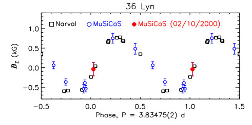
Figure 25: $\langle B_{z}\rangle$ measurements of 36 Lyn obtained with Narval and MuSiCoS, phased with the ephemeris determined from the MuSiCoS data by Wade et al. (2006). The MuSiCoS measurement obtained during the same observing run as the $\xi^{1}$ CMa observations is indicated by the filled red circle.

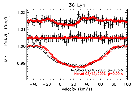
Figure 26: Comparison between the MuSiCoS LSD profile of the magnetic Bp star 36 Lyn obtained during the same observing run as the $\xi^{1}$ CMa data, and a Narval LSD profile of 36 Lyn at a similar rotational phase.

Fossati et al. (2015b) objected to a long rotation period, first suggested by Shultz et al. (2015), on the grounds that the period is largely constrained by the MuSiCoS measurements, and further suggesting that as these data were collected at high airmass the measurements were unreliable. As we have shown, it is not the case that a long rotation period is implied primarily by the MuSiCoS data: to the contrary, a gradual decline in $\langle B_{z}\rangle$ is clearly evident in the ESPaDOnS data alone, and the conclusion that the star is slowly rotating is also supported by the long-term modulation of the H$\alpha$ emission strength. However, the MuSiCoS measurements are an important constraint, and in this appendix we address the question of their reliability. While we are aware of no reason why the sign of the Stokes $V$ signature should be flipped due to the star being observed at high airmass, the fibers were plugged in differently each observing run, which could result in an apparent polarity change. To check this possibility, we acquired the MuSiCoS dataset of the Bp star 36 Lyn reported by Wade et al. (2006), of which one measurement was acquired on 02/10/2000, during the same observing run as the $\xi^{1}$ CMa data. We compare these data with Narval observations of 36 Lyn. Narval, a clone of ESPaDOnS, obtains essentially identical results to its sibling instrument (Wade et al., 2016). LSD profiles were extracted from the two datasets using the same method described in § 6.1, with a line mask appropriate to 36 Lyn’s $T_{\rm eff}$.

Fig. 25 shows the resulting $\langle B_{z}\rangle$ measurements, phased with the rotational ephemeris determined by Wade et al. (2006). The two datasets agree well at all phases. While the measurement obtained on 02/10/2000 is in its expected position, $\langle B_{z}\rangle$$=-40\pm 170$ G is close to 0, thus a sign flip would not change its position on the $\langle B_{z}\rangle$ curve. As an additional check, Fig. 26 compares the LSD profile of this MuSiCoS observation to the Narval LSD profile with the closest rotational phase. The Stokes $V$ profiles of the two observations are a good match to one another. Moreover, a change in polarity of the MuSiCoS signature would render it in conflict with the Narval profiles. We conclude that there is no compelling reason to doubt the reliability of MuSiCoS, which obtained results fully consistent with those of modern high-resolution spectropolarimeters, and thus that the negative polarity of $\xi^{1}$ CMa’s Stokes $V$ profile during this epoch is real.

Appendix B Log of magnetic measurements

Table B4: Log of spectropolarimetric observations. $\phi_{\rm P}$ gives the pulsation phase, calculated using the ephemeris in Eqn. 1. Exposure times $t_{\rm exp}$ correspond to the exposure time of a single subexposure: the full exposure time is 4$\times$ this value. Peak signal-to-noise ratios (S/N) are per spectral pixel. Detection flags (DFs) are given for Stokes $V$ and $N$, where DD is a definite detection, MD is a marginal detection, and ND is a non-detection, as evaluated using false alarm probabilities (FAPs, see text).

HJD -	Cal.	$\phi_{\rm P}$	$t_{\rm exp}$	Peak	$\langle B_{z}\rangle$	$\sigma_{\rm B}$	DFV	$\langle N_{z}\rangle$	$\sigma_{\rm N}$	DFN
2450000	Date		(s)	S/N	(G)	(G)		(G)	(G)
MuSiCoS
1580.40470	2000-02-05	0.41264	649	91	–	–	ND	–	57	–
1584.39190	2000-02-09	0.43770	648	917	-151	57	ND	17	57	ND
1586.41240	2000-02-11	0.07858	649	335	-105	54	ND	-21	54	ND
ESPaDOnS
4488.98104	2008-01-23	0.75730	75	829	316	8	DD	8	8	DD
5080.13656	2009-09-05	0.45216	60	846	316	7	DD	0	7	ND
5101.15598	2009-09-26	0.74793	60	832	319	7	DD	-4	7	DD
5102.06197	2009-09-27	0.07097	60	768	331	8	DD	-13	8	ND
5219.77365	2010-01-23	0.74335	60	828	301	7	DD	-4	7	DD
5220.86984	2010-01-24	0.97388	60	504	317	12	DD	15	12	ND
5221.75895	2010-01-25	0.21628	60	898	344	7	DD	11	7	DD
5222.94156	2010-01-26	0.85916	60	888	316	7	DD	-8	7	ND
5223.97678	2010-01-27	0.79873	60	799	315	7	DD	4	7	DD
5224.89498	2010-01-28	0.17997	60	942	341	6	DD	-6	6	MD
5225.94026	2010-01-29	0.16754	60	977	333	6	DD	5	6	MD
5226.87722	2010-01-30	0.63825	60	823	319	7	DD	-1	6	MD
5227.94322	2010-01-31	0.72468	60	826	310	7	DD	-3	7	DD
5228.72666	2010-02-01	0.46287	60	642	306	9	DD	-7	9	ND
5228.93623	2010-02-01	0.46284	60	687	315	8	DD	8	8	ND
5229.70656	2010-02-02	0.13848	60	427	349	17	DD	-9	17	ND
5229.71200	2010-02-02	0.16443	60	506	338	12	DD	23	12	ND
5229.71745	2010-02-02	0.19049	60	607	346	10	DD	2	10	ND
5555.03715	2010-12-24	0.45475	60	724	318	8	DD	13	8	ND
5556.05706	2010-12-25	0.32136	60	809	314	8	DD	5	8	DD
5958.83471	2012-02-01	0.17909	60	1059	312	6	DD	1	6	DD
5961.89197	2012-02-04	0.76682	60	925	298	6	DD	3	6	DD
5967.80317	2012-02-10	0.97214	60	828	295	7	DD	2	7	ND
5969.71115	2012-02-12	0.07608	60	856	305	7	DD	2	7	ND
6290.96238	2012-12-29	0.92645	60	764	275	8	DD	3	8	ND
6293.02665	2012-12-31	0.77617	60	1035	267	6	DD	3	6	DD
6293.97047	2013-01-01	0.27966	60	1020	285	7	DD	3	7	DD
6294.84288	2013-01-02	0.44246	60	731	273	10	DD	8	10	ND
6294.84792	2013-01-02	0.46651	60	776	278	9	DD	0	9	ND
6294.85351	2013-01-02	0.49318	60	864	271	8	DD	-19	8	ND
6669.00030	2014-01-11	0.73568	60	1031	242	8	DD	0	8	DD
6673.96672	2014-01-16	0.43315	60	722	248	11	DD	-7	11	ND
6676.93360	2014-01-19	0.58971	60	951	232	8	DD	-2	8	ND
6677.94041	2014-01-20	0.39371	60	703	239	11	DD	-8	11	ND

Table B5: continued

Log of spectropolarimetric observations. HJD - Cal. $\phi_{\rm P}$ $t_{\rm exp}$ Peak $\langle B_{z}\rangle$ $\sigma_{\rm B}$ DF_V $\langle N_{z}\rangle$ $\sigma_{\rm N}$ DF_N 2450000 Date (s) S/N (G) (G) (G) (G) 7788.88397 2017-02-04 0.25608 72 1008 92 8 DD -2 8 ND 7788.89021 2017-02-04 0.28586 72 983 97 8 DD 7 8 ND 7788.89646 2017-02-04 0.31568 72 1068 85 7 DD 11 7 ND 7789.91848 2017-02-05 0.19224 72 1194 90 7 DD -8 7 DD 7795.75648 2017-02-11 0.04821 72 485 58 47 ND -1 47 ND 7795.76132 2017-02-11 0.07131 72 219 62 61 ND -7 61 ND 7798.74485 2017-02-14 0.30720 72 1131 75 7 DD 2 7 ND 7798.79040 2017-02-14 0.52454 72 1126 80 7 DD 2 7 ND 7799.74609 2017-02-15 0.08461 72 1180 73 6 DD -10 6 ND 7799.84033 2017-02-15 0.53428 72 1213 73 6 DD 3 6 ND 7800.78478 2017-02-16 0.04071 72 1079 78 6 DD 0 6 ND 7800.84364 2017-02-16 0.32156 72 896 79 9 DD -4 9 ND 7801.75600 2017-02-17 0.67488 72 1168 77 6 DD -3 6 ND 7801.85036 2017-02-17 0.12512 72 1199 70 6 DD -3 6 ND 7816.82953 2017-03-04 0.57815 72 1185 78 7 DD -4 7 ND 7816.90338 2017-03-04 0.93053 72 1070 78 7 DD -4 7 ND 7818.74990 2017-03-06 0.74118 72 1119 70 7 DD 0 7 ND 7818.75660 2017-03-06 0.77315 72 1169 77 6 DD -3 6 ND 7818.80035 2017-03-06 0.98190 72 1223 73 6 DD 3 6 ND 7818.80660 2017-03-06 0.01172 72 1238 67 7 DD 2 7 ND 7825.70267 2017-03-13 0.91624 72 991 72 8 DD 0 8 ND 7826.78612 2017-03-14 0.08591 72 943 74 9 DD 3 9 ND

Appendix C Radial Velocity and H$\alpha$ EW measurements

Table C6: RVs and H$\alpha$ EWs from ESPaDOnS sub-exposures.

HJD -	$\phi_{\rm P}$	RV	H$\alpha$ EW
2450000		(km s-1)	(nm)
4488.97344	0.71204	19.2$\pm$0.7	0.130$\pm$0.003
4488.97480	0.71853	19.8$\pm$0.8	0.130$\pm$0.003
4488.97615	0.72497	20.4$\pm$0.8	0.130$\pm$0.003
4488.97926	0.73981	22.0$\pm$0.8	0.130$\pm$0.003
4488.98061	0.74626	22.6$\pm$0.8	0.130$\pm$0.003
4488.98196	0.75270	23.2$\pm$0.8	0.130$\pm$0.004
4488.98332	0.75919	24.0$\pm$0.9	0.131$\pm$0.003
5080.13262	0.43382	7.1$\pm$0.5	0.133$\pm$0.003
5080.13383	0.43960	6.8$\pm$0.5	0.134$\pm$0.003
5080.13503	0.44532	6.8$\pm$0.5	0.133$\pm$0.003
5080.13624	0.45110	6.6$\pm$0.5	0.133$\pm$0.003
5101.15231	0.72943	22.1$\pm$0.8	0.134$\pm$0.003
5101.15353	0.73526	22.7$\pm$0.8	0.135$\pm$0.003
5101.15475	0.74108	23.1$\pm$0.9	0.134$\pm$0.003
5101.15599	0.74699	23.8$\pm$0.9	0.134$\pm$0.003
5102.05831	0.05242	38.0$\pm$1.3	0.137$\pm$0.004
5102.05954	0.05829	37.5$\pm$1.3	0.137$\pm$0.003
5102.06076	0.06411	37.1$\pm$1.2	0.137$\pm$0.003
5102.06198	0.06993	36.7$\pm$1.2	0.137$\pm$0.003
5219.77208	0.72451	20.6$\pm$0.8	0.127$\pm$0.003
5219.77329	0.73029	21.3$\pm$0.8	0.128$\pm$0.003
5219.77450	0.73606	21.8$\pm$0.8	0.128$\pm$0.003
5219.77572	0.74188	22.4$\pm$0.8	0.128$\pm$0.003
5220.86817	0.95451	39.6$\pm$1.2	0.127$\pm$0.007
5220.86946	0.96067	39.6$\pm$1.2	0.128$\pm$0.005
5220.87076	0.96687	39.8$\pm$1.3	0.129$\pm$0.004
5220.87202	0.97288	40.0$\pm$1.3	0.128$\pm$0.004
5221.75739	0.19743	26.4$\pm$1.0	0.132$\pm$0.003
5221.75861	0.20325	25.8$\pm$0.9	0.134$\pm$0.003
5221.75982	0.20903	25.2$\pm$0.9	0.134$\pm$0.003
5221.76104	0.21485	24.8$\pm$0.9	0.133$\pm$0.003
5222.94001	0.84031	32.2$\pm$1.1	0.129$\pm$0.003
5222.94123	0.84613	32.6$\pm$1.1	0.129$\pm$0.003
5222.94244	0.85191	33.1$\pm$1.1	0.130$\pm$0.003
5222.94365	0.85768	33.6$\pm$1.1	0.129$\pm$0.003
5223.97524	0.77992	26.3$\pm$0.9	0.126$\pm$0.004
5223.97644	0.78564	26.9$\pm$0.9	0.126$\pm$0.003
5223.97765	0.79142	27.5$\pm$1.0	0.126$\pm$0.003
5223.97889	0.79733	27.9$\pm$1.0	0.125$\pm$0.003
5224.89344	0.16112	29.8$\pm$1.1	0.133$\pm$0.003
5224.89465	0.16689	29.1$\pm$1.1	0.133$\pm$0.003
5224.89586	0.17266	28.6$\pm$1.0	0.133$\pm$0.003
5224.89708	0.17848	28.1$\pm$1.0	0.134$\pm$0.003
5225.93872	0.14868	30.9$\pm$1.1	0.135$\pm$0.003
5225.93993	0.15445	30.2$\pm$1.1	0.135$\pm$0.003
5225.94115	0.16027	29.8$\pm$1.1	0.136$\pm$0.003
5225.94236	0.16604	29.2$\pm$1.1	0.136$\pm$0.003
5226.87568	0.61939	11.1$\pm$0.6	0.127$\pm$0.003
5226.87689	0.62516	11.5$\pm$0.6	0.127$\pm$0.003
5226.87810	0.63093	12.0$\pm$0.6	0.128$\pm$0.003
5226.87932	0.63675	12.5$\pm$0.6	0.127$\pm$0.003
5227.94167	0.70577	18.8$\pm$0.8	0.126$\pm$0.003
5227.94289	0.71159	19.4$\pm$0.8	0.127$\pm$0.003
5227.94410	0.71736	19.9$\pm$0.8	0.128$\pm$0.003
5227.94533	0.72323	20.5$\pm$0.8	0.127$\pm$0.003
5228.72502	0.44352	6.9$\pm$0.5	0.131$\pm$0.004
5228.72631	0.44968	6.9$\pm$0.5	0.131$\pm$0.004
5228.72760	0.45584	6.6$\pm$0.5	0.131$\pm$0.004
5228.72881	0.46161	6.3$\pm$0.5	0.131$\pm$0.003
5228.93469	0.44397	6.9$\pm$0.5	0.131$\pm$0.003

Table C7: continued

RVs and H$\alpha$ EWs from ESPaDOnS sub-exposures. HJD - $\phi_{\rm P}$ RV H$\alpha$ EW 2450000 (km s^-1) (nm) 5228.93590 0.44974 6.8$\pm$0.5 0.132$\pm$0.004 5228.93711 0.45551 6.7$\pm$0.5 0.131$\pm$0.004 5228.93834 0.46138 6.4$\pm$0.5 0.131$\pm$0.004 5229.70502 0.11960 33.3$\pm$1.1 0.130$\pm$0.008 5229.70624 0.12542 33.0$\pm$1.1 0.132$\pm$0.008 5229.70745 0.13120 32.5$\pm$1.1 0.132$\pm$0.005 5229.70867 0.13702 32.1$\pm$1.1 0.131$\pm$0.004 5229.71046 0.14556 31.2$\pm$1.1 0.134$\pm$0.005 5229.71167 0.15133 30.6$\pm$1.0 0.132$\pm$0.006 5229.71289 0.15715 30.3$\pm$1.1 0.132$\pm$0.004 5229.71412 0.16302 29.6$\pm$1.0 0.133$\pm$0.004 5229.71590 0.17152 28.8$\pm$1.0 0.133$\pm$0.004 5229.71713 0.17738 28.2$\pm$1.0 0.133$\pm$0.004 5229.71835 0.18321 27.7$\pm$1.0 0.134$\pm$0.004 5229.71957 0.18903 27.2$\pm$1.0 0.133$\pm$0.004 5555.03523 0.43449 7.2$\pm$0.5 0.135$\pm$0.003 5555.03647 0.44041 6.9$\pm$0.5 0.135$\pm$0.003 5555.03775 0.44652 6.7$\pm$0.5 0.134$\pm$0.003 5555.03902 0.45258 6.6$\pm$0.5 0.135$\pm$0.003 5556.05484 0.29957 16.7$\pm$0.7 0.136$\pm$0.003 5556.05654 0.30768 16.0$\pm$0.7 0.136$\pm$0.003 5556.05776 0.31350 15.6$\pm$0.7 0.136$\pm$0.003 5556.05899 0.31937 15.0$\pm$0.7 0.136$\pm$0.003 5958.83327 0.15804 29.7$\pm$1.1 0.137$\pm$0.002 5958.83443 0.16358 29.2$\pm$1.1 0.137$\pm$0.002 5958.83561 0.16921 28.6$\pm$1.0 0.137$\pm$0.002 5958.83678 0.17479 27.6$\pm$1.0 0.139$\pm$0.002 5961.89053 0.74576 23.2$\pm$0.8 0.127$\pm$0.003 5961.89170 0.75135 23.9$\pm$0.9 0.126$\pm$0.003 5961.89287 0.75693 24.4$\pm$0.9 0.127$\pm$0.003 5961.89404 0.76251 24.9$\pm$0.9 0.127$\pm$0.003 5967.80172 0.95102 39.9$\pm$1.3 0.130$\pm$0.003 5967.80289 0.95660 40.0$\pm$1.3 0.131$\pm$0.003 5967.80406 0.96218 40.1$\pm$1.3 0.131$\pm$0.003 5967.80524 0.96781 40.2$\pm$1.3 0.131$\pm$0.003 5969.70970 0.05495 38.5$\pm$1.3 0.134$\pm$0.003 5969.71087 0.06053 38.0$\pm$1.3 0.134$\pm$0.003 5969.71204 0.06611 37.7$\pm$1.3 0.135$\pm$0.003 5969.71322 0.07174 37.3$\pm$1.3 0.134$\pm$0.003 6290.96069 0.90417 37.6$\pm$1.2 0.136$\pm$0.003 6290.96186 0.90975 37.9$\pm$1.2 0.136$\pm$0.003 6290.96303 0.91534 38.2$\pm$1.2 0.136$\pm$0.003 6290.96420 0.92092 38.4$\pm$1.2 0.135$\pm$0.003 6293.02497 0.75388 24.3$\pm$0.8 0.133$\pm$0.002 6293.02615 0.75951 25.7$\pm$0.9 0.133$\pm$0.003 6293.02732 0.76509 25.2$\pm$0.9 0.134$\pm$0.002 6293.02849 0.77068 26.1$\pm$0.9 0.133$\pm$0.002 6293.96881 0.25741 19.8$\pm$0.8 0.141$\pm$0.003 6293.96998 0.26300 19.6$\pm$0.8 0.141$\pm$0.002 6293.97115 0.26858 18.9$\pm$0.8 0.141$\pm$0.003 6293.97232 0.27416 18.4$\pm$0.8 0.141$\pm$0.002 6294.84123 0.42016 7.3$\pm$0.5 0.139$\pm$0.003 6294.84240 0.42575 7.0$\pm$0.5 0.139$\pm$0.003 6294.84358 0.43138 7.1$\pm$0.5 0.140$\pm$0.004 6294.84475 0.43696 7.3$\pm$0.5 0.138$\pm$0.004 6294.84627 0.44421 6.8$\pm$0.5 0.138$\pm$0.003 6294.84745 0.44984 6.2$\pm$0.5 0.138$\pm$0.004 6294.84862 0.45543 6.7$\pm$0.5 0.138$\pm$0.003 6294.84979 0.46101 6.9$\pm$0.5 0.137$\pm$0.003 6294.85185 0.47084 7.1$\pm$0.5 0.138$\pm$0.003

Table C8: continued

RVs and H$\alpha$ EWs from ESPaDOnS sub-exposures. HJD - $\phi_{\rm P}$ RV H$\alpha$ EW 2450000 (km s^-1) (nm) 6294.85303 0.47647 6.7$\pm$0.5 0.138$\pm$0.003 6294.85420 0.48205 5.8$\pm$0.5 0.137$\pm$0.003 6294.85539 0.48773 5.5$\pm$0.5 0.138$\pm$0.003 6668.99874 0.71196 20.0$\pm$0.7 0.138$\pm$0.003 6668.99992 0.71759 20.6$\pm$0.8 0.138$\pm$0.003 6669.00109 0.72317 21.2$\pm$0.8 0.137$\pm$0.003 6669.00226 0.72875 21.8$\pm$0.8 0.138$\pm$0.003 6673.96521 0.40945 7.6$\pm$0.5 0.142$\pm$0.004 6673.96638 0.41503 7.9$\pm$0.5 0.141$\pm$0.004 6673.96756 0.42066 6.9$\pm$0.5 0.143$\pm$0.004 6673.96874 0.42629 7.1$\pm$0.5 0.142$\pm$0.004 6676.93209 0.56591 7.6$\pm$0.5 0.138$\pm$0.003 6676.93327 0.57154 8.5$\pm$0.5 0.138$\pm$0.003 6676.93446 0.57722 8.2$\pm$0.5 0.138$\pm$0.003 6676.93564 0.58285 8.5$\pm$0.5 0.137$\pm$0.003 6677.93891 0.36995 10.2$\pm$0.6 0.142$\pm$0.004 6677.94010 0.37563 9.0$\pm$0.5 0.141$\pm$0.004 6677.94128 0.38126 8.6$\pm$0.5 0.142$\pm$0.004 6677.94245 0.38684 8.6$\pm$0.5 0.142$\pm$0.003 7788.88232 0.22836 22.5$\pm$0.8 0.155$\pm$0.002 7788.88341 0.23356 21.9$\pm$0.8 0.156$\pm$0.003 7788.88452 0.23885 21.4$\pm$0.8 0.155$\pm$0.003 7788.88562 0.24410 20.9$\pm$0.8 0.157$\pm$0.002 7788.88856 0.25813 19.5$\pm$0.7 0.157$\pm$0.003 7788.88967 0.26343 18.9$\pm$0.7 0.157$\pm$0.003 7788.89077 0.26867 18.5$\pm$0.7 0.155$\pm$0.002 7788.89186 0.27388 17.9$\pm$0.7 0.156$\pm$0.003 7788.89481 0.28795 16.7$\pm$0.7 0.157$\pm$0.002 7788.89591 0.29320 16.2$\pm$0.7 0.156$\pm$0.002 7788.89702 0.29850 15.7$\pm$0.6 0.156$\pm$0.002 7788.89811 0.30370 15.2$\pm$0.7 0.156$\pm$0.002 7789.91683 0.16451 29.0$\pm$1.0 0.154$\pm$0.002 7789.91793 0.16976 28.5$\pm$1.0 0.154$\pm$0.002 7789.91904 0.17505 27.9$\pm$0.9 0.155$\pm$0.002 7789.92013 0.18025 27.4$\pm$0.9 0.154$\pm$0.002 7795.75483 0.02046 39.3$\pm$1.2 0.153$\pm$0.004 7795.75593 0.02571 38.4$\pm$1.1 0.151$\pm$0.005 7795.75703 0.03096 38.0$\pm$1.2 0.151$\pm$0.005 7795.75814 0.03625 34.0$\pm$1.1 0.162$\pm$0.024 7795.75967 0.04355 38.7$\pm$1.1 0.157$\pm$0.011 7795.76077 0.04880 38.1$\pm$1.1 0.149$\pm$0.029 7795.76187 0.05405 38.6$\pm$1.1 0.152$\pm$0.009 7795.76297 0.05930 38.4$\pm$1.1 0.150$\pm$0.011 7798.74320 0.27943 17.1$\pm$0.7 0.154$\pm$0.002 7798.74430 0.28468 16.8$\pm$0.7 0.155$\pm$0.002 7798.74540 0.28993 16.3$\pm$0.7 0.155$\pm$0.002 7798.74650 0.29518 16.3$\pm$0.7 0.155$\pm$0.002 7798.78874 0.49673 6.4$\pm$0.5 0.151$\pm$0.002 7798.78985 0.50202 6.3$\pm$0.5 0.151$\pm$0.002 7798.79095 0.50727 6.2$\pm$0.5 0.151$\pm$0.002 7798.79205 0.51252 6.3$\pm$0.5 0.151$\pm$0.002 7799.74443 0.05679 38.4$\pm$1.2 0.151$\pm$0.002 7799.74553 0.06204 38.0$\pm$1.2 0.150$\pm$0.002 7799.74664 0.06734 37.7$\pm$1.2 0.150$\pm$0.002 7799.74774 0.07259 37.3$\pm$1.2 0.150$\pm$0.002 7799.83868 0.50651 6.4$\pm$0.5 0.147$\pm$0.002 7799.83978 0.51175 6.5$\pm$0.5 0.146$\pm$0.002 7799.84088 0.51700 6.5$\pm$0.5 0.147$\pm$0.002 7799.84197 0.52220 6.8$\pm$0.5 0.147$\pm$0.002 7800.78313 0.01294 40.4$\pm$1.2 0.149$\pm$0.002

Table C9: continued

RVs and H$\alpha$ EWs from ESPaDOnS sub-exposures. HJD - $\phi_{\rm P}$ RV H$\alpha$ EW 2450000 (km s^-1) (nm) 7800.78423 0.01819 40.4$\pm$1.2 0.149$\pm$0.002 7800.78533 0.02344 40.1$\pm$1.2 0.149$\pm$0.002 7800.78643 0.02868 39.9$\pm$1.2 0.149$\pm$0.002 7800.84199 0.29379 16.2$\pm$0.7 0.152$\pm$0.003 7800.84309 0.29904 15.8$\pm$0.7 0.151$\pm$0.003 7800.84418 0.30424 15.3$\pm$0.6 0.152$\pm$0.003 7800.84528 0.30949 14.7$\pm$0.6 0.152$\pm$0.003 7801.75435 0.64710 14.3$\pm$0.6 0.148$\pm$0.002 7801.75545 0.65235 14.8$\pm$0.6 0.147$\pm$0.002 7801.75655 0.65760 15.3$\pm$0.7 0.147$\pm$0.002 7801.75765 0.66285 15.7$\pm$0.7 0.147$\pm$0.002 7801.84870 0.09729 35.3$\pm$1.1 0.152$\pm$0.002 7801.84980 0.10254 34.8$\pm$1.1 0.151$\pm$0.002 7801.85091 0.10784 34.5$\pm$1.1 0.151$\pm$0.002 7801.85201 0.11309 34.0$\pm$1.1 0.151$\pm$0.002 7816.82788 0.57028 8.8$\pm$1.2 0.150$\pm$0.002 7816.82898 0.57553 9.0$\pm$1.2 0.148$\pm$0.002 7816.83008 0.58078 9.3$\pm$1.2 0.149$\pm$0.002 7816.83118 0.58603 9.7$\pm$1.1 0.151$\pm$0.002 7816.90173 0.92266 38.5$\pm$2.0 0.151$\pm$0.002 7816.90283 0.92790 38.8$\pm$2.0 0.151$\pm$0.002 7816.90392 0.93311 39.1$\pm$2.0 0.150$\pm$0.002 7816.90503 0.93840 39.2$\pm$2.0 0.151$\pm$0.002 7818.74825 0.73331 22.2$\pm$1.5 0.144$\pm$0.002 7818.74936 0.73860 22.6$\pm$1.5 0.145$\pm$0.002 7818.75045 0.74380 23.1$\pm$1.4 0.144$\pm$0.002 7818.75156 0.74910 23.8$\pm$1.5 0.143$\pm$0.002 7818.75496 0.76532 25.1$\pm$1.5 0.144$\pm$0.002 7818.75605 0.77052 25.8$\pm$1.6 0.144$\pm$0.002 7818.75715 0.77577 26.2$\pm$1.6 0.144$\pm$0.002 7818.75824 0.78097 26.9$\pm$1.6 0.144$\pm$0.002 7818.79870 0.97403 40.0$\pm$2.0 0.147$\pm$0.002 7818.79979 0.97923 40.2$\pm$2.0 0.148$\pm$0.002 7818.80090 0.98452 40.3$\pm$2.0 0.147$\pm$0.002 7818.80200 0.98977 40.2$\pm$2.0 0.149$\pm$0.002 7818.80496 0.00390 39.9$\pm$2.0 0.146$\pm$0.002 7818.80605 0.00910 39.9$\pm$2.0 0.149$\pm$0.002 7818.80715 0.01435 39.8$\pm$2.0 0.148$\pm$0.002 7818.80824 0.01955 39.7$\pm$2.0 0.149$\pm$0.002 7825.70099 0.90823 38.6$\pm$2.0 0.154$\pm$0.002 7825.70212 0.91362 38.6$\pm$2.0 0.154$\pm$0.002 7825.70324 0.91896 38.8$\pm$2.0 0.156$\pm$0.003 7825.70435 0.92426 38.6$\pm$2.0 0.155$\pm$0.003 7826.78446 0.07799 37.1$\pm$2.0 0.156$\pm$0.003 7826.78558 0.08333 37.1$\pm$2.0 0.156$\pm$0.003 7826.78667 0.08854 35.8$\pm$1.9 0.156$\pm$0.003 7826.78777 0.09378 35.9$\pm$2.0 0.157$\pm$0.002

Table C10: Log of CORALIE observations, RV measurements, and H$\alpha$ EW measurements. Peak signal-to-noise ratios (SNRs) are per spectral pixel.

HJD -	Cal.	$\phi_{\rm P}$	$t_{\rm exp}$	Peak	RV	H$\alpha$ EW
2450000	Date		(s)	SNR	(km s-1)	(nm)
1591.54854	2000-02-17	0.58586	300	132	10.24$\pm$0.7	0.136$\pm$0.003
1591.55522	2000-02-17	0.61772	300	139	12.30$\pm$1.1	0.137$\pm$0.003
1591.60926	2000-02-17	0.87556	550	193	34.52$\pm$0.9	0.137$\pm$0.003
1591.61956	2000-02-17	0.92471	550	192	38.18$\pm$0.9	0.138$\pm$0.003
1591.68529	2000-02-17	0.23838	1000	217	22.89$\pm$0.9	0.143$\pm$0.003
1591.70651	2000-02-17	0.33960	1500	258	13.14$\pm$0.5	0.143$\pm$0.003
1593.53283	2000-02-19	0.05394	2000	251	38.34$\pm$0.7	0.139$\pm$0.002
1593.56604	2000-02-19	0.21243	1300	241	25.51$\pm$0.5	0.140$\pm$0.002
1593.63386	2000-02-19	0.53604	1300	264	8.20$\pm$0.9	0.135$\pm$0.002
1593.65309	2000-02-19	0.62777	1300	265	13.17$\pm$0.8	0.137$\pm$0.002
1593.67032	2000-02-19	0.71000	1000	250	20.00$\pm$0.5	0.142$\pm$0.002
1593.68448	2000-02-19	0.77753	800	234	26.38$\pm$0.5	0.135$\pm$0.002
1593.70028	2000-02-19	0.85297	800	222	33.43$\pm$0.5	0.134$\pm$0.002
1594.52457	2000-02-20	0.78607	800	214	27.24$\pm$0.6	0.136$\pm$0.002
1594.53751	2000-02-20	0.84781	800	198	32.65$\pm$0.9	0.136$\pm$0.003
1594.55183	2000-02-20	0.91612	1000	214	37.77$\pm$0.8	0.137$\pm$0.002
1594.65661	2000-02-20	0.41612	1000	262	8.78$\pm$0.7	0.138$\pm$0.002
1595.53670	2000-02-21	0.61550	800	199	12.56$\pm$0.9	0.138$\pm$0.002
1595.55045	2000-02-21	0.68111	900	206	17.47$\pm$0.7	0.138$\pm$0.002
1595.63746	2000-02-21	0.09628	1000	251	36.26$\pm$0.5	0.138$\pm$0.002
1595.65291	2000-02-21	0.17000	1000	261	29.86$\pm$0.7	0.141$\pm$0.002
1595.68053	2000-02-21	0.30176	900	249	16.91$\pm$0.6	0.140$\pm$0.002
1598.55867	2000-02-24	0.03491	800	195	39.38$\pm$0.9	0.141$\pm$0.003
1598.57173	2000-02-24	0.09720	800	184	36.13$\pm$0.9	0.143$\pm$0.003
1598.65667	2000-02-24	0.50254	800	209	7.49$\pm$0.5	0.141$\pm$0.003
1598.66953	2000-02-24	0.56389	800	199	9.16$\pm$0.8	0.142$\pm$0.003
1653.49772	2000-04-18	0.17833	800	224	28.82$\pm$0.5	0.144$\pm$0.002
1653.50983	2000-04-19	0.23609	800	233	22.91$\pm$0.7	0.144$\pm$0.002
1653.51957	2000-04-19	0.28259	400	185	18.49$\pm$0.6	0.144$\pm$0.002
1653.52615	2000-04-19	0.31396	250	152	15.43$\pm$0.7	0.143$\pm$0.003
1653.53190	2000-04-19	0.34140	250	154	13.20$\pm$0.7	0.142$\pm$0.003
1655.46303	2000-04-20	0.55589	250	113	8.62$\pm$0.9	0.139$\pm$0.004
1655.47231	2000-04-20	0.60012	250	121	11.04$\pm$0.3	0.139$\pm$0.004
1655.48155	2000-04-20	0.64424	300	145	14.12$\pm$0.7	0.139$\pm$0.003
1655.49120	2000-04-20	0.69030	300	141	18.03$\pm$0.4	0.138$\pm$0.003
1655.50084	2000-04-21	0.73630	300	155	22.49$\pm$0.8	0.141$\pm$0.003
1655.51030	2000-04-21	0.78141	250	135	26.56$\pm$0.6	0.139$\pm$0.003
1656.45698	2000-04-21	0.29851	234	127	17.09$\pm$0.9	0.143$\pm$0.003
1656.46529	2000-04-21	0.33816	210	130	13.28$\pm$0.7	0.142$\pm$0.003
1656.47275	2000-04-21	0.37378	300	156	10.82$\pm$0.9	0.142$\pm$0.003
1656.48070	2000-04-21	0.41171	300	153	8.72$\pm$0.6	0.140$\pm$0.003
1656.48806	2000-04-21	0.44681	195	127	7.24$\pm$1.4	0.144$\pm$0.003
1656.49509	2000-04-21	0.48038	203	141	6.82$\pm$1.7	0.142$\pm$0.003
1656.50371	2000-04-22	0.52150	220	138	7.48$\pm$0.4	0.138$\pm$0.004
1659.46319	2000-04-24	0.64274	210	102	14.02$\pm$1.0	0.137$\pm$0.004
1659.47173	2000-04-24	0.68349	210	112	17.37$\pm$1.1	0.138$\pm$0.003
1659.48064	2000-04-24	0.72601	250	115	21.32$\pm$0.6	0.140$\pm$0.004
1660.46089	2000-04-25	0.40332	250	100	9.68$\pm$1.3	0.138$\pm$0.004
1660.47029	2000-04-25	0.44816	250	123	7.03$\pm$1.1	0.140$\pm$0.003
1660.47986	2000-04-25	0.49383	300	138	7.36$\pm$1.1	0.140$\pm$0.003
1660.48964	2000-04-25	0.54049	300	128	8.29$\pm$1.1	0.141$\pm$0.003
1881.65767	2000-12-03	0.85052	250	133	33.10$\pm$0.7	0.138$\pm$0.003
1881.66376	2000-12-03	0.87957	300	141	35.35$\pm$0.4	0.136$\pm$0.003
1881.66843	2000-12-03	0.90186	1	139	–	–
1881.67284	2000-12-03	0.92293	250	125	38.14$\pm$1.1	0.137$\pm$0.003
1881.68129	2000-12-03	0.96324	500	176	39.84$\pm$0.7	0.140$\pm$0.003
1881.70832	2000-12-03	0.09220	400	164	36.52$\pm$0.7	0.142$\pm$0.003
1881.71819	2000-12-03	0.13931	800	197	32.79$\pm$0.8	0.142$\pm$0.002
1881.73821	2000-12-03	0.23480	600	183	23.53$\pm$0.6	0.141$\pm$0.002
1882.67259	2000-12-04	0.69323	350	193	18.65$\pm$0.6	0.141$\pm$0.002

Table C11: continued

Log of CORALIE observations. HJD - Cal. $\phi_{\rm P}$ $t_{\rm exp}$ Peak RV H$\alpha$ EW 2450000 Date (s) SNR (km s^-1) (nm) 1882.68429 2000-12-04 0.74907 400 210 23.72$\pm$0.6 0.141$\pm$0.002 1882.70838 2000-12-04 0.86400 300 182 34.49$\pm$0.8 0.141$\pm$0.002 1882.71922 2000-12-04 0.91575 350 200 37.89$\pm$0.7 0.142$\pm$0.002 1882.73929 2000-12-04 0.01151 350 199 40.41$\pm$1.0 0.144$\pm$0.003 1882.74643 2000-12-04 0.04559 350 198 39.45$\pm$0.8 0.144$\pm$0.003 1882.75347 2000-12-04 0.07917 350 209 37.77$\pm$0.7 0.144$\pm$0.002 1882.76051 2000-12-04 0.11274 350 203 35.05$\pm$0.6 0.146$\pm$0.002 1887.70255 2000-12-09 0.69386 500 220 18.33$\pm$0.4 0.138$\pm$0.002 1887.71130 2000-12-09 0.73561 500 222 22.23$\pm$0.6 0.139$\pm$0.002 1887.72006 2000-12-09 0.77742 500 222 26.33$\pm$0.8 0.139$\pm$0.002 1887.72881 2000-12-09 0.81917 500 225 30.31$\pm$0.5 0.140$\pm$0.002 1887.73769 2000-12-09 0.86153 500 220 33.94$\pm$0.6 0.141$\pm$0.002 1887.75733 2000-12-09 0.95525 500 210 39.86$\pm$0.7 0.143$\pm$0.003 1887.76606 2000-12-09 0.99689 500 187 40.46$\pm$1.1 0.144$\pm$0.003 1887.77482 2000-12-09 0.03870 500 175 39.94$\pm$0.7 0.142$\pm$0.003 1887.78356 2000-12-09 0.08040 500 201 37.52$\pm$0.6 0.142$\pm$0.003 1887.79236 2000-12-09 0.12237 500 180 34.33$\pm$0.9 0.145$\pm$0.005 1889.64033 2000-12-11 0.94004 600 194 39.34$\pm$0.8 0.137$\pm$0.003 1889.65052 2000-12-11 0.98864 650 204 40.84$\pm$0.7 0.139$\pm$0.003 1889.66132 2000-12-11 0.04017 700 218 39.91$\pm$0.5 0.139$\pm$0.003 1889.67256 2000-12-11 0.09379 700 222 36.62$\pm$0.5 0.142$\pm$0.002 1889.68338 2000-12-11 0.14543 650 216 32.24$\pm$0.5 0.142$\pm$0.002 1889.69392 2000-12-11 0.19574 650 219 27.56$\pm$0.6 0.143$\pm$0.002 1889.70446 2000-12-11 0.24600 650 234 22.59$\pm$0.6 0.142$\pm$0.002 1889.71498 2000-12-11 0.29620 650 226 17.74$\pm$0.6 0.143$\pm$0.002 1889.72549 2000-12-11 0.34635 650 223 13.29$\pm$0.5 0.140$\pm$0.002 1889.73324 2000-12-11 0.38335 150 241 6.12$\pm$21.9 0.138$\pm$0.076 1891.67292 2000-12-13 0.63857 800 196 13.75$\pm$0.6 0.139$\pm$0.002 1891.68522 2000-12-13 0.69728 800 207 18.88$\pm$0.5 0.137$\pm$0.003 1891.69753 2000-12-13 0.75604 800 203 24.14$\pm$0.5 0.138$\pm$0.002 1891.70984 2000-12-13 0.81474 800 238 30.13$\pm$0.6 0.139$\pm$0.002 1891.72215 2000-12-13 0.87351 800 257 35.39$\pm$0.4 0.140$\pm$0.002 1891.76284 2000-12-13 0.06763 800 242 38.70$\pm$0.6 0.142$\pm$0.002 1891.77167 2000-12-13 0.10980 211 75 35.37$\pm$0.8 0.140$\pm$0.005 1891.84122 2000-12-13 0.44163 800 257 7.63$\pm$0.8 0.138$\pm$0.002 1893.63913 2000-12-15 0.02040 650 182 40.47$\pm$0.7 0.142$\pm$0.002 1893.65020 2000-12-15 0.07325 750 220 37.99$\pm$0.4 0.143$\pm$0.002 1893.66201 2000-12-15 0.12959 750 229 33.82$\pm$0.5 0.143$\pm$0.002 1893.69237 2000-12-15 0.27445 750 212 19.81$\pm$0.3 0.142$\pm$0.002 1893.70402 2000-12-15 0.33006 750 204 14.60$\pm$0.8 0.142$\pm$0.002 1893.72566 2000-12-15 0.43328 750 167 7.59$\pm$0.8 0.140$\pm$0.003 1893.73733 2000-12-15 0.48900 750 202 7.24$\pm$0.7 0.138$\pm$0.002 1893.74899 2000-12-15 0.54462 750 235 8.41$\pm$0.9 0.138$\pm$0.002 1893.76068 2000-12-15 0.60040 750 227 11.27$\pm$0.8 0.139$\pm$0.002 1893.77238 2000-12-15 0.65623 750 259 15.38$\pm$0.6 0.137$\pm$0.002 1940.66692 2001-01-31 0.41490 250 138 8.51$\pm$1.6 0.139$\pm$0.003 1940.68066 2001-01-31 0.48045 250 158 6.95$\pm$0.8 0.137$\pm$0.003 1940.69471 2001-01-31 0.54750 300 172 8.43$\pm$0.7 0.136$\pm$0.003 1942.56217 2001-02-02 0.45817 250 64 7.46$\pm$1.6 0.136$\pm$0.006 1942.57197 2001-02-02 0.50489 250 34 8.34$\pm$2.2 0.133$\pm$0.012 1942.66855 2001-02-02 0.96574 250 136 39.99$\pm$0.7 0.135$\pm$0.003 1943.55909 2001-02-03 0.21500 250 90 25.70$\pm$0.9 0.143$\pm$0.005 1943.58870 2001-02-03 0.35626 350 113 11.99$\pm$0.7 0.140$\pm$0.004 1946.56274 2001-02-06 0.54697 500 183 8.42$\pm$0.7 0.138$\pm$0.003 1946.61315 2001-02-06 0.78753 402 202 27.38$\pm$0.5 0.142$\pm$0.003 1946.64438 2001-02-06 0.93652 500 219 39.07$\pm$0.7 0.142$\pm$0.003 1946.69789 2001-02-06 0.19185 399 176 27.81$\pm$0.5 0.145$\pm$0.003 1946.74110 2001-02-06 0.39803 500 191 9.45$\pm$0.9 0.142$\pm$0.003 1947.55704 2001-02-07 0.29130 350 186 17.87$\pm$1.0 0.143$\pm$0.003 1947.61064 2001-02-07 0.54710 500 213 8.37$\pm$0.9 0.139$\pm$0.003

Table C12: continued

Log of CORALIE observations. HJD - Cal. $\phi_{\rm P}$ $t_{\rm exp}$ Peak RV H$\alpha$ EW 2450000 Date (s) SNR (km s^-1) (nm) 1947.65653 2001-02-07 0.76606 500 227 25.36$\pm$0.9 0.139$\pm$0.003 1947.71283 2001-02-07 0.03467 500 229 39.80$\pm$0.6 0.141$\pm$0.003 1947.73233 2001-02-07 0.12775 447 204 33.81$\pm$0.6 0.142$\pm$0.003 1948.55915 2001-02-08 0.07290 500 213 38.22$\pm$0.7 0.143$\pm$0.003 1948.61481 2001-02-08 0.33853 600 266 13.53$\pm$0.8 0.143$\pm$0.002 1948.65575 2001-02-08 0.53385 500 248 7.85$\pm$0.8 0.140$\pm$0.002 1948.68345 2001-02-08 0.66600 400 207 15.98$\pm$0.9 0.140$\pm$0.003 1948.72440 2001-02-08 0.86144 500 231 34.33$\pm$0.8 0.140$\pm$0.003 1949.55676 2001-02-09 0.83307 500 211 31.45$\pm$0.5 0.139$\pm$0.003 1949.61079 2001-02-09 0.09085 500 208 36.63$\pm$0.6 0.150$\pm$0.003 1949.65565 2001-02-09 0.30490 500 238 16.54$\pm$0.6 0.143$\pm$0.002 1949.70310 2001-02-09 0.53132 500 224 7.78$\pm$0.7 0.142$\pm$0.003 1949.72876 2001-02-09 0.65375 500 213 14.96$\pm$0.7 0.140$\pm$0.003 1950.52875 2001-02-10 0.47091 600 234 7.24$\pm$0.9 0.140$\pm$0.002 1950.58390 2001-02-10 0.73405 600 240 22.40$\pm$0.6 0.140$\pm$0.002 1950.61100 2001-02-10 0.86339 600 241 34.37$\pm$0.4 0.143$\pm$0.003 1950.62907 2001-02-10 0.94959 600 252 39.74$\pm$0.7 0.143$\pm$0.003 1950.66522 2001-02-10 0.12211 600 261 34.26$\pm$0.5 0.143$\pm$0.003 1950.68849 2001-02-10 0.23311 600 264 23.75$\pm$0.8 0.145$\pm$0.002 1951.53263 2001-02-11 0.26095 600 246 20.94$\pm$0.4 0.144$\pm$0.002 1951.55607 2001-02-11 0.37283 600 255 11.09$\pm$0.7 0.141$\pm$0.002 1951.57644 2001-02-11 0.47002 600 261 7.07$\pm$0.7 0.140$\pm$0.002 1951.61744 2001-02-11 0.66562 600 252 16.19$\pm$0.6 0.140$\pm$0.002 1951.64547 2001-02-11 0.79938 600 250 28.55$\pm$0.8 0.138$\pm$0.002 1951.66601 2001-02-11 0.89740 600 257 36.81$\pm$0.9 0.139$\pm$0.002 1951.71623 2001-02-11 0.13701 600 245 32.86$\pm$0.6 0.142$\pm$0.003 1951.74979 2001-02-11 0.29716 600 238 17.43$\pm$0.7 0.144$\pm$0.003 1951.76349 2001-02-11 0.36255 600 237 11.71$\pm$0.8 0.145$\pm$0.003 1952.52992 2001-02-12 0.01956 550 152 40.42$\pm$0.7 0.146$\pm$0.003 1952.57202 2001-02-12 0.22046 650 211 24.80$\pm$0.6 0.144$\pm$0.002 1952.62098 2001-02-12 0.45405 650 219 7.38$\pm$0.6 0.142$\pm$0.002 1952.68225 2001-02-12 0.74641 750 207 23.80$\pm$0.8 0.143$\pm$0.003 1952.74203 2001-02-12 0.03164 800 200 40.10$\pm$0.5 0.146$\pm$0.003 1953.53808 2001-02-13 0.83002 600 219 31.41$\pm$0.6 0.140$\pm$0.003 1953.61828 2001-02-13 0.21271 500 220 25.57$\pm$0.5 0.143$\pm$0.003 1953.65923 2001-02-13 0.40809 500 218 8.63$\pm$1.0 0.141$\pm$0.003 1953.72207 2001-02-13 0.70796 600 223 19.73$\pm$0.5 0.142$\pm$0.003 2227.73919 2001-11-14 0.18841 250 186 27.70$\pm$0.5 0.141$\pm$0.002 2227.78727 2001-11-14 0.41783 250 182 8.21$\pm$0.8 0.138$\pm$0.003 2227.83165 2001-11-14 0.62958 250 195 13.18$\pm$0.4 0.137$\pm$0.003 2227.85736 2001-11-14 0.75230 242 192 23.94$\pm$0.5 0.133$\pm$0.003 2228.66973 2001-11-15 0.62853 250 186 12.52$\pm$0.5 0.137$\pm$0.003 2228.72817 2001-11-15 0.90735 223 196 37.77$\pm$0.8 0.136$\pm$0.002 2228.74277 2001-11-15 0.97703 220 193 40.28$\pm$0.7 0.136$\pm$0.002 2228.76317 2001-11-15 0.07437 199 187 37.76$\pm$0.5 0.137$\pm$0.003 2228.84376 2001-11-15 0.45890 220 189 7.02$\pm$1.0 0.134$\pm$0.003 2229.66031 2001-11-16 0.35512 250 187 12.31$\pm$1.0 0.138$\pm$0.003 2229.70741 2001-11-16 0.57985 250 189 9.58$\pm$0.8 0.135$\pm$0.003 2229.72230 2001-11-16 0.65087 250 204 14.83$\pm$0.4 0.135$\pm$0.002 2229.75227 2001-11-16 0.79391 250 210 28.28$\pm$0.5 0.137$\pm$0.002 2230.63451 2001-11-17 0.00350 250 164 40.61$\pm$0.8 0.137$\pm$0.003 2230.68760 2001-11-17 0.25684 250 182 21.11$\pm$0.4 0.140$\pm$0.003 2230.72157 2001-11-17 0.41893 250 202 8.26$\pm$0.8 0.138$\pm$0.002 2230.77142 2001-11-17 0.65680 250 189 15.21$\pm$0.8 0.134$\pm$0.002 2230.79917 2001-11-17 0.78919 208 187 27.83$\pm$0.6 0.137$\pm$0.002 2231.63834 2001-11-18 0.79332 250 185 28.10$\pm$0.9 0.139$\pm$0.003 2231.73701 2001-11-18 0.26415 250 207 20.52$\pm$0.7 0.139$\pm$0.002 2231.76958 2001-11-18 0.41956 212 186 8.28$\pm$0.6 0.136$\pm$0.002 2231.81088 2001-11-18 0.61662 250 207 12.20$\pm$0.8 0.135$\pm$0.002 2232.73162 2001-11-19 0.00994 250 222 40.67$\pm$0.7 0.137$\pm$0.002

Table C13: continued

Log of CORALIE observations. HJD - Cal. $\phi_{\rm P}$ $t_{\rm exp}$ Peak RV H$\alpha$ EW 2450000 Date (s) SNR (km s^-1) (nm) 2232.77493 2001-11-19 0.21658 197 197 25.12$\pm$0.6 0.137$\pm$0.002 2232.79373 2001-11-19 0.30630 250 221 16.57$\pm$0.5 0.137$\pm$0.002 2232.80927 2001-11-19 0.38047 234 196 10.37$\pm$0.7 0.140$\pm$0.002 2232.82424 2001-11-19 0.45188 250 205 7.38$\pm$0.6 0.134$\pm$0.002 2233.66354 2001-11-20 0.45662 250 188 7.22$\pm$0.6 0.133$\pm$0.002 2233.72912 2001-11-20 0.76954 250 205 26.01$\pm$0.7 0.134$\pm$0.002 2233.74555 2001-11-20 0.84791 250 205 33.30$\pm$0.4 0.136$\pm$0.002 2233.76219 2001-11-20 0.92733 250 205 38.88$\pm$0.9 0.135$\pm$0.002 2233.77868 2001-11-20 0.00603 250 199 40.86$\pm$0.9 0.138$\pm$0.002 2234.66560 2001-11-21 0.23798 250 183 22.88$\pm$0.4 0.140$\pm$0.002 2234.70111 2001-11-21 0.40742 250 182 9.16$\pm$0.9 0.141$\pm$0.002 2234.73551 2001-11-21 0.57156 250 201 9.55$\pm$0.7 0.137$\pm$0.002 2234.84678 2001-11-21 0.10247 250 216 35.88$\pm$0.9 0.140$\pm$0.002 2235.64969 2001-11-22 0.93361 250 53 39.32$\pm$1.5 0.145$\pm$0.010 2235.70734 2001-11-22 0.20865 250 224 26.01$\pm$0.6 0.141$\pm$0.002 2235.75508 2001-11-22 0.43647 250 214 7.66$\pm$0.9 0.139$\pm$0.002 2235.77088 2001-11-22 0.51186 250 210 7.51$\pm$0.6 0.138$\pm$0.002 2235.83672 2001-11-22 0.82600 250 177 31.54$\pm$1.1 0.138$\pm$0.003 2236.66738 2001-11-23 0.78952 250 188 27.81$\pm$0.7 0.134$\pm$0.002 2236.73797 2001-11-23 0.12636 250 185 33.73$\pm$0.7 0.142$\pm$0.002 2236.75377 2001-11-23 0.20174 250 193 26.79$\pm$0.7 0.140$\pm$0.002 2236.80278 2001-11-23 0.43558 250 172 7.91$\pm$0.7 0.139$\pm$0.003 2236.80852 2001-11-23 0.46297 250 188 7.25$\pm$0.6 0.137$\pm$0.003 2237.65266 2001-11-24 0.49084 250 166 7.21$\pm$1.0 0.139$\pm$0.003 2237.68745 2001-11-24 0.65680 250 180 15.72$\pm$0.8 0.136$\pm$0.002 2237.77767 2001-11-24 0.08730 250 190 37.31$\pm$0.8 0.138$\pm$0.002 2237.81434 2001-11-24 0.26227 250 205 20.97$\pm$1.0 0.139$\pm$0.002 2238.68108 2001-11-25 0.39793 250 188 9.22$\pm$0.7 0.140$\pm$0.002 2238.71978 2001-11-25 0.58261 250 198 10.02$\pm$0.5 0.137$\pm$0.002 2238.77029 2001-11-25 0.82363 250 203 31.08$\pm$0.5 0.138$\pm$0.002 2238.81482 2001-11-25 0.03609 250 201 40.05$\pm$1.0 0.139$\pm$0.002 2238.85097 2001-11-25 0.20857 240 202 25.86$\pm$0.8 0.143$\pm$0.002 2239.68423 2001-11-26 0.18451 250 165 28.01$\pm$0.5 0.138$\pm$0.003 2239.73904 2001-11-26 0.44602 250 191 7.14$\pm$0.7 0.137$\pm$0.002 2239.80204 2001-11-26 0.74662 250 182 23.31$\pm$0.2 0.135$\pm$0.003 2239.84308 2001-11-26 0.94246 200 154 39.45$\pm$0.7 0.136$\pm$0.003 2569.88088 2002-10-22 0.72650 750 151 21.79$\pm$0.6 0.136$\pm$0.003 2571.79631 2002-10-24 0.86600 250 160 35.05$\pm$0.9 0.140$\pm$0.003 2571.83060 2002-10-24 0.02964 750 257 40.08$\pm$0.5 0.143$\pm$0.002 2573.86998 2002-10-26 0.76058 1200 227 25.00$\pm$0.6 0.141$\pm$0.002 2574.85468 2002-10-27 0.45912 900 312 7.25$\pm$0.7 0.139$\pm$0.002 2575.85202 2002-10-28 0.21796 900 298 24.81$\pm$0.5 0.143$\pm$0.002 2578.83747 2002-10-31 0.46309 1101 305 7.15$\pm$0.9 0.138$\pm$0.002 2579.82006 2002-11-01 0.15156 895 306 30.93$\pm$0.4 0.142$\pm$0.002 2580.85432 2002-11-02 0.08654 806 308 36.87$\pm$0.7 0.143$\pm$0.002 2624.82995 2002-12-16 0.91736 250 170 38.80$\pm$1.0 0.141$\pm$0.003 2983.55650 2003-12-10 0.58952 312 43 8.23$\pm$2.1 0.131$\pm$0.009 2983.57568 2003-12-10 0.68103 312 16 – – 2983.59274 2003-12-10 0.76243 400 137 25.60$\pm$0.8 0.137$\pm$0.003 2983.60575 2003-12-10 0.82451 500 196 31.39$\pm$0.5 0.138$\pm$0.003 2983.61862 2003-12-10 0.88592 312 148 36.80$\pm$1.1 0.135$\pm$0.003 2983.63006 2003-12-10 0.94049 312 166 40.02$\pm$1.0 0.138$\pm$0.003 2983.64118 2003-12-10 0.99356 312 167 40.83$\pm$1.0 0.137$\pm$0.003 2983.77792 2003-12-10 0.64602 250 138 14.35$\pm$1.9 0.136$\pm$0.003 2984.56756 2003-12-11 0.41382 375 138 7.79$\pm$0.6 0.141$\pm$0.003 2984.57992 2003-12-11 0.47281 375 141 6.24$\pm$0.9 0.138$\pm$0.003 2984.59183 2003-12-11 0.52961 302 133 7.03$\pm$0.8 0.138$\pm$0.003 2984.60296 2003-12-11 0.58274 302 143 9.14$\pm$0.9 0.138$\pm$0.003 2984.61648 2003-12-11 0.64724 302 134 14.08$\pm$0.7 0.138$\pm$0.003 2985.55086 2003-12-12 0.10564 450 153 34.90$\pm$1.3 0.145$\pm$0.003

Table C14: continued

Log of CORALIE observations. HJD - Cal. $\phi_{\rm P}$ $t_{\rm exp}$ Peak RV H$\alpha$ EW 2450000 Date (s) SNR (km s^-1) (nm) 2985.57321 2003-12-12 0.21228 412 162 24.42$\pm$0.9 0.144$\pm$0.003 2985.58629 2003-12-12 0.27471 453 185 18.84$\pm$0.4 0.144$\pm$0.003 2985.59988 2003-12-12 0.33955 499 198 12.78$\pm$0.8 0.138$\pm$0.003 2985.61331 2003-12-12 0.40361 483 215 8.51$\pm$0.6 0.138$\pm$0.002 2985.63357 2003-12-12 0.50032 439 211 6.54$\pm$0.7 0.136$\pm$0.003 2985.66530 2003-12-12 0.65170 439 188 14.55$\pm$0.7 0.135$\pm$0.003 2985.67805 2003-12-12 0.71256 439 191 20.20$\pm$0.5 0.134$\pm$0.003 2985.69777 2003-12-12 0.80661 439 222 29.55$\pm$0.4 0.136$\pm$0.002 2987.53739 2003-12-14 0.58443 625 160 9.84$\pm$0.9 0.134$\pm$0.003 2987.55357 2003-12-14 0.66163 625 181 15.70$\pm$0.7 0.133$\pm$0.003 2987.56953 2003-12-14 0.73779 593 166 22.85$\pm$0.9 0.133$\pm$0.003 2987.58523 2003-12-14 0.81268 593 194 30.49$\pm$0.5 0.133$\pm$0.003 2987.60062 2003-12-14 0.88613 589 200 36.64$\pm$0.6 0.132$\pm$0.002 2987.61541 2003-12-14 0.95671 589 227 40.36$\pm$0.6 0.134$\pm$0.003 2987.63250 2003-12-14 0.03823 589 217 39.75$\pm$0.8 0.135$\pm$0.002 2987.67991 2003-12-14 0.26444 535 192 20.09$\pm$0.7 0.138$\pm$0.002 2988.54063 2003-12-15 0.37140 843 235 10.64$\pm$0.4 0.139$\pm$0.002 2988.55933 2003-12-15 0.46065 843 240 6.77$\pm$0.6 0.135$\pm$0.002 2988.57784 2003-12-15 0.54896 843 259 8.07$\pm$0.8 0.132$\pm$0.002 2988.59482 2003-12-15 0.62995 618 225 12.92$\pm$0.8 0.133$\pm$0.002 2988.61000 2003-12-15 0.70241 618 227 19.38$\pm$0.6 0.132$\pm$0.002 2988.64573 2003-12-15 0.87289 618 239 35.73$\pm$0.8 0.135$\pm$0.002 2989.53567 2003-12-16 0.11925 950 257 33.70$\pm$0.8 0.141$\pm$0.002 2989.55499 2003-12-16 0.21142 864 255 25.17$\pm$0.6 0.138$\pm$0.004 2989.57357 2003-12-16 0.30012 864 277 16.81$\pm$0.8 0.137$\pm$0.002 2989.59206 2003-12-16 0.38832 864 284 9.72$\pm$0.6 0.136$\pm$0.002 2989.61016 2003-12-16 0.47469 864 259 6.64$\pm$0.6 0.132$\pm$0.002 2989.62939 2003-12-16 0.56642 864 298 8.81$\pm$0.7 0.132$\pm$0.002 2989.64751 2003-12-16 0.65291 864 292 14.82$\pm$0.4 0.132$\pm$0.002 2990.53623 2003-12-17 0.89346 1000 230 37.36$\pm$0.9 0.135$\pm$0.005 2990.56327 2003-12-17 0.02247 900 229 40.37$\pm$1.0 0.135$\pm$0.003 2990.57688 2003-12-17 0.08742 900 248 36.43$\pm$0.6 0.137$\pm$0.003 2990.59636 2003-12-17 0.18036 900 262 27.88$\pm$0.4 0.137$\pm$0.002 2990.61460 2003-12-17 0.26740 900 293 19.63$\pm$0.5 0.138$\pm$0.002 2990.63281 2003-12-17 0.35427 900 304 12.03$\pm$0.5 0.135$\pm$0.002 2991.54183 2003-12-18 0.69169 1000 180 18.64$\pm$0.4 0.136$\pm$0.003 2991.56205 2003-12-18 0.78817 900 203 27.73$\pm$0.7 0.137$\pm$0.003 2991.58118 2003-12-18 0.87946 900 216 36.29$\pm$0.5 0.137$\pm$0.003 2991.59997 2003-12-18 0.96909 846 234 40.59$\pm$0.7 0.134$\pm$0.003 2991.61844 2003-12-18 0.05724 846 272 38.50$\pm$0.7 0.137$\pm$0.002 2992.54761 2003-12-19 0.49080 960 253 6.87$\pm$0.8 0.137$\pm$0.002 2992.58229 2003-12-19 0.65626 900 245 15.23$\pm$0.6 0.136$\pm$0.002 2992.60130 2003-12-19 0.74699 864 255 23.66$\pm$0.6 0.136$\pm$0.002 2992.63247 2003-12-19 0.89572 816 276 37.08$\pm$0.6 0.137$\pm$0.002 2992.84957 2003-12-19 0.93161 820 272 39.20$\pm$0.7 0.136$\pm$0.002 2993.53979 2003-12-20 0.22501 900 272 23.66$\pm$0.5 0.140$\pm$0.002 2993.55349 2003-12-20 0.29039 900 279 17.55$\pm$0.3 0.138$\pm$0.002 2993.57209 2003-12-20 0.37914 850 280 10.17$\pm$0.4 0.137$\pm$0.002 2993.59024 2003-12-20 0.46574 850 287 6.81$\pm$0.6 0.135$\pm$0.002 2993.60830 2003-12-20 0.55189 850 291 8.22$\pm$0.7 0.134$\pm$0.002 2994.54565 2003-12-21 0.02449 900 243 40.21$\pm$0.7 0.135$\pm$0.002 2994.55930 2003-12-21 0.08960 900 239 36.51$\pm$0.5 0.136$\pm$0.002 2994.57849 2003-12-21 0.18117 850 253 27.99$\pm$0.5 0.137$\pm$0.002 2994.59729 2003-12-21 0.27091 900 294 19.43$\pm$0.5 0.137$\pm$0.002 2994.61603 2003-12-21 0.36032 900 302 11.62$\pm$0.6 0.136$\pm$0.002 2994.64588 2003-12-21 0.50275 850 292 6.78$\pm$0.7 0.134$\pm$0.002 2994.66395 2003-12-21 0.58896 850 292 10.12$\pm$0.7 0.133$\pm$0.002 2994.68203 2003-12-21 0.67522 850 308 16.96$\pm$0.6 0.132$\pm$0.002 2994.74083 2003-12-21 0.95578 850 327 40.38$\pm$0.7 0.134$\pm$0.002 3072.52680 2004-03-08 0.11326 250 163 34.01$\pm$0.5 0.136$\pm$0.003

Table C15: continued

Log of CORALIE observations. HJD - Cal. $\phi_{\rm P}$ $t_{\rm exp}$ Peak RV H$\alpha$ EW 2450000 Date (s) SNR (km s^-1) (nm) 3072.55234 2004-03-08 0.23514 250 126 22.63$\pm$0.7 0.139$\pm$0.003 3072.60451 2004-03-08 0.48402 276 110 6.20$\pm$0.9 0.135$\pm$0.004 3072.62053 2004-03-08 0.56051 300 108 7.99$\pm$0.9 0.136$\pm$0.004 3072.64107 2004-03-08 0.65847 400 110 15.14$\pm$0.6 0.132$\pm$0.004 3073.51755 2004-03-09 0.84063 250 76 32.86$\pm$1.5 0.135$\pm$0.005 3073.55929 2004-03-09 0.03982 270 76 39.66$\pm$1.7 0.132$\pm$0.005 3073.57169 2004-03-09 0.09896 300 116 35.28$\pm$0.8 0.137$\pm$0.004 3073.59900 2004-03-09 0.22929 350 151 23.09$\pm$0.9 0.138$\pm$0.003 3074.51511 2004-03-10 0.60053 270 98 10.24$\pm$0.8 0.127$\pm$0.004 3074.54051 2004-03-10 0.72169 300 175 21.10$\pm$0.6 0.133$\pm$0.003 3074.56698 2004-03-10 0.84804 310 205 33.80$\pm$0.7 0.130$\pm$0.002 3074.60511 2004-03-10 0.02997 315 215 40.07$\pm$0.7 0.135$\pm$0.002 3074.62139 2004-03-10 0.10764 320 214 34.74$\pm$0.8 0.134$\pm$0.002 3075.54804 2004-03-11 0.52919 310 160 7.08$\pm$0.9 0.131$\pm$0.003 3075.58649 2004-03-11 0.71261 325 178 20.19$\pm$0.5 0.132$\pm$0.003 3075.60283 2004-03-11 0.79061 330 176 28.14$\pm$0.4 0.134$\pm$0.003 3076.51245 2004-03-12 0.13087 350 118 32.65$\pm$1.0 0.134$\pm$0.004 3076.53878 2004-03-12 0.25650 370 171 20.68$\pm$0.8 0.132$\pm$0.003 3076.56630 2004-03-12 0.38782 380 188 9.34$\pm$0.6 0.132$\pm$0.002 3076.57917 2004-03-12 0.44922 390 205 6.80$\pm$0.6 0.131$\pm$0.002 3076.61305 2004-03-12 0.61086 400 209 11.33$\pm$0.6 0.129$\pm$0.002 3077.53363 2004-03-13 0.00347 350 180 40.35$\pm$0.8 0.133$\pm$0.002 3077.54606 2004-03-13 0.06278 350 216 37.98$\pm$1.0 0.131$\pm$0.002 3077.55856 2004-03-13 0.12242 350 222 33.38$\pm$0.6 0.133$\pm$0.002 3077.57096 2004-03-13 0.18156 350 223 27.58$\pm$0.6 0.133$\pm$0.002 3077.60443 2004-03-13 0.34126 350 220 12.75$\pm$0.5 0.133$\pm$0.002 3078.52462 2004-03-14 0.73199 360 196 22.13$\pm$0.5 0.130$\pm$0.002 3078.55195 2004-03-14 0.86237 370 195 34.62$\pm$0.9 0.132$\pm$0.002 3078.56446 2004-03-14 0.92207 380 146 38.63$\pm$0.8 0.132$\pm$0.003 3078.57710 2004-03-14 0.98240 395 118 40.70$\pm$0.8 0.136$\pm$0.003 3078.61636 2004-03-14 0.16974 420 108 28.60$\pm$0.8 0.137$\pm$0.004 3079.53901 2004-03-15 0.57217 370 172 9.00$\pm$0.9 0.138$\pm$0.003 3079.57825 2004-03-15 0.75938 400 132 24.89$\pm$0.7 0.132$\pm$0.003 3079.59243 2004-03-15 0.82708 400 137 31.44$\pm$1.1 0.137$\pm$0.003 3079.60543 2004-03-15 0.88909 420 152 36.49$\pm$1.1 0.137$\pm$0.004 3080.51190 2004-03-16 0.21433 400 60 23.40$\pm$10.5 0.132$\pm$0.006 3080.52558 2004-03-16 0.27960 500 62 18.39$\pm$3.3 0.138$\pm$0.007 3080.56644 2004-03-16 0.47459 400 43 6.61$\pm$2.1 0.133$\pm$0.009 3080.58210 2004-03-16 0.54930 600 53 7.68$\pm$1.3 0.127$\pm$0.008 3081.54052 2004-03-17 0.12243 450 172 33.58$\pm$0.7 0.135$\pm$0.003 3081.55436 2004-03-17 0.18847 480 170 27.31$\pm$0.7 0.135$\pm$0.003 3081.56837 2004-03-17 0.25529 500 180 21.05$\pm$0.6 0.136$\pm$0.003 3081.58262 2004-03-17 0.32327 510 180 14.64$\pm$0.3 0.136$\pm$0.003 3082.51296 2004-03-18 0.76242 450 197 25.25$\pm$0.5 0.127$\pm$0.002 3082.52643 2004-03-18 0.82670 450 199 31.55$\pm$0.6 0.129$\pm$0.002 3082.56640 2004-03-18 0.01744 470 93 40.25$\pm$1.5 0.133$\pm$0.004 3082.58044 2004-03-18 0.08442 500 100 36.19$\pm$0.9 0.132$\pm$0.004 3082.59931 2004-03-18 0.17444 550 108 28.31$\pm$0.8 0.131$\pm$0.003 3083.53654 2004-03-19 0.64645 400 150 13.91$\pm$0.6 0.131$\pm$0.003 3083.54972 2004-03-19 0.70934 420 132 19.95$\pm$1.0 0.128$\pm$0.003 3083.58904 2004-03-19 0.89699 400 136 37.41$\pm$9.7 0.132$\pm$0.003 3083.60705 2004-03-19 0.98291 480 140 40.44$\pm$1.1 0.132$\pm$0.003 3084.50985 2004-03-20 0.29064 400 105 17.55$\pm$1.2 0.139$\pm$0.004 3084.52344 2004-03-20 0.35547 500 111 11.82$\pm$0.5 0.138$\pm$0.004 3084.56465 2004-03-20 0.55211 570 108 7.91$\pm$2.6 0.131$\pm$0.004 3084.58239 2004-03-20 0.63677 600 112 13.23$\pm$0.5 0.134$\pm$0.004 3085.54439 2004-03-21 0.22695 500 158 23.53$\pm$0.5 0.135$\pm$0.003 3085.55878 2004-03-21 0.29565 520 137 16.78$\pm$0.6 0.132$\pm$0.003 3085.59994 2004-03-21 0.49202 550 161 6.56$\pm$0.7 0.132$\pm$0.003 3085.61519 2004-03-21 0.56480 570 137 8.59$\pm$0.9 0.130$\pm$0.003

Table C16: continued

Log of CORALIE observations. HJD - Cal. $\phi_{\rm P}$ $t_{\rm exp}$ Peak RV H$\alpha$ EW 2450000 Date (s) SNR (km s^-1) (nm) 3270.82444 2004-09-22 0.29461 802 253 16.75$\pm$0.6 0.133$\pm$0.002 3270.88071 2004-09-22 0.56311 769 245 8.26$\pm$0.7 0.128$\pm$0.002 3270.90008 2004-09-22 0.65554 696 234 14.66$\pm$0.6 0.127$\pm$0.002 3271.81924 2004-09-23 0.04132 800 210 39.07$\pm$1.0 0.131$\pm$0.002 3271.84105 2004-09-23 0.14537 800 224 30.93$\pm$0.7 0.135$\pm$0.002 3272.83696 2004-09-24 0.89739 800 238 37.17$\pm$0.6 0.130$\pm$0.002 3272.85413 2004-09-24 0.97932 705 223 40.31$\pm$0.7 0.133$\pm$0.002 3273.83948 2004-09-25 0.68094 800 226 17.61$\pm$0.6 0.127$\pm$0.002 3273.85413 2004-09-25 0.75083 511 230 24.11$\pm$0.8 0.127$\pm$0.002 3274.81213 2004-09-26 0.32194 900 238 14.45$\pm$0.5 0.131$\pm$0.002 3274.82978 2004-09-26 0.40614 841 248 8.40$\pm$0.7 0.130$\pm$0.002 3274.88277 2004-09-26 0.65898 719 226 15.15$\pm$0.5 0.125$\pm$0.002 3274.89759 2004-09-26 0.72970 620 228 21.86$\pm$0.5 0.127$\pm$0.002 3275.83849 2004-09-27 0.21921 1200 228 23.85$\pm$0.8 0.132$\pm$0.002 3275.85872 2004-09-27 0.31575 800 232 14.67$\pm$0.8 0.132$\pm$0.002 3275.90588 2004-09-27 0.54079 1133 235 7.48$\pm$0.7 0.126$\pm$0.002 3278.83260 2004-09-30 0.50570 800 219 6.64$\pm$0.7 0.130$\pm$0.002 3278.84828 2004-09-30 0.58050 557 244 9.49$\pm$0.6 0.132$\pm$0.002 3278.87693 2004-09-30 0.71720 733 251 20.94$\pm$0.6 0.130$\pm$0.002 3278.89270 2004-09-30 0.79245 800 234 28.39$\pm$0.6 0.132$\pm$0.002 3279.80624 2004-10-01 0.15145 800 265 30.27$\pm$0.7 0.137$\pm$0.002 3279.84840 2004-10-01 0.35260 646 256 12.09$\pm$0.3 0.136$\pm$0.002 3279.89711 2004-10-01 0.58500 800 288 9.66$\pm$0.5 0.131$\pm$0.002 3280.83431 2004-10-02 0.05690 600 235 38.27$\pm$1.3 0.133$\pm$0.002 3280.84812 2004-10-02 0.12279 600 243 33.19$\pm$0.7 0.133$\pm$0.002 3280.88734 2004-10-02 0.30991 600 234 15.82$\pm$0.5 0.134$\pm$0.002 3280.90028 2004-10-02 0.37165 450 218 10.50$\pm$0.7 0.134$\pm$0.002 3281.81191 2004-10-03 0.72154 610 239 20.99$\pm$0.9 0.134$\pm$0.002 3281.88074 2004-10-03 0.04994 800 241 38.43$\pm$0.9 0.137$\pm$0.002 3281.89604 2004-10-03 0.12298 629 243 32.83$\pm$0.8 0.139$\pm$0.002 3282.81114 2004-10-04 0.48936 1200 251 6.58$\pm$0.7 0.133$\pm$0.002 3282.83210 2004-10-04 0.58941 671 252 9.97$\pm$0.7 0.131$\pm$0.002 3282.88725 2004-10-04 0.85252 663 243 33.82$\pm$0.6 0.131$\pm$0.002 3282.90209 2004-10-04 0.92332 625 244 38.88$\pm$0.6 0.132$\pm$0.002 3283.79856 2004-10-05 0.20089 600 267 25.85$\pm$0.6 0.136$\pm$0.002 3283.81246 2004-10-05 0.26720 561 265 19.66$\pm$0.3 0.135$\pm$0.002 3283.84839 2004-10-05 0.43866 600 282 7.37$\pm$0.5 0.131$\pm$0.002 3283.86193 2004-10-05 0.50325 529 257 6.73$\pm$0.5 0.130$\pm$0.002 3283.90153 2004-10-05 0.69222 600 224 18.30$\pm$0.5 0.130$\pm$0.003

Appendix D Log of interferometric observations

Table D17: Log of VLTI observations. Type is photometry (H or K band) or high-resolution (HR).

Cal.	Type	VLTI
Date		Config.
AMBER
2014-03-08	H	A1-K0-G1
2014-03-08	K	A1-K0-G1
2014-03-08	HR	A1-K0-G1
PIONIER
2014-03-23	H	A1-G1-J3-K0

References

- Aerts et al. (2010) Aerts C., Christensen-Dalsgaard J., Kurtz D. W., 2010, Asteroseismology. Springer
- Aerts & De Cat (2003) Aerts C., De Cat P., 2003, , 105, 453
- Aerts et al. (2014) Aerts C., Simón-Díaz S., Groot P. J., Degroote P., 2014, , 569, A118
- Alecian et al. (2011) Alecian E. et al., 2011, , 536, L6
- Alecian et al. (2015) Alecian E. et al., 2015, in IAU Symposium, Vol. 307, New Windows on Massive Stars, pp. 330–335
- Bagnulo et al. (2015) Bagnulo S., Fossati L., Landstreet J. D., Izzo C., 2015, , 583, A115
- Bagnulo et al. (2012) Bagnulo S., Landstreet J. D., Fossati L., Kochukhov O., 2012, , 538, A129
- Baranne et al. (1996) Baranne A. et al., 1996, , 119, 373
- Baudrand & Bohm (1992) Baudrand J., Bohm T., 1992, , 259, 711
- Bessell et al. (1998) Bessell M. S., Castelli F., Plez B., 1998, , 333, 231
- Bloomfield (1976) Bloomfield P., 1976, Fourier analysis of time series: an introduction. Wiley Series in Probability and Mathematical Statistics, New York: Wiley
- Brandt et al. (1998) Brandt J. C. et al., 1998, , 116, 941
- Breger et al. (1993) Breger M. et al., 1993, , 271, 482
- Cassinelli et al. (1994) Cassinelli J. P., Cohen D. H., Macfarlane J. J., Sanders W. T., Welsh B. Y., 1994, , 421, 705
- Cassinelli & Olson (1979) Cassinelli J. P., Olson G. L., 1979, , 229, 304
- Chini et al. (2012) Chini R., Hoffmeister V. H., Nasseri A., Stahl O., Zinnecker H., 2012, , 424, 1925
- Claret (2004) Claret A., 2004, , 424, 919
- Clayton et al. (2003) Clayton G. C., Wolff M. J., Sofia U. J., Gordon K. D., Misselt K. A., 2003, , 588, 871
- Cohen et al. (1997) Cohen D. H., Cassinelli J. P., MacFarlane J. J., 1997, , 487, 867
- Cohen et al. (2008) Cohen D. H., Kuhn M. A., Gagné M., Jensen E. L. N., Miller N. A., 2008, , 386, 1855
- Davey (1973) Davey W. R., 1973, , 179, 235
- Díaz-Cordovés et al. (1995) Díaz-Cordovés J., Claret A., Giménez A., 1995, , 110, 329
- Donati et al. (1999) Donati J.-F., Catala C., Wade G. A., Gallou G., Delaigue G., Rabou P., 1999, , 134, 149
- Donati et al. (2006) Donati J.-F. et al., 2006, , 370, 629
- Donati et al. (1997) Donati J.-F., Semel M., Carter B. D., Rees D. E., Collier Cameron A., 1997, MNRAS, 291, 658
- Donati et al. (1992) Donati J.-F., Semel M., Rees D. E., 1992, , 265, 669
- Donati et al. (2001) Donati J.-F., Wade G. A., Babel J., Henrichs H. F., de Jong J. A., Harries T. J., 2001, , 326, 1265
- Ducati (2002) Ducati J. R., 2002, VizieR Online Data Catalog, 2237, 0
- Ekström et al. (2012) Ekström S. et al., 2012, , 537, A146
- Favata et al. (2009) Favata F., Neiner C., Testa P., Hussain G., Sanz-Forcada J., 2009, , 495, 217
- Fitzpatrick & Massa (1990) Fitzpatrick E. L., Massa D., 1990, , 72, 163
- Fossati et al. (2015a) Fossati L. et al., 2015a, , 574, A20
- Fossati et al. (2015b) Fossati L. et al., 2015b, , 582, A45
- Fossati et al. (2016) Fossati L. et al., 2016, , 592, A84