Gayaz Khakimzyanov
Institute of Computational Technologies, Novosibirsk, Russia
Denys Dutykh
CNRS–LAMA, Université Savoie Mont Blanc, France
Zinaida Fedotova
Institute of Computational Technologies, Novosibirsk, Russia
Dimitrios Mitsotakis
Victoria University of Wellington, New Zealand

Dispersive shallow water wave modelling. Part I: Model derivation on a globally flat space

arXiv.org / hal

Abstract.

In this paper we review the history and current state-of-the-art in modelling of long nonlinear dispersive waves. For the sake of conciseness of this review we omit the unidirectional models and focus especially on some classical and improved Boussinesq-type and Serre–Green–Naghdi equations. Finally, we propose also a unified modelling framework which incorporates several well-known and some less known dispersive wave models. The present manuscript is the first part of a series of two papers. The second part will be devoted to the numerical discretization of a practically important model on moving adaptive grids.

Key words and phrases: long wave approximation; nonlinear dispersive waves; shallow water equations; solitary waves

MSC:
PACS:

Introduction

The history of nonlinear dispersive modelling goes back to the end of the XIX${}^{\mathrm{\small\textsf{th}}}$ century [22]. At that time J. Boussinesq (1877) [14] proposed (in a footnote on page 360) the celebrated Korteweg–de Vries equation, re-derived later by D. Korteweg & G. de Vries (1895) [48]. Of course, J. Boussinesq proposed also the first Boussinesq-type equation [12, 13] as a theoretical explanation of solitary waves observed earlier by J. Russell (1845) [67]. After this initial active period there was a break in this field until 1950’s. The silence was interrupted by the new generation of ‘pioneers’ — F. Serre (1953) [69, 70], C.C. Mei & Le Méhauté (1966) [57] and D. Peregrine (1967) [66] who derived modern nonlinear dispersive wave models. After this time the modern period started, which can be characterized by the proliferation of journal publications and it is much more difficult to keep track of these records. Subsequent developments can be conventionally divided in two classes:

1. Application and critical analysis of existing models in new (and often more complex) situations

2. Development of new high-fidelity physical approximate models

Sometimes both points can be improved in the same publication. We would like to mention that according to our knowledge the first applications of Peregrine’s model [66] to three-dimensional practical problems were reported in [1, 68].

In parallel, scalar model equations have been developed. They describe the unidirectional wave propagation [64, 31]. For instance, after the above-mentioned KdV equation, its regularized version was proposed first by Peregrine (1966) [65], then by Benjamin, Bona & Mahony (1972) [6]. Now this equation is referred to as the Regularized Long Wave (RLW) or Benjamin–Bona–Mahony (BBM) equation. In [6] the well-posedness of RLW/BBM equation in the sense of J. Hadamard was proven as well. Even earlier Whitham (1967) [76] proposed a model equation which possesses the dispersion relation of the full Euler equations (it was constructed in an ad-hoc manner to possess this property). It turned out to be an excellent approximation to the Euler equations in certain regimes [60]. Between unidirectional and bi-directional models there is an intermediate level of scalar equations with second order derivatives in time. Such an intermediate model was proposed, for example, in [47]. Historically, the first Boussinesq-type equation proposed by J. Boussinesq [14] was in this form as well. The main advantage of these models is their simplicity on one hand, and the ability of providing good quantitative predictions on the other hand.

One possible classification of existing nonlinear dispersive wave models can be made upon the choice of the horizontal velocity variable. Two popular choices were suggested in [66]. Namely, one can use the depth-averaged velocity variable (see e.g. [77, 78, 68, 24, 33, 36]). Usually, such models enjoy nice mathematical properties such as the exact mass conservation equation. The second choice consists in taking the trace of the velocity on a surface defined in the fluid bulk $y\ =\ \mathcal{Y}(\boldsymbol{x},\,t)$. Notice, that surface $\mathcal{Y}(\boldsymbol{x},\,t)$ may eventually coincide with the free surface [21] or with the bottom [2, 57]. This technique was used for the derivation of several Boussinesq type systems with flat bottom, initially in [11] and later in [8, 9] and analysed thoroughly theoretically and numerically in [8, 10, 3, 5, 4, 25]. Sometime the choice of the surface is made in order to obtain a model with improved dispersion characteristics [11, 56, 75]. One of the most popular model of this class is due to O. Nwogu (1993) [63] who proposed to use the horizontal velocity defined at $y\ =\ \mathcal{Y}(\boldsymbol{x})\ \mathop{\stackrel{{\scriptstyle\mathrm{def}}}{{:=}}}\ \upbeta\,h(\boldsymbol{x})$ with $\upbeta\ \approx\ 0.531$. This result was improved in [72] to $\upbeta\ \approx\ 0.555$ (taking into consideration the shoaling effects as well). However, it was shown later that this theoretical ‘improvement’ is immaterial when it comes to the description of real sea states [18].

Later, other choices of surface $\mathcal{Y}(\boldsymbol{x},\,t)$ were proposed. For example, in [42, 54] the surface $\mathcal{Y}(\boldsymbol{x},\,t)$ was chosen to be genuinely unsteady (due to the free surface and/or bottom motion). This choice was motivated by improving also the nonlinear characteristics of the model. Some other attempts can be found in [75, 41, 55, 16, 59]. On the good side of these models we can mention accurate approximation of the dispersion relation up to intermediate depths and in some cases good well-posedness results. On the other side, equations are often cumbersome with unclear mathematical properties (e.g. well-posedness, existence of travelling waves, etc.). Below we shall discuss more closely some of the models of this type.

For another recent complementary review of Boussinesq-type and other nonlinear dispersive models, which discusses also applications and some numerical approaches we refer to [15] and for a detailed analysis of the theory and asymptotics for the water-wave problem we refer to [50].

This manuscript is the first part in a series of four papers (the other parts are [45, 43, 44]). Here we attempt to make a literature review on the topic of nonlinear weakly dispersive wave modelling in shallow water environments. This topic is so broad that we apologize in advance if we forgot to mention someone’s work. It was not made on purpose. Moreover, we propose a unified modeling framework which encompasses some more or less known models in this field. Namely, we show how several well-known models can be derived from the base model by making judicious choices of dynamic variables and/or their fluxes. We also try to point out some important properties of some model equations that have not attracted so much the attention of the researchers. The second part will be devoted to some numerical questions [45]. More precisely, we shall propose an adaptive finite volume discretization of a particular widely used dispersive wave model. The numerical method adaptivity is achieved by moving grid points to the locations where it is needed. The title of the first two parts include the wording ‘on a globally flat space’. It means basically that we consider a fluid flow with free surface on a Cartesian space, even if some bathymetry variations are allowed, i.e. the bottom is not necessarily flat. The (globally) spherical geometries will be discussed in some detail in Parts III & IV [43, 44].

The present article is organized as follows: In Section 2 we derive the base model. However, the derivation procedure is quite general and it can be used to derive many other particular models, some of them being well-known and some possibly new. In Section 3 we propose also a weakly nonlinear version of the base model. Finally, in Section 4 we outline the main conclusions and perspectives of the present study.

Base model derivation

First of all we describe the physical problem formulation along with underlying constitutive assumptions. Later on this formulation will be further simplified using the asymptotic (or perturbation) expansions methods [61].

Consider the flow of an ideal incompressible liquid in a physical three-dimensional space. We assume additionally that the fluid is homogeneous (i.e.  the density $\rho\ =\ \mathrm{const}$) and the gravity acceleration $g$ is constant everywhere. Without any loss of generality from now on we can set $\rho\ \equiv\ 1$. For the sake of simplicity, in this study we neglect all other forces (such as the Coriolis force and friction). Hence, we deal with pure gravity waves.

In order to describe the mathematical model, we introduce a Cartesian coordinate system $Ox_{1}x_{2}\,y$. The horizontal plane $Ox_{1}x_{2}$ coincides with the still water level $y\ =\ 0$ and the axis $Oy$ points vertically upwards. By vector $\boldsymbol{x}\ =\ (x_{1},\,x_{2})$ we denote the horizontal coordinates. The fluid layer is bounded below by the solid (impenetrable) bottom $y\ =\ -h\,(\boldsymbol{x},\,t)$ and above by the free surface $y\ =\ \eta\,(\boldsymbol{x},\,t)$. The sketch of the fluid domain is schematically shown in Figure 1.

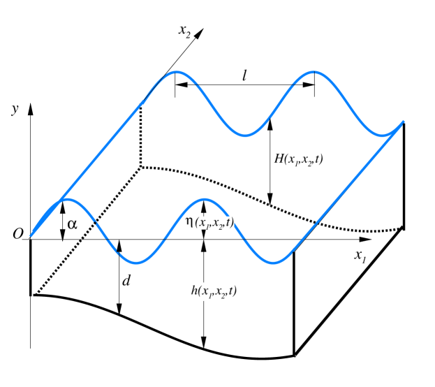
Figure 1. Sketch of the fluid domain.

The flow is considered to be completely determined if we find the velocity field $\boldsymbol{U}(\boldsymbol{x},\,y,\,t)\ =\ \bigl{(}\boldsymbol{u}(\boldsymbol{x},\,y,\,t),\,v(\boldsymbol{x},\,y,\,t)\bigr{)}$ ($\boldsymbol{u}=(u_{1},\,u_{2})$ being the horizontal velocity components) along with the pressure field $p(\boldsymbol{x},\,y,\,t)$ and the free surface elevation $\eta(\boldsymbol{x},\,t)$, which satisfy the system of Euler equations:

$$\boldsymbol{\nabla}\boldsymbol{\cdot}\boldsymbol{u}\ +\ v_{y}\ =\ 0\,,$$ (2.1)

$$\boldsymbol{u}_{t}\ +\ (\boldsymbol{u}\boldsymbol{\cdot}\boldsymbol{\nabla})\boldsymbol{u}\ +\ v\,\boldsymbol{u}_{y}\ +\ \boldsymbol{\nabla}p\ =\ 0\,,$$ (2.2)

$$v_{t}\ +\ \boldsymbol{u}\boldsymbol{\cdot}\boldsymbol{\nabla}v\ +\ v\,v_{y}\ +\ p_{y}\ =\ -g\,,$$ (2.3)

where $\boldsymbol{\nabla}\ =\ (\partial_{x_{1}},\,\partial_{x_{2}})$ denotes the horizontal gradient operator. The Euler equations are completed with free surface kinematic and dynamic boundary conditions

$$\eta_{t}\ +\ \boldsymbol{u}\boldsymbol{\cdot}\boldsymbol{\nabla}\eta\ =\ v\,,\quad y\ =\ \eta(\boldsymbol{x},\,t)\,,$$ (2.4)

$$p\ =\ 0\,,\quad y\ =\ \eta(\boldsymbol{x},\,t)\,.$$ (2.5)

Finally, on the bottom we impose the impermeability condition (i.e.  the fluid particles cannot penetrate the solid boundary), which states that the normal velocity on the bottom vanishes:

$$h_{t}\ +\ \boldsymbol{u}\boldsymbol{\cdot}\boldsymbol{\nabla}h\ +\ v\ =\ 0\,,\quad y\ =\ -h(\boldsymbol{x},\,t)\,.$$ (2.6)

Below we shall discuss also the components of the vorticity vector $\boldsymbol{\omega}\ =\ \boldsymbol{\nabla}\boldsymbol{\times}\ \boldsymbol{U}$, which are given by

$$\omega_{1}\ =\ v_{x_{2}}\ -\ u_{2,\,y}\,,$$

$$\omega_{2}\ =\ -v_{x_{1}}\ +\ u_{1,\,y}\,,$$

$$\omega_{3}\ =\ u_{2,\,x_{1}}\ -\ u_{1,\,x_{2}}\,.$$

Dimensionless variables

In order to study the propagation of long gravity waves, we have to scale the governing equations (2.1)–(2.3) along with the boundary conditions (2.4)–(2.6). For this purpose we choose characteristic scales of the flow. Let $\ell$, $d$ and $\upalpha$ be the typical (wave or basin) length, water depth and wave amplitude correspondingly (they are depicted in Figure 1). Then, dimensionless independent variables can be introduced as follows

$$x_{1,2}^{\ast}\ =\ \frac{x_{1,2}}{\ell}\,,\quad y^{\ast}\ =\ \frac{y}{d}\,,\^{A}~\quad t^{\ast}\ =\ \frac{t}{\ell/\sqrt{gd}}\,.$$

The dependent variables are scaled as

$$h^{\ast}\ =\ \frac{h}{d}\,,\quad\eta^{\ast}\ =\ \frac{\eta}{\upalpha}\,,\quad p^{\ast}\ =\ \frac{p}{(\rho)gd}\,,\quad\boldsymbol{u}^{\ast}\ =\ \frac{\boldsymbol{u}}{\sqrt{gd}}\,,\quad v^{\ast}\ =\ \frac{v}{d\sqrt{gd}/\ell}\,.$$

The components of vorticity $\boldsymbol{\omega}$ are scaled as

$$\omega_{1,2}^{\ast}\ =\ \frac{\omega_{1,2}}{\sqrt{gd}/d}\,,\qquad\omega_{3}^{\ast}\ =\ \frac{\omega_{3}}{\sqrt{gd}/\ell}\,.$$

The scaled version of the Euler equations (2.1)–(2.3) read now

$$\boldsymbol{\nabla}\boldsymbol{\cdot}\boldsymbol{u}\ +\ v_{y}\ =\ 0\,,$$ (2.7)

$$\boldsymbol{u}_{t}\ +\ (\boldsymbol{u}\boldsymbol{\cdot}\boldsymbol{\nabla})\boldsymbol{u}\ +\ v\,\boldsymbol{u}_{y}\ +\ \boldsymbol{\nabla}p\ =\ 0\,,$$ (2.8)

$$\mu^{2}\,\bigl{(}v_{t}\ +\ \boldsymbol{u}\boldsymbol{\cdot}\boldsymbol{\nabla}v\ +\ v\,v_{y}\bigr{)}\ +\ p_{y}\ =\ -1\,,$$ (2.9)

where we drop the asterisk symbol $\,\ast\,$ for the sake of notation compactness. Boundary conditions at the free surface similarly become

$$\varepsilon\,\bigl{(}\eta_{t}\ +\ \boldsymbol{u}\boldsymbol{\cdot}\boldsymbol{\nabla}\eta\bigr{)}\ =\ v\,,\quad y\ =\ \varepsilon\,\eta(\boldsymbol{x},\,t)\,,$$ (2.10)

$$p\ =\ 0\,,\quad y\ =\ \varepsilon\,\eta(\boldsymbol{x},\,t)\,.$$ (2.11)

It can be easily checked that the bottom boundary condition (2.6) remains invariant under this scaling. Finally, the scaled components of vorticity $\omega^{\ast}$ are

$$\omega_{1}\ =\ \mu^{2}\,v_{x_{2}}\ -\ u_{2,\,y}\,,$$

$$\omega_{2}\ =\ -\mu^{2}\,v_{x_{1}}\ +\ u_{1,\,y}\,,$$

$$\omega_{3}\ =\ u_{2,\,x_{1}}\ -\ u_{1,\,x_{2}}\,.$$

Above we introduced two important dimensionless parameters:

Nonlinearity:

$\varepsilon\ \mathop{\stackrel{{\scriptstyle\mathrm{def}}}{{:=}}}\ \dfrac{\upalpha}{d}$, which measures the deviation of waves with respect to the unperturbed water level

Dispersion:

$\mu\ \mathop{\stackrel{{\scriptstyle\mathrm{def}}}{{:=}}}\ \dfrac{d}{\ell}$, which indicates how long the waves are comparing to the mean depth (or equivalently how shallow is the water)

Long wave approximation

In approximate shallow water systems the dynamic variables are the total water depth $\mathcal{H}(\boldsymbol{x},\,t)\ \mathop{\stackrel{{\scriptstyle\mathrm{def}}}{{:=}}}\ h(\boldsymbol{x},\,t)\ +\ \varepsilon\,\eta(\boldsymbol{x},\,t)$ and some vector $\bar{\boldsymbol{u}}(\boldsymbol{x},\,t)$ which is supposed to approximate the horizontal velocity vector of the full model $\boldsymbol{u}(\boldsymbol{x},\,y,\,t)$. In many works $\bar{\boldsymbol{u}}(\boldsymbol{x},\,t)$ is chosen as the trace of the horizontal velocity $\boldsymbol{u}$ at certain surface $y\ =\ \mathcal{Y}_{\sigma}(\boldsymbol{x},\,t)$ in the fluid bulk [63, 42, 54], i.e.

$$\bar{\boldsymbol{u}}(\boldsymbol{x},\,t)\ \mathop{\stackrel{{\scriptstyle\mathrm{def}}}{{:=}}}\ \boldsymbol{u}\bigl{(}\boldsymbol{x},\,\mathcal{Y}_{\sigma}(\boldsymbol{x},\,t),\,t\bigr{)}\,.$$ (2.12)

Another popular choice for the velocity variable consists in taking the depth-averaged velocity [69, 66, 68, 24, 28]:

$$\bar{\boldsymbol{u}}(\boldsymbol{x},\,t)\ \mathop{\stackrel{{\scriptstyle\mathrm{def}}}{{:=}}}\ \frac{1}{\mathcal{H}(\boldsymbol{x},\,t)}\;\int_{-h(\boldsymbol{x},\,t)}^{\;\varepsilon\,\eta(\boldsymbol{x},\,t)}\,\boldsymbol{u}(\boldsymbol{x},\,y,\,t)\;\mathrm{d}y\,.$$ (2.13)

By applying the mean value theorem [79] to the last integral, we obtain that two approaches are mathematically formally equivalent:

$$\bar{\boldsymbol{u}}(\boldsymbol{x},\,t)\ \equiv\ \boldsymbol{u}\bigl{(}\boldsymbol{x},\,\mathcal{Y}_{\xi}(\boldsymbol{x},\,t),\,t\bigr{)}\,.$$

However, this time the surface $y\ =\ \mathcal{Y}_{\xi}(\boldsymbol{x},\,t)$ remains unknown, while above it was explicitly specified. We only know that such surface exists.

Below we shall consider only long wave approximation to the full Euler equations. Namely, we assume that $\bar{\boldsymbol{u}}(\boldsymbol{x},\,t)$ approximates the true horizontal velocity $\boldsymbol{u}(\boldsymbol{x},\,y,\,t)$ to the order $\mathcal{O}(\mu^{2})$, i.e.

$$\boldsymbol{u}(\boldsymbol{x},\,y,\,t)\ =\ \bar{\boldsymbol{u}}(\boldsymbol{x},\,t)\ +\ \mu^{2}\,\tilde{\boldsymbol{u}}(\boldsymbol{x},\,y,\,t)\,.$$ (2.14)

By integrating the continuity equation (2.7) over the total depth and taking into account boundary conditions (2.6), (2.10) we obtain the mass conservation equation

$$\mathcal{H}_{t}\ +\ \boldsymbol{\nabla}\boldsymbol{\cdot}(\mathcal{H}\,\bar{\boldsymbol{u}})\ =\ -\mu^{2}\,\boldsymbol{\nabla}\boldsymbol{\cdot}(\mathcal{H}\mathscr{U})\,,$$ (2.15)

where

$$\mathscr{U}(\boldsymbol{x},\,t)\ \mathop{\stackrel{{\scriptstyle\mathrm{def}}}{{:=}}}\ \frac{1}{\mathcal{H}(\boldsymbol{x},\,t)}\,\int_{-h(\boldsymbol{x},\,t)}^{\;\varepsilon\eta\,(\boldsymbol{x},\,t)}\,\tilde{\boldsymbol{u}}(\boldsymbol{x},\,y,\,t)\;\mathrm{d}y\,.$$ (2.16)

If we choose the variable $\bar{\boldsymbol{u}}$ to be depth-averaged, then $\mathscr{U}(\boldsymbol{x},\,t)\ \equiv\ 0$ and the mass conservation equation (2.15) takes the very familiar form

$$\mathcal{H}_{t}\ +\ \boldsymbol{\nabla}\boldsymbol{\cdot}(\mathcal{H}\bar{\boldsymbol{u}})\ =\ 0\,.$$

Integration of equation (2.7) over the vertical coordinate in the limits from $-h(\boldsymbol{x},\,t)$ to $y$ and taking into account the bottom boundary condition (2.6) leads to the following representation for the vertical velocity in the fluid column:

$$v(\boldsymbol{x},\,y,\,t)\ =\ -\mathscrbf{D}h\ -\ (y+h)\boldsymbol{\nabla}\boldsymbol{\cdot}\bar{\boldsymbol{u}}\ +\ \mathcal{O}(\mu^{2})\,,$$ (2.17)

where for the sake of simplicity we introduced the material (or total, or convective) derivative operator:

$$\mathscrbf{D}\,[\,\cdot\,]\ \mathop{\stackrel{{\scriptstyle\mathrm{def}}}{{:=}}}\ [\,\cdot\,]_{\,t}\ +\ \bar{\boldsymbol{u}}\boldsymbol{\cdot}\boldsymbol{\nabla}\;[\,\cdot\,]\,.$$

Below the powers of this operator will appear in our computations:

$$\mathscrbf{D}^{k}\,[\,\cdot\,]\ \mathop{\stackrel{{\scriptstyle\mathrm{def}}}{{:=}}}\ \underbrace{\mathscrbf{D}\cdot\mathscrbf{D}\cdot\ldots\cdot\mathscrbf{D}}_{k\mbox{ times}}\;[\,\cdot\,]\,,\qquad k\ \geqslant\ 1\,.$$

We have to express asymptotically also the pressure field $p(\boldsymbol{x},\,y,\,t)$ in terms of the dynamic variables $\bigl{(}\mathcal{H}(\boldsymbol{x},\,t),\,\bar{\boldsymbol{u}}(\boldsymbol{x},\,t)\bigr{)}$. Thus, we integrate the vertical momentum equation (2.9) over the vertical coordinate in the limits from $y$ to the free surface:

$$p(\boldsymbol{x},\,y,\,t)\ =\ \mu^{2}\,\int_{y}^{\;\varepsilon\eta(\boldsymbol{x},\,t)}\Bigl{[}\,\mathscrbf{D}\,v\ +\ v\,v_{y}\ +\ \mathcal{O}(\mu^{2})\,\Bigr{]}\;\mathrm{d}y\ -\ y\ +\ \varepsilon\,\eta(\boldsymbol{x},\,t)\,.$$ (2.18)

The integrand can be expressed in term of $\mathcal{H}(\boldsymbol{x},\,t)$ and $\bar{\boldsymbol{u}}(\boldsymbol{x},\,t)$ using representation (2.17):

$$\mathscrbf{D}\,v\ +\ v\,v_{y}\ =\ -(y+h)\,\mathscr{R}_{1}\ -\ \mathscr{R}_{2}\ +\ \mathcal{O}(\mu^{2})\,,$$

where we defined

$$\mathscr{R}_{1}(\boldsymbol{x},\,t)\ \mathop{\stackrel{{\scriptstyle\mathrm{def}}}{{:=}}}\ \mathscrbf{D}\,\boldsymbol{\nabla}\boldsymbol{\cdot}\bar{\boldsymbol{u}}\ -\ (\boldsymbol{\nabla}\boldsymbol{\cdot}\bar{\boldsymbol{u}})^{2}\,,$$

$$\mathscr{R}_{2}(\boldsymbol{x},\,t)\ \mathop{\stackrel{{\scriptstyle\mathrm{def}}}{{:=}}}\ \mathscrbf{D}^{2}h\,.$$

Substituting the last result into the integral representation (2.18) and integrating it exactly in $y$ leads the following expression of the pressure field in the fluid layer:

$$p\ =\ \mathcal{H}\ -\ (y+h)\ -\ \mu^{2}\,\biggl{[}\,\bigl{(}\mathcal{H}\ -\ (y+h)\bigr{)}\,\mathscr{R}_{2}\ +\ \Bigl{(}\frac{\mathcal{H}^{\,2}}{2}\ -\ \frac{(y+h)^{2}}{2}\Bigr{)}\,\mathscr{R}_{1}\,\biggr{]}\ +\ \mathcal{O}(\mu^{4})\,.$$ (2.19)

Notice that this representation does not depend on the expression of the velocity correction $\tilde{\boldsymbol{u}}(\boldsymbol{x},\,t)$. If in the last formula we neglect terms of $\mathcal{O}(\mu^{4})$ and return to physical variables, we can obtain the pressure reconstruction formula in the fluid bulk:

$$\frac{p}{\rho}\ =\ g\,\Bigl{[}\,\mathcal{H}\ -\ (y+h)\,\Bigr{]}\ -\ \biggl{[}\,\bigl{(}\mathcal{H}\ -\ (y+h)\bigr{)}\,\mathscr{R}_{2}\ +\ \Bigl{(}\frac{\mathcal{H}^{\,2}}{2}\ -\ \frac{(y+h)^{2}}{2}\Bigr{)}\,\mathscr{R}_{1}\,\biggr{]}\,.$$

We underline the fact that the last formula is accurate to the order $\mathcal{O}(\mu^{4})$. This formula will be used in [45] in order to reconstruct the pressure field under a solitary wave, which undergoes some nonlinear transformations.

In order to obtain an evolution equation for the approximate horizontal velocity $\bar{\boldsymbol{u}}(\boldsymbol{x},\,t)$ we integrate over the vertical coordinate equation (2.8):

$$\int_{-h}^{\;\varepsilon\eta}\bigl{[}\,\boldsymbol{u}_{t}\ +\ (\boldsymbol{u}\boldsymbol{\cdot}\boldsymbol{\nabla})\boldsymbol{u}\ +\ v\,\boldsymbol{u}_{y}\,\bigr{]}\;\mathrm{d}y\ +\ \boldsymbol{\nabla}\int_{-h}^{\;\varepsilon\eta}p\;\mathrm{d}y\ -\ \left.p\right|_{y=-h}\cdot\boldsymbol{\nabla}h\ =\ 0\,.$$ (2.20)

The pressure variable can be easily eliminated from the last equation using the representation formula (2.19):

$$\boldsymbol{\nabla}\int_{-h}^{\;\varepsilon\eta}p\;\mathrm{d}y\ -\ \left.p\right|_{y=-h}\cdot\boldsymbol{\nabla}h\ =\\ =\ \varepsilon\,\mathcal{H}\boldsymbol{\nabla}h\ -\ \mu^{2}\Bigl{[}\,\boldsymbol{\nabla}\bigl{(}{\textstyle{1\over 3}}\mathcal{H}^{\,3}\mathscr{R}_{1}\ +\ {\textstyle{1\over 2}}\mathcal{H}^{\,2}\mathscr{R}_{2}\bigr{)}\ -\ \mathcal{H}\,\boldsymbol{\nabla}h\,\bigl{(}{\textstyle{1\over 2}}\mathcal{H}\mathscr{R}_{1}\ +\ \mathscr{R}_{2}\bigr{)}\,\Bigr{]}\ +\ \mathcal{O}(\mu^{4})\,.$$

Then, using the representation (2.17) for the vertical velocity $v$, we can write

$$\int_{-h}^{\;\varepsilon\eta}v\,\boldsymbol{u}_{y}\;\mathrm{d}y\ =\ -\mu^{2}\int_{-h}^{\;\varepsilon\eta}\bigl{[}\,\mathscrbf{D}h\ +\ (y+h)\boldsymbol{\nabla}\boldsymbol{\cdot}\bar{\boldsymbol{u}}\,\bigr{]}\,\tilde{\boldsymbol{u}}_{y}\;\mathrm{d}y\ +\ \mathcal{O}(\mu^{4})$$

$$=\ -\left.\mu^{2}(\mathscrbf{D}h)\cdot\tilde{\boldsymbol{u}}\right|_{y\,=\,-h}^{y\,=\,\varepsilon\eta}\ -\ \mu^{2}\,\boldsymbol{\nabla}\boldsymbol{\cdot}\bar{\boldsymbol{u}}\underbrace{\int_{-h}^{\;\varepsilon\eta}(y+h)\tilde{\boldsymbol{u}}_{y}\;\mathrm{d}y}_{(\ast)}\ +\ \mathcal{O}(\mu^{4})\,.$$

The integral ($\ast$) can be computed using integration by parts

$$\int_{-h}^{\;\varepsilon\eta}(y+h)\,\tilde{\boldsymbol{u}}_{y}\;\mathrm{d}y\ =\ \left.\mathcal{H}\cdot\tilde{\boldsymbol{u}}\right|^{y\,=\,\varepsilon\eta}\ -\ \mathcal{H}\mathscr{U}\,.$$

Combining together these results, we obtain the following asymptotic formula

$$\frac{1}{\mu^{2}}\int_{-h}^{\;\varepsilon\eta}v\,\boldsymbol{u}_{y}\;\mathrm{d}y\ =\ \left.(\mathscrbf{D}h)\cdot\tilde{\boldsymbol{u}}\right|_{y\,=\,-h}\ -\ \bigl{[}\,\mathscrbf{D}h\ +\ \mathcal{H}\,\boldsymbol{\nabla}\boldsymbol{\cdot}\bar{\boldsymbol{u}}\,\bigr{]}\left.\tilde{\boldsymbol{u}}\right|^{y\,=\,\varepsilon\eta}\ +\ \mathcal{H}\mathscr{U}\boldsymbol{\nabla}\boldsymbol{\cdot}\bar{\boldsymbol{u}}\ +\ \mathcal{O}(\mu^{2})\,.$$

Finally, we take care of convective terms

$$\int_{-h}^{\;\varepsilon\eta}\bigl{[}\,\boldsymbol{u}_{t}\ +\ (\boldsymbol{u}\boldsymbol{\cdot}\boldsymbol{\nabla})\boldsymbol{u}\,\bigr{]}\;\mathrm{d}y\ =\ \int_{-h}^{\;\varepsilon\eta}\mathscrbf{D}\bar{\boldsymbol{u}}\;\mathrm{d}y\ +\ \mu^{2}\int_{-h}^{\;\varepsilon\eta}\mathscrbf{D}\tilde{\boldsymbol{u}}\;\mathrm{d}y\ +\ \mu^{2}\int_{-h}^{\;\varepsilon\eta}(\tilde{\boldsymbol{u}}\boldsymbol{\cdot}\boldsymbol{\nabla})\bar{\boldsymbol{u}}\;\mathrm{d}y\ +\ \mathcal{O}(\mu^{4})\\ =\ \mathcal{H}\mathscrbf{D}\bar{\boldsymbol{u}}\ +\ \mu^{2}\Bigl{[}\,\mathscrbf{D}\bigl{[}\,\mathcal{H}\mathscr{U}\,\bigr{]}\ -\ \mathscrbf{D}[\,\varepsilon\eta\,]\cdot\left.\tilde{\boldsymbol{u}}\right|^{y\,=\,\varepsilon\,\eta}\ -\ \mathscrbf{D}h\cdot\left.\tilde{\boldsymbol{u}}\right|_{y\,=\,-h}\ +\ \mathcal{H}(\mathscr{U}\boldsymbol{\cdot}\boldsymbol{\nabla})\,\bar{\boldsymbol{u}}\,\Bigr{]}\ +\ \mathcal{O}(\mu^{4})\,.$$

Finally, we obtain

$$\int_{-h}^{\;\varepsilon\eta}\bigl{[}\,\boldsymbol{u}_{t}\ +\ (\boldsymbol{u}\boldsymbol{\cdot}\boldsymbol{\nabla})\boldsymbol{u}\ +\ v\,\boldsymbol{u}_{y}\,\bigr{]}\;\mathrm{d}y\ =\ \mathcal{H}\mathscrbf{D}\bar{\boldsymbol{u}}\ -\ \mu^{2}\underbrace{\bigl{[}\,\mathscrbf{D}\mathcal{H}\ +\ \mathcal{H}\boldsymbol{\nabla}\boldsymbol{\cdot}\bar{\boldsymbol{u}}\,\bigr{]}}_{(\ast\ast)}\cdot\left.\tilde{\boldsymbol{u}}\right|^{y\,=\,\varepsilon\eta}\ +\\ +\ \mu^{2}\,\Bigl{[}\,\mathscrbf{D}\bigl{[}\,\mathcal{H}\mathscr{U}\,\bigr{]}\ +\ \mathcal{H}(\mathscr{U}\boldsymbol{\cdot}\boldsymbol{\nabla})\,\bar{\boldsymbol{u}}\ +\ \mathcal{H}\mathscr{U}\boldsymbol{\nabla}\boldsymbol{\cdot}\bar{\boldsymbol{u}}\,\Bigr{]}\,.$$

From the mass conservation equation (2.15) we have

$$\mathscrbf{D}\mathcal{H}\ +\ \mathcal{H}\,\boldsymbol{\nabla}\boldsymbol{\cdot}\bar{\boldsymbol{u}}\ =\ -\mu^{2}\,\boldsymbol{\nabla}\boldsymbol{\cdot}(\mathcal{H}\mathscr{U})\ =\ \mathcal{O}(\mu^{2})\,.$$

Thus, the term ($\ast\ast$) can be asymptotically neglected. As a result we have

$$\int_{-h}^{\;\varepsilon\eta}\bigl{[}\,\boldsymbol{u}_{t}\ +\ (\boldsymbol{u}\boldsymbol{\cdot}\boldsymbol{\nabla})\boldsymbol{u}\ +\ v\,\boldsymbol{u}_{y}\,\bigr{]}\;\mathrm{d}y\ =\ \mathcal{H}\mathscrbf{D}\bar{\boldsymbol{u}}\ +\ \mu^{2}\,\Bigl{[}\,\mathscrbf{D}\bigl{[}\,\mathcal{H}\mathscr{U}\,\bigr{]}\ +\ \mathcal{H}(\mathscr{U}\boldsymbol{\cdot}\boldsymbol{\nabla})\,\bar{\boldsymbol{u}}\ +\ \mathcal{H}\mathscr{U}\boldsymbol{\nabla}\boldsymbol{\cdot}\bar{\boldsymbol{u}}\,\Bigr{]}\ +\ \mathcal{O}(\mu^{4})\,.$$

Substituting all these intermediate results into depth-integrated horizontal momentum equation (2.20), we obtain the required evolution equation for $\bar{\boldsymbol{u}}$:

$$\bar{\boldsymbol{u}}_{t}\ +\ (\bar{\boldsymbol{u}}\boldsymbol{\cdot}\boldsymbol{\nabla})\bar{\boldsymbol{u}}\ +\ \varepsilon\,\boldsymbol{\nabla}\eta\ =\ \frac{\mu^{2}}{\mathcal{H}}\;\Bigl{[}\,\boldsymbol{\nabla}\bigl{(}{\textstyle{1\over 3}}\mathcal{H}^{\,3}\mathscr{R}_{1}\ +\ {\textstyle{1\over 2}}\mathcal{H}^{\,2}\mathscr{R}_{2}\bigr{)}\ -\ \mathcal{H}\,\boldsymbol{\nabla}h\,\bigl{(}{\textstyle{1\over 2}}\mathcal{H}\mathscr{R}_{1}\ +\ \mathscr{R}_{2}\bigr{)}\,\Bigr{]}\\ -\ \frac{\mu^{2}}{\mathcal{H}}\;\Bigl{[}\,\mathscrbf{D}\bigl{[}\,\mathcal{H}\mathscr{U}\,\bigr{]}\ +\ \mathcal{H}(\mathscr{U}\boldsymbol{\cdot}\boldsymbol{\nabla})\,\bar{\boldsymbol{u}}\ +\ \mathcal{H}\mathscr{U}\boldsymbol{\nabla}\boldsymbol{\cdot}\bar{\boldsymbol{u}}\,\Bigr{]}\,.$$ (2.21)

The last equation may look complicated. However, it can be rewritten in a clearer way by pointing out explicitly the non-hydrostatic pressure effects. It turns out that it is advantageous to introduce the depth-integrated (but not depth-averaged) pressure:

$$\mathscr{P}(\mathcal{H},\,\bar{\boldsymbol{u}})\ \mathop{\stackrel{{\scriptstyle\mathrm{def}}}{{:=}}}\ \int_{-h}^{\;\varepsilon\eta}\,p\;\mathrm{d}y\ =\ \frac{\mathcal{H}^{\,2}}{2}\ -\ \mu^{2}\,\Bigl{(}{\textstyle{1\over 3}}\mathcal{H}^{\,3}\mathscr{R}_{1}\ +\ {\textstyle{1\over 2}}\mathcal{H}^{\,2}\mathscr{R}_{2}\Bigr{)}\,.$$ (2.22)

We introduce also the pressure trace $\check{p}$ at the bottom:

$$\check{p}(x,\,t)\ \mathop{\stackrel{{\scriptstyle\mathrm{def}}}{{:=}}}\ \left.p\right|_{y\,=\,-h}\ =\ \mathcal{H}\ -\ \mu^{2}\,\Bigl{(}{\textstyle{1\over 2}}\mathcal{H}^{\,2}\mathscr{R}_{1}\ +\ \mathcal{H}\mathscr{R}_{2}\Bigr{)}\,.$$

Using these new variables equation (2.21) becomes

$$\bar{\boldsymbol{u}}_{t}\ +\ (\bar{\boldsymbol{u}}\boldsymbol{\cdot}\boldsymbol{\nabla})\bar{\boldsymbol{u}}\ +\ \frac{\boldsymbol{\nabla}\mathscr{P}}{\mathcal{H}}\ =\ \frac{\check{p}\,\boldsymbol{\nabla}h}{\mathcal{H}}\ -\ \frac{\mu^{2}}{\mathcal{H}}\;\Bigl{[}\,(\mathcal{H}\mathscr{U})_{t}\ +\ (\bar{\boldsymbol{u}}\boldsymbol{\cdot}\boldsymbol{\nabla})(\mathcal{H}\mathscr{U})\ +\ \mathcal{H}(\mathscr{U}\boldsymbol{\cdot}\boldsymbol{\nabla})\,\bar{\boldsymbol{u}}\ +\ \mathcal{H}\mathscr{U}\boldsymbol{\nabla}\boldsymbol{\cdot}\bar{\boldsymbol{u}}\,\Bigr{]}\,.$$

The derived system of equations admits an elegant conservative form:

$$\mathcal{H}_{t}\ +\ \boldsymbol{\nabla}\boldsymbol{\cdot}[\,\mathcal{H}\boldsymbol{U}\,]\ =\ 0\,,$$ (2.23)

$$(\mathcal{H}\,\boldsymbol{U})_{t}\ +\ \boldsymbol{\nabla}\boldsymbol{\cdot}\Bigl{[}\,\mathcal{H}\bar{\boldsymbol{u}}\boldsymbol{\otimes}\boldsymbol{U}\ +\ \mathscr{P}(\mathcal{H},\,\bar{\boldsymbol{u}})\cdot\mathbb{I}\ +\ \mu^{2}\mathcal{H}\,\mathscr{U}\boldsymbol{\otimes}\bar{\boldsymbol{u}}\,\Bigr{]}\ =\ \check{p}\,\boldsymbol{\nabla}h\,,$$ (2.24)

where we introduced a new velocity variable $\boldsymbol{U}\ \mathop{\stackrel{{\scriptstyle\mathrm{def}}}{{:=}}}\ \bar{\boldsymbol{u}}\ +\ \mu^{2}\,\mathscr{U}$ and $\mathbb{I}\ \in\ \mathrm{Mat}\,_{2\,\times\,2}(\mathds{R})$ is the identity matrix. Operator $\boldsymbol{\otimes}$ is the tensorial product, i.e.  for two vectors $\boldsymbol{u}\ \in\ \mathds{R}^{m}$ and $\boldsymbol{v}\ \in\ \mathds{R}^{n}$

$$\boldsymbol{u}\boldsymbol{\otimes}\boldsymbol{v}\ \mathop{\stackrel{{\scriptstyle\mathrm{def}}}{{:=}}}\ (u_{i}\cdot v_{j})^{1\,\leqslant\,i\,\leqslant\ m}_{1\,\leqslant\,j\,\leqslant\,n}\ \in\ \mathrm{Mat}\,_{m\,\times\,n}(\mathds{R})\,.$$

From now on equations (2.23), (2.24) will be referred to as the base model of our study. In order to close the last system of equations (2.23), (2.24), we have to express the variable $\mathscr{U}$ in terms of other dynamic variables $\mathcal{H}(\boldsymbol{x},\,t)$ and $\bar{\boldsymbol{u}}(\boldsymbol{x},\,t)$. Several popular choices will be discussed below. Notice also that nowhere in the derivation above the flow irrotationality was assumed.

Remark 1.

Notice that taking formally the limit $\mu\ \to\ 0$ in equations (2.23), (2.24) yields straightforwardly the well-known Nonlinear Shallow Water (NSW or Saint-Venant) Equations [23]. Thus, our base model satisfies the Bohr correspondence principle. This property is crucial for robust physical wave modelling in coastal environments. Indeed, a wave approaching continental shelf undergoes nonlinear transformations: the water depth is decreasing and the wave amplitude grows, which often leads to the formation of undular bores. The model has to follow these transformations. Mathematically it means that the model equations should encompass a range of physical regimes varying from fairly shallow water to intermediate depths [38]. There exists an option of coupling different hydrodynamic models as it was done e.g. in [53]. However, the coupling represents a certain number of difficulties, e.g.

• Boundary conditions at artificial interfaces?

• How to determine automatically the physical regime?

• Dynamic evolution and handling of model applicability areas…

Consequently, in this study we let the physical model to do this work for us.

2.2.1  Energy conservation

We would like to raise the question of energy conservation in nonlinear dispersive wave models. The full Euler equations naturally have this property. So, it is a priori natural to require that a good approximation to Euler equations conserves the energy as well [36]. An energy conservation equation can be established for the base model (2.23), (2.24) for some choices of the variable $\mathscr{U}(\mathcal{H},\,\bar{\boldsymbol{u}})$. For instance, the classical SGN model discussed in the following section enjoys this property (it corresponds to the choice $\mathscr{U}\ \equiv\ \boldsymbol{0}$). On moving bottoms this property was discussed in [36]. Here we provide only the final result, i.e. the total energy equation for SGN model on a general moving bottom:

$$(\mathcal{H}\,\mathscr{E})_{t}\ +\ \boldsymbol{\nabla}\boldsymbol{\cdot}\Bigl{[}\,\mathcal{H}\bar{\boldsymbol{u}}\,\Bigl{(}\mathscr{E}\ +\ \frac{\mathscr{P}}{\mathcal{H}}\Bigr{)}\,\Bigr{]}\ =\ -\check{p}\,h_{t}\,,$$

where the total energy $\mathscr{E}$ is defined as

$$\mathscr{E}\ \mathop{\stackrel{{\scriptstyle\mathrm{def}}}{{:=}}}\ {\textstyle{1\over 2}}\,\lvert\,\bar{\boldsymbol{u}}\,\rvert^{2}\ +\ {\textstyle{1\over 6}}\,\mathcal{H}^{\,2}\,(\boldsymbol{\nabla}\boldsymbol{\cdot}\bar{\boldsymbol{u}})^{2}\ +\ {\textstyle{1\over 2}}\,\mathcal{H}\,(\mathscrbf{D}h)\,(\boldsymbol{\nabla}\boldsymbol{\cdot}\bar{\boldsymbol{u}})\ +\ {\textstyle{1\over 2}}\,(\mathscrbf{D}h)^{2}\ +\ \frac{g}{2}\;(\mathcal{H}\ -\ 2h)\,.$$

For other choices of the closure $\mathscr{U}(\mathcal{H},\,\bar{\boldsymbol{u}})$ this question of energy conservation has to be studied separately.

Remark 2.

Recently, Clamond, Dutykh & Mitsotakis (2015) [20] proposed a dispersion-improved SGN-type model which enjoys the energy conservation property. The method employed in that study is the variational approach: the preservation of the variational structure is crucial for the preservation of several invariants.

2.2.2  Galilean invariance

The same questions can be raised about the Galilean invariance property as well. This property is of fundamental importance for any mathematical model that provide a physically sound description of water waves (stemming from Classical Mechanics and Classical Physics). Some thoughts and tentative corrections can be found in [27, 30]. The base model (2.23), (2.24) is Galilean invariant under reasonable assumptions on the closure velocity vector $\mathscr{U}$.

Galilean invariance principle states that all mechanical laws are the same in any inertial frame of reference [49]. Consequently, the mathematical form of governing equations should be the same as well. It was proposed by Galileo Galilei in 1632 [37]. Consider the horizontal Galilean boost transformation between two inertial frames of reference:

$$\boldsymbol{x}^{\,\prime}\ =\ \boldsymbol{x}\ +\ \boldsymbol{\mathrm{C}}\,t\,,\qquad y^{\,\prime}\ =\ y\,,\qquad t^{\,\prime}\ =\ t\,,$$ (2.25)

where $\boldsymbol{\mathrm{C}}$ is a constant motion speed of the new coordinate system (with primes) relatively to the initial one (without primes). Notice that scalar quantities such as $\mathcal{H}(\boldsymbol{x},\,t)$ and $h(\boldsymbol{x},\,t)$ remain invariant since they are defined as distances between two points and distances are preserved by the Galilean transformation (2.25). Let us see how the horizontal velocity variable changes under the Galilean transformation:

$$\boldsymbol{u}(\boldsymbol{x},\,y,\,t)\ \mathop{\stackrel{{\scriptstyle\mathrm{def}}}{{:=}}}\ \frac{\mathrm{d}\boldsymbol{x}}{\mathrm{d}\/t}\ =\ \frac{\mathrm{d}\boldsymbol{x}^{\,\prime}}{\mathrm{d}\/t}\ -\ \boldsymbol{\mathrm{C}}\ \mathop{\stackrel{{\scriptstyle\mathrm{def}}}{{=:}}}\ \boldsymbol{u}^{\,\prime}(\boldsymbol{x}^{\,\prime},\,y^{\,\prime},\,t^{\,\prime})\ -\ \boldsymbol{\mathrm{C}}\,.$$

It is not difficult to understand that the same transformation rule applies to $\bar{\boldsymbol{u}}(\boldsymbol{x},\,t)$ regardless if it is defined as a trace or depth-averaged velocity:

$$\bar{\boldsymbol{u}}\ =\ \bar{\boldsymbol{u}}^{\,\prime}\ -\ \boldsymbol{\mathrm{C}}\,.$$

Indeed, the last claim is obvious for the case of the trace operator. Let us check it for the depth-averaging operator:

$$\bar{\boldsymbol{u}}(\boldsymbol{x},\,t)\ \mathop{\stackrel{{\scriptstyle\mathrm{def}}}{{:=}}}\ \frac{1}{\mathcal{H}}\,\int_{-h}^{\;\varepsilon\,\eta}\^{A}~\boldsymbol{u}\;\mathrm{d}y\ =\ \frac{1}{\mathcal{H}^{\,\prime}}\,\int_{-h^{\,\prime}}^{\;\varepsilon\,\eta^{\,\prime}}\^{A}~\bigl{(}\boldsymbol{u}^{\,\prime}\ -\ \boldsymbol{\mathrm{C}}\bigr{)}\;\mathrm{d}y^{\,\prime}\ =\\ =\ \frac{1}{\mathcal{H}^{\,\prime}}\,\int_{-h^{\,\prime}}^{\;\varepsilon\,\eta^{\,\prime}}\^{A}~\boldsymbol{u}^{\,\prime}\;\mathrm{d}y^{\,\prime}\ -\ \boldsymbol{\mathrm{C}}\ \mathop{\stackrel{{\scriptstyle\mathrm{def}}}{{=:}}}\ \bar{\boldsymbol{u}}^{\,\prime}(\boldsymbol{x}^{\,\prime},\,t^{\,\prime})\ -\ \boldsymbol{\mathrm{C}}\,.$$

If the velocity $\bar{\boldsymbol{u}}(\boldsymbol{x},\,t)$ is defined in a different way, its transformation rule has to be studied separately. From the definition (2.16) it follows that the velocity correction $\mathscr{U}$ should remain invariant under the Galilean boost (2.25) (since it is defined as a difference of two velocities):

$$\mathscr{U}^{\,\prime}\ \equiv\ \mathscr{U}\,.$$ (2.26)

In the following we shall assume that the chosen closure $\mathscr{U}(\mathcal{H},\,\bar{\boldsymbol{u}})$ satisfy the last transformation rule.

Finally, let us discuss the invariance of the base model (2.23), (2.24). Basically, this property follows from the transformation rule (2.26), from the fact that $\boldsymbol{\mathrm{C}}\ =\ \mathrm{const}$ and the following observation:

$$\mathscrbf{D}\mathcal{H}\ \equiv\ \mathscrbf{D}^{\,\prime}\mathcal{H}^{\,\prime}\,,\^{A}~\qquad\mathscrbf{D}\bar{\boldsymbol{u}}\ \equiv\ \mathscrbf{D}^{\,\prime}\bar{\boldsymbol{u}}^{\,\prime}\,.$$

The pressure variables $\mathscr{P}$ and $\check{p}$ remain invariant as well, since they depend on velocity through $\mathscr{R}_{1}$ and $\mathscr{R}_{2}$, which depend in their term only on the full derivative and divergence of the velocity $\bar{\boldsymbol{u}}$. Thus, the base model (2.23), (2.24) is Galilean invariant under not very restrictive assumptions made above.

Remark 3.

Many Boussinesq-type equations derived and published in the literature are not Galilean invariant. As a classical such example we can mention Peregrine’s (1967) system [66]. In [36] it was shown how to derive a weakly nonlinear model from the fully nonlinear one in such a way that the reduced Boussinesq-type model has the Galilean invariance and energy conservation properties.

Serre–Green–Naghdi equations

The celebrated Serre–Green–Naghdi (SGN) equations can be obtained by choosing the simplest possible closure, i.e.

$$\mathscr{U}\ \equiv\ \boldsymbol{0}\,.$$

This closure follows from the fact that the velocity variable $\bar{\boldsymbol{u}}$ chosen in SGN equations is precisely the depth-averaged velocity. Thus, $\tilde{\boldsymbol{u}}(\boldsymbol{x},\,t)\ \equiv\ \boldsymbol{0}$ and from (2.16) we have that $\mathscr{U}(\boldsymbol{x},\,t)\ \equiv\ \boldsymbol{0}$. By substituting the proposed closure into equations (2.23), (2.24), we obtain the SGN equations:

$$\mathcal{H}_{t}\ +\ \boldsymbol{\nabla}\boldsymbol{\cdot}[\,\mathcal{H}\bar{\boldsymbol{u}}\,]\ =\ 0\,,$$

$$(\mathcal{H}\bar{\boldsymbol{u}})_{t}\ +\ \boldsymbol{\nabla}\boldsymbol{\cdot}\Bigl{[}\,\mathcal{H}\bar{\boldsymbol{u}}\boldsymbol{\otimes}\bar{\boldsymbol{u}}\ +\ \mathscr{P}(\mathcal{H},\,\bar{\boldsymbol{u}})\cdot\mathbb{I}\,\Bigr{]}\ =\ \check{p}\,\boldsymbol{\nabla}h\,,$$

where $\mathscr{P}(\mathcal{H},\,\bar{\boldsymbol{u}})$ was defined in (2.22). The last equation can be written in a non-conservative form as well:

$$\bar{\boldsymbol{u}}_{t}\ +\ (\bar{\boldsymbol{u}}\boldsymbol{\cdot}\boldsymbol{\nabla})\bar{\boldsymbol{u}}\ +\ \frac{\boldsymbol{\nabla}\mathscr{P}}{\mathcal{H}}\ =\ \frac{\check{p}\,\boldsymbol{\nabla}h}{\mathcal{H}}\,.$$

The SGN equations have been rediscovered independently by a number of authors. The steady version of these equations can be already found in Rayleigh (1876) [52]. Then, this model in 1D was derived by Serre (1953) [69, 70] and by Su & Gardner (1969) [73]. A modern derivation was done by Green, Laws & Naghdi (1974) [39]. Later, in Soviet Union this system was derived also by Pelinovsky & Zheleznyak (1985) [78]. More recently, modern derivations of these equations based on variational principles have been proposed. Namely, Miles & Salmon (1985) [58] gave a derivation in Lagrangian (e.g. particle) description. The variational derivation in Eulerian description was given by Fedotova & Karepova (1996) [32] and later by Kim et al. (2001) [46] and Clamond & Dutykh (2012) [19]. Recently the multi-symplectic structure for SGN equations was proposed in [17].

Other particular cases

The scope of the present section is slightly broader than its title may suggest. More precisely, we consider the whole class of models where the velocity variable is defined on a certain surface inside the fluid, see equation (2.12) for the definition. We show in this section that the base model (2.23), (2.24) can be closed using the partial irrotationality condition. Namely, we assume that only two horizontal components of vorticity vanish, i.e.

$$\boldsymbol{u}_{y}\ =\ \mu^{2}\,\boldsymbol{\nabla}v\,.$$ (2.27)

Integration of this identity over $y$ and using representations (2.14), (2.17) leads

$$\tilde{\boldsymbol{u}}(\boldsymbol{x},\,y,\,t)\ =\ -(y+h)\,\bigl{[}\,\boldsymbol{\nabla}(\mathscrbf{D}h)\ +\ \boldsymbol{\nabla}h\,(\boldsymbol{\nabla}\boldsymbol{\cdot}\bar{\boldsymbol{u}})\,\bigr{]}\ -\ \frac{(y+h)^{2}}{2}\boldsymbol{\nabla}(\boldsymbol{\nabla}\boldsymbol{\cdot}\bar{\boldsymbol{u}})\ +\ \left.\tilde{\boldsymbol{u}}\right|_{y\,=\,-h}\ +\ \mathcal{O}(\mu^{2})\,.$$

Consequently, from (2.14) we obtain

$$\boldsymbol{u}(\boldsymbol{x},\,y,\,t)\ =\ \bar{\boldsymbol{u}}\ +\ \mu^{2}\,\Bigl{[}(y+h)\,\mathscr{A}\ +\ \frac{1}{2}\,(y+h)^{2}\,\mathscr{B}\ +\ \mathscr{C}\Bigr{]}\ +\ \mathcal{O}(\mu^{4})\,,$$ (2.28)

where we introduced for simplicity the following notation:

$$\mathscr{A}(\boldsymbol{x},\,t)\ \mathop{\stackrel{{\scriptstyle\mathrm{def}}}{{:=}}}\ -\boldsymbol{\nabla}(\mathscrbf{D}h)\ -\ \boldsymbol{\nabla}h\,(\boldsymbol{\nabla}\boldsymbol{\cdot}\bar{\boldsymbol{u}})\,,$$

$$\mathscr{B}(\boldsymbol{x},\,t)\ \mathop{\stackrel{{\scriptstyle\mathrm{def}}}{{:=}}}\ -\boldsymbol{\nabla}(\boldsymbol{\nabla}\boldsymbol{\cdot}\bar{\boldsymbol{u}})\,,$$

$$\mathscr{C}(\boldsymbol{x},\,t)\ \mathop{\stackrel{{\scriptstyle\mathrm{def}}}{{:=}}}\ \left.\tilde{\boldsymbol{u}}\right|_{y\,=\,-h}\,.$$

Let us evaluate both sides of equation (2.28) at $y_{\sigma}\ =\ \mathcal{Y}_{\sigma}(\boldsymbol{x},\,t)$. According to (2.12) we must have

$$\boldsymbol{u}\bigl{(}\boldsymbol{x},\,\mathcal{Y}_{\sigma}(\boldsymbol{x},\,t),\,t\bigr{)}\ \equiv\ \bar{\boldsymbol{u}}(\boldsymbol{x},\,t)\,.$$

Consequently, we have

$$\mathscr{C}(\boldsymbol{x},\,t)\ \equiv\ -(y_{\sigma}+h)\,\mathscr{A}\ -\ \frac{1}{2}\,(y_{\sigma}+h)^{2}\,\mathscr{B}\,.$$

Thus, coefficient $\mathscr{C}$ can be eliminated from (2.28) to give the following representation

$$\boldsymbol{u}(\boldsymbol{x},\,y,\,t)\ =\ \bar{\boldsymbol{u}}\ +\ \mu^{2}\,\Bigl{[}(y-y_{\sigma})\,\mathscr{A}\ +\ \frac{1}{2}\,\bigl{[}\,(y+h)^{2}\ -\ (y_{\sigma}+h)^{2}\,\bigr{]}\,\mathscr{B}\Bigr{]}\ +\ \mathcal{O}(\mu^{4})\,.$$

Substituting the last result into equation (2.16) yields the required closure relation:

$$\mathscr{U}(\mathcal{H},\,\bar{\boldsymbol{u}})\ =\ \Bigl{[}\,\frac{\mathcal{H}}{2}\ -\ (y_{\sigma}+h)\Bigr{]}\,\mathscr{A}\ +\ \Bigl{[}\frac{1}{6}\,\mathcal{H}^{\,2}\ -\ \frac{1}{2}\,(y_{\sigma}+h)^{2}\,\Bigr{]}\,\mathscr{B}\ +\ \mathcal{O}(\mu^{2})\,.$$ (2.29)

To summarize, under the assumption (2.27) that the first two components of the vorticity field vanish, we can propose a closure to the base model, after neglecting the terms of order $\mathcal{O}(\mu^{2})$ in (2.29).

Depth-averaged velocity.

It is interesting to obtain also the 3D velocity reconstruction formula in the case, where $\bar{\boldsymbol{u}}(\boldsymbol{x},\,t)$ is defined as the depth-averaged velocity (2.13). To do it, we average the equation (2.28) over the depth:

$$\frac{1}{\mathcal{H}}\;\int_{-h}^{\,\varepsilon\eta}\boldsymbol{u}(\boldsymbol{x},\,y,\,t)\;\mathrm{d}y\ =\ \bar{\boldsymbol{u}}(\boldsymbol{x},\,t)\ +\ \mu^{2}\,\Bigl{[}\,\frac{\mathcal{H}}{2}\;\mathscr{A}\ +\ \frac{\mathcal{H}^{\,2}}{6}\;\mathscr{B}\ +\ \mathscr{C}\,\Bigr{]}\ +\ \mathcal{O}(\mu^{2})\,.$$

Using the definition (2.13) of the depth-averaged velocity, we conclude that

$$\mathscr{C}\ =\ -\frac{\mathcal{H}}{2}\;\mathscr{A}\ -\ \frac{\mathcal{H}^{\,2}}{6}\;\mathscr{B}\ +\ \mathcal{O}(\mu^{2})\,.$$

By substituting the last expression into (2.28) we obtain the desired representation:

$$\boldsymbol{u}(\boldsymbol{x},\,y,\,t)\ =\ \bar{\boldsymbol{u}}(\boldsymbol{x},\,t)\ +\\ \mu^{2}\,\biggl{[}\,\Bigl{(}\frac{\mathcal{H}}{2}\ -\ y\ -\ h\Bigr{)}\cdot\Bigl{(}\boldsymbol{\nabla}\mathscrbf{D}h\ +\ (\boldsymbol{\nabla}\boldsymbol{\cdot}\bar{\boldsymbol{u}})\,\boldsymbol{\nabla}h\Bigr{)}\ +\ \Bigl{(}\frac{\mathcal{H}^{\,2}}{6}\ -\ \frac{(y+h)^{2}}{2}\Bigr{)}\,\boldsymbol{\nabla}(\boldsymbol{\nabla}\boldsymbol{\cdot}\bar{\boldsymbol{u}})\,\biggr{]}\ +\ \mathcal{O}(\mu^{4})\,.$$ (2.30)

The last formula will be used in [45] in order to reconstruct the 3D field under a propagating wave, which undergoes some nonlinear transformations. Formula (2.30) shows also that in shallow water flows the velocity distribution in the vertical coordinate $y$ is nearly quadratic.

Remark 4.

We underline that formula (2.30) is obtained under the assumption that the flow is irrotational. Without this assumption, in the most general case we can only use formula (2.14) by neglecting terms of the order $\mathcal{O}(\mu^{2})\,$. In other words, the velocity variable $\bar{\boldsymbol{u}}(\boldsymbol{x},\,t)$ approximates the 3D velocity field $\boldsymbol{u}(\boldsymbol{x},\,y,\,t)$ throughout the fluid to the order $\mathcal{O}(\mu^{2})\,$. However, in many applications this accuracy is not enough.

2.4.1  Lynett–Liu’s model

It can be shown that the base model (2.23), (2.24) supplemented by the proposed closure (2.29) is asymptotically equivalent to the well-known Lynett–Liu (2002) model derived in [54] under an additional assumption that the initial 3D flow is irrotational. This claim is true only up to the approximation order $\mathcal{O}(\mu^{4})$ and it can be checked by straightforward but tedious calculations.

Various choices of the level $y_{\sigma}$, where the horizontal velocity is defined, allow to obtain in a straightforward manner the fully nonlinear analogues of various existing models. Some of popular choices are discussed below.

2.4.2  Mei–Le Méhauté’s model

Consider the horizontal velocity variable defined at the bottom, i.e.

$$y_{\sigma}\ =\ -h(\boldsymbol{x},\,t)\,.$$

Substituting this value into (2.29) we obtain straightforwardly the following closure:

$$\mathscr{U}(\mathcal{H},\,\bar{\boldsymbol{u}})\ =\ \frac{1}{2}\,\mathcal{H}\,\mathscr{A}\ +\ \frac{1}{6}\,\mathcal{H}^{\,2}\,\mathscr{B}\ +\ \mathcal{O}(\mu^{2})\,.$$ (2.31)

In this way, the base model (2.23), (2.24) with the last closure becomes the celebrated Mei–Le Méhauté (1966) model [57].

2.4.3  Peregrine’s model and its generalizations

In 1967 Peregrine [66] considered a weakly nonlinear model with $y_{\sigma}\ =\ 0$. The fully nonlinear analogue of Peregrine’s model can be obtained if we take

$$y_{\sigma}\ =\ \varepsilon\,\eta\,(\boldsymbol{x},\,t)\,.$$

Closure relation (2.29) then becomes:

$$\mathscr{U}(\mathcal{H},\,\bar{\boldsymbol{u}})\ =\ -\frac{1}{2}\,\mathcal{H}\,\mathscr{A}\ -\ \frac{1}{3}\,\mathcal{H}^{\,2}\,\mathscr{B}\ +\ \mathcal{O}(\mu^{2})\,,$$

and base model (2.23), (2.24) becomes the fully nonlinear Peregrine’s system. The momentum equation of this model takes a very simple form, when the Boussinesq regime is considered:

$$\bar{\boldsymbol{u}}_{t}\ +\ (\bar{\boldsymbol{u}}\boldsymbol{\cdot}\boldsymbol{\nabla})\bar{\boldsymbol{u}}\ +\ \varepsilon\,\boldsymbol{\nabla}\eta\ =\ \boldsymbol{0}\,.$$

In other words, if initially the vertical component of vorticity is zero, then it is so for all times, i.e.

$$\bar{u}_{2,\,x_{1}}\ -\ \bar{u}_{1,\,x_{2}}\ =\ 0,\qquad\forall t\ \geqslant\ 0\,.$$ (2.32)

The last assertion is true only in Boussinesq approximation in for the Cauchy problem. The irrotationality can break when boundary conditions are applied on finite domains, [26].

2.4.4  Nwogu’s model and its generalizations

In 1993 Nwogu proposed the following choice [63]:

$$y_{\sigma}\ \approx\ -\upbeta\cdot h(\boldsymbol{x},\,t)\,,\qquad\upbeta\ \approx\ 0.531\,.$$

This choice was motivated by linear dispersion relation considerations (optimization of dispersive characteristics). The nonlinearity of Nwogu’s model was improved in e.g. [42, 71]. The idea consists in finding surface between the bottom $y\ =\ -h(\boldsymbol{x},\,t)$ and free surface $y\ =\ \varepsilon\,\eta(\boldsymbol{x},\,t)$ (instead of the bottom and $y\ =\ 0$ in weakly nonlinear considerations). In this way, a free parameter $\upbeta\ \in\ [0,\,1]$ at our disposal:

$$y_{\sigma}(\boldsymbol{x},\,t)\ =\ -\upbeta\,h(\boldsymbol{x},\,t)\ +\ (1-\upbeta)\,\varepsilon\,\eta\,(\boldsymbol{x},\,t)\,.$$

In this case the closure relation becomes:

$$\mathscr{U}(\mathcal{H},\,\bar{\boldsymbol{u}})\ =\ \bigl{(}\,\upbeta\ -\ \frac{1}{2}\,\bigr{)}\,\mathcal{H}\,\mathscr{A}\ -\ \frac{\mathcal{H}^{\,2}}{6}\,\bigl{(}\,3\upbeta^{2}\ -\ 6\upbeta\ +\ 2\,\bigr{)}\,\mathscr{B}\ +\ \mathcal{O}(\mu^{2})\,.$$

The ‘optimal’ value of $\upbeta$ will coincide with that given by Nwogu [63] since linearizations of both models coincide.

2.4.5  Aleshkov’s model

As the last example, we show here how to obtain Aleshkov’s (1996) model [2], which was generalized later to include moving bottom effects in [33]. Aleshkov’s model (with moving bottom) can be obtained from the base model (2.23), (2.24) if we adopt the following closure:

$$\mathscr{U}(\mathcal{H},\,\bar{\boldsymbol{u}})\ =\ -(\mathscrbf{D}h)\,\boldsymbol{\nabla}h\ +\ \frac{1}{2}\,\mathcal{H}\,\mathscr{A}\ +\ \frac{1}{6}\,\mathcal{H}^{\,2}\,\mathscr{B}\ +\ \mathcal{O}(\mu^{2})\,.$$ (2.33)

This closure is similar to Mei–Le Méhauté closure (2.31) except for the first term. The horizontal velocity in Aleshkov’s model does not coincide with the horizontal fluid velocity at any surface inside fluid bulk. Instead, Aleshkov’s velocity variable is given by the gradient of the velocity potential evaluated at solid bottom. For non-flat bottoms it does not coincide with $\left.\boldsymbol{u}\right|_{y\,=\,-h}$. These subtle differences are discussed in some detail in Appendix A. Since this model is not widely known, we give here the governing equations:

$$\mathcal{H}_{t}\ +\ \boldsymbol{\nabla}\boldsymbol{\cdot}\bigl{[}\,\mathcal{H}\bar{\boldsymbol{u}}\,\bigr{]}\ =\\ \mu^{2}\,\boldsymbol{\nabla}\boldsymbol{\cdot}\Bigl{[}\,\mathcal{H}(\boldsymbol{\nabla}h)\,\mathscrbf{D}h\ +\ \frac{\mathcal{H}^{\,2}}{2}\;\bigl{[}\,\boldsymbol{\nabla}(\mathscrbf{D}h)\ +\ (\boldsymbol{\nabla}\boldsymbol{\cdot}\bar{\boldsymbol{u}})\,\boldsymbol{\nabla}h\,\bigr{]}\ +\ \frac{\mathcal{H}^{\,3}}{6}\;\boldsymbol{\nabla}(\boldsymbol{\nabla}\boldsymbol{\cdot}\bar{\boldsymbol{u}})\,\Bigr{]}\,,$$ (2.34)

$$\bar{\boldsymbol{u}}_{t}\ +\ (\bar{\boldsymbol{u}}\boldsymbol{\cdot}\boldsymbol{\nabla})\,\bar{\boldsymbol{u}}\ +\ \varepsilon\,\boldsymbol{\nabla}\eta\ =\ \mu^{2}\,\boldsymbol{\nabla}\,\Bigl{[}\,\mathcal{H}\,\mathscr{R}_{2}\ +\ \frac{\mathcal{H}^{\,2}}{2}\;\mathscr{R}_{1}\ +\ \frac{1}{2}\;(\mathscrbf{D}h)^{2}\,\Bigr{]}\ +\ \mathcal{O}(\mu^{4})\,.$$ (2.35)

One big advantage of equations above is that the irrotational flow is preserved by its dynamics of equations (2.34), (2.35) in the sense of definition given in equation (2.32). The proof of this fact is given in Appendix B.

Weakly-nonlinear models

We considered the fully nonlinear version of the base model (2.23), (2.24) previously since the small amplitude assumption was never used (even if we introduced formally the nonlinearity parameter $\varepsilon$). The only constitutive assumption employed was the long wave hypothesis or, in other words, the waves are only weakly dispersive. In the present section we derive a weakly nonlinear variant of the base model (2.23), (2.24). In this way we achieve a further simplification of governing equations. Moreover, we shall work in the so-called Boussinesq regime:

$$\varepsilon\ =\ \mathcal{O}(\mu^{2})\ \quad\ \Longleftrightarrow\ \quad\mathsf{S_{U}}\ =\ \mathcal{O}(1)\,,$$ (3.1)

where $\mathsf{S_{U}}\ \mathop{\stackrel{{\scriptstyle\mathrm{def}}}{{:=}}}\ \dfrac{\varepsilon}{\mu^{2}}\ \equiv\ \dfrac{\upalpha\,\ell^{\,2}}{d^{\,3}}$ is the so-called Stokes–Ursell number [74]. In other words, we assume that the nonlinearity and dispersion parameters have approximatively the same order of magnitude. It is under this assumption that one can obtain numerous Boussinesq-type models [9, 25]. Sometimes the simplifying Boussinesq assumption (3.1) is accompanied also by explicitly (or implicitly) stated assumptions on the bottom variations, e.g. $\lVert\,\boldsymbol{\nabla}h\,\rVert\ \thicksim\ \mathcal{O}(\varepsilon)\ \simeq\ \mathcal{O}(\mu^{2})\,$, as it is the case for the base model.

The most difficult task here is to keep as many good properties of the base model as possible, while simplifying the governing equations. It is not always possible and some illustrations will be given below.

Weakly nonlinear base model

In the present Section we derive the Weakly Nonlinear Base Model (WNBM) starting from the base model equations (2.23), (2.24). The first goal here is to preserve at least the conservative form of the equations when simplifying the base model.

First of all, we notice that the vector $\mathscr{U}$ always enters into governing equations with coefficient $\mu^{2}$, i.e. $\mu^{2}\,\mathscr{U}\,$. Consequently, under the assumption (3.1), the vector $\mathscr{U}$ can be formally split as

$$\mathscr{U}\ =\ \underbrace{\mathscr{U}_{0}\ +\ \mathscr{U}_{1}}_{\mathcal{O}(1)}\ +\ \mathcal{O}(\mu^{2})\,,$$

where $\mathscr{U}_{0}$ contains all the terms independent of the system solution and $\mathscr{U}_{1}$ contains everything else involving $\eta,\bar{\boldsymbol{u}}$. For instance, to illustrate this idea for the closure relation (2.29), which gives the Lynett–Liu’s model, we have the following decomposition:

$$\mathscr{U}_{0}\ =\ \Bigl{(}\frac{h}{2}\ +\ y_{\sigma}\Bigr{)}\,\boldsymbol{\nabla}h_{t}\,,$$ (3.2)

$$\mathscr{U}_{1}\ =\ \Bigl{(}\frac{h}{2}\ +\ y_{\sigma}\Bigr{)}\cdot\bigl{(}\boldsymbol{\nabla}(\bar{\boldsymbol{u}}\boldsymbol{\cdot}\boldsymbol{\nabla}h)\ +\ (\boldsymbol{\nabla}\boldsymbol{\cdot}\bar{\boldsymbol{u}})\boldsymbol{\nabla}h\bigr{)}\ -\ \Bigl{(}\frac{h^{2}}{6}\ -\ \frac{(y_{\sigma}+h)^{2}}{2}\Bigr{)}\,\boldsymbol{\nabla}(\boldsymbol{\nabla}\boldsymbol{\cdot}\bar{\boldsymbol{u}})\,.$$ (3.3)

From now on we use the following notation for the main part of vector $\mathscr{U}$:

$$\mathscr{U}^{\flat}\ \mathop{\stackrel{{\scriptstyle\mathrm{def}}}{{:=}}}\ \mathscr{U}_{0}\ +\ \mathscr{U}_{1}\,.$$

The mass conservation equation for WNBM model is directly obtained from (2.15):

$$\mathcal{H}_{t}\ +\ \boldsymbol{\nabla}\boldsymbol{\cdot}(\mathcal{H}\,\bar{\boldsymbol{u}})\ =\ -\mu^{2}\,\boldsymbol{\nabla}\boldsymbol{\cdot}(h\,\mathscr{U}^{\flat})\,.$$ (3.4)

We notice that the last equation is in the conservative form as well. In a similar way, we obtain the weakly nonlinear analogue of the momentum conservation equation:

$$(\mathcal{H}\,\bar{\boldsymbol{u}})_{t}\ +\ \boldsymbol{\nabla}\boldsymbol{\cdot}(\mathcal{H}\,\bar{\boldsymbol{u}}\otimes\bar{\boldsymbol{u}})\ +\ \boldsymbol{\nabla}\mathscr{P}^{\,\flat}\ =\ \check{p}^{\,\flat}\,\boldsymbol{\nabla}h\ -\ \mu^{2}\Bigl{[}\,(h\,\mathscr{U}^{\flat})_{t}\ +\ \boldsymbol{\nabla}\boldsymbol{\cdot}\bigl{(}h\,\mathscr{U}_{0}\otimes\bar{\boldsymbol{u}}\ +\ h\,\bar{\boldsymbol{u}}\otimes\mathscr{U}_{0}\bigr{)}\,\Bigr{]}\,.$$ (3.5)

In some cases, it is useful to have also a non-conservative form of the momentum conservation equation (3.5), which can be obtained using the weakly nonlinear form of the mass conservation (3.4):

$$\bar{\boldsymbol{u}}_{t}\ +\ (\bar{\boldsymbol{u}}\boldsymbol{\cdot}\boldsymbol{\nabla})\bar{\boldsymbol{u}}\ +\ \frac{\boldsymbol{\nabla}\mathscr{P}^{\,\flat}}{\mathcal{H}}\ =\ \frac{\check{p}^{\,\flat}\,\boldsymbol{\nabla}h}{\mathcal{H}}\\ -\ \frac{\mu^{2}}{\mathcal{H}}\,\Bigl{[}\,(h\,\mathscr{U}^{\flat})_{t}\ -\ \bar{\boldsymbol{u}}\,\boldsymbol{\nabla}\boldsymbol{\cdot}(h\,\mathscr{U}^{\flat})\ +\ \boldsymbol{\nabla}\boldsymbol{\cdot}\bigl{(}h\,\mathscr{U}_{0}\otimes\bar{\boldsymbol{u}}\ +\ h\,\bar{\boldsymbol{u}}\otimes\mathscr{U}_{0}\bigr{)}\,\Bigr{]}\,.$$ (3.6)

To complete the description of the WNBM, we have to explain how to compute the non-hydrostatic pressure in this model:

$$\mathscr{P}^{\flat}\ \mathop{\stackrel{{\scriptstyle\mathrm{def}}}{{:=}}}\ \frac{\mathcal{H}^{\,2}}{2}\ -\ \mu^{2}\biggl{[}\,\frac{h^{3}}{3}\;\mathscr{R}_{1}^{\,\flat}\ +\ \frac{h^{2}}{2}\;\mathscr{R}_{2}^{\,\flat}\,\biggr{]}\,,$$

$$\check{p}^{\flat}\ \mathop{\stackrel{{\scriptstyle\mathrm{def}}}{{:=}}}\ \mathcal{H}\ -\ \mu^{2}\,\biggl{[}\,\frac{h^{2}}{2}\;\mathscr{R}_{1}^{\,\flat}\ +\ h\,\mathscr{R}_{2}^{\,\flat}\,\biggr{]}\,,$$

where

$$\mathscr{R}_{1}^{\,\flat}\ \mathop{\stackrel{{\scriptstyle\mathrm{def}}}{{:=}}}\ (\boldsymbol{\nabla}\boldsymbol{\cdot}\bar{\boldsymbol{u}})_{t}\,,\qquad\mathscr{R}_{2}^{\,\flat}\ \mathop{\stackrel{{\scriptstyle\mathrm{def}}}{{:=}}}\ h_{tt}\ +\ 2\,\bar{\boldsymbol{u}}\boldsymbol{\cdot}\boldsymbol{\nabla}h_{t}\ +\ \bar{\boldsymbol{u}}_{t}\boldsymbol{\cdot}\boldsymbol{\nabla}h\,.$$

We underline that the non-conservative form (3.6) contains one nonlinear dispersive term $\bar{\boldsymbol{u}}\,\boldsymbol{\nabla}\boldsymbol{\cdot}(h\,\mathscr{U}_{1})$ while in the conservative form (3.5) all dispersive terms are linear. Equations (3.4), (3.5) constitute the WNBM. Below we derive some important particular cases of WNBM.

3.1.1  Depth-averaged WNBM

Consider a particular case of the WNBM when the velocity variable is chosen to be depth-averaged. In this case we showed above that $\mathscr{U}\ \equiv\ \boldsymbol{0}\,$. Consequently, $\mathscr{U}^{\flat}\ \equiv\ \boldsymbol{0}$ as well. WNBM equations (3.4), (3.5) take the simplest form in this particular case:

$$\mathcal{H}_{t}\ +\ \boldsymbol{\nabla}\boldsymbol{\cdot}(\mathcal{H}\,\bar{\boldsymbol{u}})\ =\ 0\,,$$

$$(\mathcal{H}\,\bar{\boldsymbol{u}})_{t}\ +\ \boldsymbol{\nabla}\boldsymbol{\cdot}(\mathcal{H}\,\bar{\boldsymbol{u}}\otimes\bar{\boldsymbol{u}})\ +\ \boldsymbol{\nabla}\mathscr{P}^{\,\flat}\ =\ \check{p}^{\,\flat}\,\boldsymbol{\nabla}h\,.$$

On the flat bottom the last equation becomes even simpler:

$$(\mathcal{H}\,\bar{\boldsymbol{u}})_{t}\ +\ \boldsymbol{\nabla}\boldsymbol{\cdot}(\mathcal{H}\,\bar{\boldsymbol{u}}\otimes\bar{\boldsymbol{u}})\ +\ \boldsymbol{\nabla}\mathscr{P}^{\,\flat}\ =\ \boldsymbol{0}\,.$$

The equivalent non-conservative form of the momentum conservation equation (on uneven bottoms) is

$$\bar{\boldsymbol{u}}_{t}\ +\ (\bar{\boldsymbol{u}}\boldsymbol{\cdot}\boldsymbol{\nabla})\,\bar{\boldsymbol{u}}\ +\ \upalpha\,\boldsymbol{\nabla}\eta\ =\ \underbrace{\frac{\mu^{2}}{\mathcal{H}}\;\biggl{\{}\boldsymbol{\nabla}\biggl{[}\,\frac{h^{3}}{3}\;\mathscr{R}_{1}^{\,\flat}\ +\ \frac{h^{2}}{2}\;\mathscr{R}_{2}^{\,\flat}\,\biggr{]}\ -\ \biggl{[}\,\frac{h^{2}}{2}\;\mathscr{R}_{1}^{\,\flat}\ +\ h\,\mathscr{R}_{2}^{\,\flat}\,\biggr{]}\,\boldsymbol{\nabla}h\biggr{\}}}_{({\checkmark})}\,.$$ (3.7)

3.1.2  Peregrine’s system

In the pioneering work [66] Peregrine derived a weakly-nonlinear model over a stationary bottom, i.e. $h_{t}\ \equiv\ 0\,$. The mass conservation in Peregrine’s system coincides exactly with the mass conservation equation from the previous Section 3.1.1. We show below that the Peregrine’s momentum conservation can be obtained from the non-conservative equation (3.7) under the Boussinesq assumption (3.1). The right-hand side $(\checkmark)$ can be rewritten as

$$\frac{(\checkmark)}{\mu^{2}}\ =\ \frac{1}{h}\;\boldsymbol{\nabla}\biggl{[}\,\frac{h^{3}}{3}\;(\boldsymbol{\nabla}\boldsymbol{\cdot}\bar{\boldsymbol{u}})_{t}\ +\ \frac{h^{2}}{2}\;(\bar{\boldsymbol{u}}_{t}\boldsymbol{\cdot}\boldsymbol{\nabla}h)\,\biggr{]}\ -\ \biggl{[}\,\frac{h}{2}\;(\boldsymbol{\nabla}\boldsymbol{\cdot}\bar{\boldsymbol{u}})_{t}\ +\ \bar{\boldsymbol{u}}_{t}\boldsymbol{\cdot}\boldsymbol{\nabla}h\,\biggr{]}\;\boldsymbol{\nabla}h\ =\\ =\ \biggl{[}\,\frac{h}{2}(\boldsymbol{\nabla}\boldsymbol{\cdot}\bar{\boldsymbol{u}})\,\boldsymbol{\nabla}h\ +\ \frac{h^{2}}{3}\;\boldsymbol{\nabla}(\boldsymbol{\nabla}\boldsymbol{\cdot}\bar{\boldsymbol{u}})\ +\ \frac{h}{2}\;\boldsymbol{\nabla}(\bar{\boldsymbol{u}}\boldsymbol{\cdot}\boldsymbol{\nabla}h)\,\biggr{]}_{t}\,.$$

Then, we use the relation

$$\bar{\boldsymbol{u}}\boldsymbol{\cdot}\boldsymbol{\nabla}h\ =\ \boldsymbol{\nabla}\boldsymbol{\cdot}(h\,\bar{\boldsymbol{u}})\ -\ h\,\boldsymbol{\nabla}\boldsymbol{\cdot}\bar{\boldsymbol{u}}\,.$$ (3.8)

Finally, we obtain the right-hand side of Peregrine’s model:

$$\frac{(\checkmark)}{\mu^{2}}\ =\ \biggl{[}\,\frac{h}{2}\;\boldsymbol{\nabla}\bigl{(}\boldsymbol{\nabla}\boldsymbol{\cdot}(h\,\bar{\boldsymbol{u}})\bigr{)}\ -\ \frac{h^{2}}{6}\;\boldsymbol{\nabla}(\boldsymbol{\nabla}\boldsymbol{\cdot}\bar{\boldsymbol{u}})\,\biggr{]}_{t}\,.$$

Hence, the non-conservative momentum equation reads

$$\bar{\boldsymbol{u}}_{t}\ +\ (\bar{\boldsymbol{u}}\boldsymbol{\cdot}\boldsymbol{\nabla})\,\bar{\boldsymbol{u}}\ +\ \upalpha\,\boldsymbol{\nabla}\eta\ =\ \underbrace{\mu^{2}\,\biggl{[}\,\frac{h}{2}\;\boldsymbol{\nabla}\bigl{(}\boldsymbol{\nabla}\boldsymbol{\cdot}(h\,\bar{\boldsymbol{u}})\bigr{)}\ -\ \frac{h^{2}}{6}\;\boldsymbol{\nabla}(\boldsymbol{\nabla}\boldsymbol{\cdot}\bar{\boldsymbol{u}})\,\biggr{]}_{t}}_{\simeq\ ({\checkmark})}\,.$$

However, the simplifications we made above were drastic in some sense. For instance, the Peregrine’s model cannot be recast in a conservative form even on a flat bottom. It goes without saying that the energy equation cannot be established for this model either. These are the main drawbacks of the weakly nonlinear Peregrine’s system. Moreover, the numerical schemes based on non-conservative equations may be divergent [51]. Despite all this critics, the Peregrine’s system supplemented with moving bottom effects (i.e. $h_{t}\ \neq\ 0$) was successfully used to model wave generation in closed basins [29, 62].

It is interesting to note that the depth-averaged WNBM and Peregrine’s system give the same linearisation over the flat bottom $h(x)\ \equiv\ d$:

$$\eta_{t}\ +\ d\,\boldsymbol{\nabla}\boldsymbol{\cdot}\bar{\boldsymbol{u}}\ =\ 0\,,$$

$$\bar{\boldsymbol{u}}_{t}\ +\ \upalpha\,\boldsymbol{\nabla}\eta\ =\ \mu^{2}\,\frac{d^{\,2}}{3}\;\boldsymbol{\nabla}(\boldsymbol{\nabla}\boldsymbol{\cdot}\bar{\boldsymbol{u}}_{t})\,.$$

In particular, it implies that dispersive properties are the same.

3.1.3  WNBM with the velocity given on a surface

When the velocity variable is defined on a surface in the fluid bulk as in (2.12), WNBM equations are (3.4), (3.5) and the closure relation for variable $\mathscr{U}^{\,\flat}$ is given by formulas (3.2), (3.3). Consequently, the dispersive terms are present in both mass and momentum conservation equations. Moreover, in the case of the stationary bottom ($h_{t}\ \equiv\ 0$) we have automatically that $\mathscr{U}_{0}\ \equiv\ \boldsymbol{0}\,$. Consequently, the WNBM equations with this choice of the velocity variable read:

$$\mathcal{H}_{t}\ +\ \boldsymbol{\nabla}\boldsymbol{\cdot}(\mathcal{H}\,\bar{\boldsymbol{u}})\ =\ -\mu^{2}\,\boldsymbol{\nabla}\boldsymbol{\cdot}(h\,\mathscr{U}_{1})\,,$$

$$(\mathcal{H}\,\bar{\boldsymbol{u}})_{t}\ +\ \boldsymbol{\nabla}\boldsymbol{\cdot}(\mathcal{H}\,\bar{\boldsymbol{u}}\otimes\bar{\boldsymbol{u}})\ +\ \boldsymbol{\nabla}\mathscr{P}^{\,\flat}\ =\ \check{p}^{\,\flat}\,\boldsymbol{\nabla}h\ -\ \mu^{2}\,(h\,\mathscr{U}_{1})_{t}\,.$$

The last equation can be recast in the non-conservative form:

$$\bar{\boldsymbol{u}}_{t}\ +\ (\bar{\boldsymbol{u}}\boldsymbol{\cdot}\boldsymbol{\nabla})\,\bar{\boldsymbol{u}}\ +\ \upalpha\,\boldsymbol{\nabla}\eta\ =\\ \underbrace{\frac{\mu^{2}}{\mathcal{H}}\;\biggl{\{}\boldsymbol{\nabla}\biggl{[}\,\frac{h^{3}}{3}\;\mathscr{R}_{1}^{\,\flat}\ +\ \frac{h^{2}}{2}\;\mathscr{R}_{2}^{\,\flat}\,\biggr{]}\ -\ \biggl{[}\,\frac{h^{2}}{2}\;\mathscr{R}_{1}^{\,\flat}\ +\ h\,\mathscr{R}_{2}^{\,\flat}\,\biggr{]}\,\boldsymbol{\nabla}h\ -\ (h\,\mathscr{U}_{1})_{\,t}\ +\ \bar{\boldsymbol{u}}\,\boldsymbol{\nabla}\boldsymbol{\cdot}(h\,\mathscr{U}_{1})\biggr{\}}}_{({\eth})}\,.$$

Below we show an important application of this variant of the WNBM.

3.1.4  Nwogu’s system

Nwogu’s model was derived in [63] under the assumption of the stationary bottom ($h_{t}\ \equiv\ 0$) that we adopt here as well. First of all, the expression (3.3) can be transformed using the relation (3.8):

$$\mathscr{U}_{1}\ =\ \Bigl{(}\frac{h}{2}\ +\ y_{\sigma}\Bigr{)}\,\boldsymbol{\nabla}\bigl{(}\boldsymbol{\nabla}\boldsymbol{\cdot}(h\,\bar{\boldsymbol{u}})\bigr{)}\ +\ \Bigl{(}\frac{y_{\sigma}^{2}}{2}\ -\ \frac{h^{2}}{2}\Bigr{)}\,\boldsymbol{\nabla}(\boldsymbol{\nabla}\boldsymbol{\cdot}\bar{\boldsymbol{u}})\,.$$

In this way we obtain straightforwardly the mass conservation equation of Nwogu’s system [63]. In order to obtain the momentum equation of Nwogu’s system, first we neglect in $(\eth)$ the nonlinear dispersive term $\bar{\boldsymbol{u}}\,\boldsymbol{\nabla}\boldsymbol{\cdot}(h\,\mathscr{U}_{1})\,$. Then, the non-hydrostatic pressure terms are transformed similarly to Peregrine’s system case studied above in Section 3.1.2. So, the right-hand side $(\eth)$ of WNBM becomes:

$$\frac{(\eth)}{\mu^{2}}\ =\ \frac{h}{2}\;\boldsymbol{\nabla}\bigl{(}\boldsymbol{\nabla}\boldsymbol{\cdot}(h\,\bar{\boldsymbol{u}})_{t}\bigr{)}\ -\ \frac{h^{2}}{6}\;\boldsymbol{\nabla}(\boldsymbol{\nabla}\boldsymbol{\cdot}\bar{\boldsymbol{u}})_{t}\\ -\ \Bigl{(}\frac{h}{2}\ +\ y_{\sigma}\Bigr{)}\,\boldsymbol{\nabla}\bigl{(}\boldsymbol{\nabla}\boldsymbol{\cdot}(h\,\bar{\boldsymbol{u}})_{t}\bigr{)}\ -\ \Bigl{(}\frac{y_{\sigma}^{2}}{2}\ -\ \frac{h^{2}}{6}\Bigr{)}\,\boldsymbol{\nabla}(\boldsymbol{\nabla}\boldsymbol{\cdot}\bar{\boldsymbol{u}})_{t}\\ \equiv\ -\biggl{[}\,y_{\sigma}\,\boldsymbol{\nabla}\bigl{(}\boldsymbol{\nabla}\boldsymbol{\cdot}(h\,\bar{\boldsymbol{u}})_{t}\bigr{)}\ +\ \frac{y_{\sigma}^{2}}{2}\;\boldsymbol{\nabla}(\boldsymbol{\nabla}\boldsymbol{\cdot}\bar{\boldsymbol{u}})_{t}\,\biggr{]}\,.$$

As a result, we obtain the momentum equation of Nwogu’s system [63]:

$$\bar{\boldsymbol{u}}_{t}\ +\ (\bar{\boldsymbol{u}}\boldsymbol{\cdot}\boldsymbol{\nabla})\,\bar{\boldsymbol{u}}\ +\ \upalpha\,\boldsymbol{\nabla}\eta\ =\ -\underbrace{\mu^{2}\,\biggl{[}\,y_{\sigma}\,\boldsymbol{\nabla}\bigl{(}\boldsymbol{\nabla}\boldsymbol{\cdot}(h\,\bar{\boldsymbol{u}})_{t}\bigr{)}\ +\ \frac{y_{\sigma}^{2}}{2}\;\boldsymbol{\nabla}(\boldsymbol{\nabla}\boldsymbol{\cdot}\bar{\boldsymbol{u}})_{t}\,\biggr{]}}_{\simeq\ ({\eth})}\,.$$

Using the low-order linear terms in the dispersive terms again, other asymptotic equivalent models can also be derived, [59].

The WNBM equations and Nwogu’s system linearize on the flat bottom $h(x)\ \equiv\ d$ to the same equations:

$$\eta_{t}\ +\ d\,\boldsymbol{\nabla}\boldsymbol{\cdot}\bar{\boldsymbol{u}}\ =\ -\mu^{2}\,d^{\,3}\Bigl{(}\upbeta\ +\ \frac{1}{3}\Bigr{)}\,\boldsymbol{\nabla}\boldsymbol{\cdot}\bigl{(}\boldsymbol{\nabla}(\boldsymbol{\nabla}\boldsymbol{\cdot}\bar{\boldsymbol{u}})\bigr{)}\,,$$

$$\bar{\boldsymbol{u}}_{t}\ +\ \upalpha\,\boldsymbol{\nabla}\eta\ =\ -\mu^{2}\,d^{\,2}\,\upbeta\,\boldsymbol{\nabla}\bigl{(}\boldsymbol{\nabla}\boldsymbol{\cdot}\bar{\boldsymbol{u}}_{t}\bigr{)}\,,$$

where we introduced the following parameter:

$$\upbeta\ \mathop{\stackrel{{\scriptstyle\mathrm{def}}}{{:=}}}\ \frac{y_{\sigma}}{d}\ +\ \frac{y_{\sigma}^{2}}{2\,d^{\,2}}\,.$$

However, in the nonlinear case the WNBM system has the advantage of admitting the conservative form on general (unsteady and uneven) bottoms. This fact can be used to develop efficient numerical algorithms to solve nonlinear dispersive equations numerically. For instance, this conservative property will be exploited in [45] in order to construct adaptive and efficient numerical discretizations.

Discussion

We presented a certain number of developments going from the derivation of the base model (2.23), (2.24) to obtaining some particular models as particular cases. The main conclusions and perspectives of this study are outlined below.

Conclusions

In the present manuscript we attempted to meet two main goals. First of all, we tried to make a review of the continuously growing field of long wave modelling. In particular, we focused on nonlinear dispersive wave models such as some improved Boussinesq-type and Serre–Green–Naghdi (SGN) equations [69, 39, 40], which were not covered in previously published review papers. We apologize in advance if we forgot to mention somebody’s contribution to this field. The topic being so broad that it is practically impossible to referred to all the published literature.

Then, we attempted to present a unified approach which incorporates some well-known and some less known models in the same modelling framework. The derivation procedure is based on the minimal set of assumptions. Various models can be obtained as particular cases of the so-called base model presented in our study. In the same time, the base model allows to obtain fully nonlinear analogues of previously derived weakly-nonlinear models. The linearizations of old and new models will coincide exactly, hence leaving dispersive characteristics unchanged. Moreover, the resulting models admit an elegant conservative form by construction. The improvement of dispersive characteristics can be achieved by a judicious choice of the closure relation $\mathscr{U}(\mathcal{H},\,\bar{\boldsymbol{u}})$ as it was illustrated, for example, in Section 2.4.4.

Perspectives

In the present study we discussed modeling and derivation of models for shallow water waves flowing over uneven bottoms, but the whole system was defined on a flat domain $\Omega$ of the Euclidean space $\mathds{R}^{d}$, with dimension $d=1,\,2$. The bottom represents only a deformation (not necessarily small) of the mean water depth. Among the main perspectives of this study we would like to mention the derivation of fully nonlinear shallow water models defined on more general geometries. In particular, the spherical geometry represents a lot of interest in view of applications to atmospheric sciences. The first steps in this direction have already been made in [34, 35]. The derivation of shallow water equations on a sphere will be discussed in Part III [43].

The numerical discretization of the derived above equations on moving adaptive grids will be considered in details in the companion paper [45] (Part II), while the numerical simulation of shallow water waves on a sphere will be considered in Part IV of this series of papers [44].

Acknowledgments

This research was supported by RSCF project No 14–17–00219. D. Mitsotakis was supported by the Marsden Fund administered by the Royal Society of New Zealand.

Appendix A Aleshkov’s model vs. Mei–Le Méhauté’s model

In this Appendix we assume the flow to be irrotational. Consider the fluid velocity potential expansion around the bottom:

$$\phi(\boldsymbol{x},\,y,\,t)\ =\ \check{\varphi}\ -\ \mu^{2}(y+h)\bigl{(}h_{t}\ +\ \boldsymbol{\nabla}\check{\varphi}\boldsymbol{\cdot}\boldsymbol{\nabla}h\bigr{)}\ -\ \mu^{2}\,\frac{(y+h)^{2}}{2}\;\boldsymbol{\nabla}^{2}\check{\varphi}\ +\ \mathcal{O}(\mu^{4})\,,$$ (A.1)

where $\check{\varphi}$ is the velocity potential trace at the bottom, i.e.

$$\check{\varphi}(\boldsymbol{x},\,t)\ \mathop{\stackrel{{\scriptstyle\mathrm{def}}}{{:=}}}\ \left.\phi(\boldsymbol{x},\,y,\,t)\right|_{y\,=\,-h}\,.$$

A similar formula can be found in [78] for the stationary bottom and in [33] for moving bottoms. The horizontal fluid velocity can be readily obtained by differentiating equation (A.1):

$$\boldsymbol{u}(\boldsymbol{x},\,y,\,t)\ \equiv\ \boldsymbol{\nabla}\phi\ =\ \boldsymbol{\nabla}\check{\varphi}\ -\ \mu^{2}\bigl{(}h_{t}\ +\ \boldsymbol{\nabla}\check{\varphi}\boldsymbol{\cdot}\boldsymbol{\nabla}h\bigr{)}\,\boldsymbol{\nabla}h\ -\ \mu^{2}(y+h)\,\boldsymbol{\nabla}\bigl{(}h_{t}\ +\ \boldsymbol{\nabla}\check{\varphi}\boldsymbol{\cdot}\boldsymbol{\nabla}h\bigr{)}\\ -\ \mu^{2}(y+h)\,(\boldsymbol{\nabla}^{2}\check{\varphi})\,\boldsymbol{\nabla}h\ -\ \mu^{2}\,\frac{(y+h)^{2}}{2}\;\boldsymbol{\nabla}(\boldsymbol{\nabla}^{2}\check{\varphi})\ +\ \mathcal{O}(\mu^{4})\,.$$

Then, the whole family of models can be obtained by choosing the velocity variable $\bar{\boldsymbol{u}}(\boldsymbol{x},\,t)$ at different levels in the fluid. Here we take the velocity at solid bottom:

$$\bar{\boldsymbol{u}}(\boldsymbol{x},\,t)\ \mathop{\stackrel{{\scriptstyle\mathrm{def}}}{{:=}}}\ \left.\boldsymbol{u}(\boldsymbol{x},\,y,\,t)\right|_{y\,=\,-h}\ =\ \boldsymbol{\nabla}\check{\varphi}\ -\ \mu^{2}\bigl{(}h_{t}\ +\ \boldsymbol{\nabla}\check{\varphi}\boldsymbol{\cdot}\boldsymbol{\nabla}h\bigr{)}\,\boldsymbol{\nabla}h\,.$$

Hence, from definition (2.14) we can compute the expression for $\tilde{\boldsymbol{u}}$:

$$\tilde{\boldsymbol{u}}(\boldsymbol{x},\,t)\ =\ -(y+h)\,\boldsymbol{\nabla}\bigl{(}h_{t}\ +\ \boldsymbol{\nabla}\check{\varphi}\boldsymbol{\cdot}\boldsymbol{\nabla}h\bigr{)}\ -\ (y+h)\,(\boldsymbol{\nabla}^{2}\check{\varphi})\,\boldsymbol{\nabla}h\ -\ \frac{(y+h)^{2}}{2}\;\boldsymbol{\nabla}(\boldsymbol{\nabla}^{2}\check{\varphi})\ +\ \mathcal{O}(\mu^{2})\,,$$

and taking into account the fact that $\bar{\boldsymbol{u}}\ =\ \boldsymbol{\nabla}\check{\varphi}\ +\ \mathcal{O}(\mu^{2})$ we have

$$\tilde{\boldsymbol{u}}(\boldsymbol{x},\,t)\ =\ -(y+h)\,\boldsymbol{\nabla}\mathscrbf{D}h\ -\ (y+h)\,(\boldsymbol{\nabla}\boldsymbol{\cdot}\bar{\boldsymbol{u}})\,\boldsymbol{\nabla}h\ -\ \frac{(y+h)^{2}}{2}\;\boldsymbol{\nabla}(\boldsymbol{\nabla}\boldsymbol{\cdot}\bar{\boldsymbol{u}})\ +\ \mathcal{O}(\mu^{2})\\ \equiv\ (y+h)\,\mathscr{A}\ +\ \frac{(y+h)^{2}}{2}\;\mathscr{B}\ +\ \mathcal{O}(\mu^{2})\,.$$

After applying the depth-averaging operator we obtain the corresponding closure variable:

$$\mathscr{U}(\boldsymbol{x},\,t)\ \mathop{\stackrel{{\scriptstyle\mathrm{def}}}{{:=}}}\ \frac{1}{H}\,\int_{-h}^{\,\varepsilon\,\eta}\tilde{\boldsymbol{u}}(\boldsymbol{x},\,y,\,t)\;\mathrm{d}y\ =\ \frac{H}{2}\;\mathscr{A}\ +\ \frac{H^{2}}{6}\;\mathscr{B}\ +\ \mathcal{O}(\mu^{2})\,.$$

It coincides exactly with the closure relation (2.31) given above. This concludes our clarifications regarding Mei–Le Méhauté’s model [57].

In Aleshkov’s model the velocity variable $\bar{\boldsymbol{u}}(\boldsymbol{x},\,t)$ is defined in a different way:

$$\bar{\boldsymbol{u}}(\boldsymbol{x},\,t)\ \mathop{\stackrel{{\scriptstyle\mathrm{def}}}{{:=}}}\ \boldsymbol{\nabla}\check{\varphi}(\boldsymbol{x},\,t)\,.$$

Then, the fluid horizontal velocity takes the form

$$\boldsymbol{u}(\boldsymbol{x},\,y,\,t)\ =\ \bar{\boldsymbol{u}}\ -\ \mu^{2}\bigl{(}h_{t}\ +\ \boldsymbol{\nabla}\check{\varphi}\boldsymbol{\cdot}\boldsymbol{\nabla}h\bigr{)}\,\boldsymbol{\nabla}h\ -\ \mu^{2}(y+h)\,\boldsymbol{\nabla}\bigl{(}h_{t}\ +\ \boldsymbol{\nabla}\check{\varphi}\boldsymbol{\cdot}\boldsymbol{\nabla}h\bigr{)}\\ -\ \mu^{2}(y+h)\,(\boldsymbol{\nabla}^{2}\check{\varphi})\,\boldsymbol{\nabla}h\ -\ \mu^{2}\,\frac{(y+h)^{2}}{2}\;\boldsymbol{\nabla}(\boldsymbol{\nabla}^{2}\check{\varphi})\ +\ \mathcal{O}(\mu^{4})\ =\\ \bar{\boldsymbol{u}}\ -\ \mu^{2}\bigl{(}h_{t}\ +\ \bar{\boldsymbol{u}}\boldsymbol{\cdot}\boldsymbol{\nabla}h\bigr{)}\,\boldsymbol{\nabla}h\ -\ \mu^{2}(y+h)\,\boldsymbol{\nabla}\bigl{(}h_{t}\ +\ \bar{\boldsymbol{u}}\boldsymbol{\cdot}\boldsymbol{\nabla}h\bigr{)}\\ -\ \mu^{2}(y+h)\,(\boldsymbol{\nabla}\boldsymbol{\cdot}\bar{\boldsymbol{u}})\,\boldsymbol{\nabla}h\ -\ \mu^{2}\,\frac{(y+h)^{2}}{2}\;\boldsymbol{\nabla}(\boldsymbol{\nabla}\boldsymbol{\cdot}\bar{\boldsymbol{u}})\ +\ \mathcal{O}(\mu^{4})\ =\\ \bar{\boldsymbol{u}}\ +\ \mu^{2}\Bigl{[}\,-\mathscrbf{D}h(\boldsymbol{\nabla}h)\ +\ (y+h)\,\mathscr{A}\ +\ \frac{(y+h)^{2}}{2}\,\mathscr{B}\,\Bigr{]}\ +\ \mathcal{O}(\mu^{4})\,.$$

From the last formula it is straightforward to obtain the closure relation (2.33) which yields Aleshkov’s model [2]. It explains also the differences between between Aleshkov’s and Mei–Le Méhauté’s models.

Appendix B Vorticity in Aleshkov’s model

In this Appendix we study how the vertical component of vorticity evolves under the dynamics of Aleshkov’s model (2.34), (2.35). Consequently, we rewrite equations (2.35) in the following equivalent form:

$$\bar{u}_{1,\,t}\ +\ \bar{u}_{1}\,\bar{u}_{1,\,x_{1}}\ +\ \bar{u}_{2}\,\bar{u}_{1,\,x_{2}}\ +\ \mathcal{R}_{x_{1}}\ =\ 0\,,$$

$$\bar{u}_{2,\,t}\ +\ \bar{u}_{1}\,\bar{u}_{2,\,x_{1}}\ +\ \bar{u}_{2}\,\bar{u}_{2,\,x_{2}}\ +\ \mathcal{R}_{x_{2}}\ =\ 0\,,$$

where $\mathcal{R}$ is a scalar function defined as

$$\mathcal{R}\ \mathop{\stackrel{{\scriptstyle\mathrm{def}}}{{:=}}}\ \varepsilon\,\eta\ -\ \mu^{2}\,\Bigl{[}\,H\mathscr{R}_{2}\ +\ {\textstyle{1\over 2}}\,H^{2}\,\mathscr{R}_{1}\ +\ {\textstyle{1\over 2}}(\mathscrbf{D}h)^{2}\,\Bigr{]}\,.$$

The same equations (2.35) can be rewritten also as

$$\bar{u}_{1\,t}\ -\ \bar{u}_{2}\,\omega\ +\ \Bigl{[}\,\mathcal{R}\ +\ \frac{\bar{u}_{1}^{\,2}\ +\ \bar{u}_{2}^{\,2}}{2}\,\Bigr{]}_{x_{1}}\ =\ 0\,,$$

$$\bar{u}_{2\,t}\ +\ \bar{u}_{2}\,\omega\ +\ \Bigl{[}\,\mathcal{R}\ +\ \frac{\bar{u}_{1}^{\,2}\ +\ \bar{u}_{2}^{\,2}}{2}\,\Bigr{]}_{x_{2}}\ =\ 0\,,$$

where we introduced the vertical vorticity function $\omega\ \mathop{\stackrel{{\scriptstyle\mathrm{def}}}{{:=}}}\ \bar{u}_{2,\,x_{1}}\ -\ \bar{u}_{1,\,x_{2}}$. Making a cross differentiation of two last equations and subtracting them yields the following vorticity equation:

$$\omega_{t}\ +\ [\,\omega\,\bar{u}_{1}\,]_{x_{1}}\ +\ [\,\omega\,\bar{u}_{2}\,]_{x_{2}}\ =\ 0\,.$$ (B.1)

Let us assume that initially we have $\omega(\boldsymbol{x},\,0)\ \equiv\ 0$ and equation (B.1) admits a unique solution. By noticing that $\omega(\boldsymbol{x},\,t)\ \equiv\ 0$ solves equation (B.1) and satisfies the initial condition, we obtain the required result.

There is a much shorter (but less insightful) proof of the same result. Namely, by definition of the velocity variable $\bar{\boldsymbol{u}}$ in Aleshkov’s model we have:

$$\bar{u}_{1}\ =\ \check{\varphi}_{x_{1}}\,,\qquad\bar{u}_{2}\ =\ \check{\varphi}_{x_{2}}\,.$$

Then straightforwardly we have

$$\omega\ =\ \bar{u}_{2,\,x_{1}}\ -\ \bar{u}_{1,\,x_{2}}\ =\ (\check{\varphi}_{x_{2}})_{x_{1}}\ -\ (\check{\varphi}_{x_{1}})_{x_{2}}\ \equiv\ 0\,,$$

provided that the trace of the velocity potential at the bottom $\check{\varphi}$ is a continuously differentiable function.

Appendix C Acronyms

In the text above the reader could encounter the following acronyms:

BBM:

Benjamin–Bona–Mahony

NSW:

Nonlinear Shallow Water

RLW:

Regularized Long Wave

SGN:

Serre–Green–Naghdi

WNBM:

Weakly Nonlinear Base Model

References

• [1] M. B. Abbott, H. M. Petersen, and O. Skovgaard. On the Numerical Modelling of Short Waves in Shallow Water. J. Hydr. Res., 16(3):173–204, jul 1978.
• [2] Y. Z. Aleshkov. Currents and waves in the ocean. Saint Petersburg University Press, Saint-Petersburg, 1996.
• [3] D. C. Antonopoulos, V. A. Dougalis, and D. E. Mitsotakis. Initial-boundary-value problems for the Bona-Smith family of Boussinesq systems. Advances in Differential Equations, 14:27–53, 2009.
• [4] D. C. Antonopoulos, V. A. Dougalis, and D. E. Mitsotakis. Galerkin approximations of the periodic solutions of Boussinesq systems. Bulletin of Greek Math. Soc., 57:13–30, 2010.
• [5] D. C. Antonopoulos, V. A. Dougalis, and D. E. Mitsotakis. Numerical solution of Boussinesq systems of the Bona-Smith family. Appl. Numer. Math., 30:314–336, 2010.
• [6] T. B. Benjamin, J. L. Bona, and J. J. Mahony. Model equations for long waves in nonlinear dispersive systems. Philos. Trans. Royal Soc. London Ser. A, 272:47–78, 1972.
• [7] N. Bohr. Über die Serienspektra der Element. Zeitschrift für Physik, 2(5):423–469, oct 1920.
• [8] J. L. Bona and M. Chen. A Boussinesq system for two-way propagation of nonlinear dispersive waves. Physica D, 116:191–224, 1998.
• [9] J. L. Bona, M. Chen, and J.-C. Saut. Boussinesq equations and other systems for small-amplitude long waves in nonlinear dispersive media. I: Derivation and linear theory. J. Nonlinear Sci., 12:283–318, 2002.
• [10] J. L. Bona, M. Chen, and J.-C. Saut. Boussinesq equations and other systems for small-amplitude long waves in nonlinear dispersive media: II. The nonlinear theory. Nonlinearity, 17:925–952, 2004.
• [11] J. L. Bona and R. Smith. A model for the two-way propagation of water waves in a channel. Math. Proc. Camb. Phil. Soc., 79:167–182, 1976.
• [12] J. V. Boussinesq. Théorie générale des mouvements qui sont propagés dans un canal rectangulaire horizontal. C. R. Acad. Sc. Paris, 73:256–260, 1871.
• [13] J. V. Boussinesq. Théorie des ondes et des remous qui se propagent le long d’un canal rectangulaire horizontal, en communiquant au liquide contenu dans ce canal des vitesses sensiblement pareilles de la surface au fond. J. Math. Pures Appl., 17:55–108, 1872.
• [14] J. V. Boussinesq. Essai sur la théorie des eaux courantes. Mémoires présentés par divers savants à l’Acad. des Sci. Inst. Nat. France, XXIII:1–680, 1877.
• [15] M. Brocchini. A reasoned overview on Boussinesq-type models: the interplay between physics, mathematics and numerics. Proc. R. Soc. A, 469(2160):20130496, oct 2013.
• [16] Q. Chen. Fully Nonlinear Boussinesq-Type Equations for Waves and Currents over Porous Beds. J. Eng. Mech., 132(2):220–230, 2006.
• [17] M. Chhay, D. Dutykh, and D. Clamond. On the multi-symplectic structure of the Serre-Green-Naghdi equations. J. Phys. A: Math. Gen, 49(3):03LT01, jan 2016.
• [18] J. Choi, J. T. Kirby, and S. B. Yoon. Reply to "Discussion to ’Boussinesq modeling of longshore currents in the Sandy Duck experiment under directional random wave conditions’ by J. Choi, J. T. Kirby and S.B. Yoon". Coastal Engineering, 106:4–6, dec 2015.
• [19] D. Clamond and D. Dutykh. Practical use of variational principles for modeling water waves. Phys. D, 241(1):25–36, 2012.
• [20] D. Clamond, D. Dutykh, and D. Mitsotakis. Conservative modified Serre–Green–Naghdi equations with improved dispersion characteristics. Comm. Nonlin. Sci. Num. Sim., 45:245–257, 2017.
• [21] W. Craig and M. D. Groves. Hamiltonian long-wave approximations to the water-wave problem. Wave Motion, 19:367–389, 1994.
• [22] A. D. D. Craik. The origins of water wave theory. Ann. Rev. Fluid Mech., 36:1–28, 2004.
• [23] A. J. C. de Saint-Venant. Théorie du mouvement non-permanent des eaux, avec application aux crues des rivières et à l’introduction des marées dans leur lit. C. R. Acad. Sc. Paris, 73:147–154, 1871.
• [24] P. J. Dellar and R. Salmon. Shallow water equations with a complete Coriolis force and topography. Phys. Fluids, 17(10):106601, 2005.
• [25] V. A. Dougalis and D. E. Mitsotakis. Theory and numerical analysis of Boussinesq systems: A review. In N. A. Kampanis, V. A. Dougalis, and J. A. Ekaterinaris, editors, Effective Computational Methods in Wave Propagation, pages 63–110. CRC Press, 2008.
• [26] V. A. Dougalis, D. E. Mitsotakis, and J.-C. Saut. Initial-boundary-value problems for Boussinesq systems of Bona-Smith type on a plane domain: theory and numerical analysis. J. Sci. Comput., 44:109–135, 2010.
• [27] A. Duran, D. Dutykh, and D. Mitsotakis. On the Galilean Invariance of Some Nonlinear Dispersive Wave Equations. Stud. Appl. Math., 131(4):359–388, nov 2013.
• [28] D. Dutykh, D. Clamond, P. Milewski, and D. Mitsotakis. Finite volume and pseudo-spectral schemes for the fully nonlinear 1D Serre equations. Eur. J. Appl. Math., 24(05):761–787, 2013.
• [29] D. Dutykh and H. Kalisch. Boussinesq modeling of surface waves due to underwater landslides. Nonlin. Processes Geophys., 20(3):267–285, may 2013.
• [30] D. Dutykh, T. Katsaounis, and D. Mitsotakis. Finite volume schemes for dispersive wave propagation and runup. J. Comput. Phys., 230(8):3035–3061, apr 2011.
• [31] D. Dutykh, T. Katsaounis, and D. Mitsotakis. Finite volume methods for unidirectional dispersive wave models. Int. J. Num. Meth. Fluids, 71:717–736, 2013.
• [32] Z. I. Fedotova and E. D. Karepova. Variational principle for approximate models of wave hydrodynamics. Russ. J. Numer. Anal. Math. Modelling, 11(3):183–204, 1996.
• [33] Z. I. Fedotova and G. S. Khakimzyanov. Shallow water equations on a movable bottom. Russ. J. Numer. Anal. Math. Modelling, 24(1):31–42, 2009.
• [34] Z. I. Fedotova and G. S. Khakimzyanov. Fully nonlinear dispersion model for shallow water equations on a rotating sphere. J. Appl. Mech. Tech. Phys., 52(6):865–876, 2011.
• [35] Z. I. Fedotova and G. S. Khakimzyanov. Nonlinear dispersive shallow water equations on a rotating sphere and conservation laws. J. Appl. Mech. Tech. Phys., 55(3):404–416, 2014.
• [36] Z. I. Fedotova, G. S. Khakimzyanov, and D. Dutykh. Energy equation for certain approximate models of long-wave hydrodynamics. Russ. J. Numer. Anal. Math. Modelling, 29(3):167–178, jan 2014.
• [37] G. Galilei. Dialogue Concerning the Two Chief World Systems. Modern Library, New York, 1632.
• [38] M. F. Gobbi, J. T. Kirby, and G. Wei. A fully nonlinear Boussinesq model for surface waves. Part 2. Extension to O(kh)4. J. Fluid Mech., 405:181–210, feb 2000.
• [39] A. E. Green, N. Laws, and P. M. Naghdi. On the theory of water waves. Proc. R. Soc. Lond. A, 338:43–55, 1974.
• [40] A. E. Green and P. M. Naghdi. A derivation of equations for wave propagation in water of variable depth. J. Fluid Mech., 78:237–246, 1976.
• [41] S.-C. Hsiao, P. L.-F. Liu, and Y. Chen. Nonlinear water waves propagating over a permeable bed. Proc. R. Soc. A, 458(2022):1291–1322, jun 2002.
• [42] A. B. Kennedy, J. T. Kirby, Q. Chen, and R. A. Dalrymple. Boussinesq-type equations with improved nonlinear performance. Wave Motion, 33(3):225–243, mar 2001.
• [43] G. S. Khakimzyanov, D. Dutykh, and Z. I. Fedotova. Dispersive shallow water wave modelling. Part III: Model derivation on a globally spherical geometry. Submitted, pages 1–40, 2017.
• [44] G. S. Khakimzyanov, D. Dutykh, and O. Gusev. Dispersive shallow water wave modelling. Part IV: Numerical simulation on a globally spherical geometry. Submitted, pages 1–40, 2017.
• [45] G. S. Khakimzyanov, D. Dutykh, O. Gusev, and N. Y. Shokina. Dispersive shallow water wave modelling. Part II: Numerical modelling on a globally flat space. Submitted, pages 1–40, 2017.
• [46] J. W. Kim, K. J. Bai, R. C. Ertekin, and W. C. Webster. A derivation of the Green-Naghdi equations for irrotational flows. J. Eng. Math., 40(1):17–42, 2001.
• [47] K. Y. Kim, R. O. Reid, and R. E. Whitaker. On an open radiational boundary condition for weakly dispersive tsunami waves. J. Comp. Phys., 76(2):327–348, jun 1988.
• [48] D. J. Korteweg and G. de Vries. On the change of form of long waves advancing in a rectangular canal, and on a new type of long stationary waves. Phil. Mag., 39(5):422–443, 1895.
• [49] L. D. Landau and E. M. Lifshitz. Mechanics. Elsevier Butterworth-Heinemann, Amsterdam, 1976.
• [50] D. Lannes. The water waves problem: Mathematical analysis and asymptotics. American Mathematical Society, AMS, 2013.
• [51] R. J. LeVeque. Numerical Methods for Conservation Laws. Birkhäuser Basel, Basel, 2 edition, 1992.
• [52] J. W. S. Lord Rayleigh. On Waves. Phil. Mag., 1:257–279, 1876.
• [53] F. Lovholt, G. Pedersen, and S. Glimsdal. Coupling of Dispersive Tsunami Propagation and Shallow Water Coastal Response. The Open Oceanography Journal, 4(1):71–82, may 2010.
• [54] P. Lynett and P. L. F. Liu. A numerical study of submarine-landslide-generated waves and run-up. Proc. R. Soc. A, 458(2028):2885–2910, dec 2002.
• [55] P. J. Lynett, T. R. Wu, and P. L.-F. Liu. Modeling wave runup with depth-integrated equations. Coastal Engineering, 46(2):89–107, 2002.
• [56] P. A. Madsen, R. Murray, and O. R. Sorensen. A new form of the Boussinesq equations with improved linear dispersion characteristics. Coastal Engineering, 15:371–388, 1991.
• [57] C. C. Mei and B. Le Méhauté. Note on the equations of Long waves over an uneven bottom. J. Geophys. Res., 71(2):393–400, jan 1966.
• [58] J. W. Miles and R. Salmon. Weakly dispersive nonlinear gravity waves. J. Fluid Mech., 157:519–531, 1985.
• [59] D. E. Mitsotakis. Boussinesq systems in two space dimensions over a variable bottom for the generation and propagation of tsunami waves. Math. Comp. Simul., 80:860–873, 2009.
• [60] D. Moldabayev, H. Kalisch, and D. Dutykh. The Whitham Equation as a model for surface water waves. Phys. D, 309:99–107, aug 2015.
• [61] A. Nayfeh. Perturbation Methods. Wiley-VCH, New York, 1 edition, 2000.
• [62] H. Nersisyan, D. Dutykh, and E. Zuazua. Generation of 2D water waves by moving bottom disturbances. IMA J. Appl. Math., 80(4):1235–1253, aug 2015.
• [63] O. Nwogu. Alternative form of Boussinesq equations for nearshore wave propagation. J. Waterway, Port, Coastal and Ocean Engineering, 119:618–638, 1993.
• [64] P. J. Olver. Unidirectionalization of hamiltonian waves. Phys. Lett. A, 126:501–506, 1988.
• [65] D. H. Peregrine. Calculations of the development of an undular bore. J. Fluid Mech., 25(02):321–330, mar 1966.
• [66] D. H. Peregrine. Long waves on a beach. J. Fluid Mech., 27:815–827, 1967.
• [67] J. S. Russell. Report on Waves. Technical report, Report of the fourteenth meeting of the British Association for the Advancement of Science, York, September 1844, London, 1845.
• [68] O. B. Rygg. Nonlinear refraction-diffraction of surface waves in intermediate and shallow water. Coastal Engineering, 12(3):191–211, sep 1988.
• [69] F. Serre. Contribution à l’étude des écoulements permanents et variables dans les canaux. La Houille blanche, 8:374–388, 1953.
• [70] F. Serre. Contribution à l’étude des écoulements permanents et variables dans les canaux. La Houille blanche, 8:830–872, 1953.
• [71] F. Shi, J. T. Kirby, J. C. Harris, J. D. Geiman, and S. T. Grilli. A high-order adaptive time-stepping TVD solver for Boussinesq modeling of breaking waves and coastal inundation. Ocean Modelling, 43-44:36–51, 2012.
• [72] G. Simarro, A. Orfila, and A. Galan. Linear shoaling in Boussinesq-type wave propagation models. Coastal Engineering, 80:100–106, oct 2013.
• [73] C. H. Su and C. S. Gardner. KdV equation and generalizations. Part III. Derivation of the Korteweg-de Vries equation and Burgers equation. J. Math. Phys., 10:536–539, 1969.
• [74] F. Ursell. The long-wave paradox in the theory of gravity waves. Proc. Camb. Phil. Soc., 49:685–694, 1953.
• [75] G. Wei, J. T. Kirby, S. T. Grilli, and R. Subramanya. A fully nonlinear Boussinesq model for surface waves. Part 1. Highly nonlinear unsteady waves. J. Fluid Mech., 294:71–92, 1995.
• [76] G. B. Whitham. Variational Methods and Applications to Water Waves. Proc. R. Soc. Lond. A, 299(1456):6–25, jun 1967.
• [77] T. Y. Wu. Long Waves in Ocean and Coastal Waters. Journal of Engineering Mechanics, 107:501–522, 1981.
• [78] M. I. Zheleznyak and E. N. Pelinovsky. Physical and mathematical models of the tsunami climbing a beach. In E. N. Pelinovsky, editor, Tsunami Climbing a Beach, pages 8–34. Applied Physics Institute Press, Gorky, 1985.
• [79] V. A. Zorich. Mathematical Analysis I. Springer Verlag, Berlin Heidelberg New York, 2 edition, jan 2008.