A universal law for Voronoï cell volumes in infinitely large maps

Abstract.

We discuss the volume of Voronoï cells defined by two marked vertices picked randomly at a fixed given mutual distance $2s$ in random planar quadrangulations. We consider the regime where the mutual distance $2s$ is kept finite while the total volume of the quadrangulation tends to infinity. In this regime, exactly one of the Voronoï cells keeps a finite volume, which scales as $s^{4}$ for large $s$. We analyze the universal probability distribution of this, properly rescaled, finite volume and present an explicit formula for its Laplace transform.

1. Introduction

In a recent paper [5], we analyzed the volume distribution of Voronoï cells for some families of random bi-pointed planar maps. Recall that a planar map is a connected graph embedded in the sphere: it is bi-pointed if it has two marked distinct vertices. These marked vertices allow us to partition the map into two Voronoï cells, where each cell corresponds, so to say, to the part of the map closer to one marked vertex than to the other. The volume of, say the second Voronoï cell (that centered around the second marked vertex) is then a finite fraction $\phi$ of the total volume of the map, with $0\leq\phi\leq 1$, while the first cell clearly spans the complementary fraction $1-\phi$. The main result proven in [5] is that, for several families of random bi-pointed maps with a fixed total volume, and in the limit where this volume becomes infinitely large, the law for the fraction $\phi$ of the total volume spanned by the second Voronoï cell is uniform in the interval $[0,1]$, a property conjectured by Chapuy in [4] among other more general conjectures. Here it is important to stress that the above result holds when the two marked vertices are chosen uniformly at random in the map. In particular, their mutual distance is left arbitrary.

This paper deals on the contrary with Voronoï cells within random bi-pointed maps where the two marked vertices are picked randomly at a fixed given mutual distance. Considering again the limit of maps with an infinitely large volume and keeping the (fixed) mutual distance between the marked vertices finite, we find that only one of the Voronoï cells becomes infinitely large while the volume of the other remains finite. In particular, the fraction of the total volume spanned by this latter cell tends to $0$ while that of the infinite cell tends to $1$. In other words, having imposed a fixed finite mutual distance between the marked vertices drastically modifies the law for the fraction $\phi$ which is now concentrated at $\phi=0$ if it is precisely the second Voronoï cell which remains finite or at $\phi=1$ if this second cell becomes infinite.

In this regime of fixed mutual distance, a good measure of the Voronoï cell extent is now provided by the volume of that of the two Voronoï cells which remains finite. The main goal of this paper is to compute the law for this finite volume, in particular in a universal regime where the mutual distance, although kept finite, is large.

The paper is organized as follows: we first introduce in Section 2 the family of bi-pointed maps that will shall study (i.e. bi-pointed quadrangulations), define the volumes of the associated Voronoï cells and introduce some generating function with some control on these volumes (Section 2.1). We then discuss the scaling function which captures the properties of this generating function in some particular scaling regime (Section 2.2), and whose knowledge is the key of the subsequent calculations. Section 3 is devoted to our analysis of Voronoï cell volumes in the regime of interest in this paper, namely when the maps become infinitely large and the mutual distance between the marked vertices remains finite. We first analyze (Section 3.1) the law for the fraction $\phi$ of the total volume of the map spanned by the second Voronoï cell and show, as announced above, that it is evenly concentrated at $\phi=0$ or $\phi=1$. We then analyze (Section 3.2) map configurations for which the volume of the second Voronoï cell remains finite and show how to obtain, from the simple knowledge of the scaling function introduced above, the law for this (properly rescaled) volume when the mutual distance becomes large. This leads to an explicit universal expression (Section 3.3) for the probability distribution of the finite Voronoï cell volume (in practice for its Laplace transform), whose properties are discussed in details. Section 4 proposes an instructive comparison of our result with that, much simpler, obtained for Voronoï cells within bi-pointed random trees. Section 5 discusses the case of asymmetric Voronoï cells where some explicit bias in the evaluation of distances is introduced. Our conclusions are gathered in Section 6. A few technical details, as well as explicit but heavy intermediate expressions, are given in various appendices.

2. Voronoï cells in bi-pointed maps

2.1. A generating function for bi-pointed maps with a control on their Voronoï cell volumes

The objects under study in this paper are bi-pointed planar quadrangulations, namely planar maps whose all faces have degree $4$, and with two marked distinct vertices. We moreover demand that these vertices, distinguished as $v_{1}$ and $v_{2}$, be at some even graph distance $d(v_{1},v_{2})$, namely

$$d(v_{1},v_{2})=2s$$

for some fixed given integer $s\geq 1$. Given $v_{1}$ and $v_{2}$, the corresponding two Voronoï cells are obtained via some splitting of the map into two domains which, so to say, regroup vertices which are closer to one marked vertex than to the other. As discussed in details in [5], a canonical way to perform this splitting consists in applying the well-know Miermont bijection [7] which transforms a bi-pointed planar quadrangulation into a so-called planar iso-labelled two-face map (i-l.2.f.m), namely a planar map with exactly two faces, distinguished as $f_{1}$ and $f_{2}$ and with vertices labelled by positive integers satisfying:

1. labels on adjacent vertices differ by $0$ or $\pm 1$;

2. the minimum label for the set of vertices incident to $f_{1}$ is $1$;

3. the minimum label for the set of vertices incident to $f_{2}$ is $1$.

As recalled in [5], the Miermont bijection provides a one-to-one correspondence between bi-pointed planar quadrangulations and planar i-l.2.f.m, the labels of the vertices corresponding precisely to their distance to the closest marked vertex in the quadrangulation. More interestingly, by drawing the original quadrangulation on top of its image, the two faces $f_{1}$ and $f_{2}$ define de facto two domains in the quadrangulation which are perfect realizations of the desired two Voronoï cells as, by construction, each of these domains regroups vertices closer to one marked vertex. Since faces of the quadrangulation are, under the Miermont bijection, in correspondence with edges of the i-l.2.f.m, the volume ($=$ number of faces) of a given cell in the quadrangulation is measured by half the number of edge sides incident to the corresponding face in the i-l.2.f.m. Note that this volume is in general some half-integer since a number of faces of the quadrangulation may be shared by the two cells (see [5] for details). To be precise, an i-l.2.f.m is made of a simple closed loop $\mathcal{L}$ separating its two faces $f_{1}$ and $f_{2}$ together with a number of subtrees attached to vertices along $\mathcal{L}$, possibly on each side of the loop. If we call $e_{1}$ and $e_{2}$ the total number of edges for subtrees in the face $f_{1}$ and $f_{2}$ respectively, and $e$ the length ($=$ number of edges) of the loop $\mathcal{L}$, the volumes $n_{1}$ and $n_{2}$ of the Voronoï cells are respectively

$$n_{i}=e_{i}+\frac{e}{2},\qquad i=1,2,$$

for a total volume

$$N=n_{1}+n_{2}=e_{1}+e_{2}+e\ .$$

Finally, the requirement that $d(v_{1},v_{2})=2s$ translates into the following fourth label constraint:

1. the minimum label for the set of vertices incident to $\mathcal{L}$ is $s$.

Having defined Voronoï cells, we may control their volume by considering the generating function $F(s,g,h)$ of bi-pointed planar quadrangulations where $d(v_{1},v_{2})=2s$, with a weight

$$g^{n_{1}}\,h^{n_{2}}\ .$$

From the Miermont bijection and the associated canonical construction of Voronoï cells, $F(s,g,h)$ is also the generating function of i-l.2.f.m satisfying the extra requirement $(\hbox{L}_{4})$ with a weight

$$g^{e_{1}}\,h^{e_{2}}\ (\sqrt{g\,h})^{e}\ .$$

As such, $F(s,g,h)$ may, via some appropriate decomposition of the i.l.2.f.m, be written as (see [5])

(1) $$F(s,g,h)=\Delta_{s}\Delta_{t}\log(X_{s,t}(g,h))\Big{|}_{t=s}=\log\left(\frac{X_{s,s}(g,h)X_{s-1,s-1}(g,h)}{X_{s-1,s}(g,h)X_{s,s-1}(g,h)}\right)$$

(here $\Delta_{s}$ is the finite difference operator $\Delta_{s}f(s)\equiv f(s)-f(s-1)$), where $X_{s,t}(g,h)$ is some generating function for appropriate chains of labelled trees (which correspond to appropriate open sequences of edges with subtrees attached on either side of the incident vertices). Without entering into details, it is enough for the scope of this paper to know that the generating function $X_{s,t}(g,h)$ is entirely determined by the relation (obtained by a simple splitting of the chains)

(2) $$X_{s,t}(g,h)=1+\sqrt{g\,h}\,R_{s}(g)R_{t}(h)X_{s,t}(g,h)\left(1+\sqrt{g\,h}\,R_{s+1}(g)R_{t+1}(h)X_{s+1,t+1}(g,h)\right)$$

for $s,t\geq 0$, where the quantity $R_{s}(g)$ (as well as its analog $R_{t}(h)$) is a well known generating function for appropriate labelled trees. It is given explicitly by

(3) $$R_{s}(g)=\frac{1+4x+x^{2}}{1+x+x^{2}}\frac{(1-x^{s})(1-x^{s+3})}{(1-x^{s+1})(1-x^{s+2})}\quad\hbox{for}\ g=x\frac{1+x+x^{2}}{(1+4x+x^{2})^{2}}\ ,$$

where $x$ is taken in the range $0\leq x\leq 1$ and parametrizes $g$ (in the range $0\leq g\leq 1/12$ for a proper convergence of the generating function). For $h=g$, the solution of (2) can be made explicit and reads

(4) $$X_{s,t}(g,g)=\frac{(1-x^{3})(1-x^{s+1})(1-x^{t+1})(1-x^{s+t+3})}{(1-x)(1-x^{s+3})(1-x^{t+3})(1-x^{s+t+1})}\ .$$

Unfortunately, no such explicit expression is known for $X_{s,t}(g,h)$ when $h\neq g$ and the relation (1) might thus appear of no practical use at a first glance. As discussed in [5], this is not quite true as we may recourse to appropriate scaling limits of all the above generating functions to extract explicit statistics on Voronoï cell volumes in a limit where the maps become (infinitely) large. Let us now discuss this point.

2.2. The associated scaling function

The limit of large quadrangulations (i.e. with a large number $N$ of faces) is captured by the singularity of $F(s,g,h)$ whenever $g$ or $h$ tends toward its critical value $1/12$. As we shall see, in all cases of interest, this singularity may be analyzed by setting

(5) $$g=G(a,\epsilon)\ ,\qquad h=G(b,\epsilon)\ ,\quad\hbox{where}\ \ G(c,\epsilon)\equiv\frac{1}{12}\left(1-\frac{c^{4}}{36}\epsilon^{4}\right)\ ,$$

and letting $\epsilon$ tend to $0$. In this limit, we have for instance the following expansion for the quantity $x$ parametrizing $g$ in (3):

$$x=1-a\,\epsilon+\frac{a^{2}\epsilon^{2}}{2}-\frac{5\,a^{3}\epsilon^{3}}{24}+\frac{a^{4}\epsilon^{4}}{12}-\frac{13\,a^{5}\epsilon^{5}}{384}+\frac{a^{6}\epsilon^{6}}{72}-\frac{157\,a^{7}\epsilon^{7}}{27648}+\frac{a^{8}\epsilon^{8}}{432}+O(\epsilon^{9})\ ,$$

so that, for $h=g$ (i.e. $b=a$), we easily get from the exact expression (4) of $X_{s,t}(g,g)$ the expansion

(6) $$\begin{split}F(s,g,g)&=\log\left(\frac{s^{2}(2s+3)}{(s+1)^{2}(2s-1)}\right)-\frac{(2s+1)a^{4}\,\epsilon^{4}}{60}\\ &\hskip 85.35826pt+\frac{(2s+1)\left(10s^{2}+10s+1\right)a^{6}\,\epsilon^{6}}{1890}+O(\epsilon^{8})\ .\\ \end{split}$$

Since $a^{4}\epsilon^{4}=36(1-12g)$ is regular when $g\to 1/12$, the most singular part of this generating function is given by

$$\frac{(2s+1)\left(10s^{2}+10s+1\right)a^{6}\,\epsilon^{6}}{1890}=\frac{4\,(2s+1)\left(10s^{2}+10s+1\right)}{35}\,(1-12g)^{3/2}$$

and we thus deduce that the number $F_{N}(s)$ of bi-pointed planar quadrangulations with $N$ faces and with their two marked vertices at distance $2s$ behaves at large $N$ as

(7) $$\hskip-10.0ptF_{N}(s)\equiv[g^{N}]F(s,g,g)\underset{N\to\infty}{\sim}\frac{3}{4}\frac{12^{N}}{\sqrt{\pi}N^{5/2}}\mathfrak{f}_{3}(s)\ ,\qquad\mathfrak{f}_{3}(s)=\frac{4\,(2s+1)\left(10s^{2}+10s+1\right)}{35}\ .$$

When $s$ itself becomes large, this number behaves as

(8) $$\frac{3}{4}\,\frac{12^{N}}{\sqrt{\pi}N^{5/2}}\times\frac{16}{7}s^{3}\ .$$

Note that this later estimate assumes that $N$ becomes first arbitrarily large with a value of $s$ remaining finite, and only then is $s$ set to be large. This order of limits corresponds to what is usually called the local limit. In particular, $N$ and $s$ do not scale with each other. Now it is interesting to note that getting this last result (8) does not require the full knowledge of $F(s,g,g)$ and may be obtained upon using instead some simpler scaling function which captures the behavior of $F(s,g,g)$ in a particular scaling regime. Consider indeed the generating function $X_{s,t}(g,g)$ in a regime where $g\to 1/12$ as above by letting $\epsilon\to 0$ in (5), but where we let simultaneously $s$ and $t$ become large upon setting

$$s=\frac{S}{\epsilon}\ ,\qquad t=\frac{T}{\epsilon}\ ,$$

with $S$ and $T$ kept finite. In this scaling regime, we have the expansion

$$X_{\left\lfloor S/\epsilon\right\rfloor,\left\lfloor T/\epsilon\right\rfloor}(g,g)=3+x(S,T,a)\ \epsilon+O(\epsilon^{2})\ ,$$

where the function $x(S,T,a)$ is given explicitly from (4) by

$$x(S,T,a)=-3\,a-\frac{6a\left(e^{-aS}+e^{-aT}-3e^{-a(S+T)}+e^{-2a(S+T)}\right)}{\left(1-e^{-aS}\right)\left(1-e^{-aT}\right)\left(1-e^{-a(S+T)}\right)}\ .$$

This in turn implies the expansion

$$\begin{split}\Delta_{s}\Delta_{t}\log\left(X_{\left\lfloor S/\epsilon\right\rfloor,\left\lfloor T/\epsilon\right\rfloor}(g,g)\right)\Big{|}_{T=S}&=\partial_{S}\partial_{T}\log\left(3+x(S,T,a)\,\epsilon\right)\Big{|}_{T=S}\times\epsilon^{2}+O(\epsilon^{4})\\ &=\frac{1}{3}\ \partial_{S}\partial_{T}x(S,T,a)\Big{|}_{T=S}\times\epsilon^{3}+O(\epsilon^{4})\\ \end{split}$$

which yields

$$F\left(\left\lfloor S/\epsilon\right\rfloor,g,g\right)=\mathcal{F}(S,a)\,\epsilon^{3}+O(\epsilon^{4})\ ,$$

where the scaling function $\mathcal{F}(S,a)$ associated with $F[s,g,g]$ reads explicitly

(9) $$\begin{split}\mathcal{F}(S,a)&=\frac{1}{3}\ \partial_{S}\partial_{T}x(S,T,a)\Big{|}_{T=S}\\ &=\frac{2\,a^{3}\,e^{-2aS}\left(1+e^{-2aS}\right)}{\left(1-e^{-2aS}\right)^{3}}\\ &=\left(\frac{1}{2\,S^{3}}-\frac{a^{4}S}{30}+\frac{2a^{6}S^{3}}{189}+O(S^{5})\right)\ .\\ \end{split}$$

A crucial remark is that we recognize in this latter small $S$ expansion of $\mathcal{F}(S,a)$ the large $s$ leading behavior of the coefficients in the expansion (6) for $F[s,g,g]$ in the local limit. For instance, the large $s$ behavior of the singular term (proportional to $\epsilon^{6}$) in (6) is given by

$$\frac{(2s+1)\left(10s^{2}+10s+1\right)a^{6}}{1890}\underset{s\to\infty}{\sim}\frac{2}{189}s^{3}\,a^{6}\,=s^{3}\,\times[S^{3}]\mathcal{F}(S,a)\ .$$

For $a=\sqrt{6}$ (in which case we have the direct identification $\epsilon^{6}=(1-12g)^{3/2}$), the left hand side is precisely the coefficient $\mathfrak{f}_{3}(s)$ in (7), so that the result (8) may thus be read off directly on the expression of the scaling function $\mathcal{F}(S,a)$ via

(10) $$\mathfrak{f}_{3}(s)\underset{s\to\infty}{\sim}s^{3}\,\times[S^{3}]\mathcal{F}(S,\sqrt{6})=s^{3}\,\times\frac{2}{189}(\sqrt{6})^{6}=\frac{16}{7}\,s^{3}\ ,$$

without recourse to the explicit knowledge of the full generating function $F[s,g,g]$.

The origin of this “scaling correspondence”, which connects the local limit at large $s$ to the scaling limit at small $S$ is explained in details in the next section. This correspondence is in fact a general property and can be applied in the situation where $h\neq g$. It therefore allows us to access the large $s$ limit of the large $N$ asymptotics of $[g^{N}]F(s,g,h)$ (again sending $N\to\infty$ first) from the simple knowledge of the scaling function associated with $F(s,g,h)$. As of now, let us already fix our notations for scaling functions when $g$ and $h$ are arbitrary: parametrizing $g$ and $h$ as in (5) above, we have when $\epsilon\to 0$ the expansion

$$X_{\left\lfloor S/\epsilon\right\rfloor,\left\lfloor T/\epsilon\right\rfloor}(g,h)=3+x(S,T,a,b)\ \epsilon+O(\epsilon^{2})$$

with a scaling function $x(S,T,a,b)$ which, from (2) expanded at lowest non-trivial order in $\epsilon$, is solution of the non-linear partial differential equation

(11) $$2\big{(}x(S,T,a,b)\big{)}^{2}+6\big{(}\partial_{S}x(S,T,a,b)+\partial_{T}x(S,T,a,b)\big{)}+27\big{(}r(S,a)+r(T,b)\big{)}=0\ .$$

Here $r(S,a)$ is the first non-trivial term in the small $\epsilon$ expansion of $R_{\left\lfloor S/\epsilon\right\rfloor}(g)$, namely, from its explicit expression (3),

(12) $$R_{\left\lfloor S/\epsilon\right\rfloor}(g)=2+r(S,a)\ \epsilon^{2}+O(\epsilon^{3})\ ,\qquad\ r(S,a)=-\frac{a^{2}\left(1+10e^{-aS}+e^{-2aS}\right)}{3\left(1-e^{-aS}\right)^{2}}\ .$$

As for $F(s,g,h)$, we may now use (1) to relate the associated scaling function $\mathcal{F}(S,a,b)$ to $x(S,T,a,b)$, namely

(13) $$\begin{split}F(\left\lfloor S/\epsilon\right\rfloor,g,h)&=\mathcal{F}(S,a,b)\,\epsilon^{3}+O(\epsilon^{4})\\ \hbox{where}&\quad\mathcal{F}(S,a,b)=\frac{1}{3}\ \partial_{S}\partial_{T}x(S,T,a,b)\Big{|}_{T=S}\ .\\ \end{split}$$

Scaling functions are in general much simpler than the associated full generating functions. In particular, although we have no formula for $X_{s,t}(g,h)$ for arbitrary $g$ and $h$, an explicit expression for $x(S,T,a,b)$ is known for arbitrary $a$ and $b$, as first obtained in [5] upon solving (11) with appropriate boundary conditions. We may thus recourse to this result to get an explicit expression for the scaling function $\mathcal{F}(S,a,b)$ itself via (13). The corresponding formula is quite heavy and its form is not quite illuminating. Still, we display it in Appendix A for completeness (the reader may refer to this expression to check the various limits and expansions of $\mathcal{F}(S,a,b)$ displayed hereafter in the paper).

As opposed to $F(s,g,h)$, the scaling function $\mathcal{F}(S,a,b)$ is thus known exactly and we will now show in details how to use the scaling correspondence to deduce from its small $S$ expansion the large $s$ limit of the large $N$ asymptotics of $[g^{N}]F(s,g,h)$ and control the volume of, say, the second Voronoï cell in large quadrangulations, by some appropriate choice of $h$.

3. Infinitely large maps with two vertices at finite distance

This section is devoted to estimating the law for the volumes spanned by the Voronoï cells in bi-pointed quadrangulations whose total volume $N$ ($=$ number of faces) tends to infinity. Calling $n_{1}$ and $n_{2}$ the two Voronoï cell volumes, we have $n_{1}+n_{2}=N$ so it is enough to control one of two volumes, say $n_{2}$. Here the distance $2s$ between the two marked vertices is kept finite (possibly large) when $N\to\infty$.

3.1. The law for the proportion of the total volume spanned by one Voronoï cell

For large $N$ and finite $s$, the first natural way to measure $n_{2}$ is to express it in units of $N$, i.e. consider the proportion

$$\phi\equiv\frac{n_{2}}{N}$$

of the total volume spanned by the second Voronoï cell. We have of course $0\leq\phi\leq 1$ and the large $N$ asymptotic probability law $\mathcal{P}_{s}(\phi)$ for $\phi$ may be obtained from $F(s,g,h)$ via

$$\int_{0}^{1}d\phi\,\mathcal{P}_{s}(\phi)\,e^{\mu\,\phi}=\lim_{N\to\infty}\frac{[g^{N}]F(s,g,g\,e^{\mu/N})}{[g^{N}]F(s,g,g)}$$

since $g^{n_{1}}(g\,e^{\mu/N})^{n_{2}}=g^{N}\,e^{\mu\,\phi}$.

From the scaling correspondence, the large $N$ asymptotics of $[g^{N}]F(s,g,g\,e^{\mu/N})$ is, at large $s$, encoded in the small $S$ expansion of the scaling function $\mathcal{F}(S,a,b)$ for some appropriate $b\equiv b(a,\mu)$. The right hand side of the above equality may thus be computed explicitly at large $s$ from the knowledge of $\mathcal{F}(S,a,b)$. This computation, together with the precise correspondence between the large $s$ local limit and the small $S$ scaling limit, is discussed in details in Appendix B. We decided however not to develop the calculation here since the resulting law is in fact trivial. As might have been guessed by the reader, we indeed find

(14) $$\int_{0}^{1}d\phi\,\mathcal{P}_{s}(\phi)\,e^{\mu\,\phi}\underset{s\to\infty}{\sim}\frac{1}{2}(1+e^{\mu})$$

or equivalently

$$\mathcal{P}_{s}(\phi)\underset{s\to\infty}{\sim}\frac{1}{2}(\delta(\phi)+\delta(\phi-1))\ .$$

This result simply states that, for $N\to\infty$ and $s$ finite large, only one of the Voronoï cells has a volume of order $N$ with, by symmetry,

(15) $$\left\{\begin{split}&n_{1}=N-o(N)\ ,\quad n_{2}=o(N)\ \quad\hbox{with probability}\ \frac{1}{2}\ ,\\ &n_{1}=o(N)\ ,\quad n_{2}=N-o(N)\ \quad\hbox{with probability}\ \frac{1}{2}\ .\\ \end{split}\right.$$

The main purpose of this paper, discussed in the following sections, is precisely to characterize the volume of the Voronoï cell which is an $o(N)$. As we shall see, the volume of this Voronoï cell remains actually finite and scales as $s^{4}$ when $s$ becomes large.

3.2. Infinitely large maps with a finite Voronoï cell

This section and the next one present our main result, namely the law for the (properly rescaled) volume of the Voronoï cell which is not of order $N$ when $N\to\infty$. More precisely, we will concentrate here on map configurations for which the total volume $N=n_{1}+n_{2}$ tends to infinity but the volume $n_{2}$ is kept finite. We will then verify a posteriori that the number of these configurations represents $1/2$ of the total number of bi-pointed maps whenever $s$ is large. This will de facto prove that the configurations for which $n_{2}=o(N)$ in (15) are in fact, with probability $1$, configurations for which $n_{2}$ is finite.

Let us denote by

$$F_{n_{1},n_{2}}(s)\equiv[g^{n_{1}}h^{n_{2}}]F(s,g,h)$$

the number of planar bi-pointed quadrangulations with fixed given values of $n_{1}$ and $n_{2}$. In the limit $N=n_{1}+n_{2}\to\infty$ with a fixed finite $n_{2}$, this number may be estimated from the leading singularity of $F(s,g,h)$ when $g\to 1/12$ for a fixed value of $h<1/12$ (see [6] for a detailed argument of a fully similar estimate in the context of hull volumes). We have indeed

$$F_{N-n_{2},n_{2}}(s)\underset{N\to\infty}{\sim}\frac{3}{4}\frac{12^{N}}{\sqrt{\pi}N^{5/2}}\times 12^{-n_{2}}\,[h^{n_{2}}]\mathfrak{f}_{3}(s,h)\ ,$$

where $\mathfrak{f}_{3}(s,h)$ is the coefficient of the leading singularity of $F(s,g,h)$ when $g\to 1/12$ at fixed $h$, hence is obtained from the expansion

$$F(s,g,h)=\mathfrak{f}_{0}(s,h)+\mathfrak{f}_{2}(s,h)\,(1-12\,g)+\mathfrak{f}_{3}(s,h)\,(1-12\,g)^{3/2}+O\left((1-12\,g)^{2}\right)\ .$$

Upon normalizing by the total number of bi-pointed maps $F_{N}(s)$ with fixed $N$ and $s$, whose asymptotic behavior is given by (7), we deduce the $N\to\infty$ limiting probability $\mathfrak{p}_{s}(n_{2})$ that the second Voronoï cell has volume $n_{2}$:

$$\mathfrak{p}_{s}(n_{2})=\lim_{N\to\infty}\frac{F_{N-n_{2},n_{2}}(s)}{F_{N}(s)}=\frac{1}{\mathfrak{f}_{3}(s)}\,12^{-n_{2}}\,[h^{n_{2}}]\mathfrak{f}_{3}(s,h)\ .$$

This probability for arbitrary finite $n_{2}$ may be encoded in the generating function

(16) $$\sum_{n_{2}}\mathfrak{p}_{s}(n_{2})\,\rho^{n_{2}}=\frac{\mathfrak{f}_{3}\left(s,\frac{\rho}{12}\right)}{\mathfrak{f}_{3}(s)}\ ,$$

where $\rho\in]0,1]$ is a weight per unit volume. Recall that $n_{2}$ may take half integer values so that the sum on the left hand side above actually runs over all (positive) half-integers.

Let us now discuss the scaling correspondence in details. Its origin is best understood by considering the all order expansion of $F(s,g,h)$ for $g\to 1/12$, namely

$$F(s,g,h)=\sum_{i\geq 0}\mathfrak{f}_{i}(s,h)\,(1-12\,g)^{i/2}$$

(with $\mathfrak{f}_{1}(s,h)=0$ as discussed in the footnote 5). We may indeed, via the identification $(1-12\,g)^{1/2}=(a/\sqrt{6})^{2}\epsilon^{2}$ for $g=G(a,\epsilon)$, relate the scaling function $\mathcal{F}(S,a,b)$ to this expansion upon writing

$$\begin{split}\mathcal{F}(S,a,b)&=\lim_{\epsilon\to 0}\,\frac{1}{\epsilon^{3}}\,F\left(\left\lfloor S/\epsilon\right\rfloor,G(a,\epsilon),G(b,\epsilon)\right)\\ &=\lim_{\epsilon\to 0}\,\sum_{i\geq 0}\left(\frac{a}{\sqrt{6}}\right)^{2i}\,\epsilon^{2i-3}\,\mathfrak{f}_{i}\left(\left\lfloor S/\epsilon\right\rfloor,G(b,\epsilon)\right)\ .\\ \end{split}$$

Since $G(b,\epsilon)$ depends only on the product $b\,\epsilon$, the quantity $\mathfrak{f}_{i}\left(\left\lfloor S/\epsilon\right\rfloor,G(b,\epsilon)\right)$, which depends a priori on $S$, $b$ and $\epsilon$, is actually a function of the two variables $S/\epsilon$ and $b\,\epsilon$ only, or equivalently of the two variables $S/\epsilon$ and $S/\epsilon\times b\,\epsilon=b\,S$. We deduce from the very existence of the scaling function above that

(17) $$\mathfrak{f}_{i}\left(\left\lfloor S/\epsilon\right\rfloor,G(b,\epsilon)\right)\underset{\epsilon\to 0}{\sim}\left(\frac{S}{\epsilon}\right)^{2i-3}\varphi_{i}(b\,S)$$

for $i\neq 1$ (while $\mathfrak{f}_{1}=0$) with, moreover, the direct identification

$$\mathcal{F}(S,a,b)=\sum_{i\geq 0}\left(\frac{a}{\sqrt{6}}\right)^{2i}\,S^{2i-3}\,\varphi_{i}(b\,S)$$

with $\varphi_{1}=0$. This latter identity allows us in turn to identify the functions $\varphi_{i}(\tau)$ via

(18) $$\varphi_{i}(\tau)=\left(\frac{a}{\sqrt{6}}\right)^{-2i}[S^{2i-3}]\mathcal{F}\left(S,a,\frac{\tau}{S}\right)=[S^{2i-3}]\mathcal{F}\left(S,\sqrt{6},\frac{\tau}{S}\right)\ ,$$

where the last term was obtained by setting $a=\sqrt{6}$ in the middle term since, $\varphi_{i}(\tau)$ being independent of $a$, the middle term should be too for consistency. We may now come back to our estimate of (16) when $s$ is large. To obtain a non trivial law at large $s$, we must measure $n_{2}$ in units of $s^{4}$, i.e. consider the probability distribution for the rescaled volume $V$ defined by

$$V\equiv\frac{n_{2}}{s^{4}}\ .$$

This law is indeed captured by choosing $\rho=e^{-\sigma/s^{4}}$, in which case the second argument, $\rho/12$, of the numerator in (16) behaves as

$$\frac{1}{12}e^{-\sigma/s^{4}}\underset{s\to\infty}{\sim}\frac{1}{12}\left(1-\frac{\sigma}{S^{4}}\left(\frac{S}{s}\right)^{4}\right)=G\left(\frac{\sqrt{6}\,\sigma^{1/4}}{S},\frac{S}{s}\right)\ .$$

Taking $\epsilon=S/s$ and $b=\sqrt{6}\,\sigma^{1/4}/S$ in the above estimate (17) and using the identification (18), we may now write

$$\mathfrak{f}_{i}\left(s,\frac{1}{12}e^{-\sigma/s^{4}}\right)\underset{s\to\infty}{\sim}s^{2i-3}\ \varphi_{i}(\sqrt{6}\,\sigma^{1/4})=s^{2i-3}\ [S^{2i-3}]\mathcal{F}\left(S,\sqrt{6},\frac{\sqrt{6}\,\sigma^{1/4}}{S}\right)\ ,$$

leading eventually, using (10) and (9), to

(19) $$\hskip-10.0pt\sum_{n_{2}}\mathfrak{p}_{s}(n_{2})\,e^{-\sigma\,V}\underset{s\to\infty}{\sim}\frac{[S^{3}]\mathcal{F}\left(S,\sqrt{6},\frac{\sqrt{6}\sigma^{1/4}}{S}\right)}{[S^{3}]\mathcal{F}(S,\sqrt{6})}=\frac{7}{16}\,[S^{3}]\mathcal{F}\left(S,\sqrt{6},\frac{\sqrt{6}\sigma^{1/4}}{S}\right)\ .$$

Since we have at our disposal an explicit expression for $\mathcal{F}(S,a,b)$, this equation will give us a direct access to the desired law for $V$.

3.3. Explicit expressions and plots

As a first, rather trivial, check of our expression (19), let us estimate the probability that $n_{2}$ remains finite in infinitely large planar bi-pointed quadrangulations. This probability is obtained by summing $\mathfrak{p}_{s}(n_{2})$ over all allowed finite values of $n_{2}$, i.e. by setting $\rho=1$ in (16), i.e. $\sigma=0$ in (19). It therefore takes the large $s$ value

$$\sum_{n_{2}}\mathfrak{p}_{s}(n_{2})\underset{s\to\infty}{\sim}\frac{[S^{3}]\mathcal{F}(S,\sqrt{6},0)}{[S^{3}]\mathcal{F}(S,\sqrt{6})}=\frac{7}{16}\,[S^{3}]\mathcal{F}(S,\sqrt{6},0)\ .$$

For $b=0$, the explicit expression for $\mathcal{F}(S,a,b)$ simplifies into

$$\mathcal{F}(S,a,0)=-\frac{36\sqrt{2}\,a^{3}\,\sum\limits_{m=1}^{5}p_{m}(a\,S)\,e^{-m\,a\,S}}{(577+408\sqrt{2})\left(\sum\limits_{m=0}^{2}q_{m}(a\,S)\,e^{-m\,a\,S}\right)^{3}}\ ,$$

where the $p_{m}(r)$ ($1\leq m\leq 5$) and $q_{m}(r)$ ($0\leq m\leq 2$) are polynomials of degree $3$ and $2$ respectively in the variable $r$, given by

$$\begin{split}&\hskip-30.0ptp_{1}(r)=-6(816+577\sqrt{2})-6(915+647\sqrt{2})r-3(618+437\sqrt{2})r^{2}-2(99+70\sqrt{2})r^{3}\\ &\hskip-30.0ptp_{2}(r)=-24(222+157\sqrt{2})-12(126+89\sqrt{2})r+12(27+19\sqrt{2})r^{2}+4(24+17\sqrt{2})r^{3}\\ &\hskip-30.0ptp_{3}(r)=-108(4+3\sqrt{2})-180(3+2\sqrt{2})r-54(4+3\sqrt{2})r^{2}-12(3+2\sqrt{2})r^{3}\\ &\hskip-30.0ptp_{4}(r)=-24(-6+5\sqrt{2})+12(-6+\sqrt{2})r-12(3+\sqrt{2})r^{2}-4\sqrt{2}r^{3}\\ &\hskip-30.0ptp_{5}(r)=-6(-24+17\sqrt{2})+6(-27+19\sqrt{2})r-3(-18+13\sqrt{2})r^{2}+2(-3+2\sqrt{2})r^{3}\\ &\hskip-30.0ptq_{0}(r)=6+3\sqrt{2}r+r^{2}\\ &\hskip-30.0ptq_{1}(r)=-24(-4+3\sqrt{2})-12(-3+2\sqrt{2})r+2(-4+3\sqrt{2})r^{2}\\ &\hskip-30.0ptq_{2}(r)=6(-17+12\sqrt{2})-3(-24+17\sqrt{2})r+(-17+12\sqrt{2})r^{2}\ .\\ \end{split}$$

We have in particular the small $S$ expansion

(20) $$\mathcal{F}(S,a,0)=\frac{1}{2S^{3}}-\frac{a^{4}S}{60}+\frac{a^{6}S^{3}}{189}+O\left(S^{4}\right)$$

which leads to a probability that $n_{2}$ be finite equal to

$$\sum_{n_{2}}\mathfrak{p}_{s}(n_{2})\underset{s\to\infty}{\sim}\frac{7}{16}\,\frac{(\sqrt{6})^{6}}{189}=\frac{1}{2}\ .$$

We thus see that configurations for which the second Voronoï cell remains finite whenever $N\to\infty$ represent at large $s$ precisely $1/2$ of all the configurations. This is fully consistent with our result (15) provided that the configurations for which we found $n_{2}=o(N)$ are actually configurations for which $n_{2}$ remains finite. Otherwise stated, configurations for which both $n_{1}$ and $n_{2}$ would diverge at large $N$ are negligible at (large) finite $s$.

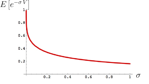
Figure 1. A plot of the expectation value $E\left[e^{-\sigma\,V}\right]$ as given by its explicit expression (21).

Beyond this first result at $\sigma=0$, we can consider, for any $\sigma\geq 0$, the expectation value of $e^{-\sigma\,V}$ for bi-pointed quadrangulations with $N\to\infty$ and finite $s$, conditioned to have their second Voronoï cell finite. It is given by

$$E_{s}\left[e^{-\sigma\,V}\right]=\frac{\sum\limits_{n_{2}}\mathfrak{p}_{s}(n_{2})\,e^{-\sigma\,V}}{\sum\limits_{n_{2}}\mathfrak{p}_{s}(n_{2})}\ ,$$

and has a large $s$ limiting value

$$\begin{split}E_{s}\left[e^{-\sigma\,V}\right]\underset{s\to\infty}{\sim}E\left[e^{-\sigma\,V}\right]&=\frac{[S^{3}]\mathcal{F}\left(S,\sqrt{6},\frac{\sqrt{6}\sigma^{1/4}}{S}\right)}{[S^{3}]\mathcal{F}\left(S,\sqrt{6},0\right)}\\ &=\frac{7}{8}\ [S^{3}]\mathcal{F}\left(S,\sqrt{6},\frac{\sqrt{6}\sigma^{1/4}}{S}\right)\ .\\ \end{split}$$

From the explicit expression of $\mathcal{F}(S,a,b)$ displayed in Appendix A, we deduce after some quite heavy computation the following expression for $E\left[e^{-\sigma\,V}\right]$:

(21) $$\hskip-10.0ptE\left[e^{-\sigma\,V}\right]=\frac{3}{2}\frac{P(\sigma^{1/4})+\sum\limits_{m=1}^{3}\left(P_{m}(\sigma^{1/4},\sqrt{2})\,e^{m\sqrt{6}\,\sigma^{1/4}}+P_{m}(\sigma^{1/4},-\sqrt{2})\,e^{-m\sqrt{6}\,\sigma^{1/4}}\right)}{\left(Q(\sigma^{1/4})\left(4+(4+3\sqrt{2})e^{\sqrt{6}\sigma^{1/4}}+(4-3\sqrt{2})e^{-\sqrt{6}\sigma^{1/4}}\right)-12\right)^{4}}$$

where $P(r)$, $Q(r)$ and $P_{m}(r,\gamma)$ ($m=1,2,3$) are polynomials in $r$ of degree at most $8$ (with coefficients linear in $\gamma$ for the last three polynomials), given explicitly by

$$\begin{split}&\hskip-32.0ptP(r)=96\left(-252-399\sqrt{3}r-756r^{2}-161\sqrt{3}r^{3}+170r^{4}+153\sqrt{3}r^{5}+144r^{6}+22\sqrt{3}r^{7}+4r^{8}\right)\\ \hskip-30.0ptP_{1}(r,\gamma)&=126(168+85\gamma)+63\sqrt{3}\,r\,(867+596\gamma)+1323\,r^{2}\,(132+95\gamma)+28\sqrt{3}\,r^{3}\,(3153+2300\gamma)\\ &+24\,r^{4}\,(2463+1843\gamma)+\sqrt{3}\,r^{5}\,(588+905\gamma)-36\,r^{6}\,(177+124\gamma)-6\sqrt{3}\,r^{7}\,(174+127\gamma)\\ &-36\,r^{8}\,(4+3\gamma)\\ \hskip-30.0ptP_{2}(r,\gamma)&=-8\left(63(24+17\gamma)+63\sqrt{3}\,r\,(105+74\gamma)+378\,r^{2}\,(78+55\gamma)+14\sqrt{3}\,r^{3}\,(1569+1108\gamma)\right.\\ &\left.+12\,r^{4}\,(2337+1652\gamma)+\sqrt{3}\,r^{5}\,(6954+4919\gamma)+18\,r^{6}\,(154+109\gamma)+6\sqrt{3}\,r^{7}\,(24+17\gamma)\right)\\ \hskip-30.0ptP_{3}(r,\gamma)&=126(24+17\gamma)+63\sqrt{3}\,r\,(277+196\gamma)+189\,r^{2}\,(516+365\gamma)+28\sqrt{3}\,r^{3}\,(3399+2404\gamma)\\ &+24\,r^{4}\,(7193+5087\gamma)+\sqrt{3}\,r^{5}\,(68436+48397\gamma)+36\,r^{6}\,(1465+1036\gamma)\\ &+6\sqrt{3}\,r^{7}\,(1342+949\gamma)+12r^{8}(140+99\gamma)\\ &\hskip-30.0ptQ(r)=\left(1+\sqrt{3}r+r^{2}\right)\ .\\ \end{split}$$

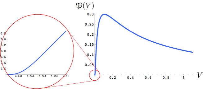
Figure 2. A plot of the probability distribution $\mathfrak{P}(V)$ as obtained from the explicit expression (21) via some numerical inverse Laplace transform. As displayed in the insert, this law becomes flat when $V\to 0$.

The function $E\left[e^{-\sigma\,V}\right]$ is plotted in Figure 1 for illustration. The actual probability distribution $\mathfrak{P}_{s}(V)$ for the rescaled volume $V$ is the inverse Laplace transform of $E_{s}\left[e^{-\sigma\,V}\right]$, hence its large $s$ limit $\mathfrak{P}(V)$ is given by the inverse Laplace transform of $E\left[e^{-\sigma\,V}\right]$. From the quite involved form (21) above, there is no real hope to get an explicit expression for $\mathfrak{P}(V)$ but it may still be plotted thanks to appropriate numerical tools [1, 2, 3]. The resulting shape is displayed in Figure 2. A few analytic properties of $\mathfrak{P}(V)$ may be obtained from its explicit Laplace transform (21) above: in particular, we may easily find large and small $V$ asymptotic equivalents of $\mathfrak{P}(V)$, as discussed now. $\bullet$ The large volume limit. For small $\sigma$, we have the expansion

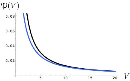
Figure 3. Algebraic decay of $\mathfrak{P}(V)$ at large $V$: the figure displays a comparison between $\mathfrak{P}(V)$ and its large $V$ asymptotic equivalent (in black) given by (22).

$$E\left[e^{-\sigma\,V}\right]=1-\frac{665\sqrt{3}}{1024}\sigma^{1/4}+\frac{49}{768\sqrt{3}}\sigma^{3/4}+\frac{63}{80}\sigma+O(\sigma^{5/4})$$

so that $E\left[e^{-\sigma\,V}\right]$ is not analytic at $\sigma=0$, with all its derivative infinite at this point. We first deduce that all the (positive) moments of $\mathfrak{P}(V)$ are infinite. By a standard argument using the famous Karamata’s tauberian theorem, the large $V$ tail of $\mathfrak{P}(V)$ is estimated from the leading ($\propto\sigma^{1/4}$) small $\sigma$ singularity above as

(22) $$\mathfrak{P}(V)\underset{V\to\infty}{\sim}\frac{665\sqrt{3}}{4096\,\Gamma(3/4)}\,\frac{1}{V^{5/4}}\ .$$

A comparison between $\mathfrak{P}(V)$ (as obtained numerically) and its large $V$ equivalent is displayed in Figure 3. $\bullet$ The mall volume limit. For large $\sigma$, we have the asymptotic equivalence

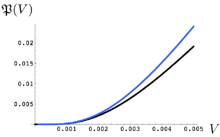
Figure 4. The flat nature of $\mathfrak{P}(V)$ at small $V$: the figure displays a comparison between $\mathfrak{P}(V)$ and its small $V$ equivalent (in black) given by (23).

$$E\left[e^{-\sigma\,V}\right]\underset{\sigma\to\infty}{\sim}\frac{9}{2}(3\sqrt{2}-4)\,e^{-\sqrt{6}\,\sigma^{1/4}}\ .$$

By a simple saddle point calculation (see Appendix C), we deduce the small $V$ estimate

(23) $$\mathfrak{P}(V)\underset{V\to 0}{\sim}\frac{3^{11/6}(3-2\sqrt{2})}{2\sqrt{\pi}}\,\frac{1}{V^{7/6}}\,e^{-\frac{3^{5/3}}{4}\frac{1}{V^{1/3}}}$$

which is a flat function at $V=0$. A comparison between $\mathfrak{P}(V)$ (as obtained numerically) and its small $V$ equivalent is displayed in Figure 4.

4. A comparison with Voronoï cells in infinitely large bi-pointed trees

As an exercise, it is interesting to compare our result for $\mathfrak{P}(V)$ to that, much simpler, obtained for another family of maps, namely bi-pointed plane trees, which are planar maps with a single face and with two marked vertices $v_{1}$ and $v_{2}$, taken again at some fixed even distance $d(v_{1},v_{2})=2s$ along the tree. Any such map is made of a simple path $\mathcal{P}$, formed by the edges joining $v_{1}$ to $v_{2}$, completed by trees attached to the internal vertices of $\mathcal{P}$ on both side of the path and at its extremities $v_{1}$ and $v_{2}$. The two Voronoï cells are now trivially defined by splitting the tree at the “central vertex” in $\mathcal{P}$, which is the vertex along $\mathcal{P}$ lying at distance $s$ from both $v_{1}$ and $v_{2}$ (there are in general two subtrees attached to this vertex and we may decide to split the tree so as to assign one of these subtrees to the first Voronoï cell and the other subtree to the second cell). The volumes $n_{1}$ and $n_{2}$ of the two Voronoï cells are now measured by their number of edges and the generating function $F_{\rm tree}(s,g,h)$ enumerating these maps with a weight $g^{n_{1}}h^{n_{2}}$ reads simply

$$F_{\rm tree}(s,g,h)=\left(g\,\left(R_{\rm tree}\left(g\right)\right)^{2}\right)^{s}\ \left(h\,\left(R_{\rm tree}\left(h\right)\right)^{2}\right)^{s}$$

where $R_{\rm tree}(g)$ is the generating function for planted trees with a weight $g$ per edge, namely

$$R_{\rm tree}(g)=\frac{1-\sqrt{1-4g}}{2g}\ .$$

The scaling function associated with $F_{\rm tree}(s,g,h)$ is obtained by setting

$$g=G_{\rm tree}(a,\epsilon)\ ,\qquad h=G_{\rm tree}(b,\epsilon)\ ,\quad\hbox{where}\ \ G_{\rm tree}(c,\epsilon)\equiv\frac{1}{4}\left(1-\frac{c^{2}}{4}\epsilon^{2}\right)\ ,$$

and reads simply

$$\mathcal{F}_{\rm tree}(S,a,b)=\lim_{\epsilon\to 0}\,F_{\rm tree}\left(\left\lfloor S/\epsilon\right\rfloor,G_{\rm tree}(a,\epsilon),G_{\rm tree}(b,\epsilon)\right)=e^{-(a+b)S}\ .$$

By repeating and adapting the arguments of previous sections, here with leading singularities of type $(1-4g)^{1/2}$, we can find the large $N$ ($=$ total number of edges) asymptotic law $\mathfrak{P}_{\rm tree}(V_{\rm tree})$ for the rescaled volume

$$V_{\rm tree}\equiv\frac{n_{2}}{s^{2}}$$

among bi-pointed trees with $d(v_{1},v_{2})=2s$, conditioned to have their second Voronoï cell finite (which again represent $1/2$ of all bi-pointed trees with fixed $s$). For large $s$, we find (with obvious notations) the expectation value

$$E_{\rm tree}\left[e^{-\sigma\,V_{\rm tree}}\right]=\frac{[S]\mathcal{F}_{\rm tree}\left(S,2,\frac{2\sigma^{1/2}}{S}\right)}{[S]\mathcal{F}_{\rm tree}\left(S,2,0\right)}=e^{-2\sigma^{1/2}}\ .$$

We may now deduce by inverse Laplace transform the exact law for $V_{\rm tree}$

$$\mathfrak{P}_{\rm tree}(V_{\rm tree})=\frac{1}{\sqrt{\pi}\,V_{\rm tree}^{3/2}}e^{-\frac{1}{V_{\rm tree}}}\ ,$$

which is nothing but a simple Lévy distribution. In particular, all its (positive) moments are infinite.

This distribution is a particular member of the more general family of one-sided Lévy distributions with parameter $\alpha$, namely distributions whose Laplace transform is $e^{-{\rm const.}\,p^{\alpha}}$. For $0<\alpha<1$, such distributions are flat at small volume $V$ and vanish as

$$\frac{\hbox{const.}}{V^{(2-\alpha)/(2(1-\alpha))}}\,{\rm exp}\left(-\frac{\hbox{const.'}}{V^{\alpha/(1-\alpha)}}\right)\ .$$

For large volume, they present a fat tail with an algebraic decay of the form $1/V^{1+\alpha}$. The simple law $\mathfrak{P}_{\rm tree}(V)$ for trees corresponds precisely to the situation where $\alpha=1/2$.

As for the distribution $\mathfrak{P}(V)$ of quadrangulations, it is obviously not a Lévy distribution but its small and large $V$ behaviors are nevertheless similar to those obtained for a Lévy distribution with $\alpha=1/4$.

Clearly, the value of $\alpha$ appearing in both the small and large $V$ asymptotics is related to the fractal dimension $D$ of the maps at hand ($D=2$ for trees and $D=4$ for quadrangulations) via

$$\alpha=\frac{1}{D}\ .$$

It is tempting to conjecture that the above forms for small and large $V$ asymptotics should be generic and hold for other families of maps, possibly within more involved universality classes with more general fractal dimensions, hence more general values of $\alpha$.

5. Asymmetric Voronoï cells

In Section 3.3, we estimated the large $N$ asymptotic proportion of bi-pointed planar quadrangulations for which the second Voronoï cell is finite. The obtained value $1/2$ is trivial by symmetry if we assume that configurations for which both Voronoï cells become infinite are negligible (this latter property being de facto proven by the result itself). Note that, in this respect, our computation was performed here in the “worst” situation where the value of the distance $2s$ between the two marked vertices is large.

We may now explicitly break the symmetry and define asymmetric Voronoï cells upon introducing some bias in the measurement of distances. The bijection between bi-pointed planar quadrangulations and planar i-l.2.f.m is indeed only one particular instance of the Miermont bijection. The Miermont bijection allows us to introduce more generally what are called delays, which are integers associated with the marked vertices and allow for some asymmetry in the evaluation of distances [7]. In the case of two marked vertices, two delays may in principle be introduced but, in practice, only their difference (called $\theta$ below) does matter. In the presence of delays, the resulting image of the bi-pointed quadrangulation is again a two-face map, but now with a more general labelling of its vertices by integers. If we insist on keeping a distance $d(v_{1},v_{2})=2s$ between the marked vertices in the original quadrangulation, the labelling of the two-face map, which now involves some additional integer parameter $\theta$, is characterized by the following four properties:

1. labels on adjacent vertices differ by $0$ or $\pm 1$;

2. the minimum label for the set of vertices incident to $f_{1}$ is $1-\theta$;

3. the minimum label for the set of vertices incident to $f_{2}$ is $1+\theta$;

4. the minimum label for the set of vertices incident to $\mathcal{L}$ is $s$;

if $f_{1}$ and $f_{2}$ denote the two faces of the map and $\mathcal{L}$ the loop made of edges incident to both faces. The Miermont bijection is a one-to-one correspondence between bi-pointed planar quadrangulations with $d(v_{1},v_{2})=2s$ and planar two-face maps with a labelling satisfying $(\hbox{L}_{1})-(\hbox{L}_{4})$ above for any fixed $\theta$ in the range [7]

$$-s<\theta<s\ .$$

All the vertices $v$ of the original quadrangulation but $v_{1}$ and $v_{2}$ are recovered in the two-face map, and their label is related to the distance in the quadrangulation via

$$\ell(v)=\min(d(v,v_{1})-\theta,d(v,v_{2})+\theta)\ .$$

Again the two domains of the original quadrangulation covered by $f_{1}$ and $f_{2}$ respectively (upon drawing the quadrangulation and its image via the bijection on top of each other) naturally define two cells in the map. For some generic $\theta$, those are however asymmetric Voronoï cells with the following properties: the first cell now contains all the vertices $v$ such that

$$d(v_{,}v_{1})<d(v,v_{2})+2\theta\quad(\hbox{cell $1$})$$

(this includes the vertex $v_{1}$), as well as a number of vertices satisfying $d(v_{,}v_{1})=d(v,v_{2})+2\theta$. The second cell contains all the vertices $v$ such that

$$d(v_{,}v_{1})>d(v,v_{2})+2\theta\quad(\hbox{cell $2$})$$

(including $v_{2}$) as well as a number of vertices satisfying $d(v_{,}v_{1})=d(v,v_{2})+2\theta$. In particular, the loop $\mathcal{L}$, whose vertices belong to both $f_{1}$ and $f_{2}$, contains only vertices satisfying $d(v_{,}v_{1})=d(v,v_{2})+2\theta$.

Taking $\theta>0$ therefore “favors” cell $1$ whose volume is, on average, larger than that of cell $2$. A control on these volumes is again obtained directly via the bijection by assigning a weight $g$ per edge in $f_{1}$, $h$ per edge in $f_{2}$ and $\sqrt{gh}$ per edge along $\mathcal{L}$. The corresponding generating function reads then

$$\hskip-28.45274ptF(s,\theta,g,h)=\Delta_{u}\Delta_{v}\log(X_{u,v}(g,h))\Big{|}_{u=s+\theta\atop v=s-\theta}=\log\left(\frac{X_{s+\theta,s-\theta}(g,h)X_{s+\theta-1,s-\theta-1}(g,h)}{X_{s+\theta-1,s-\theta}(g,h)X_{s+\theta,s-\theta-1}(g,h)}\right)\ ,$$

giving rise to a scaling function $\mathcal{F}(S,\Theta,a,b)$ via

$$\begin{split}\hskip-28.45274ptF(\left\lfloor S/\epsilon\right\rfloor,\left\lfloor\Theta/\epsilon\right\rfloor,G(a,\epsilon),G(b,\epsilon))&=\epsilon^{3}\,\mathcal{F}(S,\Theta,a,b)+O(\epsilon^{4})\\ \hbox{where}&\quad\mathcal{F}(S,\Theta,a,b)=\frac{1}{3}\ \partial_{U}\partial_{V}x(U,V,a,b)\Big{|}_{U=S+\Theta\atop V=S-\Theta}\ .\\ \end{split}$$

Defining the asymmetry factor $\omega$ by

$$\omega\equiv\frac{\theta}{s}\ ,\quad-1\leq\omega\leq 1\ ,$$

the local limit of configurations with fixed $s$ and $\omega$ is, at large $s$, encoded in the small $S$ expansion of $\mathcal{F}(S,\omega\,S,a,b)$. In particular, we easily get the $b=0$ small $S$ expansion generalizing (20)

$$\begin{split}\mathcal{F}(S,\omega\,S,a,0)&=\frac{1}{2S^{3}}-\frac{a^{4}\,S}{480}(1+\omega)^{3}\left(8-9\omega+3\omega^{2}\right)\\ &+\frac{a^{6}\,S^{3}}{6048}(1+\omega)^{3}\left(32-33\omega+3\omega^{2}+9\omega^{3}-3\omega^{4}\right)+O[S]^{4}\ .\\ \end{split}$$

By the same argument as in Section 3.3, we directly read from the $S^{3}$ coefficient of this expansion the large $s$ probability $\Pi(\omega)$ that, for $N\to\infty$, the volume of the second (now asymmetric with a fixed value of the asymmetry factor $\omega$) Voronoï cell remains finite:

(24) $$\Pi(\omega)=\frac{1}{64}\,(1+\omega)^{3}\left(32-33\omega+3\omega^{2}+9\omega^{3}-3\omega^{4}\right)\ .$$

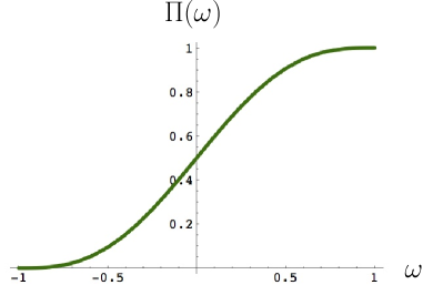
Figure 5. A plot of the probability $\Pi(\omega)$ that the volume of the second Voronoï cell remains finite when $N\to\infty$, as a function of the asymmetry factor $\omega$, as given by (24).

This probability is displayed in Figure 5. It satisfies of course $\Pi(\omega)+\Pi(-\omega)=1$ as expected by symmetry, and in particular $\Pi(0)=1/2$ for the symmetric case. For, say $\omega\to 1$, the second Voronoï cell, which is maximally unfavored by the asymmetry is finite with probability $\Pi(1)=1$.

For a better understanding of the meaning of $\Pi(\omega)$, we may quote Miermont in [7] and “let water flow at unit speed from the sources” $v_{1}$ and $v_{2}$ at given mutual distance $2s$ “in such a way that the water starts diffusing from” $v_{1}$ at time $-\omega\,s$, from $v_{2}$ at time $+\omega\,s$, “and takes unit time to go through an edge. When water currents emanating from different edges meet at a vertex (whenever the water initially comes from the same source of from different sources), they can go on flowing into unvisited edges only (…). The process ends when the water cannot flow any more (…).” In this language, Voronoï cells correspond to domains covered by a given current. When the map volume tends to infinity, only one of the currents flows all the way to infinity, the other current remaining trapped within a finite region. We may then view $\Pi(\omega)$ as the probability for the second current (emanating from the source $v_{2}$) to remain trapped within a finite domain or, equivalently, as the probability for the first current (emanating from the source $v_{1}$) to escape to infinity.

6. conclusion

In this paper, we computed explicitly the value of the expectation value $E\left[e^{-\sigma\,V}\right]$ for infinitely large bi-pointed planar maps, where $V$ is the rescaled volume of that of the two Voronoï cells which remains finite. This law describes Voronoï cells constructed from randomly picked vertices at a prescribed finite mutual distance, and in the limit where this distance is large. Although it may look quite involved, the expression (21) is nevertheless expected to be universal since its derivation entirely relies on properties of scaling functions, which are in fact characteristic of the Brownian map rather than the specific realization at hand (here quadrangulations). In other words, we expect that the same expression (21), up to some possible non-universal normalization for the parameter $\sigma$, would be obtained, in the same regime, for all bi-pointed planar map families in the universality class of so-called pure gravity.

We then deduced from this result a number of features of the associated, universal, volume probability distribution $\mathfrak{P}(V)$, such as its large and small $V$ behaviors (22) and (23). Although we have not been able to give a tractable explicit formula for this law for arbitrary $V$, we thereby showed that its nature is comparable to that of a simple one-sided Lévy distribution with parameter $\alpha=1/4$. Let us conclude by briefly discussing Voronoï cells, now in the so called scaling regime: here we continue to fix the mutual distance $2s$ between the marked vertices but we now let $s$ and $N$ tend simultaneously to infinity with the ratio $S=s/N^{1/4}$ kept finite. In this regime, the fraction $\phi=n_{2}/N$ of the total volume spanned by the second Voronoï cell is again a good measure of the cell volume distribution and the asymptotic law $\mathcal{P}_{\{S\}}(\phi)$ for $\phi$ at fixed $S$ may be obtained as in Section 3.1 via

$$\int_{0}^{1}d\phi\,\mathcal{P}_{\{S\}}(\phi)\,e^{\mu\,\phi}=\lim_{N\to\infty}\frac{[g^{N}]F\left(\left\lfloor SN^{1/4}\right\rfloor,g,g\,e^{\mu/N}\right)}{[g^{N}]F\left(\left\lfloor SN^{1/4}\right\rfloor,g,g\right)}\ .$$

As explained in Appendix B in the context of the local limit law $\mathcal{P}_{s}(\phi)$, the $g^{N}$ coefficient of the numerator above may be extracted via some simple contour integral which, upon taking $g=G(a,1/N^{1/4})$, involves at large $N$ the scaling function $\mathcal{F}(S,a,b)$ at $b=(a^{4}-36\mu)^{1/4}$. This leads to

$$\int_{0}^{1}d\phi\,\mathcal{P}_{\{S\}}(\phi)\,e^{\mu\,\phi}=\frac{\int_{\mathcal{C}_{\mu}}da\,a^{3}\,e^{a^{4}/36}\mathcal{F}(S,a,(a^{4}-36\mu)^{1/4})}{\int_{\mathcal{C}_{0}}da\,a^{3}\,e^{a^{4}/36}\mathcal{F}(S,a,a)}\ ,$$

where the integral over $a$ is over some appropriate contour $\mathcal{C}_{\mu}$ depending on $\mu$ (see Appendix B). Due to the involved expression of $\mathcal{F}(S,a,b)$, we were not able to perform the above contour integrals for general $S$. Still, for $S\to 0$, we recover precisely via a small $S$ expansion the result of Section 3.2 (as expected from the scaling correspondence), now in the form

$$\lim_{S\to 0}\int_{0}^{1}d\phi\,\mathcal{P}_{\{S\}}(\phi)\,e^{\mu\,\phi}=\frac{1}{2}(1+e^{\mu})\quad\Leftrightarrow\quad\lim_{S\to 0}\mathcal{P}_{\{S\}}(\phi)=\frac{1}{2}(\delta(\phi)+\delta(\phi-1))\ .$$

As for the $S\to\infty$ limit, it may be obtained as follows (here we simply give a sketch of the calculation and leave to the reader the task of filling the gaps): from its explicit expression, we have

$$\mathcal{F}(S,a,b)\underset{S\to\infty}{\sim}\mathfrak{Z}(a,b)e^{-(a+b)S}\ ,$$

where the value of the coefficient $\mathfrak{Z}(a,b)$ may easily be obtained but is unimportant for our calculation (apart from the, easily verified property that it has a non-zero limit $\mathfrak{Z}(a,a)$ when $b\to a$). For large $S$, the above contour integrals may be evaluated by a saddle-point method. For the denominator (with $b=a$), we write

$$\frac{d}{da}\left(\frac{a^{4}}{36}-2a\,S\right)\Big{|}_{a=a^{*}}=0\quad\Leftrightarrow\quad(a^{*})^{4}=(18S)^{4/3}$$

and deform the contour $\mathcal{C}_{0}$ so as to pass via the positive real saddle point at $a^{*}=(18S)^{1/3}$. This gives a denominator proportional at large $S$ to $\mathfrak{Z}(a^{*},a^{*})e^{-(18S)^{4/3}/12}$. As for the numerator, it is dominated by the same saddle point but the replacement

$$b\to\left((a^{*})^{4}-36\mu\right)^{1/4}=(18S)^{1/3}-\frac{\mu}{2S}+O\left(\frac{1}{S^{2}}\right)$$

creates a $\mu$-dependent correction. At large $S$, this leads to a numerator now proportional to $\mathfrak{Z}(a^{*},a^{*})e^{-(18S)^{4/3}/12+\mu/2}$ with the same proportionality constant as for the denominator, giving eventually

$$\lim_{S\to\infty}\int_{0}^{1}d\phi\,\mathcal{P}_{\{S\}}(\phi)\,e^{\mu\,\phi}=e^{\mu/2}\quad\Leftrightarrow\quad\lim_{S\to\infty}\mathcal{P}_{\{S\}}(\phi)=\delta(\phi-1/2)\ .$$

This result is quite natural since, heuristically, the limit $S\to\infty$ describes maps with an elongated shape, with the two marked vertices sitting at its extremities. The frontier between the Voronoï cells for such an elongated map is typically a small cycle sitting halfway along the elongated direction, hence splitting the map into two domains of the same volume, equal to half the total volume. It would be interesting to visualize and follow the continuous passage, for increasing $S$, of the distribution $\mathcal{P}_{\{S\}}(\phi)$ from its $S\to 0$ to its $S\to\infty$ limit above and to better understand how its average over arbitrary $S$ (properly weighted by the $S$-dependent two-point function, i.e. the distance profile of the Brownian map) creates the uniform distribution for $\phi\in[0,1]$.

Appendix A Expression for the scaling function $\mathcal{F}(S,a,b)$

The scaling function $x(S,T,a,b)$ was computed in [5] as the appropriate solution of (11). Its explicit expression is quite heavy and is not reproduced here. From this expression, we may obtain $\mathcal{F}(S,a,b)$ directly via (13). It takes the following form:

$$\mathcal{F}(S,a,b)=-\frac{e^{-(a+b)\,S}}{6}\ \frac{\mathfrak{T}(e^{-a\,S},e^{-b\,S},a,b)}{\mathfrak{D}(a,b)}\,\left(\frac{\mathfrak{E}(a,b)}{\mathfrak{U}(e^{-a\,S},e^{-b\,S},a,b)}\right)^{3}\ ,$$

where, introducing the notation

$$c\equiv\sqrt{\frac{a^{2}+b^{2}}{2}}\ ,$$

we have explicitly

$$\begin{split}\hskip-34.14322pt\mathfrak{E}(a,b)&=6\,a\,b\,(a\!-\!b)^{2}(a\!+\!b)\left(2a^{2}\!+\!b^{2}\right)\left(a^{2}\!+\!2b^{2}\right)\ ,\\ \hskip-34.14322pt\mathfrak{D}(a,b)&=(a\!+\!2c)(b\!+\!2c)\left(5a^{3}\!+\!7a^{2}c\!+\!4ab^{2}\!+\!2b^{2}c\right)\left(4a^{2}b\!+\!2a^{2}c\!+\!5b^{3}\!+\!7b^{2}c\right)\\ &\times\left(17a^{2}(a^{2}\!+\!b^{2})\!+\!12a\left(2a^{2}\!+\!b^{2}\right)c\!+\!2b^{4}\right)\left(2a^{4}\!+\!12b\left(a^{2}\!+\!2b^{2}\right)c\!+\!17b^{2}(a^{2}\!+\!b^{2})\right)\ ,\\ \end{split}$$

while $\mathfrak{T}(\sigma,\tau,a,b)$ and $\mathfrak{U}(\sigma,\tau,a,b)$ are polynomials of respective degree $4$ and $2$ in both $\sigma$ and $\tau$, namely

$$\mathfrak{T}(\sigma,\tau,a,b)=\sum_{i=0}^{4}\sum_{j=0}^{4}t_{i,j}\,\sigma^{i}\tau^{j}\quad\hbox{and}\quad\mathfrak{U}(\sigma,\tau,a,b)=\sum_{i=0}^{2}\sum_{j=0}^{2}u_{i,j}\,\sigma^{i}\tau^{j}\ .$$

The coefficients $t_{i,j}\equiv t_{i,j}(a,b)$ and $u_{i,j}\equiv u_{i,j}(a,b)$ may be written for convenience as sums of two contributions:

$$t_{i,j}=t_{i,j}^{(0)}+c\,t_{i,j}^{(1)}\ ,\qquad u_{i,j}=u_{i,j}^{(0)}+c\,u_{i,j}^{(1)}\ ,$$

where we have the explicit expressions

$$\begin{split}&\hskip-34.14322ptt_{0,0}^{(0)}=(a\!+\!b)^{3}(396a^{10}\!+\!1448a^{9}b\!+\!3672a^{8}b^{2}\!+\!6520a^{7}b^{3}\!+\!9135a^{6}b^{4}\!+\!10146a^{5}b^{5}\!+\!9135a^{4}b^{6}\\ &\!+\!6520a^{3}b^{7}\!+\!3672a^{2}b^{8}\!+\!1448ab^{9}\!+\!396b^{10})\\ &\hskip-34.14322ptt_{0,1}^{(0)}=-4(a^{2}\!-\!b^{2})^{2}(198a^{9}\!+\!502a^{8}b\!+\!1099a^{7}b^{2}\!+\!1551a^{6}b^{3}\!+\!1806a^{5}b^{4}\!+\!1596a^{4}b^{5}\\ &\!+\!1128a^{3}b^{6}\!+\!596a^{2}b^{7}\!+\!224ab^{8}\!+\!48b^{9})\\ &\hskip-34.14322ptt_{0,2}^{(0)}=-6b(a^{2}\!-\!b^{2})\left(2a^{2}\!+\!b^{2}\right)(198a^{8}\!+\!280a^{7}b\!+\!611a^{6}b^{2}\!+\!584a^{5}b^{3}\!+\!599a^{4}b^{4}\!+\!368a^{3}b^{5}\\ &\!+\!200a^{2}b^{6}\!+\!64ab^{7}\!+\!12b^{8})\\ &\hskip-34.14322ptt_{0,3}^{(0)}=4a(a^{2}\!-\!b^{2})^{2}\left(2a^{2}\!+\!b^{2}\right)\left(99a^{6}\!+\!29a^{5}b\!+\!186a^{4}b^{2}\!+\!40a^{3}b^{3}\!+\!104a^{2}b^{4}\!+\!12ab^{5}\!+\!16b^{6}\right)\\ &\hskip-34.14322ptt_{0,4}^{(0)}=-(a\!-\!b)^{3}\left(2a^{2}\!+\!b^{2}\right)^{2}\left(99a^{6}-82a^{5}b\!+\!191a^{4}b^{2}-120a^{3}b^{3}\!+\!104a^{2}b^{4}-40ab^{5}\!+\!12b^{6}\right)\\ \end{split}$$

$$\begin{split}&\hskip-34.14322ptt_{1,0}^{(0)}=-4(a^{2}\!-\!b^{2})^{2}(48a^{9}\!+\!224a^{8}b\!+\!596a^{7}b^{2}\!+\!1128a^{6}b^{3}\!+\!1596a^{5}b^{4}\!+\!1806a^{4}b^{5}\\ &\!+\!1551a^{3}b^{6}\!+\!1099a^{2}b^{7}\!+\!502ab^{8}\!+\!198b^{9})\\ &\hskip-34.14322ptt_{1,1}^{(0)}=8(a\!+\!b)^{3}\left(a^{4}\!+\!7a^{2}b^{2}\!+\!b^{4}\right)\left(48a^{6}\!+\!74a^{5}b\!+\!168a^{4}b^{2}\!+\!149a^{3}b^{3}\!+\!168a^{2}b^{4}\!+\!74ab^{5}\!+\!48b^{6}\right)\\ &\hskip-34.14322ptt_{1,2}^{(0)}=-24b(a^{2}\!-\!b^{2})^{2}\left(2a^{2}\!+\!b^{2}\right)\left(24a^{6}\!+\!34a^{5}b\!+\!62a^{4}b^{2}\!+\!54a^{3}b^{3}\!+\!43a^{2}b^{4}\!+\!20ab^{5}\!+\!6b^{6}\right)\\ &\hskip-34.14322ptt_{1,3}^{(0)}=-8a(a\!-\!b)^{2}\left(2a^{2}\!+\!b^{2}\right)\left(a^{4}\!+\!7a^{2}b^{2}\!+\!b^{4}\right)\left(24a^{4}\!+\!7a^{3}b\!+\!33a^{2}b^{2}\!+\!6ab^{3}\!+\!10b^{4}\right)\\ &\hskip-34.14322ptt_{1,4}^{(0)}=4(a^{2}\!-\!b^{2})^{2}\left(2a^{2}\!+\!b^{2}\right)^{2}\left(12a^{5}-22a^{4}b\!+\!27a^{3}b^{2}-27a^{2}b^{3}\!+\!14ab^{4}-6b^{5}\right)\\ \end{split}$$

$$\begin{split}&\hskip-34.14322ptt_{2,0}^{(0)}=6a(a^{2}\!-\!b^{2})\left(a^{2}\!+\!2b^{2}\right)(12a^{8}\!+\!64a^{7}b\!+\!200a^{6}b^{2}\!+\!368a^{5}b^{3}\!+\!599a^{4}b^{4}\!+\!584a^{3}b^{5}\\ &\!+\!611a^{2}b^{6}\!+\!280ab^{7}\!+\!198b^{8})\\ &\hskip-34.14322ptt_{2,1}^{(0)}=-24a(a^{2}\!-\!b^{2})^{2}\left(a^{2}\!+\!2b^{2}\right)\left(6a^{6}\!+\!20a^{5}b\!+\!43a^{4}b^{2}\!+\!54a^{3}b^{3}\!+\!62a^{2}b^{4}\!+\!34ab^{5}\!+\!24b^{6}\right)\\ &\hskip-34.14322ptt_{2,2}^{(0)}=0\\ &\hskip-34.14322ptt_{2,3}^{(0)}=24a^{2}(a^{2}\!-\!b^{2})^{2}\left(2a^{2}\!+\!b^{2}\right)\left(a^{2}\!+\!2b^{2}\right)\left(3a^{3}-2a^{2}b\!+\!2ab^{2}-2b^{3}\right)\\ &\hskip-34.14322ptt_{2,4}^{(0)}=-6a(a^{2}\!-\!b^{2})\left(2a^{2}\!+\!b^{2}\right)^{2}\left(a^{2}\!+\!2b^{2}\right)\left(3a^{4}-8a^{3}b\!+\!11a^{2}b^{2}-8ab^{3}\!+\!6b^{4}\right)\\ \end{split}$$

$$\begin{split}&\hskip-34.14322ptt_{3,0}^{(0)}=4b(a^{2}\!-\!b^{2})^{2}\left(a^{2}\!+\!2b^{2}\right)\left(16a^{6}\!+\!12a^{5}b\!+\!104a^{4}b^{2}\!+\!40a^{3}b^{3}\!+\!186a^{2}b^{4}\!+\!29ab^{5}\!+\!99b^{6}\right)\\ &\hskip-34.14322ptt_{3,1}^{(0)}=-8b(a\!-\!b)^{2}\left(a^{2}\!+\!2b^{2}\right)\left(a^{4}\!+\!7a^{2}b^{2}\!+\!b^{4}\right)\left(10a^{4}\!+\!6a^{3}b\!+\!33a^{2}b^{2}\!+\!7ab^{3}\!+\!24b^{4}\right)\\ &\hskip-34.14322ptt_{3,2}^{(0)}=-24b^{2}(a^{2}\!-\!b^{2})^{2}\left(2a^{2}\!+\!b^{2}\right)\left(a^{2}\!+\!2b^{2}\right)\left(2a^{3}\!-\!2a^{2}b\!+\!2ab^{2}\!-\!3b^{3}\right)\\ &\hskip-34.14322ptt_{3,3}^{(0)}=-8ab(a\!+\!b)^{3}\left(2a^{2}\!+\!b^{2}\right)\left(a^{2}\!+\!2b^{2}\right)\left(a^{4}\!+\!7a^{2}b^{2}\!+\!b^{4}\right)\\ &\hskip-34.14322ptt_{3,4}^{(0)}=4b(a^{2}\!-\!b^{2})^{2}\left(2a^{2}\!+\!b^{2}\right)^{2}\left(a^{2}\!+\!2b^{2}\right)\left(2a^{2}-ab\!+\!3b^{2}\right)\\ \end{split}$$

$$\begin{split}&\hskip-34.14322ptt_{4,0}^{(0)}=(a\!-\!b)^{3}\left(a^{2}\!+\!2b^{2}\right)^{2}\left(12a^{6}-40a^{5}b\!+\!104a^{4}b^{2}-120a^{3}b^{3}\!+\!191a^{2}b^{4}-82ab^{5}\!+\!99b^{6}\right)\\ &\hskip-34.14322ptt_{4,1}^{(0)}=-4(a^{2}-b^{2})^{2}\left(a^{2}+2b^{2}\right)^{2}\left(6a^{5}-14a^{4}b+27a^{3}b^{2}-27a^{2}b^{3}+22ab^{4}-12b^{5}\right)\\ &\hskip-34.14322ptt_{4,2}^{(0)}=6b(a^{2}\!-\!b^{2})\left(2a^{2}\!+\!b^{2}\right)\left(a^{2}\!+\!2b^{2}\right)^{2}\left(6a^{4}-8a^{3}b\!+\!11a^{2}b^{2}-8ab^{3}\!+\!3b^{4}\right)\\ &\hskip-34.14322ptt_{4,3}^{(0)}=4a(a^{2}-b^{2})^{2}\left(2a^{2}+b^{2}\right)\left(a^{2}+2b^{2}\right)^{2}\left(3a^{2}-ab+2b^{2}\right)\\ &\hskip-34.14322ptt_{4,4}^{(0)}=-(a\!+\!b)^{3}\left(2a^{2}\!+\!b^{2}\right)^{2}\left(a^{2}\!+\!2b^{2}\right)^{2}\left(3a^{2}\!+\!2ab\!+\!3b^{2}\right)\\ \end{split}$$

and

$$\begin{split}&\hskip-34.14322ptt_{0,0}^{(1)}=4(a\!+\!b)^{4}\left(10a^{4}\!+\!18a^{3}b\!+\!25a^{2}b^{2}\!+\!18ab^{3}\!+\!10b^{4}\right)\left(14a^{4}\!+\!12a^{3}b\!+\!29a^{2}b^{2}\!+\!12ab^{3}\!+\!14b^{4}\right)\\ &\hskip-34.14322ptt_{0,1}^{(1)}=-4(a^{2}\!-\!b^{2})^{2}(280a^{8}\!+\!710a^{7}b\!+\!1414a^{6}b^{2}\!+\!1839a^{5}b^{3}\!+\!1881a^{4}b^{4}\!+\!1428a^{3}b^{5}\!+\!812a^{2}b^{6}\\ &\!+\!316ab^{7}\!+\!68b^{8})\\ &\hskip-34.14322ptt_{0,2}^{(1)}=-24b(a^{2}\!-\!b^{2})\left(2a^{2}\!+\!b^{2}\right)\left(10a^{3}\!+\!7a^{2}b\!+\!8ab^{2}\!+\!2b^{3}\right)\left(7a^{4}\!+\!5a^{3}b\!+\!9a^{2}b^{2}\!+\!4ab^{3}\!+\!2b^{4}\right)\\ &\hskip-34.14322ptt_{0,3}^{(1)}=4(a^{2}\!-\!b^{2})^{2}\left(2a^{2}\!+\!b^{2}\right)\left(140a^{6}\!+\!41a^{5}b\!+\!193a^{4}b^{2}\!+\!36a^{3}b^{3}\!+\!68a^{2}b^{4}\!+\!4ab^{5}\!+\!4b^{6}\right)\\ &\hskip-34.14322ptt_{0,4}^{(1)}=-4(a\!-\!b)^{3}\left(2a^{2}\!+\!b^{2}\right)^{2}\left(5a^{2}-2ab\!+\!2b^{2}\right)\left(7a^{3}-3a^{2}b\!+\!6ab^{2}-2b^{3}\right)\\ \end{split}$$

$$\begin{split}&\hskip-34.14322ptt_{1,0}^{(1)}=-4(a^{2}\!-\!b^{2})^{2}(68a^{8}\!+\!316a^{7}b\!+\!812a^{6}b^{2}\!+\!1428a^{5}b^{3}\!+\!1881a^{4}b^{4}\!+\!1839a^{3}b^{5}\!+\!1414a^{2}b^{6}\\ &\!+\!710ab^{7}\!+\!280b^{8})\\ &\hskip-34.14322ptt_{1,1}^{(1)}=16(a\!+\!b)^{2}\left(a^{4}\!+\!7a^{2}b^{2}\!+\!b^{4}\right)\left(34a^{6}\!+\!86a^{5}b\!+\!155a^{4}b^{2}\!+\!179a^{3}b^{3}\!+\!155a^{2}b^{4}\!+\!86ab^{5}\!+\!34b^{6}\right)\\ &\hskip-34.14322ptt_{1,2}^{(1)}=-24b(a^{2}\!-\!b^{2})^{2}\left(2a^{2}\!+\!b^{2}\right)\left(34a^{5}\!+\!48a^{4}b\!+\!71a^{3}b^{2}\!+\!52a^{2}b^{3}\!+\!30ab^{4}\!+\!8b^{5}\right)\\ &\hskip-34.14322ptt_{1,3}^{(1)}=-16(a\!-\!b)^{2}\left(2a^{2}\!+\!b^{2}\right)\left(a^{4}\!+\!7a^{2}b^{2}\!+\!b^{4}\right)\left(17a^{4}\!+\!5a^{3}b\!+\!15a^{2}b^{2}\!+\!2ab^{3}\!+\!2b^{4}\right)\\ &\hskip-34.14322ptt_{1,4}^{(1)}=4(a^{2}\!-\!b^{2})^{2}\left(2a^{2}\!+\!b^{2}\right)^{2}\left(17a^{4}-31a^{3}b\!+\!30a^{2}b^{2}-22ab^{3}\!+\!8b^{4}\right)\\ \end{split}$$

$$\begin{split}&\hskip-34.14322ptt_{2,0}^{(1)}=24a(a^{2}\!-\!b^{2})\left(a^{2}\!+\!2b^{2}\right)\left(2a^{3}\!+\!8a^{2}b\!+\!7ab^{2}\!+\!10b^{3}\right)\left(2a^{4}\!+\!4a^{3}b\!+\!9a^{2}b^{2}\!+\!5ab^{3}\!+\!7b^{4}\right)\\ &\hskip-34.14322ptt_{2,1}^{(1)}=-24a(a^{2}\!-\!b^{2})^{2}\left(a^{2}\!+\!2b^{2}\right)\left(8a^{5}\!+\!30a^{4}b\!+\!52a^{3}b^{2}\!+\!71a^{2}b^{3}\!+\!48ab^{4}\!+\!34b^{5}\right)\\ &\hskip-34.14322ptt_{2,2}^{(1)}=0\\ &\hskip-34.14322ptt_{2,3}^{(1)}=24a(a^{2}\!-\!b^{2})^{2}\left(2a^{2}\!+\!b^{2}\right)\left(a^{2}\!+\!2b^{2}\right)\left(4a^{3}-3a^{2}b-2b^{3}\right)\\ &\hskip-34.14322ptt_{2,4}^{(1)}=-24a(a-2b)(a^{2}\!-\!b^{2})\left(2a^{2}\!+\!b^{2}\right)^{2}\left(a^{2}\!+\!2b^{2}\right)\left(a^{2}-ab\!+\!b^{2}\right)\\ \end{split}$$

$$\begin{split}&\hskip-34.14322ptt_{3,0}^{(1)}=4(a^{2}\!-\!b^{2})^{2}\left(a^{2}\!+\!2b^{2}\right)\left(4a^{6}\!+\!4a^{5}b\!+\!68a^{4}b^{2}\!+\!36a^{3}b^{3}\!+\!193a^{2}b^{4}\!+\!41ab^{5}\!+\!140b^{6}\right)\\ &\hskip-34.14322ptt_{3,1}^{(1)}=-16(a\!-\!b)^{2}\left(a^{2}\!+\!2b^{2}\right)\left(a^{4}\!+\!7a^{2}b^{2}\!+\!b^{4}\right)\left(2a^{4}\!+\!2a^{3}b\!+\!15a^{2}b^{2}\!+\!5ab^{3}\!+\!17b^{4}\right)\\ &\hskip-34.14322ptt_{3,2}^{(1)}=-24b(a^{2}\!-\!b^{2})^{2}\left(2a^{2}\!+\!b^{2}\right)\left(a^{2}\!+\!2b^{2}\right)\left(2a^{3}\!+\!3ab^{2}-4b^{3}\right)\\ &\hskip-34.14322ptt_{3,3}^{(1)}=16(a\!+\!b)^{2}\left(2a^{2}\!+\!b^{2}\right)\left(a^{2}\!+\!2b^{2}\right)\left(a^{2}-ab\!+\!b^{2}\right)\left(a^{4}\!+\!7a^{2}b^{2}\!+\!b^{4}\right)\\ &\hskip-34.14322ptt_{3,4}^{(1)}=-4(a^{2}\!-\!b^{2})^{2}\left(2a^{2}\!+\!b^{2}\right)^{2}\left(a^{2}\!+\!2b^{2}\right)\left(a^{2}-ab\!+\!4b^{2}\right)\\ \end{split}$$

$$\begin{split}&\hskip-34.14322ptt_{4,0}^{(1)}=-4(a\!-\!b)^{3}\left(a^{2}\!+\!2b^{2}\right)^{2}\left(2a^{2}-2ab\!+\!5b^{2}\right)\left(2a^{3}-6a^{2}b\!+\!3ab^{2}-7b^{3}\right)\\ &\hskip-34.14322ptt_{4,1}^{(1)}=4(a^{2}\!-\!b^{2})^{2}\left(a^{2}\!+\!2b^{2}\right)^{2}\left(8a^{4}\!-\!22a^{3}b\!+\!30a^{2}b^{2}\!-\!31ab^{3}\!+\!17b^{4}\right)\\ &\hskip-34.14322ptt_{4,2}^{(1)}=-24b(2a\!-\!b)(a^{2}\!-\!b^{2})\left(2a^{2}\!+\!b^{2}\right)\left(a^{2}\!+\!2b^{2}\right)^{2}\left(a^{2}-ab\!+\!b^{2}\right)\\ &\hskip-34.14322ptt_{4,3}^{(1)}=-4(a^{2}\!-\!b^{2})^{2}\left(2a^{2}\!+\!b^{2}\right)\left(a^{2}\!+\!2b^{2}\right)^{2}\left(4a^{2}\!-\!ab\!+\!b^{2}\right)\\ &\hskip-34.14322ptt_{4,4}^{(1)}=4(a\!+\!b)^{4}\left(2a^{2}\!+\!b^{2}\right)^{2}\left(a^{2}\!+\!2b^{2}\right)^{2}\ ,\\ \end{split}$$

together with

$$\begin{split}&\hskip-34.14322ptu_{0,0}^{(0)}=-(a\!-\!b)^{2}(a\!+\!b)\left(2a^{2}\!+\!b^{2}\right)\left(a^{2}\!+\!2b^{2}\right)\\ &\hskip-34.14322ptu_{0,1}^{(0)}=4(a\!-\!b)^{2}(a\!+\!b)\left(a^{2}\!+\!2b^{2}\right)^{2}\\ &\hskip-34.14322ptu_{0,2}^{(0)}=-(a\!-\!b)\left(a^{2}\!+\!2b^{2}\right)\left(2a^{4}\!+\!17a^{2}b^{2}\!+\!17b^{4}\right)\\ &\hskip-34.14322ptu_{1,0}^{(0)}=4(a\!-\!b)^{2}(a\!+\!b)\left(2a^{2}\!+\!b^{2}\right)^{2}\\ &\hskip-34.14322ptu_{1,1}^{(0)}=-8(a\!+\!b)\left(4a^{2}\!+\!ab\!+\!4b^{2}\right)\left(a^{4}\!+\!7a^{2}b^{2}\!+\!b^{4}\right)\\ &\hskip-34.14322ptu_{1,2}^{(0)}=4(a^{2}\!-\!b^{2})\left(4a^{5}\!+\!14a^{4}b\!+\!22a^{3}b^{2}\!+\!32a^{2}b^{3}\!+\!19ab^{4}\!+\!17b^{5}\right)\\ &\hskip-34.14322ptu_{2,0}^{(0)}=(a\!-\!b)\left(2a^{2}\!+\!b^{2}\right)\left(17a^{4}\!+\!17a^{2}b^{2}\!+\!2b^{4}\right)\\ &\hskip-34.14322ptu_{2,1}^{(0)}=-4(a^{2}\!-\!b^{2})\left(17a^{5}\!+\!19a^{4}b\!+\!32a^{3}b^{2}\!+\!22a^{2}b^{3}\!+\!14ab^{4}\!+\!4b^{5}\right)\\ &\hskip-34.14322ptu_{2,2}^{(0)}=(a\!+\!b)\left(34a^{6}\!+\!76a^{5}b\!+\!137a^{4}b^{2}\!+\!154a^{3}b^{3}\!+\!137a^{2}b^{4}\!+\!76ab^{5}\!+\!34b^{6}\right)\\ \end{split}$$

and

$$\begin{split}&\hskip-34.14322ptu_{0,0}^{(1)}=0\\ &\hskip-34.14322ptu_{0,1}^{(1)}=-12b(a\!-\!b)^{2}(a\!+\!b)\left(a^{2}\!+\!2b^{2}\right)\\ &\hskip-34.14322ptu_{0,2}^{(1)}=12b(a\!-\!b)\left(a^{2}\!+\!2b^{2}\right)^{2}\\ &\hskip-34.14322ptu_{1,0}^{(1)}=-12a(a\!-\!b)^{2}(a\!+\!b)\left(2a^{2}\!+\!b^{2}\right)\\ &\hskip-34.14322ptu_{1,1}^{(1)}=48\left(a^{2}\!+\!ab\!+\!b^{2}\right)\left(a^{4}\!+\!7a^{2}b^{2}\!+\!b^{4}\right)\\ &\hskip-34.14322ptu_{1,2}^{(1)}=-12(a^{2}\!-\!b^{2})\left(2a^{4}\!+\!6a^{3}b\!+\!11a^{2}b^{2}\!+\!9ab^{3}\!+\!8b^{4}\right)\\ &\hskip-34.14322ptu_{2,0}^{(1)}=-12a(a\!-\!b)\left(2a^{2}\!+\!b^{2}\right)^{2}\\ &\hskip-34.14322ptu_{2,1}^{(1)}=12(a^{2}\!-\!b^{2})\left(8a^{4}\!+\!9a^{3}b\!+\!11a^{2}b^{2}\!+\!6ab^{3}\!+\!2b^{4}\right)\\ &\hskip-34.14322ptu_{2,2}^{(1)}=-12(a\!+\!b)^{2}\left(a^{2}\!+\!ab\!+\!b^{2}\right)\left(4a^{2}\!+\!ab\!+\!4b^{2}\right)\ .\\ \end{split}$$

Appendix B Calculation of the law for $\phi=n_{2}/N$ in the local limit

Our starting point is the expansion of $X_{s,t}(G(a,\epsilon),G(b,\epsilon))$ when $\epsilon\to 0$, with $G(c,\epsilon)$ as in (5). Expanding the equation (2) to increasing orders in $\epsilon$, we deduce the expansion

$$X_{s,t}(G(a,\epsilon),G(b,\epsilon))=\frac{3(s+1)(t+1)(s+t+3)}{(s+3)(t+3)(s+t+1)}+\sum_{i\geq 1}\mathfrak{X}_{i}(s,t,a,b)\epsilon^{2i}\ ,$$

where the first term is easily deduced from $\epsilon$ the exact expression (4) with $g=h=1/12$ and where the $\mathfrak{X}_{i}$’s are obtained recursively, order by order in $\epsilon^{2}$.

Expanding (2) at order $\epsilon^{2}$ shows that $\mathfrak{X}_{1}(s,t,a,b)=0$ and, at order $\epsilon^{4}$, that $\mathfrak{X}_{2}$ may be written (by linearity) as

$$\mathfrak{X}_{2}(s,t,a,b)=a^{4}\xi(s,t)+b^{4}\xi(t,s)\ ,$$

where $\xi(s,t)$ is the solution of some appropriate partial differential equation. We thus have the following form for the first terms in the expansion:

$$\begin{split}X_{s,t}(G(a,\epsilon),G(b,\epsilon))=\frac{3(s+1)(t+1)(s+t+3)}{(s+3)(t+3)(s+t+1)}&+(a^{4}\xi(s,t)+b^{4}\xi(t,s))\epsilon^{4}\\ &+\mathfrak{X}_{3}(s,t,a,b)\epsilon^{6}+O(\epsilon^{8})\ ,\\ \end{split}$$

from which we deduce via (1) the expansion

$$F(s,G(a,\epsilon),G(b,\epsilon))=\log\left(\frac{s^{2}(2s+3)}{(s+1)^{2}(2s-1)}\right)-(a^{4}+b^{4})\psi(s)\,\epsilon^{4}+\mathfrak{F}_{3}(s,a,b)\epsilon^{6}+O(\epsilon^{8})\ ,$$

where $\psi(s)$ is directly related to $\xi(s,t)$ and $\mathfrak{F}_{3}(s,a,b)$ to $\mathfrak{X}_{3}(s,t,a,b)$. From the very existence of the scaling function, we may write

(25) $$\begin{split}\mathcal{F}(S,a,b)&=\lim_{\epsilon\to 0}\,\frac{1}{\epsilon^{3}}\,F\left(\left\lfloor S/\epsilon\right\rfloor,G(a,\epsilon),G(b,\epsilon)\right)\\ &=\frac{1}{2\,S^{3}}+(a^{4}+b^{4})\,\lim_{\epsilon\to 0}\epsilon\,\psi\left(\left\lfloor S/\epsilon\right\rfloor\right)+\lim_{\epsilon\to 0}\left(\epsilon^{3}\mathfrak{F}_{3}\left(\left\lfloor S/\epsilon\right\rfloor,a,b\right)+O(\epsilon^{5})\right)\ .\\ \end{split}$$

This is to be compared with the small $S$ expansion of $\mathcal{F}(S,a,b)$, as obtained from its exact expression of Appendix A, namely

$$\mathcal{F}(S,a,b)=\frac{1}{2\,S^{3}}-(a^{4}+b^{4})\,\frac{S}{60}+(a^{6}+b^{6})\,\frac{S^{3}}{189}+O(S^{5})\ .$$

We readily deduce that $\psi(s)\sim s/60$ when $s\to\infty$ and

$$\mathfrak{F}_{3}(s,a,b)\underset{s\to\infty}{\sim}(a^{6}+b^{6})\,\frac{s^{3}}{189}$$

(note that the $O(\epsilon^{5})$ term in (25) necessarily leads to an $O(S^{5})$ term in $\mathcal{F}(S,a,b)$), which is precisely the announced scaling correspondence.

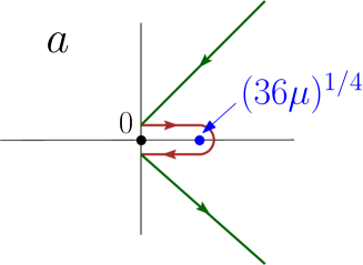
Figure 6. Contour of integration in the complex plane for the variable $a$, as inherited from the contour in $g$ around $0$ in the contour integral (26) via the change of variable $g=G(a,\epsilon)$ when $\epsilon=1/N\to 0$ (see [5]).

We may now estimate $[g^{N}]F(s,g,g\,e^{\mu/N})$.This quantity is obtained by a contour integral around $g=0$, namely

(26) $$\frac{1}{2\rm{i}\pi}\oint\frac{dg}{g^{N+1}}F(s,g,g\,e^{\frac{\mu}{N}})$$

and, at large $N$, we may change variable from $g$ to $a$ by taking $g=G(a,\epsilon)$ with

$$\hskip 142.26378pt\epsilon=\frac{1}{N^{1/4}}\ .$$

Setting $h=g\,e^{\frac{\mu}{N}}=g\,(1+\mu\epsilon^{4})$ then amounts to choosing

$$\frac{-b^{4}}{36}=\frac{-a^{4}}{36}+\mu+O\left(\frac{1}{N}\right)\quad\Leftrightarrow\quad b^{4}=a^{4}-36\mu+O\left(\frac{1}{N}\right)\ .$$

Using $dg=-(1/12)a^{3}/(9N)$ and $g^{N+1}\sim(1/12)^{N+1}\,e^{-a^{4}/36}$, we eventually arrive at

$$\begin{split}[g^{N}]F(s,g,g\,e^{\mu/N})&=\frac{1}{2\rm{i}\pi}\frac{12^{N}}{N}\int_{\mathcal{C}_{\mu}}da\,\frac{-a^{3}}{9}\,e^{a^{4}/36}\Big{\{}\log\left(\frac{s^{2}(2s+3)}{(s+1)^{2}(2s-1)}\right)\\ &-\frac{1}{N}\,(2a^{4}-36\mu)\psi(s)+\frac{1}{N^{3/2}}\mathfrak{F}_{3}(s,a,(a^{4}-36\mu)^{1/4})+O\left(\frac{1}{N^{2}}\right)\Big{\}}\\ \end{split}$$

with some appropriate integration contour $\mathcal{C}_{\mu}$ in the complex plane. As explained in [5] and illustrated in Figure 6, this contour is made of a first part $\mathcal{C}_{\mu,1}$ consisting of two half straight lines at $\pm 45^{\circ}$ meeting at the origin, and a part $\mathcal{C}_{\mu,2}$ which makes a back and forth excursion from $0$ to $(36\mu)^{1/4}$. Both the constant (i.e. independent of $a$) terms and the $a^{4}$ term in-between the curly brackets lead to integrals along this contour which vanish identically by symmetry, so that

$$[g^{N}]F(s,g,g\,e^{\mu/N})\underset{N\to\infty}{\sim}\frac{1}{2\rm{i}\pi}\frac{12^{N}}{N^{5/2}}\int_{\mathcal{C}_{\mu}}da\,\frac{-a^{3}}{9}\,e^{a^{4}/36}\mathfrak{F}_{3}(s,a,(a^{4}-36\mu)^{1/4})$$

with a right hand side which behaves at large $s$ as

$$\hskip-34.14322pt\frac{1}{2\rm{i}\pi}\int_{\mathcal{C}_{\mu}}da\,\frac{-a^{3}}{9}\,e^{a^{4}/36}\mathfrak{F}_{3}(s,a,(b^{4}\!-\!36\mu)^{1/4})\underset{s\to\infty}{\sim}\frac{s^{3}}{189}\frac{1}{2\rm{i}\pi}\int_{\mathcal{C}_{\mu}}da\,\frac{-a^{3}}{9}\,e^{a^{4}/36}(a^{6}+(a^{4}\!-\!36\mu)^{3/2})\ .$$

The contribution of the two terms in this latter integral were computed in [5], namely

$$\begin{split}&\frac{1}{2\rm{i}\pi}\int_{\mathcal{C}_{\mu}}da\,\frac{-a^{3}}{9}\,e^{a^{4}/36}a^{6}=\frac{432}{\pi}\,\int_{0}^{\infty}dt\,t^{4}e^{-t^{2}}=\frac{162}{\sqrt{\pi}}\ ,\\ &\frac{1}{2\rm{i}\pi}\int_{\mathcal{C}_{\mu}}da\,\frac{-a^{3}}{9}\,e^{a^{4}/36}(a^{4}\!-\!36\mu)^{3/2}=\frac{432\,e^{\mu}}{\pi}\,\int_{0}^{\infty}dt\,t^{4}e^{-t^{2}}=\frac{162}{\sqrt{\pi}}\,e^{\mu}\ .\\ \end{split}$$

This yields eventually

$$[g^{N}]F(s,g,g\,e^{\mu/N})\underset{N\to\infty}{\sim}\frac{12^{N}}{\sqrt{\pi}\,N^{5/2}}\left(\frac{6}{7}(1+e^{\mu})\,s^{3}+O(s^{2})\right)$$

at large $s$. At $\mu=0$, we recover the estimate (8). Taking the appropriate ratio, we arrive immediately at the desired result (14).

Appendix C Estimate of $\mathfrak{P}(V)$ at small $V$

Since the quantity

$$\hat{\mathfrak{P}}(\sigma)\equiv E\left[e^{-\sigma\,V}\right]$$

is the Laplace transform of the probability distribution $\mathfrak{P}(V)$, with $V$ taking its values in $[0,\infty)$, it has no singularity for real non-negative $\sigma$. Its inverse Laplace transform, the probability distribution $\mathfrak{P}(V)$ itself, may thus be obtained via

$$\mathfrak{P}(V)=\frac{1}{2\rm{i}\pi}\int_{\gamma-\rm{i}\infty}^{\gamma+\rm{i}\infty}d\sigma\,e^{\sigma\,V}\,\hat{\mathfrak{P}}(\sigma)$$

for any real non-negative $\gamma$. At small $V$, this integral may be evaluated via a saddle point approximation as follows. For large $\sigma$, we have the asymptotic equivalence

$$\hat{\mathfrak{P}}(\sigma)\underset{\sigma\to\infty}{\sim}\frac{9}{2}(3\sqrt{2}-4)\,e^{-\sqrt{6}\,\sigma^{1/4}}$$

and the integral is dominated by its saddle point $\sigma^{*}$ given by

$$\frac{d\ }{d\sigma}\left(\sigma\,V-\sqrt{6}\,\sigma^{1/4}\right)\Big{|}_{\sigma=\sigma^{*}}=0\quad\Leftrightarrow\quad\sigma^{*}=\frac{3^{2/3}}{4V^{4/3}}\ .$$

The use of the asymptotic equivalent above for $\hat{\mathfrak{P}}(\sigma)$ is fully consistent if $\sigma^{*}$ becomes large, i.e. when $V$ itself becomes small. Setting

$$\sigma=\sigma^{*}+\rm{i}\,\eta$$

in the integral, with $\eta$ real (i.e. choosing implicitly $\gamma=\sigma^{*}$), we may use the expansion

$$\sigma\,V-\sqrt{6}\,\sigma^{1/4}=-\frac{3^{5/3}}{4\,V^{1/3}}-\frac{3^{1/3}}{2}\,V^{7/3}\,\eta^{2}+O\left(\eta^{3}\right)$$

to write

$$\begin{split}\mathfrak{P}(V)\underset{V\to 0}{\sim}&\ \frac{9}{2}(3\sqrt{2}-4)\,e^{-\frac{3^{5/3}}{4\,V^{1/3}}}\frac{1}{2\pi}\int_{-\infty}^{\infty}d\eta\,e^{-\frac{3^{1/3}}{2}\,V^{7/3}\,\eta^{2}}\\ &=\frac{3^{11/6}(3-2\sqrt{2})}{2\sqrt{\pi}}\,\frac{1}{V^{7/6}}\,e^{-\frac{3^{5/3}}{4}\frac{1}{V^{1/3}}}\ .\\ \end{split}$$

References

- [1] J. Abate and P. P. Valkó. Mathematica packages “Numerical Laplace Inversion” and “Numerical Inversion of Laplace Transform with Multiple Precision Using the Complex Domain”, available on the Wolfram Library Archive: http://library.wolfram.com/infocenter/MathSource/4738/ and http://library.wolfram.com/infocenter/MathSource/5026/ .
- [2] J. Abate and P. P. Valkó. Comparison of sequence accelerators for the Gaver method of numerical Laplace transform inversion. Computers & Mathematics with Applications, 48(3):629 – 636, 2004.
- [3] J. Abate and P. P. Valkó. Multi-precision Laplace transform inversion. International Journal for Numerical Methods in Engineering, 60(5):979–993, 2004.
- [4] G. Chapuy. On tessellations of random maps and the -recurrence, 2016. arXiv:1603.07714 [math.PR].
- [5] E. Guitter. On a conjecture by Chapuy about voronoi cells in large maps, 2017. arXiv:1703.02781 [math.CO].
- [6] E. Guitter. Refined universal laws for hull volumes and perimeters in large planar maps. Journal of Physics A: Mathematical and Theoretical, 50(27):275203, 2017.
- [7] G. Miermont. Tessellations of random maps of arbitrary genus. Ann. Sci. Éc. Norm. Supér. (4), 42(5):725–781, 2009.