Local contractivity of the $\Phi_{4}^{4}$ mapping

Abstract

We show the existence and uniqueness of a solution to a $\Phi_{4}^{4}$ non linear renormalized system of equations of motion in Euclidean space. This system represents a non trivial model which describes the dynamics of the $\Phi_{4}^{4}$ Green’s functions in the Axiomatic Quantum Field Theory (AQFT) framework.

The main argument is the local contractivity of the so called “new mapping” in the neighborhood of a particular “tree type” sequence of Green’s functions. This neighborhood (and the $\Phi_{4}^{4}$ non trivial solution) belongs to a particular subset of the appropriate Banach space characterized by signs, splitting (analogous to that of the $\Phi_{0}^{4}$ solution), axiomatic analyticity properties and “good” asymptotic behavior with respect to the four-dimensional euclidean external momenta.

1 Introduction

1 A new non perturbative method

Several years ago we initiated a program for the construction of a nontrivial $\Phi^{4}_{4}$ model consistent with the general principles of a Wightman Quantum Field Theory ($Q.F.T.$) [1]. In references [2] we introduced a non perturbative method for the construction of a nontrivial solution of the system of the $\Phi^{4}$ equations of motion for the Green’s functions, in the Euclidean space of zero, one and two dimensions. In references [3] we tried to apply an extension of this method to the case of a four (and a fortiori of a three)-dimensional Euclidean momentum space through the proof of a global contractivity principle inside an appropriate Banach space. However that method was rather complicated and also could profit from more precise norm definitions.

Using a Banach space “analogous” to that of zero dimensions and the local contractivity of the mapping (renormalized equations of motion in four -dimensional problem) in a neighbourhoud of the zero dimensional solution, we will be able to present an easily convincing proof of the $\Phi^{4}_{4}$ nontriviality.

This method is different in approach from the work done in the Constructive $Q.F.T.$ framework of Glimm-Jaffe and others [4] [5], and the methods of Symanzik who created the basis for a pure Euclidean approach to $Q.F.T.$ [6].

In the $Q.F.T.$ language the interaction of four scalar fields $\Phi(x)$ is represented by a Lagrangian of ${\cal L}_{I}\sim\Lambda\Phi^{4}$ type, for example [7]:

$${\cal L}\sim\Lambda\Phi^{4}-\partial_{\mu}\Phi\partial^{\mu}\Phi-m^{2}\Phi^{2}$$ (1.1)

It is mathematically described in the four-dimensional Minkowski space with coordinates:

$$x=\{\vec{x}\in{R}^{3},x_{0}\in{R};||x||=\sqrt{[x_{0}^{2}-\vec{x}^{2}]}\},$$ (1.2)

by the following two-fold set of dynamical equations:

• a nonlinear differential equation (the equation of motion) resulting from the corresponding Lagrangian by application of the variational principle:

  $$-(\vbox{\hrule\hbox{\vrule height=1.0pt,depth=1.0pt\hbox{\kern 1.0pt{${\ }$}\kern 1.0pt}\vrule}\hrule}+m^{2})\Phi(x)=\frac{\Lambda}{\rho+\gamma}[\,:\Phi^{3}(x):-a\Phi(x)\,]$$ (1.3)

• the “conditions of quantization” of the field $\Phi(x)$ expressed by the equal time commutation relations:

  $$[\Phi(x),\Phi(y)]=[\dot{\Phi}(x),\dot{\Phi}(y)]=0,\ \ \ \mbox{at}\ \ x_{0}=y_{0}$$ (1.4)

  $$[\Phi(x),\dot{\Phi}(y)]=i{\gamma\over\rho+\gamma}\delta^{3}(\vec{x}-\vec{y}),\ \ \mbox{at}\ \ x_{0}=y_{0}$$ (1.5)

Here $m>0$ and $\Lambda>0$ are the physical mass and coupling constant of the interaction model, and $a$, $\rho$, $\gamma$, are physically well defined quantities associated to this model, the so-called renormalization constants. For the precise definition of the latter and of the normal product $:\Phi^{3}(x):$ we refer the reader to references [7].

From these equations one can formally derive an equivalent infinite system of nonlinear integral equations of motion for the Green’s functions (the “vacuum expectation values”) of the theory, analogous but not identical, to the Dyson -Schwinger equations [8][9]. This dynamic system has been established in $4$ dimensions by using the Renormalized Normal Product of [10].

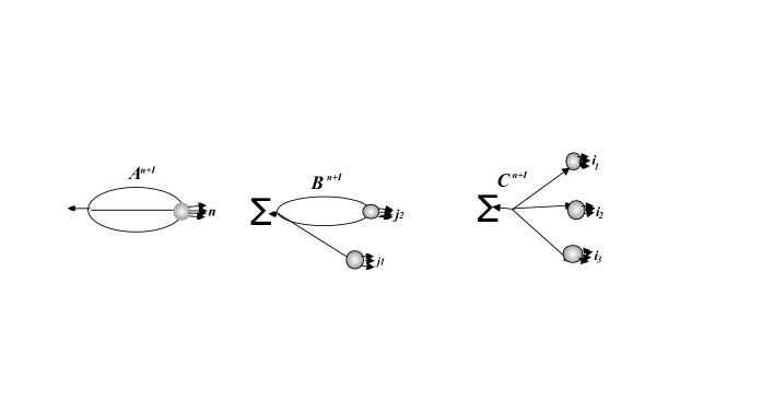
Figure 1: Graphical representation of the global terms of the $\Phi^{4}$ equations of motion

2 The dynamic system of the Green’s functions

Definition 1.1 (The $\Phi^{4}_{4}$ operations)

The infinite system of equations for the Schwinger functions (i.e. the connected, completely amputated with respect to the free propagator Green’s functions, $H=\{H^{n+1}\}_{n=2k+1,k\in{N}}$), in the Euclidean $4$-dimensional momentum space, ${\cal E}^{4n}_{(q)}$ derived from the system 1.2, 1.3, 1.4, 1.5 has the following form:

$$\begin{array}[]{l}H^{2}(q,\Lambda)=-\displaystyle{{\Lambda\over{\gamma+\rho}}}\{[N_{3}H^{4}]-aH^{2}(q,\Lambda)\Delta_{F}(q)\}+\displaystyle{{(q^{2}+m^{2})\gamma\over{\gamma+\rho}}}\\ \mbox{and}\ \ \forall\,n\geq 3,\,(q,\Lambda)\in{\cal E}^{4n}_{(q)}\times{R}^{+}\\ H^{n+1}(q,\Lambda)=\displaystyle{{1\over{\gamma+\rho}}}\{\,[A^{n+1}+B^{n+1}+C^{n+1}](q,\Lambda)+\Lambda aH^{n+1}(q,\Lambda)\}\\ \mbox{with:}\\ A^{n+1}(q,\Lambda)=-\Lambda[N^{(n+2)}_{3}H^{n+3}](q,\Lambda);\\ \\ B^{n+1}(q,\Lambda)=-3\Lambda\displaystyle{\sum_{\varpi_{n}(J)}}[N^{(j_{2})}_{2}H^{j_{2}+2}N^{(j_{1})}_{1}H^{j_{1}+1}](q,\Lambda);\\ \\ C^{n+1}(q,\Lambda)=-6\Lambda\displaystyle{\sum_{\varpi_{n}(I)}\prod_{l=1,2,3}}[N^{(i_{l})}_{1}H^{i_{l}+1}](q_{i_{l}},\Lambda);\\ a(\Lambda)=[N_{3}H^{4}]_{q^{2}+m^{2}=0};\ \ \rho(\Lambda)=-\Lambda\left[\displaystyle{\frac{\partial^{2}}{\partial q^{2}}[N_{3}^{(3)}H^{4}]}\right]_{q^{2}+m^{2}=0};\\ \\ \mbox{and}\ \ \ \gamma(\Lambda)=\left[\displaystyle{\frac{-6\Lambda\prod_{l=1,2,3}H^{2}(q_{l})\Delta_{F}(q_{l})}{H^{4}(q)}}\right]_{q=0}\end{array}$$ (1.6)

Remarks 1.1

1. Here the notations:

   $$[N^{(n+2)}_{3}H^{n+3}],\ \ \ [N^{(j_{2})}_{2}H^{j_{2}+2}N^{(j_{1})}_{1}H^{j_{1}+1}]\ \mbox{\emph{and}}\displaystyle\prod_{l=1,2,3}[N^{(i_{l})}_{1}H^{i_{l}+1}]$$

   represent the so called “$\Phi^{4}_{4}$ operations” that we introduce in the Renormalized   G-Convolution  Product $(R.G.C.P)$ context of the references [11], [12], [13]. Briefly, the two loop $\Phi^{4}_{4}$ - operation is defined by:

   $$[N^{(n+2)}_{3}H^{n+3}]=\int R^{(3)}_{G}[\ H^{n+3}\prod_{i=1,2,3}\Delta_{F}(l_{i})\ ]d^{4}k_{1}d^{4}k_{2}$$ (1.7)

   with $R^{(3)}_{G}$ being the corresponding renormalization operator for the two loops graph with bubble vertex the $H^{n+3}$ Green’s function.

   The analogous expression for the one loop $\Phi^{4}_{4}$ - operation is the following:

   $$[N^{(j_{2})}_{2}H^{j_{2}+2}][N^{(j_{1})}_{1}H^{j_{1}+1}]=H^{j_{1}+1}\Delta_{F}\int R^{(2)}_{G}[H^{j_{2}+2}\prod_{i=1,2}\Delta_{F}(l_{i})]d^{4}k$$ (1.8)

   with $R^{(2)}_{G}$, the corresponding renormalization operator for the two loops graph.

   The notation $\Delta_{F}$ indicates the free propagator, and the $\Phi^{4}_{4}$ operation $N^{(j_{1})}_{1}$ is exactly the multiplication (“trivial convolution”) by the corresponding free propagator $\displaystyle\Delta_{F}={1\over(\|q\|^{2}+m^{2})}$. Here $\|q\|^{2}$ means the Euclidean norm of the vector $q\in{\cal E}^{4n}_{(q)}$.

2. In equations 1.6 the notation $q$ in the arguments of the two-point and four-point Green’s functions is used indifferently for $q\in{\cal E}^{12}_{(q)}$ or $q\in{\cal E}^{4}_{(q)}$.

3. In the previous notations and in all that follows, ${N}$ always means the set of non negative integers and $n$ will always be an odd positive integer.

3 The “primary $\Phi$-Iteration”

1 The fixed point method

The method is based on the proof of the existence and uniqueness of the solution of the above infinite system of dynamical equations of motion verified by the Schwinger functions, following a fixed point theorem argument.

The information concerning the special features of the dynamics of four interacting fields has been obtained through an iteration at fixed coupling constant and at zero external momenta of these integral equations of motion in the two dimensional case, taking the free solution as starting point.

This is what was called the “$\Phi$-Iteration” in [2]. The exploration of the detailed organization of the different structural global terms of the $H^{n+1}_{\nu}$ functions at every order $\nu$ of what we call now the “primary $\Phi$-Iteration”, has brought forth particular properties as:

• (a) alternating signs and splitting (or factorization) properties at zero external momenta:

  $$H^{n+1}(q=0,\Lambda)=-n(n-1)\delta_{n}(\Lambda)H^{n-1}(q=0,\Lambda)[H^{2}(q=0,\Lambda)]^{2}$$ (1.9)

  with $\{\delta_{n}\}$ a bounded increasing sequence of continuous functions of $\Lambda$ and uniformly convergent to some finite positive constant $\delta_{\infty}$.

• (b) bounds at zero external momenta which in turn yield global bounds of the general form:

  $$|H^{n+1}(q,\Lambda)|\leq n\ !\ \ K^{n}\ \mbox{with $K$ a finite positive constant independent of $n$.}$$ (1.10)

These features formed a self-consistent system of conditions conserved by the “$primary\ \Phi$-Iteration”. In particular they implied precise “norms” of the sequences of the Green’s functions $H^{n+1}$:

$$\|H\|=\sup_{q,n,\Lambda}\{M_{n}^{-1}(q,\Lambda)\ \ |H^{n+1}(q,\Lambda)|\}$$ (1.11)

These norms in turn were conserved and automatically ensured the convergence of this “primary $\Phi$-Iteration” to the solution. So, in references [2] and [3] we thought about obtaining an answer to the problem by first defining a Banach space ${\cal B}_{initial}$ using the norms provided by the “primitive $\Phi$-Iteration”. and seeked a fixed point of the equations of motion inside a characteristic subset $\Phi\subset{\cal B}_{initial}$ which exactly imitated the fine structure of the $\Phi$-Iteration.

Now, taking into account the divergence of the perturbative series of a $\Phi^{4}_{2}$ model, a result that A. Jaffe [14] established several years ago, another (two-part) question immediately arises. Does the two-dimensional “$\Phi$-Iteration” generate the perturbative series exactly? If yes, then is there any contradiction between the divergence of the perturbative expansion and the convergence of the $\Phi$-Iteration? The answer is that the $\Phi$-Iteration has nothing to do with the perturbation series. The method is not a reconstruction of perturbation theory. More precisely, all terms of the $N^{th}$ order of perturbation series are included together with subsequent ones at every order $N$ of the $\Phi$-Iteration (cf.[2]a,b,). In other words the series like that of perturbation can be divergent, but a series of polynomials of the terms of the former may still be convergent. The difference between the two approaches comes from the different way in which the polynomials in $\Lambda$ are arranged and summed up in each of the two approximations. So automatically there is no contradiction if the “$\Phi$-Iteration” converges to a nontrivial solution despite the divergence of perturbation theory.

The reasons that motivated us for a study in smaller dimensions and not directly in four, were the absence of the difficulties due to the renormalization in two dimensions, and the pure combinatorial character of the problem in zero dimensions [15].

Another useful aspect of the zero dimensional case is the fact that it provides a direct way to numerically test the validity of the method [16], [17].

2 The new mapping ${\cal M}^{*}$ and the local contractivity

These “conserved norms” 1.11 lead to the convergence of the “$Primary\ \Phi$ -Iteration”. So, by introducing an appropriate Banach space ${\cal B}_{initial}$ defined by these norms and a characteristic subset $\Phi\subset{\cal B}_{initial}$ which exactly imitates the fine structure of the “Primary $\Phi$-Iteration” one expects to establish by a fixed point theorem the existence of a unique nontrivial solution inside this subset.

Unfortunately this is not the case [18]. The global terms $A^{n+1}$, $B^{n+1}$, and $C^{n+1}$, (tree terms) (with alternating signs) have identical asymptotic behavior with respect to $n$, but not what we schould expect of the corresponding $H^{n+1}$. More precisely, at every fixed value of the external momenta (precisely we proved them at zero external momenta) , we obtain:

$$A^{n+1}\mathrel{\mathop{\kern 0.0pt\sim}\limits_{n\rightarrow\infty}}(-\ \delta_{\infty})^{n-1\over 2}n!\ n^{2}$$ (1.12)

$$B^{n+1}\mathrel{\mathop{\kern 0.0pt\sim}\limits_{n\rightarrow\infty}}-(-\ \delta_{\infty})^{n-1\over 2}n!\ n^{2}$$ (1.13)

$$C^{n+1}\mathrel{\mathop{\kern 0.0pt\sim}\limits_{n\rightarrow\infty}}(-\ \delta_{\infty}^{\Lambda})^{n-1\over 2}n!\,n^{2}$$ (1.14)

As far as the behavior with respect to the external four momenta is concerned they follow the behavior of the norm functions 1.11 (i.e. the corresponding structure of the Banach space).

But, the above $n^{2}$ dependence of the global terms prevents the mapping

$${\cal M}:\,\ {\cal B}_{initial}\stackrel{{\scriptstyle\cal M}}{{\longrightarrow}}{\cal B}_{initial}$$ (1.15)

from being contractive in ${\cal B}_{initial}$, despite the convergence of the “$\Phi$-Iteration”, (thanks to the alternating signs of the global terms).

This is the reason that motivated us to define a new mapping ${\cal M}^{*}$ (equivalent to the initial mapping) given by the following equations, and which is contractive:

$$H^{n+1^{\prime}}(q,\Lambda)={\delta_{n}^{{}^{\prime}}(q,\Lambda)C^{n+1^{\prime}}(q,\Lambda)\over 3\Lambda n(n-1)}$$ (1.16)

with:

$$\delta_{n}^{{}^{\prime}}(q,\Lambda)=\frac{3\Lambda n(n-1)}{(\gamma+\rho)+D_{n}(H)-\Lambda\alpha}$$ (1.17)

and

$$D_{n}(H)={|B^{n+1}|-|A^{n+1}|\over|H^{n+1}|}$$ (1.18)

One can intuitively understand the contractivity of the new mapping ${\cal M}^{*}$ by looking at the behavior with respect to $n$ of the function $D_{n}$ (at fixed external momenta). Precisely,

$$D_{n}(H)\mathrel{\mathop{\kern 0.0pt\sim}\limits_{n\rightarrow\infty}}\displaystyle{\frac{n^{2}n\ !(\delta_{\infty})^{n-3\over 2}}{n\ !(\delta_{\infty})^{n-1\over 2}}}\mathrel{\mathop{\kern 0.0pt\sim}\limits_{n\rightarrow\infty}}\displaystyle{\frac{n^{2}}{\delta_{\infty}}}$$ (1.19)

Consequently:

$$\delta_{n}^{{}^{\prime}}(q,\Lambda)\mathrel{\mathop{\kern 0.0pt\sim}\limits_{n\rightarrow\infty}}\displaystyle{\frac{\delta_{\infty}n(n-1)}{n^{2}}}\mathrel{\mathop{\kern 0.0pt\sim}\limits_{n\rightarrow\infty}}\delta_{\infty}$$ (1.20)

By this last argument one can show not only the conservation of the norms but also the contractivity of the “new mapping” ${\cal M}^{*}$ to a fixed point inside a characteristic subset $\Phi\subset{\cal B}_{initial}$, under a sufficient condition of the following type imposed on the renormalized coupling constant:

$$0\leq\Lambda\leq\Lambda_{0}$$ (1.21)

In an equivalent way, this result implies the existence and uniqueness of a nontrivial solution (even in four dimensions), of the system. Under the condition 1.21, this solution lies in a neighborhood of a precise point-sequence of the appropriate subset $\Phi\subset{\cal B}$, the so-called fundamental sequence $\{H_{T0}\}$.

Consequently, the construction of this non perturbative solution can be obtained by the iteration of the mapping ${\cal M}^{*}$ inside $\Phi\subset{\cal B}$ starting from the corresponding, to every dimension, fundamental sequence $\{H_{T0}\}$. So, this solution verifies automatically, the“alternating signs” and “splitting” properties at every value of the external momenta, analyticity properties together with the physical conditions imposed on $H^{2}$- and $H^{4}$ - Green’s functions for the definition of the renormalization parameters.

The essential results of the method in 4 dimensions are the following:

1. The proof of the “alternating signs” and “splitting” properties at every value of the external momenta (and not only at zero external momenta as we had originally established in the “primary $\Phi$-Iteration”).

2. The proof of specific asymptotic increase properties with respect to the four dimensional external momenta of the renormalized Green’s functions, in particular the powers of $q^{2}\log(q^{2})^{k}$ which dominate the $H^{2}$-point function’s behaviour.

3. The proof of A.Q.F.T. properties in complex Minkowski space.

4. The proof of the existence and uniqueness of solution of the system 1.6 obtained as a limit of a (new) renormalized iteration procedure (the so called “$\Phi^{4}_{4}$- iteration") or in other words as a fixed point of a locally contractive mapping in the neighborhood of a precise “tree type” sequence.

4 Planning of the paper

The paper is organized as follows:

1. In section $2$ we introduce the general vector space ${\cal B}$, the tree type sequences, and the Renormalized $\Phi$ Convolutions (R.$\Phi$.C.) - Green’s functions using as building block one of the tree type sequences the ‘‘fundamental tree type sequence” $H_{T0}$. (cf.def. 2.5 )
   Then we define the “renormalized subspace” ${\cal B}_{R}\subset{\cal B}$ which (being provided with the appropriate norm) is a Banach space.

2. In section $3$

   • We introduce a particular subset $\Phi_{R}\subset{\cal B}_{R}$ characterized by the detailed bounds, signs, splitting properties, consistent definitions of the renormalization parameters $a,\ \rho,\mbox{and}\ \gamma$, together with the analyticity properties of general n-point functions (in the A.Q.F.T. framework). The non triviality of $\Phi_{R}\subset{\cal B}_{R}$ is established by proving that $H_{T0}\in\Phi_{R}$.

   • We define the Generalized Renormalized $\Phi$- Convolutions (G.R.$\Phi$.C.) and the new mapping ${\cal M}^{*}$ on ${\cal B}_{R}$.

   • By successive application of ${\cal M}^{*}$ on $H_{T0}$ a $\Phi_{4}^{4}$- iteration is defined which preserves the good properties of $H_{T0}$ and automatically establishes the stability of a neighbourhood of $\Phi_{R}$ under ${\cal M}^{*}$.

3. Section $4$ contains the construction of the solution: the local contractivity of the mapping ${\cal M}^{*}$ inside a precise closed ball in ${\cal B}_{R},\ \ {\cal S}(H_{T0},r_{0})\subset\Phi_{R}$.

4. In the Appendices we present the necessary proofs of the theorems stated in sections $3$ and $4$.

2 The vector space ${\cal B}$ - the“splitting sequences”
the “tree type sequences” and the Banach space ${\cal B}_{R}$

The fundamental difference between two and four (or three) dimensions is the divergence in the latter case of a finite number of $\Phi-Convolutions$ for every fixed integer $n=2k+1,\ \ k\in{{N}}$. Therefore, it has been necessary to introduce the precise definition of the renormalization operations and choose a more specific space of Green’s functions sequences in the A.Q.F.T. framework.

To this purpose, we introduce the basic elements of this space, the so-called tree type sequences $H_{T}$, and from a particular choice of one of them, we recursively define the Renormalized $\Phi-Convolutions$ $(R.F.C)$. For the detailed definitions and statements concerning the recursive procedure of the renormalization, we refer the reader to the references [11] [12][13].

Apart from a brief reminder of certain crucial properties, we apply the results of these papers without any detailed description.

1 The space ${\cal B}$ - the“splitting sequences”

Definition 2.1

The space ${\cal B}$

We define the vector space ${\cal B}$ of the sequences $H=\{H^{n+1}\}_{{n=2k+1;}\atop{k\in{N}}}$ as follows:

For every $n$ the function $H^{n+1}$ belongs to the space $C^{\infty}({\cal E}^{4n}_{(q)}\times{{R}}^{+})$ of continuously differentiable real numerical functions of the set $(q,\Lambda)$ of $4n+1$ real independent variables and verifies the following properties. There exists a finite positive constant $C_{n}$, such that the following bounds hold:

$$\begin{array}[]{l}\forall\ (q,\Lambda)\in({\cal E}^{4}_{(q)}\times{{R}}^{+})\\ |H^{2}(q,\Lambda)|\leq C_{1}[(\|q\|^{2}+m^{2})^{(1+\pi^{2}/18)}]\end{array}$$ (2.22)

and $\forall\,n=2k+1\,\quad k\in{N}^{*},\ (q,\Lambda)\in({\cal E}^{4n}_{(q)}\times{{R}}^{+})$

$$|H^{n+1}(q,\Lambda)|\leq n!C_{n}[(\|q\|^{2}+m^{2})^{(1+\pi^{2}/18)}]^{n}$$ (2.23)

Here the notation $\|q\|=\displaystyle{\sqrt{\sum_{i=1}^{n}q_{i}^{2}}}$ means the Euclidean norm of the vector $q\in{\cal E}^{4n}_{(q)}$. In the following we often use the equivalent notation: $\|q\|^{2}=q^{2}$.

Definition 2.2

The "splitting sequences" $\delta\in\mathcal{B}$

We introduce the particular class $\mathcal{D}\subset\mathcal{B}$ of the so-called “splitting sequences” $\delta=\{\delta_{n}(q,\Lambda)\}_{n=2k+1\ k\in{N}}\in\mathcal{B}$.

There exists a finite positive constant $C_{0}$ such that the corresponding bounds (2.23) take the following form:

$$\begin{array}[]{l}\forall\,n=2k+1\quad k\in{N}^{*}\\ 0\ <\delta_{n}(q,\Lambda)\leq C_{0}\quad\ \forall(q,\Lambda)\in{\cal E}^{4n}_{(q)}\times{R}^{+}.\end{array}$$ (2.24)

2 The "tree type sequences" $H_{T}$

Definition 2.3

We define the following class of sequences $H_{T}$ associated with a given splitting sequence $\delta\in\mathcal{D}$:

$$\begin{array}[]{l}\ \ \ \forall\ (q,\Lambda)\ \in({\cal E}^{4n}\times{R}^{+*})\\ \\ H_{T}^{2}(q,\Lambda)=(q^{2}+m^{2})(b_{0}(\Lambda)+b_{1}(\Lambda)(q^{2}+m^{2})^{(1+\pi^{2}/18)}\\ \mbox{(here $b_{0}$ and $b_{1}$ are in general continuous bounded positive functions of $\Lambda$)}\\ H_{T}^{4}(q,\Lambda)=\ -\delta_{3}(q,\Lambda)\displaystyle{\prod_{j=1,2,3}}H_{T}^{2}(q_{{j}},\Lambda)\Delta_{F}(q_{{j}})\\ \mbox{and}\quad\forall\,n\geq 5\\ H_{T}^{n+1}(q,\Lambda)=-\displaystyle{\frac{\delta_{n}(q,\Lambda)}{n(n-1)}\sum_{\varpi_{n}(I)}\prod_{j=1,2,3}H_{T}^{i_{j}+1}(q_{i_{j}},\Lambda)}\Delta_{F}(q_{i_{j}})\end{array}$$ (2.25)

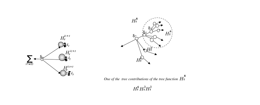
Figure 2: Graphical representation of a general tree function $H_{T}^{n+1}$, and a zoom on the bubble vertices of one of the tree terms of the $H_{T}^{8}$ function.

We call these sequences $H_{T}$ (resp. every $H_{T}^{n+1}$) the "tree type sequences" (res. the tree functions $H_{T}^{n+1}$). For every $n\geq 5$ the graphical representation of every $H_{T}^{n+1}$ is a finite sum of “tree graphs”, with a four point bubble vertex associated with the corresponding $\delta_{n}(q,\Lambda)$ connected by three simple free propagators $\Delta_{F}(q_{i_{j}})$ to three “bubble vertices”. These bubbles represent each one of the three tree functions $H_{T}^{i_{j}+1}$ of the corresponding partition in the sum (cf.fig.2).

1 Particular splitting sequences-Reminders

In [15] we introduced the following particular splitting sequences for the zero dimensional problem.

Definition 2.4

1. The upper and lower bounds - splitting sequences

   $$\begin{array}[]{l}\ \ \ \ \ \delta_{3,max}(\Lambda)=\displaystyle{\frac{6\Lambda}{\gamma_{0}+\rho_{0}+\Lambda|a_{0}|+6d_{0}}};\qquad\delta_{3,min}(\Lambda)=\displaystyle{{6\Lambda\over 1+9\Lambda(1+6\Lambda^{2})}}\\ \mbox{and}\ \ \forall n\geq 5\\ \delta_{n,max}(\Lambda)=\displaystyle{\frac{3\Lambda n(n-1)}{\gamma_{0}+\rho_{0}+\Lambda|a_{0}|+n(n-1)d_{0}}}\\ \mbox{with:}\\ \gamma_{0}=1,\ \quad a_{0}=-\delta_{3,min}[N_{3}\tilde{]}_{q^{2}+m^{2}=0};\quad\rho_{0}=\Lambda\delta_{3,min}[\displaystyle{\frac{\partial}{\partial q^{2}}[N_{3}\tilde{]}]_{q^{2}+m^{2}=0}}\\ \mbox{and}\\ \delta_{n,min}(\Lambda)=\displaystyle{{3\Lambda\ n(n-1)\over\gamma_{max}+\rho_{max}+\Lambda|a_{max}|+3\Lambda n\ (n-1)}}\\ \mbox{with}\\ \gamma_{max}=1+9\Lambda(1+6\Lambda^{2}),\quad\rho_{max}=6\Lambda^{2}\displaystyle{\frac{\partial}{\partial q^{2}}}[N_{3}\tilde{]}_{q^{2}+m^{2}=0}\ \ \ \mbox{and}\\ |a_{max}|=6\Lambda[N_{3}\tilde{]}_{q^{2}+m^{2}=0}\\ \end{array}$$ (2.26)

   Remarks 2.1

   • Notice that for the constant $d_{0}$ appearing in the definition of $\delta_{n,max}$ we put $d_{0}=3\Lambda 10^{-2}$ that is precisely the value we determined and used in [15] for the zero dimensional case.

   • For the $\delta_{n,min}$’s in 4-dimensions we need to use the maximal values of the renormalization constants obtained directly by the definitions 1.6.

   • Concerning the $\delta_{n,max}$’s in 4-dimensions we need to use the minimal values of the renormalization constants $\gamma_{0}$, $\rho_{0}$, and $a_{0}$ (cf. def.2.5).

2. The solution of the zero dimensional mapping ${\cal M}^{*}_{0}$.

   In [15] we proved the existence and uniqueness of the splitting sequence $\{\delta_{n0}\}$-solution of the zero dimensional mapping ${\mathcal{M}}^{*}_{0}$ defined as follows: ${\cal M^{*}}:\,\Phi_{0}\stackrel{{\scriptstyle\cal M^{*}}}{{\longrightarrow}}{\cal B}_{0}$:

   $$\begin{array}[]{l}H^{2^{\prime}}(\Lambda)=1-\Lambda H^{4}(\Lambda)\\ H^{4^{\prime}}(\Lambda)=-\delta_{3}^{\prime}(\Lambda)[H^{2^{\prime}}]^{3}\quad\hbox{with}\quad\displaystyle{\delta_{3}^{{}^{\prime}}(\Lambda)=\frac{6\Lambda}{1+\ D_{3}}}\\ \mbox{and}\quad D_{3}=6\Lambda H^{2}\left(3/2-\frac{|H^{6}|}{6|H^{4}||H^{2}|}\right);\\ \mbox{moreover:}\\ \qquad\forall\ n\geq 5\qquad H^{n+1^{\prime}}(\Lambda)=\displaystyle{\delta_{n}^{{}^{\prime}}(\Lambda)C^{n+1^{\prime}}\over\displaystyle 3\Lambda n(n-1)}\\ \mbox{Here:}\qquad\delta_{n}^{{}^{\prime}}(\Lambda)=\displaystyle{\frac{3\Lambda n(n-1)}{1+D_{n}(H)}}\\ \mbox{ with:}\quad D_{n}(H)=\displaystyle{{|B^{n+1}|-|A^{n+1}|\over|H^{n+1}|}}\end{array}$$ (2.27)

2 The “fundamental tree type sequence” $H_{T0}$

For further purposes, we introduce the particular tree type sequence $H_{T0}$ that we shall call “fundamental” defined as follows:

Definition 2.5

$$\begin{array}[]{l}\gamma_{0}=1\\ a_{0}=-\delta_{3,min}[N_{3}\tilde{]}_{(q^{2}+m^{2})=0};\\ \\ \rho_{0}=\Lambda\delta_{3,min}[\displaystyle{\frac{\partial}{\partial q^{2}}[N_{3}\tilde{]}]_{(q^{2}+m^{2})=0}}\\ \\ \mbox{(Reminder: $\quad\delta_{3,min}=\displaystyle{\frac{6\Lambda}{1+9\Lambda(1+6\Lambda^{2})}}$)}\\ \forall(q,\Lambda)\in(\mathcal{E}_{(q)}^{4}\times{R}^{+*})\\ H_{T0}^{2}=(q^{2}+m^{2})(1+\delta_{10}(q,\Lambda)\Delta_{F})\\ \mbox{with}\quad\delta_{10}(q,\Lambda)\Delta_{F}=\displaystyle{\frac{-\rho_{0}+\Lambda\delta_{3,min}([N_{3}\tilde{]}-[N_{3}\tilde{]}_{(q^{2}+m^{2})=0})\Delta_{F}}{1+\rho_{0}}}\\ \forall(q,\Lambda)\in(\mathcal{E}_{(q)}^{12}\times{R}^{+*})\quad\ H_{T0}^{4}=-\delta_{3,min}(\Lambda)\displaystyle{\prod_{l=1,2,3}H^{2}_{T0}(q_{l})\Delta_{F}(q_{l})}\\ \\ \mbox{and for every $n\geq 5$ and $\forall\ (q,\Lambda)\in(\mathcal{E}_{(q)}^{4n}\times{R}^{+*})$}\\ H^{n+1}_{T0}(q,\Lambda)=\displaystyle{{\delta_{n,min}(\Lambda)C^{n+1}_{T0}(q,\Lambda)\over 3\Lambda n(n-1)}};\\ \mbox{where}:\\ C^{n+1}_{T0}(\Lambda)=-6\Lambda\displaystyle{\sum_{\varpi_{n}(I)}{n\ !\over i_{1}!i_{2}!i_{3}!\ \sigma_{sym}(I)}\prod_{l=1,2,3}H^{i_{l}+1}_{T0}\Delta_{F}(q_{i_{l}})}\\ \mbox{and\ $\{\delta_{n,min}\}_{n\geq 3}$\ is the splitting sequence of definition \ref{def. 2.4}.}\end{array}$$ (2.28)

3 The Renormalized $\Phi$-Convolutions

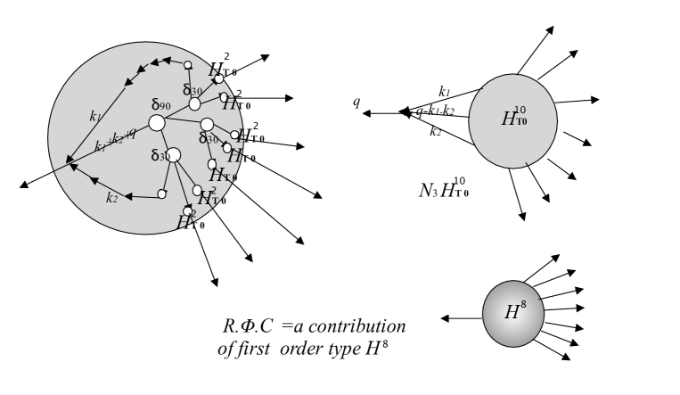
Figure 3: Graphical representation of a “first order R. $\Phi$. C.” - $H_{\nu=1}^{8}$-point function, coming from applying once $[N^{(9)}_{3}]-\Phi_{4}^{4}$ operation, on the “zero order” tree contribution of the tree function $H_{T0}^{10}$ .

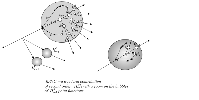
Figure 4: Graphical representation of a tree type $\Phi^{4}$ operation of order $\nu=2$ for the first term $C^{10}_{\nu=2}$ of $H_{\nu=2}^{1}0$-point function, by using the bubble-vertex of figure 3 of $H_{\nu=1}^{8}$-point function and the bubble-vertices $H_{\nu=1}^{2}$-point functions (coming from a $\Phi_{4}^{4}$ on $H_{T0}^{4}$-point function)

Figure 5: Graphical representation of $H^{8}$-type point bubble-function (third order $H_{\nu=3}^{8}$-point function R. $\Phi$. C.), obtained after three successive applications of $\Phi_{4}^{4}$ operations on the “zero order” tree contribution of the tree function $H_{T0}^{10}$. It could constitute a bubble vertex of a tree contribution $H^{8}H^{2}H^{2}$ of third order R. $\Phi$. C. $H_{T0}^{10}$. Here $L=5$ and $\mathcal{L}=12$ so that 20-24=-4 is the asymptotic Weinberg indicatrix of an $H^{8}$ point function

Definition 2.6

Using the previously defined fundamental tree type sequence $H_{T0}$ we recurrently construct the infinite family of the so-called Renormalized $\Phi$-convolutions as follows:

We successively apply in an arbitrary way the $\Phi^{4}_{4}$-operations (defining the mapping $\mathcal{M}$ by definition 1.6); (cf. example fig.3 and fig 5).

At a certain order $\nu$ of this iteration we consider the corresponding result from an arbitrary $H_{T0}^{n+1}$ tree function. Graphically it is the sum of tree type functions with“bubbles”, the corresponding images coming from successive applications of the $\Phi^{4}_{4}$ operations on the vertices of every tree contribution of the original $H_{T0}^{n+1}$ tree function.

We denote by $\Phi_{n}^{\bar{n}(\nu)}(q,\Lambda)$ such a bubble (with $\bar{n}(\nu)+1$ external lines), and call it the Renormalized $\Phi$-Convolution (R.$\Phi$.C) associated with the $H_{T0}^{n+1}$ tree-type function.

Every $\Phi_{n}^{\bar{n}(\nu)}(q,\Lambda)$, depends on the set $q=(q_{1},\cdots,q_{\bar{n}(\nu)})(q\in\mathcal{E}_{(q)}^{4\bar{n}(\nu)}$) of the (remaining after the integrations) external independent momenta. It constitutes a candidate bubble vertex for new tree type sequence in $\cal B$ (cf. figures  4 and 5).

Using the general prescription of renormalization of [11] we introduce the renormalization operator at every step of the above recursive construction. More precisely suppose that $\Phi_{n}^{\bar{n}(\nu)}(q,\Lambda)$ has been already well defined and we want to construct the newly composed convolution $[N_{3}^{(\bar{n}(\nu)+2)}\Phi_{n}^{\bar{n}(\nu)}(q,\Lambda)]$. We define:

$$[N_{3}^{(\bar{n}(\nu)+2)}\Phi_{n}^{\bar{n}(\nu)}(q,\Lambda)]\equiv\int R_{G}^{(3)}[\Phi_{n}^{\bar{n}(\nu)}(q,\Lambda)\prod_{k=1,2,3}\Delta_{F}(\ell_{k})]\ d^{4L}k$$ (2.29)

Here $G$ is the total graph representing the R.$\Phi$.C. $[N_{3}^{(n^{\prime}=\bar{n}(\nu)+2)}\Phi_{n^{\prime}}^{\bar{n}}]$ and $R_{G}^{(3)}$ the renormalization operator. For the precise momentum assignment (following [11]) we consider the product vector space defined by: $\mathcal{E}_{(q,k)}^{4N}\equiv\mathcal{E}_{(q)}^{4n}\otimes E_{(k)}^{4L}$ with $N=n+L$. We associate these notations with the set of external independent $(q)$ (resp. internal $(k)$ or integration) variables of the given R.$\Phi$.C. $[N_{3}^{(n^{\prime})}\Phi_{n^{\prime}}^{\bar{n}}]$. The integer $L$ indicates the number of independent loops of $G$ (i.e. the integration variables $k\in E_{(k)}^{4L}$ of the R.$\Phi$.C.). We also use the notation $\mathcal{L}$ for the set of all internal lines of $G$. The non renormalized integrand $I_{G}(q,k)$, is simply the product of the vertex functions (bubble vertices) and free propagators (simple internal lines) involved in the initial R.$\Phi$.C, $\Phi_{n^{\prime}}^{\bar{n}}$ and the product of free propagators associated with $N_{3}^{(n^{\prime})}$ so,

$$I_{G}(q,k)=\prod_{v_{j}}H_{T}^{n_{j}+1}\prod_{i\in\mathcal{L}}\Delta_{F}(\ell_{i})\prod_{k=1,2,3}\Delta_{F}(\ell_{k}).$$ (2.30)

The argument $\ell_{i}$, of every free propagator means the total momentum carried by the corresponding internal line $i\in\mathcal{L}$ associated with the linear application $\lambda_{i}$:

$$(q,k)\stackrel{{\scriptstyle\lambda_{i}}}{{\leftrightarrow}}\ell_{i}(q,k)$$ (2.31)

The precise form of the function $\ell_{i}(q,k)$ is given by the conditions of energy momentum conservation imposed on the momentum assignement at every vertex of $G$. A definition analogous to that of 2.30 holds for the non renormalized integrand associated with every subgraph $\gamma$ of $G$.

Following [11], the abbreviated notation for the renormalized integrand means precisely:

$$R_{G}^{(3)}\left[\Phi_{n^{\prime}}^{\bar{n}}\prod_{k}\Delta_{F}(\ell_{k})\right]=\sum_{U_{\mathcal{F}(G)}}(1-t^{d(G)})Y_{G}^{(3)}(U_{\mathcal{F}})$$ (2.32)

The sum $\displaystyle{\sum_{U_{\mathcal{F}(G)}}}$ extends over all complete forests $U_{\mathcal{F}}$ of $G$ (with respect to a nested set $\mathcal{S}$ of subspaces $S\subset E_{(k)}^{4L}$ containing nontrivial renormalization parts $\gamma$ subgraphs of $G$. The functions $Y_{G}^{(3)}(U_{\mathcal{F}})$ (and the corresponding, $Y_{\gamma}^{(3)}(U_{\mathcal{F}})$ for every $\gamma\in U_{\mathcal{F}}$) are also recursively defined in the ref.[11]. Notice that the degree of Taylor operators $d(G)$ (resp. $d(\gamma)$) coincides with the superficial degree of divergence of the graph $G$ (resp. of $\gamma$) and below (cf. proposition 2.1 ) we shall give precise upper bounds for these numbers in terms of the asymptotic indices of the tree functions. In an analogous way we define the renormalized $\Phi^{4}$ operation $[N_{2}^{(n^{\prime}-1)}\Phi_{n^{\prime}}^{\bar{n}}(q,\Lambda)]$.

For the convergence proof of the R.$\Phi$.C’s we shall use Weinberg’s criterion of convergence applied to a certain class of Weinberg functions.

A class of Weinberg functions (cf.[25], [11]) $f\in C^{\infty}(\mathcal{E}_{(q)}^{4n})$ is denoted by $\mathcal{A}_{4n}^{(\alpha,\beta)}$ and is characterized by two bounded real valued functions $\alpha(S),\ \beta(S)$, on the set of all linear subspaces $S\subset\mathcal{E}_{(q)}^{4n}$, which are called the "asymptotic indicatrices".

In [11] particular classes of Weinberg functions have been introduced (the classes of admissible Weinberg functions) and they have played a fundamental role for the convergence proof and good asymptotic behavior of the renormalized convolutions by an extension of the  B.P.H.Z [26] renormalization procedure.

The study in [11] concerned the most general convolutions (the so-called $G$-convolutions) in a space of arbitrar dimensions space. The corresponding graphs were defined by bubble vertices $v$ (resp. complete internal lines) associated with general $H^{n_{v}}$ point functions (resp. with general $H^{2}$-point functions) satisfying all appropriate A.Q.F.T. properties.

Under the assumption that the general $H^{n_{v}},\ H^{2}$ - point functions belong to the classes of symbols of pseudodifferential operators $\sum_{4(n_{v}-1)}^{\mu_{v}},\ \sum_{4}^{\mu_{i}}$ it has been proven (cf. theorem 4.1 of [11]) that for every such $G$-convolution, the corresponding renormalized integrand belongs to the class of Weinberg functions with the appropriate asymptotic indices. So the Weinberg’s criterion of convergence is verified.

Moreover in [12] (resp. in [27]) the asymptotic behavior with respect to the powers of external momenta (resp. with respect to powers of logarithms also) has been established for the $G$-convolutions, by using the same prescription of renormalization. We shall use here the definition of projection of a subspace $S$ of $\mathcal{E}_{(q,k)}^{4N}$ onto $E_{(k)}^{4L}$ established in [11] and [27] concerning the classes of symbols and the classes of admissible Weinberg functions which have been denoted by $\mathcal{A}_{4N}^{(\alpha,\beta,\sigma,\omega)}$.

We do not give here the corresponding precise definitions; we simply notice that $(\sigma,\omega)$ is a couple of sets of such subspaces in $E_{(k)}^{4L}$ and $E_{(q,k)}^{4N}$ respectively, where under differentiation the corresponding asymptotic indicatrices $\alpha,\beta$ decrease. We also recall the notation $\pi(S)$ for the canonical projection of a subspace $S$ of $E_{(q,k)}^{4N}$ onto $E_{(k)}^{4L}$.

Before giving the main theorem for the convergence of every R.$\Phi$.C we show an auxiliary statement. Let us start with some useful notations and definitions.

Definition 2.7

We denote by $q_{T}^{j}$ the set of independent momenta of the tree function $H_{T}^{n_{j}+1}$ associated with the vertex $v_{j}$ of a given graph $G$. We define the following linear mapping

$$\lambda_{\nu_{j}}:\qquad(q,k)\stackrel{{\scriptstyle\lambda_{\nu_{j}}}}{{\leftrightarrow}}q_{T}^{j}(q,k)$$ (2.33)

We notice that, as previously, the function $q_{T}^{j}(q,k)$ is precisely defined by the momentum assignment, following the prescription of [11], when all constraints of energy momentum conservation at each vertex $\nu_{j}$ of $G$ are taken into account. We then state the following:

Proposition 2.1

Given a R.$\Phi$.C and the associated $G$-graph the following properties hold:

a) Every vertex function $H^{n_{j}+1}$ associated with the bubble vertex $v_{j}$ of $G$, belongs to the class $\mathcal{A}_{4N}^{(\alpha_{v_{j}}\beta_{v_{j}},\sigma_{v_{j}},\omega_{v_{j}})}$ of admissible Weinberg functions. The sets $\sigma_{v_{j}},\ \omega_{v_{j}}$ are defined by:

$$\sigma_{v_{j}}=\{S\subset E_{(k)}^{4L}:\quad S\not\subset\mathcal{K}er\lambda_{v_{j}}\}\ ;$$ (2.34)

$$\omega_{v_{j}}=\{S\subset E_{(k)}^{4N}:\quad\pi(S)\in\sigma_{v_{j}}\}.$$ (2.35)

For every $S\subset\mathcal{E}_{(q,k)}^{4N}$ the corresponding asymptotic indicatrices are given by:

$$\alpha_{v_{j}}(S)=\left\{\begin{array}[]{rl}-(n_{j}-3),&\mbox{if }\ S\not\subset\mathcal{K}er\ \lambda_{v_{j}}\\ 0&\mbox{if }\ S\subset\mathcal{K}er\ \lambda_{v_{j}}\end{array}\right\}$$ (2.36)

$$\beta_{v_{j}}(S)=\left\{\begin{array}[]{l}2\nu_{(n_{j})}\ \mbox{if}\ S\not\subset\mathcal{K}er\ \lambda_{v_{j}}\\ 0\ \ \mbox{if }\ S\subset\mathcal{K}er\ \lambda_{v_{j}}\\ \mbox{ and $\nu_{(n_{j})}\in{N}$ arbitrary large depending on $n_{j}$}\end{array}\right\}$$ (2.37)

b) The non renormalized integrand $I_{G}(q,k)$ associated with $G$ (cf. equation 2.30 of definition 2.6) belongs to the class of admissible Weinberg functions

$\mathcal{A}_{4N}^{(\alpha_{G},\beta_{G},\sigma_{G},\omega_{G})}$ characterized by the following sets and indices:

$$\sigma_{G}=\displaystyle{\bigcap_{i\in\mathcal{L}}\sigma_{i}\bigcap_{v_{j}}\sigma_{v_{j}}}$$ (2.38)

$$\omega_{G}=\{S\subset\mathcal{S}_{(q,k)}^{4N}:\ S\not\subset\mathcal{K}er\ \lambda_{i}\quad\forall\;i\in\mathcal{L},\ \pi(S)\in\sigma_{G}\}$$ (2.39)

and for every $S\subset\mathcal{E}_{(q,k)}^{4N}$ :

$$\alpha_{G}(S)=\sum_{v_{j}}\alpha_{v_{j}}(S)+\sum_{i\in\mathcal{L}}\mu_{i}(S)$$ (2.40)

Here $\forall\;i\in\mathcal{L}$,

$$\mu_{i}(S)=\{-2\mbox{ if }S\not\subset\mathcal{K}er\ \lambda_{i}\;\ \mbox{ and }0\mbox{ if }S\subset\mathcal{K}er\ \lambda_{i}\}$$ (2.41)

and

$$\beta_{G}(S)=\sum_{v_{j}}\beta_{v_{j}}(S)$$ (2.42)

c) Analogous result holds for the non renormalized integrand associated with every subgraph $\gamma$ of $G$.

d) The degree $d(G)$ (resp. $d(\gamma)$) of the Taylor operators associated with $G$ (resp. with $\gamma$) in formulas (2.45) is bounded as follows:

$$d(G)\leq 2\ ;\mbox{ (resp. }d(\gamma)\leq 2).$$ (2.43)

Proof of proposition 2.1

The proof is obtained by application of the previous definitions (in particular the definitions of the admissible classes of Weinberg ) and is a direct consequence of [11] and [27]. Notice that for every $n\geq 3$ the function $\delta_{n}(q,\Lambda)$ belongs to the class of Weinberg functions $\mathcal{A}_{4N}^{(0,0,\sigma_{\nu j},\omega_{\nu j})}$.

We use the notation $|\mathcal{L}|$ for the total number of internal lines of $G$ we have :

$$d(G)=-2|\mathcal{L}|+\max_{S}\sum_{\nu_{j}}\alpha_{v_{j}}(S)+4L\leq 2\ \quad\blacksquare$$ (2.44)

Taking into account the above results we notice that the conditions for the non renormalized integrand of $G$ established in [11] are all verified. So we are allowed to apply directly the corresponding theorems of refs. [11], [12] and [27] in order to obtain the following result that we present without proof :

Theorem 2.1

Every R.$\Phi$.C. $\Phi_{n}^{\bar{n}}(q,\Lambda),\ (q\in\mathcal{E}_{(q)}^{4n}$) with $n$ external independent variables and $L$ integration variables $k\in E_{(k)}^{4L}$, (with $\Lambda$ a fixed real positive number) verifies the following properties:

• Defined as an integral of $k\in E_{(k)}^{4L}$, it is absolutely convergent and it belongs to the class $\mathcal{A}_{4n}^{(\alpha_{n},\beta_{n})}$ of Weinberg functions with the following precise asymptotic indicatrices:

  $$\begin{array}[]{l}\forall S\subset\mathcal{E}_{(q)}^{4n}:\\ \alpha_{n}(S)=d(G)\quad;\quad\beta_{n}(S)=\tilde{\nu}_{(n)}\\ \mbox{with $\tilde{\nu}$ an arbitrary big natural number depending on n }\end{array}$$ (2.45)

• It satisfies Euclidean invariance and all linear axiomatic field theory properties of a general $n+1$-point function in complex Minkowski space.

4 The Generalized Renormalized $\Phi$- Convolution (G.R.$\Phi$.C.)

Definition 2.8

A Generalized R.$\Phi$.C. (G.R.$\Phi$.C.) is defined as the image of different $\Phi_{4}^{4}$ operations on an arbitrary finite sum of R.$\Phi$.C’s. The corresponding to a G.R.$\Phi$.C, $G_{\Phi}$ graph contains sums of disconnected graphs associated to each one of the connected components R.$\Phi$.C’s.

The renormalization operator $R_{G}$ corresponding to the operations $N_{3}^{(n)}$ and $N_{2}^{(n-1)}$ respectively is defined as a consistent extension of the scheme presented previously for the R.$\Phi$.C’s. More precisely, the renormalized integrand (analog of formula 2.32 ) corresponding to the convolution $[N_{3}^{(r)}\Phi_{(r)}^{(n)}]$ reads:

$$R_{G_{\Phi}}^{(3)}[\Phi_{(r)}^{(n)}(H)\prod_{k}\Delta_{F}(\ell_{k})]=\sum_{U_{\mathcal{F}}(G_{\Phi}(H))}(1-t^{d(G_{\Phi})})Y_{G_{\Phi}}^{(3)}(U_{\mathcal{F}}(H))$$ (2.46)

Here, the argument $H$ means that the summation is multiple because the fine structure of the corresponding $H\in\mathcal{B}$ must be taken into account and every $H^{n_{j}+1}$-function associated with the bubble vertex $v_{j}$ of $G_{\Phi}$, must be expanded in its terms R.$\Phi$.C’s (cf. def.2.6).

In other words, the total graph $G_{\Phi}(H)$ is, in fact, a sum of disconnected graphs $G^{*}$ coming from the expansion of all bubble vertices in their disconnected components graphs $G$ associated with the R.$\Phi$.C’s involved in the definition of the corresponding $H^{n_{j}+1}$’s. Therefore the sum in 2.46 contains all possible nontrivial individual forests of every such component $G^{*}$. Notice that now, the associated vertex functions are not in general tree functions. For simplicity we keep the same mode of notation for the number $n$ of the initial function $H^{n+1}$ (superscript) and respectively the number $r$ of external independent variables (subscript) as in the definition 2.6 of the R.$\Phi$.C’s.

5 The Banach space $\mathcal{B}_{R}\subset\mathcal{B}$

Definition 2.9

We say that a sequence $H\in\mathcal{B}$ belongs to the linear subspace $\mathcal{B}_{R}\subset\mathcal{B}$, if   $\forall\,n=2k+1,\ k\in{N}$ the corresponding $H^{n+1}$ function is a (G.R.$\Phi$.C.) in the sense of definition 2.10.

Definition 2.10 ($\mathcal{B}_{R}\subset\mathcal{B}$ a Banach space)

We introduce the following positive mapping on $\mathcal{B}_{R}$

$$\mathcal{N}:\ \ \mathcal{B}_{R}\to{R}^{+}$$

$H\mapsto\|H\|$ Here

$$\begin{array}[]{l}H\mapsto\|H\|\ \ \ \mbox{where}\ \ \ \|H\|=\displaystyle{\sup_{\Lambda}}\left\{\displaystyle{\sup_{n,q}}\left\{\displaystyle{\frac{|H^{n+1}|}{M_{n}}};\displaystyle{\frac{|\frac{\partial^{(0,1)}}{\partial q^{2}}|N_{3}H^{4}|}{\hat{M}_{3}^{(0,1)}}};\displaystyle{\frac{|N_{2}H^{n+1}|}{\hat{M}_{(n,2)}};\frac{|\gamma|}{{\cal N}_{\gamma}}}\right\}\right\}\\ \mbox{where:}\quad\forall\ (q,\Lambda)\in\mathcal{E}_{(q)}^{4n}\times{R}^{+*}\\ M_{1}(q)=\gamma_{max}(q^{2}+m^{2})(1+6(q^{2}+m^{2})^{\pi^{2}/54})\\ {\cal N}_{\gamma}=\gamma_{max}\displaystyle{\prod_{i=1}^{3}M_{1}(q_{i})\Delta_{F}(q_{i})|_{q^{2}=0}}\\ \gamma_{max}=1+9\Lambda(1+6\Lambda^{2})\\ M_{3}(q)=6\Lambda\displaystyle{\prod_{i=1}^{3}M_{1}(q_{i})\Delta_{F}(q_{i})}\\ \hat{M}_{3}^{(0,1)}(\Lambda)=6\Lambda\ \displaystyle{\sup_{q}}\left[|\displaystyle{\frac{\partial}{\partial q^{2}}}[N_{3}\tilde{I}_{1,3}]|M_{1};\ |[N_{3}\tilde{I}_{1,3}]|M_{1}\right]\\ \mbox{with}\quad\tilde{I}_{1,3}=\displaystyle{\prod_{i=1}^{2}M_{1}(k_{i})[\Delta_{F}(k_{i})]^{2}\Delta_{F}(k_{1}+k_{2}+q)}\\ \mbox{(cf. also \ref{2.30} , \ref{2.32}) \ \ and figures\ \ref{fig.H102treecontrib.pdf} )}\\ \mbox{by analogy}\quad\hat{M}_{(3,2)}=6\Lambda[N_{2}^{(3)}\tilde{I}_{1,2}]\displaystyle{\prod_{i=2}^{3}M_{1}(q_{i})}\Delta_{F}(q_{i})\\ \mbox{with}\quad\tilde{I}_{1,2}=M_{1}(k)[\Delta_{F}(k)]^{2}\Delta_{F}(k+q)\\ \mbox{ and for every $n\geq 5$ }\\ \hat{M}_{(n,2)}=[N_{2}^{(n)}\tilde{]}_{q=0}n(n-1)\delta_{n,max}(\Lambda)M_{n-2}M_{1}(q_{{1}})\Delta_{F}(q_{{1}})\\ M_{n}=n(n-1)\delta_{n,max}(\Lambda)M_{n-2}(q_{(n-2)},\Lambda)\Delta_{F}(q_{(n-2)})\displaystyle{\prod_{i=2}^{3}M_{1}(q_{i})}\Delta_{F}(q_{i})\end{array}$$ (2.47)

Now, one easily verifies that $\mathcal{N}$ defines a finite norm on $\mathcal{B}_{R}$, and that $\mathcal{B}_{R}$ is a complete metric space with respect to the induced distance (of uniform convergence) so the following is established:

Proposition 2.2

$\mathcal{B}_{R}$ is a Banach space with respect to the distance associated with the norm $\mathcal{N}$ of definition 2.10.

We cconclude this section with a crucial result for the subsequent sections. It ensures the good convergence, asymptotic behavior, Euclidean and linear A.Q.F.T. (in complex Minkowski space) properties of the G.R.$\Phi$.C’s - $H\in\mathcal{B}_{R}$.

Theorem 2.2

The system of equations presented in.def.1.6 of the introduction constitutes a well defined non linear mapping $\mathcal{M}\ :\mathcal{B}_{R}\stackrel{{\scriptstyle\mathcal{M}}}{{\rightarrow}}\mathcal{B}_{R}$ in the following sense :

• For every $n$, the good convergence of integrals, asymptotic behaviour, symmetry and Euclidean invariance of $H^{n+1}$ (G.R.$\Phi$.C’s),  $\forall q\in\mathcal{E}_{(q)}^{4n}$, are preserved by $\mathcal{M}(H)$.

• For every $n$, the corresponding Green’s function $H^{n+1^{\prime}}(q)$ (the image under $\mathcal{M}$ of $H^{n+1}(q)$), verifies the analyticity (primitive domain) and algebraic A.Q.F.T. ([28]) properties in complex Minkowski space.

• The G.R.$\Phi.C^{\prime}s-H^{2}$ functions, which depend on only one external variable $q^{2}$, $\Phi_{(r)}^{(n)}(H)$ satisfy and conserve under the action of $\mathcal{M}$ the real analyticity character for every $q\in\mathcal{E}_{(q)}^{4}$ and at $q^{2}+m^{2}=0$. The same property holds for all order derivatives of $\Phi_{(r)}^{(n)}(H)$.

Proof of theorem 2.2

• The proof follows directly by application of the previous definitions, of proposition 2.1, and of theorem 2.1 (the latter being applied to every graph $G^{*}$ component of $G_{\Phi}(H)$).

• The verification of axiomatic field theory properties are obtained as a trivial application of a most general result of [13] concerning $\Phi^{4}$ type renormalized convolutions.

  The Euclidean invariance and symmetry of every R.$\Phi$.C, $\Phi_{(r)}^{(n)}(H)$ can be verified in another more direct way. Following the recursive construction presented in definition 2.6 for the R.$\Phi$.C’s and by choosing an appropriate coordinate transformation (spherical coordinates in four dimensions) we can eliminate by integration all angular dependence. Then, the limit of the total multiple integration at $q^{2}+m^{2}=0$ is (at fixed $\Lambda$) a real finite positive number. The analogous results hold for every order derivatives, with respect to $q^{2}$ (at the point $q^{2}+m^{2}=0$) The real analyticity property comes from the fact that the primitive domain of analyticity of every $\Phi_{(r)}^{(n)}(H)$ contains the corresponding Euclidean region.

• The proof is a direct consequence of the properties a) and b).

3 The subset $\Phi_{R}$ -The mapping ${\cal M}^{*}$ - The $\Phi_{4}^{4}$ iteration

1 The subset $\Phi_{R}\subset{\cal B}_{R}$

In this subsection we describe the subset $\Phi_{R}\subset\mathcal{B}_{R}$ which is characterized by the splitting and sign properties (tree-structure), together with the physical conditions implemented by the renormalization (which is associated with the four-or three-dimensional problem). The "splitting" or factorization properties are the analogs of the properties displayed by the $\Phi$-subset defined previously in the case of the zero-dimensional problem of [15]. As it should become evident, apart from the renormalization constraints, the structure of $\Phi_{R}$ given here can entirely be applied to smaller dimensions $1\leq r\leq 3$, with non-zero external momenta.

Definition 3.1

The subset $\Phi_{R}\subset{\cal B}_{R}$

We say that a sequence $H\in\mathcal{B}_{R}$ belongs to the subset $\Phi_{R}$, if the following properties are verified:

1. $\forall(q,\Lambda)\in(\mathcal{E}_{(q)}^{4}\times{R}^{+*})$

   $$\begin{array}[]{l}H^{2}(q,\Lambda)=(q^{2}+m^{2})(1+\delta_{1}(q,\Lambda)\Delta_{F})\\ \mbox{with}\\ \displaystyle{\lim_{(q^{2}+m^{2})=0}}\delta_{1}(q,\Lambda)\Delta_{F}(q)=0\ \ \ \mbox{or}\displaystyle{\lim_{(q^{2}+m^{2})=0}}H^{2}\Delta_{F}(q)=1\\ \\ \mbox{and}\quad H^{2}_{min}(q)\leq H^{2}(q,\Lambda)\leq H^{2}_{(max)}(q,\Lambda)\\ \\ \mbox{with}\ \ \ H^{2}_{(max)}(q,\Lambda)=\gamma_{max}((q^{2}+m^{2})+6\Lambda^{2}(q^{2}+m^{2})^{\frac{\pi^{2}}{54}});\\ H^{2}_{min}(q)=q^{2}+m^{2}\end{array}$$ (3.48)

2. For every $n=2k+1,k\in{N}^{*}$ the function $H^{n+1}$, belongs to the class $\mathcal{A}_{4n}^{(\alpha_{n}\beta_{n})}$ of Weinberg functions such that $\forall\ S\subset\mathcal{E}_{(q)}^{4n}$ the corresponding asymptotic indicatrices are given by:

   $$\alpha_{n}(S)=\left\{\begin{array}[]{l}-(n-3)\ \mbox{if }\ S\not\subset\mathcal{K}er\ \lambda_{n}\\ 0\ \ \mbox{if}\ S\subset\mathcal{K}er\ \lambda_{n}\\ \beta_{n}(S)=n\beta_{1}\ \ \forall\ S\subset{\mathcal{E}}_{(q)}^{4n}\\ \mbox{(with $\beta_{1}\in{N}$ arbitrarily large)}\end{array}\right\}$$ (3.49)

3. There is an increasing and bounded (with respect to $n$) associated positive sequence (cf. definition 2.24): $\{\delta_{n}(q,\Lambda)\}_{n=2k+1,k\in{N}^{*}}$, of splitting functions $\in\mathcal{D}$ which belong to the class $\mathcal{A}_{(n)}^{(0,0)}$ of Weinberg functions for every $n\geq 3$ such that $H$ is a tree type sequence in the sense of definition 2.25. More precisely:

   i)  $\forall(q,\Lambda)\in(\mathcal{E}_{(q)}^{12}\times{R}^{+*})$

   $$\begin{array}[]{l}H^{4}(q\Lambda)=-\delta_{3}(q,\Lambda)\prod_{\ell=1,2,3}H^{2}(q_{\ell},\Lambda)\Delta_{F}(q_{\ell})\\ \mbox{ with}\ \delta_{3}(q,\Lambda)\mathrel{\mathop{\kern 0.0pt\sim}\limits_{q\rightarrow\infty}}\Lambda\\ \mbox{ For every finite fixed }\ \tilde{q}\in\mathcal{E}_{(q)}^{12}\ \ \ \displaystyle{\lim_{\Lambda\to 0}\frac{\delta_{3}(\tilde{q},\Lambda)}{\Lambda}}=6\\ \\ \mbox{and}\ \ \forall\Lambda\in{R}^{+*}\quad\delta_{3,min}(\Lambda)\leq\delta_{3}(\tilde{q},\Lambda)\leq\delta_{3,max}(\Lambda)\end{array}$$ (3.50)

   ii) For every $n\geq 5$ and  $\forall(q,\Lambda)\in(\mathcal{E}_{(q)}^{4n}\times{R}^{+*})$ :

   $$\begin{array}[]{l}H^{n+1}(q,\Lambda)=\displaystyle{\frac{\delta_{n}(q,\Lambda)C^{n+1}(q,\Lambda)}{3\Lambda n(n-1)}}\\ \mbox{ with}\ \ \delta_{n}(q,\Lambda)\mathrel{\mathop{\kern 0.0pt\sim}\limits_{q\rightarrow\infty}}\Lambda\\ \\ \mbox{ For every finite fixed }\tilde{q}\in\mathcal{E}_{(q)}^{4n}\\ \ \displaystyle{\lim_{\Lambda\to 0}\frac{\delta_{n}(\tilde{q},\Lambda)}{\Lambda}\sim 3n(n-1)}\\ \\ \mbox{and}\ \ \forall\Lambda\in{R}^{+*},\quad\delta_{n,min}(\Lambda)\leq\delta_{n}(\tilde{q},\Lambda)\leq\delta_{n,max}(\Lambda)\end{array}$$ (3.51)

   Here $\{\delta_{n,min}\}$, (but not $\{\delta_{n,max}\}$) (cf. equations 2.26) are the splitting sequences lower bounds of the solution of the zero dimensional problem previously presented in definition 2.4).

   iii) Moreover there is a finite number $\delta_{\infty}\in\ {R}^{+}$ a uniform bound independent of $H$ such that :

   $${\lim_{n\to\infty}\delta_{n}(\tilde{q},\Lambda)}\leq\delta_{\infty}\ \ \ \forall\ \Lambda\in{R}^{+*}$$ (3.52)

4. The renormalization functions $a,\rho$ and $\gamma$, appearing in the definition of $\mathcal{M}$ are well defined real analytic functions of $q^{2}$ and $\Lambda$, and yield at the limits $(q^{2}+m^{2})=0$  and  $q=0$ the physical conditions of renormalization required by the two-point and four point functions:

   $$\begin{array}[]{l}a(q,\Lambda)=[N_{3}^{(3)}H^{4}(q,\Lambda)]\ \ \mbox{and}\ \ \tilde{a}(\Lambda)=\displaystyle{\lim_{(q^{2}+m^{2})=0}}[N_{3}^{(3)}H^{4}(q,\Lambda)]\\ \mbox{with:}\ a_{min}(\Lambda)\leq\tilde{a}(\Lambda)\leq a_{max}(\Lambda)\end{array}$$ (3.53)

   $$\begin{array}[]{l}\rho(q,\Lambda)=\left[\displaystyle{\frac{\partial}{\partial q^{2}}}[N_{3}^{(3)}H^{4}(q\Lambda)]\right],\ \ \mbox{and}\ \ \tilde{\rho}(\Lambda)=\displaystyle{\lim_{(q^{2}+m^{2})=0}}\rho(q,\Lambda)\\ \mbox{with:}\ \ \ \rho_{min}(\Lambda)\leq\tilde{\rho}(\Lambda)\leq\rho_{max}(\Lambda)\end{array}$$ (3.54)

   $$\begin{array}[]{l}\gamma(q,\Lambda)=\left[\displaystyle{\frac{-6\Lambda\prod_{l=1,2,3}H^{2}(q_{l})\Delta_{F}(q_{l})}{H^{4}(q)}}\right]\\ \\ \mbox{and}\ \tilde{\gamma}(\Lambda)=\left[\gamma(q,\Lambda)\right]_{q=0}\quad\mbox{with}\ \ \gamma_{min}(\Lambda)\leq\tilde{\gamma}(\Lambda)\leq\gamma_{max}(\Lambda)\\ \end{array}$$ (3.55)

Remarks 3.1

1. We first remark that the "splitting" or factorization properties ii) and iii) are general formulae which simply define the functions $\delta_{n}(q,\Lambda)$ and they can formally be written for every sequence $H$ of $\mathcal{B}_{R}$.
   The particular character of the subset $\Phi_{R}$ comes from the fact that the splitting sequence $\{\delta_{n}\}\in\mathcal{D}$, is such that $\forall n=2k+1,k\geq 1$ the corresponding splitting function $\delta_{n}(q,\Lambda)$ belongs to the class $\mathcal{A}_{(n)}^{(0,0)}$ of Weinberg functions and verifies the limit and asymptotic properties of definition 3.1.

2. We point out that the symbol $\mathrel{\mathop{\kern 0.0pt\sim}\limits_{q\rightarrow\infty}}$ is used as an abbreviated notation of the fact that both sides of the appropriate relations belong to the same class of Weinberg functions, or to put it differently, they have an asymptotically equivalent behavior.

2 The non triviality of the subset $\Phi_{R}$

Theorem 3.1

The subset $\Phi_{R}$ is a nontrivial subset of $\mathcal{B}_{R}$

Proof of theorem 3.1

We consider the fundamental sequence $H_{T0}$ (cf. definition 2.5) and verify successively all properties of $\Phi_{R}$. For details cf. the reader in Appendix 6.1

3 The new mapping ${\cal M}^{*}$ on $\Phi_{R}$ and equivalence with $\mathcal{M}$

Proposition 3.1

Let $H\ \in\ \Phi_{R}$. The following mapping,

$$\begin{array}[]{l}\mathcal{M}^{*}:\Phi_{R}\stackrel{{\scriptstyle\cal M^{*}}}{{\longrightarrow}}{\mathcal{B}_{R}}\\ \qquad\ H\ \ \mapsto\mathcal{M}^{*}(H)\\ \end{array}$$ (3.56)

defined by equations 3.57$\dots$3.60, is equivalent to the mapping ${\cal M}$ (cf. equations 1.6 of the introduction).

• $$\begin{array}[]{l}a^{\prime}(q,\Lambda)=\left[N_{3}^{(3)}H^{4}(q,\Lambda)\right];\ \rho^{\prime}(q,\Lambda)=-\Lambda\left[\displaystyle{\frac{\partial}{\partial q^{2}}[N_{3}^{(3)}H^{4}(q,\Lambda)]}\right];\\ \ \ \gamma^{\prime}(q,\Lambda)=\left[\displaystyle{\frac{-6\Lambda\prod_{l=1,2,3}H^{2}(q_{l})\Delta_{F}(q_{l})}{H^{4}(q)}}\right]\\ \mbox{Moreover we define:}\\ \tilde{a}^{\prime}(\Lambda)=a^{\prime}(q,\Lambda)|_{(q^{2}+m^{2}=0)};\ \ \tilde{\rho}^{\prime}(\Lambda)=\rho^{\prime}(q,\Lambda)|_{(q^{2}+m^{2}=0)}\\ \mbox{and},\ \tilde{\gamma}^{\prime}(\Lambda)=\gamma^{\prime}(q,\Lambda)|_{q=0}\end{array}$$ (3.57)

• $$\begin{array}[]{l}H^{2^{\prime}}(q,\Lambda)=(q^{2}+m^{2})(1+\delta^{\prime}_{1}(q,\Lambda)\Delta_{F}(q^{2}))\\ \mbox{with:}\ \delta^{\prime}_{1}(q,\Lambda)\Delta_{F}(q^{2})=\displaystyle{\frac{-\tilde{\rho}-\Lambda\{[N^{(3)}_{3}H^{4}]-\tilde{a}H^{2}(q,\Lambda)\Delta_{F}(q^{2})\}\Delta_{F}(q^{2})}{(\tilde{\gamma}+\tilde{\rho})}}\end{array}$$ (3.58)

• $$\begin{array}[]{l}H^{4^{\prime}}(q,\Lambda)=-\delta^{\prime}_{3}(q,\Lambda)\prod_{\ell=1,2,3}H^{2^{\prime}}(q_{i},\Lambda)\Delta_{F}(q_{i})\\ \mbox{with:}\\ \delta_{3}^{\prime}(q,\Lambda)=\displaystyle{\frac{6\Lambda}{(\tilde{\gamma}+\tilde{\rho})+D_{3}(H)-\Lambda\tilde{a}}}\\ \\ \mbox{and}\quad D_{3}(H)=\displaystyle{\frac{|B^{4}|-|A^{4}|}{\ |H^{4}|}}\end{array}$$ (3.59)

• for every $n\geq 5$ :

  $$\begin{array}[]{l}H^{{n+1}^{\prime}}(q,\Lambda)=\displaystyle{\frac{\delta^{\prime}_{n}(q,\Lambda)C^{{n+1}^{\prime}}(q,\Lambda)}{3\Lambda n(n-1)}}\\ \emph{with:}\ \ \ \delta^{\prime}_{n}(q,\Lambda)=\displaystyle{\frac{3\Lambda n(n-1)}{(\tilde{\gamma}+\tilde{\rho})+D_{n}(H)-\Lambda\tilde{a}}}\end{array}$$ (3.60)

  and $C^{{n+1}^{\prime}}$ is obtained recursively, in the usual way, from the sum of all the partitions of the products

  $$\prod_{l=1,2,3}[N^{(i_{l})}_{1}H^{i_{l}+1}](q_{i_{l}},\Lambda)\ \forall\ i_{l}\leq n-2$$

  Notice that in the denominators of equ. 3.59, we defined the function $D_{n}(H)$ by:

  $$D_{n}(H)=\frac{|B^{n+1}|-|A^{n+1|}}{|H^{n+1}|}$$ (3.61)

  where, in view of the hypothesis $H\in\Phi_{R}$ (sign properties) we used the absolute values.

Proof of proposition 3.1

Taking into account the infinite system of equations 1.6 of the introduction and the splitting or factorization properties ii) and iii) in $\Phi_{R}$ (cf. also remarks 3.1), we write:

• $$\begin{array}[]{l}H^{2^{\prime}}=(q^{2}+m^{2})(1+\delta^{\prime}_{1}(q,\Lambda)\Delta_{F}(q^{2})\\ =-\displaystyle{{\Lambda\over{(\tilde{\gamma}+\tilde{\rho})}}}\{[N^{(3)}_{3}H^{4}]-\tilde{a}H^{2}\Delta_{F}(q)\}+\displaystyle{\frac{(q^{2}+m^{2})\tilde{\gamma}}{(\tilde{\gamma}+\tilde{\rho})}}\\ \mbox{or}\\ (q^{2}+m^{2})(\tilde{\gamma}+\tilde{\rho})+(\tilde{\gamma}+\tilde{\rho})\delta^{\prime}_{1}=-\Lambda\{[N^{(3)}_{3}H^{4}]-\tilde{a}H^{2}\Delta_{F}(q)\}+(q^{2}+m^{2})\tilde{\gamma}\\ \mbox{or}\\ \delta_{1}^{\prime}\Delta_{F}=\displaystyle{\frac{-\tilde{\rho}-\Lambda\{[N^{(3)}_{3}H^{4}]-\tilde{a}H^{2}\Delta_{F}\}\Delta_{F}}{(\tilde{\gamma}+\tilde{\rho})}}\qquad\blacksquare\end{array}$$ (3.62)

• and iii) In an analogous way:

  $$\begin{array}[]{l}\forall\,n\geq 3,\,(q,\Lambda)\in{\cal E}^{4n}_{(q)}\times{R}^{+}\\ H^{n+1}(q,\Lambda)=\displaystyle{{1\over{(\tilde{\gamma}+\tilde{\rho})}}}\{\,[A^{n+1}+B^{n+1}+C^{n+1}](q,\Lambda)+\Lambda\tilde{a}H^{n+1}(q,\Lambda)\}\\ \mbox{or by using the splitting property in $\Phi_{R}$:}\ \ \displaystyle{H^{{n+1}}=\frac{\delta_{n}(q,\Lambda)C^{{n+1}}}{3\Lambda n(n-1)}}\\ \\ H^{n+1}=\displaystyle{{1\over{(\tilde{\gamma}+\tilde{\rho})}}}[A^{n+1}+B^{n+1}+\Lambda\tilde{a}H^{n+1}]+\displaystyle{\frac{H^{n+1}3\Lambda n(n-1)}{\delta_{n}(\tilde{\gamma}+\tilde{\rho})}}\\ \mbox{or}\\ \delta_{n}\{(\tilde{\gamma}+\tilde{\rho})H^{n+1}-[A^{n+1}+B^{n+1}+\Lambda\tilde{a}H^{n+1}]\}=H^{n+1}3\Lambda n(n-1)\\ \mbox{and finally}\\ \delta^{\prime}_{n}(q,\Lambda)=\displaystyle{\frac{3\Lambda n(n-1)}{(\tilde{\gamma}+\tilde{\rho})+D_{n}(H)-\Lambda\tilde{a}}}\ \qquad\qquad\blacksquare\end{array}$$ (3.63)

  Notice that as far as the renormalization parameters $a$, $\rho$ and $\gamma$ are concerned the corresponding equations of the mapping ${\cal M}^{*}$ are the same as in 1.6.

4 The $\Phi_{4}^{4}$- iteration

Definition 3.2

By successive application of the mapping $\mathcal{M}^{*}$ to the fundamental sequence $H_{T0}$ we construct a sequence of G.R.$\Phi$ C’s:

$$\Phi_{\nu}(H_{T0})=\mathcal{M}^{*}(\Phi_{\nu-1}(H_{T0}))$$ (3.64)

the so called $\Phi_{4}^{4}$-iteration.

The following theorem shows recurrently that this sequence is a subset of $\Phi_{R}$ and automatically constitutes a neighbourhood of the fundamental sequence $H_{T0}$. Then in the next section we show, by a contractivity argument, the convergence of the $\Phi_{4}^{4}$- iteration to the unique non trivial solution inside a precise closed ball $S_{r}(H_{T0})\subset\ \Phi_{R}\subset{\cal B}_{R}$.

Theorem 3.2

The “stability”

Every order $\Phi_{\nu}(H_{T0})$ of the $\Phi_{4}^{4}$- iteration belongs to $\Phi_{R}$.

Remarks 3.2

• The zero order of the $\Phi_{4}^{4}$- iteration being the sequence $H_{T0}$ we establish the recurrence starting from the order $\nu=1$. The arguments of the proof of order $0\to 1$ being similar we only present them for the transition $\nu-1\to\nu$ order of the $\Phi_{4}^{4}$-iteration. In order to simplify the notations we often omit the arguments $(q,\Lambda)$ and $(q^{2})$.

• For the proof of the stability we use the following auxiliary statements verified when $\Phi_{(\nu)}(H_{T0})$ belongs to $\Phi_{R}$. For the proof of them we refer the reader to Appendix 6.2.

1 The signs and bounds

Proposition 3.2

Let $\Phi_{(\nu)}(H_{T0})\in\Phi_{R}$ then   $\forall\Lambda\leq 0.05$:

• $\forall q\in\mathcal{E}_{(q)}^{4}$

  $$\begin{array}[]{l}H^{2}_{(\nu)}(q,\Lambda)>0\\ \\ H^{2}_{(\nu)}(q,\Lambda)\Delta_{F}\leq 1+6\Lambda^{2}(log(q^{2}+m^{2}))^{\beta_{1,(\nu)}}\\ \mbox{where $\beta_{1,(0)}=1$ and recurrently $\forall\nu\geq 1$ :}\ \beta_{1,(\nu)}=\beta_{1,(\nu-1)}3+1\\ \mbox{and for sufficienly large $q\in\mathcal{E}_{(q)}^{4}$},\ \ \ \mbox{with}\ \ H^{2}_{min}=q^{2}+m^{2}\\ \hskip 56.9055ptH^{2}_{min}<H^{2}_{(\nu)}\leq H^{2}_{(\nu,max)}\\ \mbox{and:}\ \ H^{2}_{(\nu,max)}=\gamma_{max}((q^{2}+m^{2})+6\Lambda^{2}(q^{2}+m^{2})^{1/3\sum_{k=1}^{\nu}1/k^{2})}\\ \\ \mbox{and}\displaystyle\lim_{\nu\to\ \infty}H^{2}_{(\nu,max)}\equiv H^{2}_{(max)}=\gamma_{max}[(q^{2}+m^{2})+6\Lambda^{2}(q^{2}+m^{2})^{\pi^{2}/54}]\end{array}$$ (3.65)

• The global term “$(`\Phi_{4}^{4}$ operation”)

  $$C_{(\nu)}^{n+1}(q,\Lambda)=-6\Lambda\displaystyle{\sum_{\varpi_{n}(I)}\prod_{l=1,2,3}}[N^{(i_{l})}_{1}H_{(\nu)}^{i_{l}+1}](q_{i_{l}},\Lambda)$$ (3.66)

  given by definition 1.6 verifies the following properties:

  • The “good sign” property:

    $$\forall\ n=2k+1\ (k\geq 1)\ \ C_{(\nu)}^{n+1}=(-1)^{\frac{n-1}{2}}|C_{(\nu)}^{n+1}|$$ (3.67)

  • It is a R.$\Phi$.C. in the sense of definition 2.6 consequently it verifies Euclidean invariance and linear axiomaric quantum field theory properties.

  • For every $n=2k+1,k\geq 1$ the function $C_{(\nu)}^{n+1}(q,\Lambda)$ , belongs to the class $\mathcal{A}_{4n}^{(\alpha_{n}\beta_{(n,\nu)})}$ of Weinberg functions such that $\forall\ S\subset\mathcal{E}_{(q)}^{4n}$ the corresponding asymptotic indicatrices are given by:

    $$\alpha_{n}(S)=\left\{\begin{array}[]{rl}-(n-3),&\mbox{if }\ S\not\subset\mathcal{K}er\ \lambda_{n}\\ 0&\mbox{if }\ S\subset\mathcal{K}er\ \lambda_{n}\end{array}\right\}$$ (3.68)

    $$\beta_{(n,\nu)}=\beta_{(1,\nu)}n\ \ \ \forall\ S\subset\mathcal{E}_{(q)}^{4n}$$ (3.69)

  • For every $n=2k+1,k\geq 1$

    $$\begin{array}[]{l}|C^{n+1}_{min}(q,\Lambda)|\leq|C_{(\nu)}^{n+1}(q,\Lambda)|\leq|C^{n+1}_{(\nu,max)}(q,\Lambda)\\ \mbox{with}:\\ C^{n+1}_{(max)}=3\Lambda n(n-1)\mathcal{T}_{n}|H^{n-1}_{max}|\displaystyle{\prod_{l=2,3}H^{2}_{(max)}(q_{{l}},\Lambda)\Delta_{F}(q_{{l}})}\\ \end{array}$$ (3.70)

    Notice that in the last formula we take into account the result of ref. [2, c] about the number $\mathcal{T}_{n}$ of different partitions inside the tree terms.

• $$\begin{array}[]{l}\forall\ n=2k+1\ (k\geq 1)\ \ H_{(\nu)}^{n+1}=(-1)^{\frac{n-1}{2}}|H_{(\nu)}^{n+1}|\end{array}$$ (3.71)

• $$\forall\ n=2k+1\ (k\geq 1)\quad|H^{n+1}_{min}|\leq|H_{(\nu)}^{n+1}|\leq|H^{n+1}_{(\nu,max)}|$$ (3.72)

Here $H^{n+1}_{(\nu,max)}$ is recurrently defined as follows:

$$\begin{array}[]{l}H^{4}_{(\nu,max)}=-\delta_{3,max}\displaystyle{\prod_{l=1,2,3}}[H^{2}_{(\nu,max)}\Delta_{F}(q_{{l}},\Lambda)]\\ \mbox{and }\displaystyle\lim_{\nu\to\ \infty}H^{4}_{(\nu,max)}\leq H^{4}_{(max)}\equiv 6\Lambda\displaystyle{\prod_{l=1,2,3}H^{2}_{(max)}(q_{{l}},\Lambda)\Delta_{F}(q_{{l}})}\\ \mbox{Then recurrently}\ \ \ \forall n=2k+1\ k\geq 2\\ \\ |H^{n+1}_{(\nu,max)}|=\delta_{n,max}\mathcal{T}_{n}|H^{n-1}_{(\nu,max)}|\displaystyle{\prod_{l=1,2}H^{2}_{(\nu,max)}(q_{{l}},\Lambda)\Delta_{F}(q_{{l}})}\\ \mbox{and }\displaystyle\lim_{\nu\to\ \infty}H^{n+1}_{(\nu,max)}=|H^{n+1}_{(max)}|\equiv\delta_{n,max}\mathcal{T}_{n}|H^{n-1}_{max}|\displaystyle{\prod_{l=2,3}H^{2}_{(max)}(q_{{l}},\Lambda)\Delta_{F}(q_{{l}})}\\ \mbox{and by analogy:}\ \ |H^{n+1}_{(min)}|=\delta_{n,min}\mathcal{T}_{n}|H^{n-1}_{min}|\displaystyle{\prod_{l=2,3}H^{2}_{(min)}(q_{{l}},\Lambda)\Delta_{F}(q_{{l}})}\end{array}$$ (3.73)

2 The properties of the global terms $B_{(\nu)}^{n+1},\ A_{(\nu)}^{n+1}$

Proposition 3.3

Let $\Phi_{(\nu)}(H_{T0})\in\Phi_{R}$. Under the condition $0\leq\Lambda\leq 0.05$, the global term $B_{(\nu)}^{n+1}(H)$ given by definition 1.6 precisely:

$$\begin{array}[]{l}B_{(\nu)}^{n+1}(q,\Lambda)=-3\Lambda\displaystyle{\sum_{\varpi_{n}(J)}}[N^{(j_{2})}_{2}H_{(\nu)}^{j_{2}+2}N^{(j_{1})}_{1}H_{(\nu)}^{j_{1}+1}](q,\Lambda)\\ =\displaystyle{\sum_{\varpi_{n}(J)}}H_{(\nu)}^{j_{1}+1}\Delta_{F}\int R^{(2)}_{G}[H_{(\nu)}^{j_{2}+2}\prod_{i=1,2}\Delta_{F}(l_{i})]d^{4}k\end{array}$$ (3.74)

verifies the following properties:

• the “opposite sign” property:

  $$\forall\ n=2k+1,\ (k\geq 1)\ \ B_{(\nu)}^{n+1}=(-1)^{\frac{n+1}{2}}|B_{(\nu)}^{n+1}|$$ (3.75)

• It is a R.$\Phi$.C. in the sense of definition 2.6 consequently it verifies Euclidean invariance and linear axiomaric field theory properties as follows from theorem 2.2.

• For every $n=2k+1,k\geq 1$ the function $B_{(\nu)}^{n+1}(q,\Lambda)$ , belongs to the class $\mathcal{A}_{4n}^{(\alpha_{n}\beta_{(n,\nu)})}$ of Weinberg functions such that $\forall\ S\subset\mathcal{E}_{(q)}^{4n}$ the corresponding asymptotic indicatrices are given by:

  $$\alpha_{n}(S)=\left\{\begin{array}[]{rl}-(n-3),&\mbox{if }\ S\not\subset\mathcal{K}er\ \lambda_{n}\\ 0&\mbox{if }\ S\subset\mathcal{K}er\ \lambda_{n}\end{array}\right\}$$ (3.76)

  $$\beta_{(n,\nu)}=\beta_{(1,\nu)}n\ \ \ \forall\ S\subset\mathcal{E}_{(q)}^{4n}$$ (3.77)

• $\exists$ a splitting - sequence $\delta_{\nu}^{B}=\{\delta^{B}_{n,\nu}(q,\Lambda)\}_{n}\in\mathcal{D}$ such that for every $n\geq 3$ the following properties are verified:

  • a)

    $$\begin{array}[]{l}\delta^{B}_{n,\nu}(q,\Lambda)\mathrel{\mathop{\kern 0.0pt\sim}\limits_{q\rightarrow\infty}}\Lambda\\ \\ \mbox{and\ $\forall$ \ fixed \ $\tilde{q}$\ and \ $\Lambda\leq 0.05$}\\ B_{\nu}^{n+1}(\tilde{q},\Lambda)=\ -\delta^{B}_{n,\nu}(\tilde{q},\Lambda)n(n-1)H_{\nu}^{n+1}(\tilde{q},\Lambda)\end{array}$$ (3.78)

  • For all $n=2k+1,k\geq 1$ the function $-\delta^{B}_{n,\nu}$ belongs to the same class of Weinberg as the corresponding splitting function $\delta_{n}$ precisely:

    $$\delta^{B}_{n,\nu}\in\ \mathcal{A}_{4n}^{(\tilde{\alpha}_{n}=0,\tilde{\beta}_{n}=0)}\quad\forall\ S\subset\mathcal{E}_{(q)}^{4n}$$ (3.79)

• $\forall\ \ \mbox{fixed }(\tilde{q},\tilde{\Lambda})\in(\mathcal{E}_{(q)}^{4n}\times]0,0.05])$, the sequence:

  $$\left\{\tilde{\delta}^{B}_{n}\right\}=\displaystyle{\frac{|B^{n+1}_{min}|}{n(n-1)|H^{n+1}_{max}|}}$$ (3.80)

  increases with increasing $n$.

• $\forall\ \ \mbox{fixed }(\tilde{q},\tilde{\Lambda})\in(\mathcal{E}_{(q)}^{4n}\times]0,0.05])$,

  $$\begin{array}[]{l}|B^{n+1}|\leq|B^{n+1}_{max}|\quad\ \ \mbox{with,}\\ \\ |B^{n+1}_{max}|=\frac{3\Lambda n(n-1}{2}\delta_{n,max}\mathcal{T}_{n}[N_{2}|H^{n-1}_{(max)}|\displaystyle{\prod_{l=1,2}H^{2}_{(max)}(q_{{l}},\Lambda)\Delta_{F}(q_{{l}})}]\end{array}$$ (3.81)

Proposition 3.4

Let $\Phi_{(\nu)}(H_{T0})\in\Phi_{R}$. Under the condition $0\leq\Lambda\leq 0.05$, the global term $(``\Phi_{4}^{4}$ operation”)

$$A^{n+1}_{(\nu)}(H)=-\Lambda[N^{(n+2)}_{3}H_{(\nu)}^{n+3}]=-\Lambda\int R^{(3)}_{G}[\ H_{(\nu)}^{n+3}\prod_{i=1,2,3}\Delta_{F}(l_{i})\ ]d^{4}k_{1}d^{4}k_{2}$$ (3.82)

given by definition 1.6 verifies the following properties:

• the “good sign” property:

  $$\forall\ n=2k+1\ (k\geq 1)\ \ A^{n+1}=(-1)^{\frac{n-1}{2}}|A^{n+1}|$$ (3.83)

• It is a R.$\Phi$.C. in the sense of definition 2.6 consequently it verifies Euclidean invariance and linear axiomaric field theory properties as follows from theorem 2.2

• For every $n=2k+1,k\geq 1$ the function $A^{n+1}(q,\Lambda)$ , belongs to the class $\mathcal{A}_{4n}^{(\alpha_{n}\beta_{n})}$ of Weinberg functions such that $\forall\ S\subset\mathcal{E}_{(q)}^{4n}$ the corresponding asymptotic indicatrices are given by:

  $$\alpha_{n}(S)=\left\{\begin{array}[]{rl}-(n-3),&\mbox{if }\ S\not\subset\mathcal{K}er\ \lambda_{n}\\ 0&\mbox{if }\ S\subset\mathcal{K}er\ \lambda_{n}\end{array}\right\}$$ (3.84)

  $$\beta_{n(S)}=\left\{\begin{array}[]{rl}2(n+1)&\mbox{if }S\not\subset\mathcal{K}er\ \lambda_{n}\\ 0&\mbox{if }S\subset\mathcal{K}er\ \lambda_{n}\end{array}\right\}$$ (3.85)

• $\exists$ a splitting - sequence $\delta^{A}=\{\delta^{A}_{n}(q,\Lambda)\}_{n}\in\mathcal{D}$ such that for every $n\geq 3$ the following properties are verified:

  • $$\begin{array}[]{l}\delta^{A}_{n}(q,\Lambda)\mathrel{\mathop{\kern 0.0pt\sim}\limits_{q\rightarrow\infty}}\Lambda^{2}\\ \mbox{and $\forall$ \ fixed\ $\tilde{q}$ \ and \ $\Lambda\leq 0.05$}\\ \\ |A^{n+1}_{\nu-1}|(\tilde{q},\Lambda)\leq\delta^{A}_{n,\nu-1}(\tilde{q},\Lambda)n(n-1)|H^{n+1}_{max}|(\tilde{q},\Lambda)\end{array}$$ (3.86)

  • For all $n=2k+1,k\geq 1$ the function $\delta^{A}_{n}$ belongs to the same class of Weinberg as the corresponding splitting function $\delta_{n}$ precisely:

    $$\delta^{A}_{n}\in\ \mathcal{A}_{4n}^{(\tilde{\alpha}_{n}=0,\tilde{\beta}_{n}=0)}\quad\forall\ S\subset\mathcal{E}_{(q)}^{4n}$$

• $\forall\ \ \mbox{fixed }(\tilde{q},\tilde{\Lambda})\in(\mathcal{E}_{(q)}^{4n}\times]0,0.05])$ the sequence

  $$\left\{\tilde{\delta}^{A}_{n}\right\}_{n=2k+1,k\geq 1}=\displaystyle{\frac{|A^{n+1}_{max}|}{n(n-1|H^{n+1}_{max}|}}$$ (3.87)

  decreases with increasing $n$.

Proposition 3.5

Let $H_{\nu}\!\in\!\Phi_{R}$ then, for every $n\geq 3$ and $\forall\ \ \mbox{fixed }(\tilde{q},\tilde{\Lambda})\in(\mathcal{E}_{(q)}^{4n}\times]0,0.05])$ there exist positive continuous functions of $(\tilde{q},\tilde{\Lambda}),\ D_{n,min}(\tilde{q},\tilde{\Lambda}),\ D_{n,max}(\tilde{q},\tilde{\Lambda})$, independent of $H$, such that the function $D_{n,\nu}(H)$ defined as follows :

$$\begin{array}[]{l}D_{n,\nu}(H)=\displaystyle{\frac{3\Lambda|\sum_{\varpi_{n}(J)}[N_{2}H^{j_{2}+2}_{\nu}][N_{1}H^{j_{1}+1}_{\nu}]|}{|H^{n+1}_{\nu}|}-\frac{|\Lambda[N_{3}^{(n+2)}H^{n+3}_{\nu}]|}{|H^{n+1}_{\nu}|}}\\ \mbox{or}\\ D_{n,\nu}(H)=\displaystyle{\frac{|B^{n+1}_{\nu}|-|A^{n+1}|}{|H^{n+1}|}}\end{array}$$ (3.88)

verifies the following properties:

$${\lim_{\Lambda\rightarrow 0}D_{n}(\Lambda)}=0$$ (3.89)

$$D_{n,min}(\tilde{q},\tilde{\Lambda})\leq D_{n}(H(\tilde{q},\tilde{\Lambda}))\leq D_{n,max}(\tilde{q},\tilde{\Lambda})$$ (3.90)

Moreover, there is a positive finite constant $\delta_{\infty}^{\Lambda}$ such that

$$\lim_{n\rightarrow\infty}\frac{D_{n,min}(\tilde{q},\tilde{\Lambda})}{3\Lambda n(n-1)}=\frac{1}{\delta_{\infty}^{\Lambda}}$$ (3.91)

3 Proof of proposition 3.5

By application of propositions 3.3 and 3.4 the properties 3.89, 3.90, and 3.91 are directly verified

4 Proof of theorem 3.2

i) We have successively:

$$\begin{array}[]{l}a_{\nu}(q,\Lambda)=\left[N_{3}H^{4}_{(\nu-1)}\right];\ {and}\ \tilde{a}_{(\nu)}(\Lambda)=[a_{(\nu)}]_{q^{2}+m^{2}=0}\\ \\ \rho_{\nu}(q,\Lambda)=-\Lambda\left[\displaystyle{\frac{\partial}{\partial q^{2}}[N_{3}^{(3)}H^{4}_{(\nu-1)}]}\right]\ {and}\ \ \tilde{\rho}_{(\nu)}(\Lambda)=[\rho_{(\nu)}]_{q^{2}+m^{2}=0}\\ \\ \gamma_{\nu}(\Lambda)=\displaystyle{\frac{6\Lambda\prod_{\ell=1,2,3}H^{2}_{\nu-1}(q_{\ell},\Lambda)}{H^{4}_{(\nu-1)}(q,\Lambda)}}\ \mbox{and}\ \ \tilde{\gamma}_{(\nu)}=\left[\gamma_{(\nu)}(q,\Lambda)\right]_{q=0}\\ \mbox{where the corresponding upper and lower bounds of $\tilde{a}_{(\nu)},\tilde{\rho}_{(\nu)},\tilde{\gamma}_{(\nu)}$}\\ \mbox{are trivially obtained.}\\ \mbox{Then:}\\ \forall(q,\Lambda)\in(\mathcal{E}_{(q)}^{4}\times{R}^{+*})\\ H^{2}_{(\nu)}=(q^{2}+m^{2})(1+\delta_{1,\nu}\Delta_{F}(q^{2}))\ \ \mbox{with}\\ \delta_{1,\nu}(q,\Lambda)\Delta_{F}(q^{2})=\displaystyle{\frac{\tilde{\rho}_{(\nu-1)}-\Lambda\{[N_{3}H^{4}_{(\nu-1)}]-\tilde{a}_{(\nu-1)}H^{2}_{(\nu-1)}\Delta_{F}(q^{2})\}}{(\tilde{\gamma}_{(\nu-1)}+\tilde{\rho}_{(\nu-1)})}}\end{array}$$ (3.92)

ii) $\forall(q,\Lambda)\in(\mathcal{E}_{(q)}^{12}\times{R}^{+*})$

$$H^{4}_{\nu}(q\Lambda)=-\delta_{3,(\nu)}(q,\Lambda)\prod_{\ell=1,2,3}H^{2}_{(\nu)}(q_{\ell},\Lambda)\Delta_{F}(q_{\ell})\ ;$$ (3.93)

$$\mbox{with:}\begin{array}[]{l}\delta_{3,(\nu)}(q,\Lambda)=\displaystyle{\frac{6\Lambda}{(\tilde{\gamma}_{(\nu-1)}+\tilde{\rho}_{(\nu-1)})+D_{3,(\nu-1)}(H)-\Lambda\tilde{a}_{(\nu-1)}}}\\ \\ \mbox{and}\quad D_{3,(\nu-1)}(H)=\displaystyle{\frac{|B^{4}_{(\nu-1)}|-|A^{4}_{(\nu-1)}|}{|H^{4}_{(\nu-1)}|}}\end{array}$$ (3.94)

$$\begin{array}[]{l}\mbox{ with}\ \delta_{3,(\nu)}(q,\Lambda)\mathrel{\mathop{\kern 0.0pt\sim}\limits_{q\rightarrow\infty}}\Lambda\\ \mbox{and}\ \displaystyle{\lim_{\Lambda\to 0}\frac{\delta_{3,(\nu)}(q,\Lambda)}{\Lambda}}=6,\ \mbox{for every }q\in\mathcal{E}_{(q)}^{12}\end{array}$$ (3.95)

Moreover, for every finite fixed $\tilde{q}\in\mathcal{E}_{(q)}^{12}$ and $\forall\Lambda\in{R}^{+*}$

$$\delta_{3,min}\leq\delta_{3,(\nu)}(\tilde{q},\Lambda)\leq\delta_{3,max}$$ (3.96)

iii) For every $n\geq 5$: $\forall(q,\Lambda)\in(\mathcal{E}_{(q)}^{4n}\times{R}^{+*})$

$$H^{{n+1}}_{\nu}(q,\Lambda)=\frac{\delta_{n,(\nu)}(q,\Lambda)C^{{n+1}}_{\nu}(q,\Lambda)}{3\Lambda n(n-1)}$$ (3.97)

with

$$\delta_{n,(\nu)}(q,\Lambda)=\frac{3\Lambda n(n-1)}{(\tilde{\gamma}_{(\nu-1)}+\tilde{\rho}_{(\nu-1)})+D_{n,(\nu-1)}(H)-\Lambda\tilde{a}_{(\nu-1)}}$$ (3.98)

Here, in the denominators of eq. 3.95, we defined the function $D_{n,(\nu-1)}(H)$ by:

$$D_{n,(\nu-1)}(H)=\frac{|B^{n+1}_{(\nu-1)}|-|A^{n+1}_{(\nu-1)}|}{|H^{{n+1}}_{\nu-1}|}$$ (3.99)

Notice that one is allowed to use the absolute values in view of the hypothesis $H_{\nu-1}\in\Phi_{R}$

Then, the proof of theorem 3.2 is obtained by application of the particular properties of the global terms $C^{n+1},\ B^{n+1},\ A^{n+1},\ D_{n}$ presented by propositions 3.73, 3.3, 3.4, and 3.5 that we show in Appendix 6.2.

4 The $\Phi_{4}^{4}$ nontrivial solution

In this section we present the construction of the unique nontrivial solution of the renormalized $\Phi_{4}^{4}$ equations of motion represented by the mapping $\mathcal{M^{*}}$:

We define a closed ball $S_{r}(H_{T0})\ \subset\Phi_{R}$ the center of which is the "fundamental" tree type sequence $H_{T0}$ ( introduced in section 3). We show the local contractivity of $\mathcal{M}^{*}$ inside this neighbourhood of $H_{T0}$ and consequently the existence and uniqueness of a fixed point of the initial mapping $\mathcal{M}$ inside $\Phi_{R}$. For the construction of the solution we propose an iteration of the mapping $\mathcal{M}^{*}$ starting from $H_{T0}$.

1 The closed ball $S_{r0}(H_{T0})\ \subset\Phi_{R}$

Definition 4.1

$$r(0)=\displaystyle{\sup_{\Lambda,n,q}\left[\displaystyle{\frac{\{\delta_{n,max}-\delta_{n,min}\}}{\delta_{n,max}};\displaystyle{\frac{|H^{2}_{max}-H^{2}_{min}|}{H^{2}_{max}}};\displaystyle{\frac{|\frac{\partial^{(0,1)}}{\partial q^{2}}|N_{3}H^{4}_{max}-N_{3}H^{4}_{min}|}{\hat{M}_{3}^{(0,1)}}}}\right]}$$ (4.100)

Here the notation $\partial^{(0,1)}$ means either zero or first order partial derivative

$$\mbox{We define}\qquad S_{r(0)}(H_{T0})=\left\{H\in\Phi_{R}:\ \|H-H_{T0}\|\leq r(0)\right\}$$ (4.101)

2 The local contractivity in $S_{r(0)}(H_{T0})\ \subset\Phi_{R}$

Theorem 4.1

i) The subset (closed ball) $S_{r(0)}(H_{T0})\ \subset\Phi_{R}$ is a complete metric subspace of ${\cal B}_{R}$.

ii) There exists a finite positive constant $\Lambda^{*}(\approx 0.04)$ such that when $\Lambda\in]0,\Lambda^{*}]$ the mapping ${\cal M}^{*}$ is contractive inside $S_{r(0)}(H_{T0})\ \subset\Phi_{R}$ via the $\Phi_{4}^{4}$- iteration so,

iii) The unique nontrivial solution of the $\Phi_{4}^{4}$ equations of motion lies in the neighbourhood $S_{r(0)}(H_{T0})$ of the fundamental sequence $H_{T0}$ and is constructed as the limit of the $\Phi_{4}^{4}$- iteration.

Proof of theorem 4.1

• By definition, the ball $S_{r(0)}(H_{T0})$ is a closed subset of the Banach space $\mathcal{B}_{R}$ so it is also a complete subspace.

• In Appendix 6.4 we give the proof of the local contractivity of $\mathcal{M}^{*}$ inside the closed ball $S_{r(0)}(H^{T}_{0})\ \subset\Phi_{R}$ via the $\Phi_{4}^{4}$- iteration. In other words we show that, at a given order $\nu$ of the $\Phi_{4}^{4}$- iteration and when $\Lambda\in]0,0.04]$, there exist two real positive continuous functions of $\Lambda,\ \ K(\Lambda)<1,\ \ k(\Lambda)<1$ such that:

  $$\|\mathcal{M}^{*}(H^{T}_{0})-H^{T}_{0}\|\ \leq\ k(\Lambda)\ r(0)\\$$ (4.102)

  $$\begin{array}[]{l}\|\mathcal{M}^{*}(H_{(\nu-1)})-\mathcal{M}^{*}(H_{(\nu-2)})\|\ \leq\ K(\Lambda)\ \|H_{(\nu-1)}-H_{(\nu-2)}\|\\ \\ \qquad\qquad\mbox{with}\quad k(\Lambda)+K(\Lambda))<1\end{array}$$ (4.103)

• This result is a direct consequence of (ii).

5 References

6 APPENDICES

1 Proof of theorem 3.1

APPENDIX 6.1

(The non triviality of $\Phi_{R}$)

We consider the fundamental sequence $H_{T0}$ (cf. definition 2.5) and verify successively the properties of $\Phi_{R}$. Precisely:

1. $$\begin{array}[]{l}\forall(q,\Lambda)\in(\mathcal{E}_{(q)}^{4}\times{R}^{+*})\\ H_{T0}^{2}=(q^{2}+m^{2})(1+\delta_{10}(q,\Lambda)\Delta_{F})\\ \mbox{with}\\ \delta_{10}(q,\Lambda)\Delta_{F}=\displaystyle{\frac{-\rho_{0}+\Lambda\delta_{3,min}([N_{3}\tilde{]}-[N_{3}\tilde{]}_{(q^{2}+m^{2})=0})\Delta_{F}}{1+\rho_{0}+\Lambda|a_{0}|}}\\ \mbox{We verify:}\\ \ \displaystyle{\lim_{(q^{2}+m^{2})=0}}H_{T0}^{2}(q,\Lambda)\Delta_{F}(q)=1\quad\ (\mbox{or}\ \ \displaystyle{\lim_{(q^{2}+m^{2})=0}}\delta_{10}(q,\Lambda)\Delta_{F}=0)\\ \mbox{and in view of the logarithmic asymptotic behaviour of the $\Phi^{4}_{4}$ operation}\\ \mbox{namely:}\ \ [N_{3}\tilde{]}\Delta_{F}\sim_{q\rightarrow\infty}log(q^{2}+m^{2})\\ H_{T0}^{2}(q,\Lambda)\leq(\|q\|^{2}+m^{2})^{(1+\pi^{2}/18)}\\ \mbox{and}\\ H^{2}_{min}(q,)\leq H_{T0}^{2}(q,\Lambda),\ \ \mbox{with}\ \ H^{2}_{min}(q)=q^{2}+m^{2}\end{array}$$ (6.104)

   $\hskip 284.52756pt\ \blacksquare$

2. Moreover we verify that for every $n=2k+1,k\in{N}^{*}$ and $\forall\ (q,\Lambda)\in(\mathcal{E}_{(q)}^{4n}\times{R}^{+*})$ the functions $H_{T0}^{n+1}$

   $$\begin{array}[]{l}H_{T0}^{4}=-\delta_{3,min}(\Lambda)\displaystyle{\prod_{l=1,2,3}H^{2}_{T0}(q_{l})\Delta_{F}(q_{l})}\\ H^{n+1}_{T0}(q,\Lambda)=\displaystyle{{\delta_{n,min}(\Lambda)C^{n+1}_{T0}(q,\Lambda)\over 3\Lambda n(n-1)}};\\ \end{array}$$ (6.105)

   (with  $\{\delta_{n,min}\}_{n\geq 3}$ the splitting sequence of definition 2.4), belong to the class $\mathcal{A}_{4n}^{(\alpha_{n}\beta_{n})}$ of Weinberg functions with corresponding asymptotic indicatrices given by: $\forall\ S\subset\mathcal{E}_{(q)}^{4n}$

   $$\alpha_{n}(S)=\left\{\begin{array}[]{l}-(n-3)\ \mbox{if }\ S\not\subset\mathcal{K}er\ \lambda_{n}\\ 0\ \ \mbox{if}\ S\subset\mathcal{K}er\ \lambda_{n}\\ \beta_{n(S)}=\nu_{(n)}=2n\ \ \forall\ S\subset{\mathcal{E}}_{(q)}^{4n}\\ \end{array}\right\}$$ (6.106)

3. Trivially the properties 3.50, 3.51 3.52 are satisfied by the definition and bounds of the sequence $\{\delta_{n,min}\}_{n\geq 3}$ the splitting sequence of definition 2.4),

   $$\begin{array}[]{l}\mbox{ with}\ \delta_{3,min}(\Lambda)\mathrel{\mathop{\kern 0.0pt\sim}\limits_{q\rightarrow\infty}}\Lambda\\ \mbox{and}\ \displaystyle{\lim_{\Lambda\to 0}\frac{\delta_{3,min}(\Lambda)}{\Lambda}}=6,\end{array}$$ (6.107)

   and

   $$\begin{array}[]{l}\ \ \delta_{n,min}(q,\Lambda)\mathrel{\mathop{\kern 0.0pt\sim}\limits_{q\rightarrow\infty}}\Lambda\\ \\ \mbox{and}\ \displaystyle{\lim_{\Lambda\to 0}\frac{\delta_{n,min}(\Lambda)}{\Lambda}}=3n(n-1),\end{array}$$ (6.108)

   Moreover

   $$\delta_{n,min}(\Lambda)<\delta_{n,max}(\Lambda)$$ (6.109)

   and there is $\delta_{\infty}$

   $${\lim_{n\to\infty}\delta_{n,max}(\Lambda)}<\delta_{\infty}\ \ \ \forall\ \Lambda\in{R}^{+*}:$$ (6.110)

4. $$\begin{array}[]{l}\gamma_{0}=1\\ a_{0}=-\delta_{3,min}[N_{3}\tilde{]}_{(q^{2}+m^{2})=0};\\ \\ \rho_{0}=\Lambda\delta_{3,min}[\displaystyle{\frac{\partial}{\partial q^{2}}[N_{3}\tilde{]}]_{(q^{2}+m^{2})=0}}\\ \mbox{(Reminder: $\quad\delta_{3,min}=\displaystyle{\frac{6\Lambda}{1+9\Lambda(1+6\Lambda^{2})}}$)}\\ \end{array}$$ (6.111)

   So we trivially obtain that $H_{T0}$ also verifies the property 4.of $\Phi_{R}$ (cf. equations 3.53, 3.54, 3.55) for the renormalization constants and this allows to conclude.      $\blacksquare$.

2 Proof of Proposition 3.3 - (The properties of the global terms $B^{n+1}$)

APPENDIX 6.2

Let $H_{\nu}\in\Phi_{R}$. We first easily establish the following inequality $\forall\ \ \mbox{fixed }(\tilde{q},\tilde{\Lambda})\in(\mathcal{E}_{(q)}^{12}\times]0,0.05])$:

$$\begin{array}[]{l}\mbox{For }\ \ \ D_{3,\nu}(H)=\displaystyle{\frac{|B^{4}_{\nu}|-|A^{4}_{\nu}|}{|H^{4}_{\nu}|}}>0\\ D_{3,min}(H)=\displaystyle{\frac{|B^{4}_{min}|-|A^{4}_{max}|}{|H^{4}_{max}|}}>0\end{array}$$ (6.112)

Then we show that: $\forall\ \ \mbox{fixed }(\tilde{q},\tilde{\Lambda})\in(\mathcal{E}_{(q)}^{4n}\times]0,0.05])$ and $n\geq 5$ the sequence:

$$\left\{\tilde{\delta}^{B}_{n}\right\}_{n=2k+1,k\geq 2}=\displaystyle{\frac{|B^{n+1}_{min}|}{n(n-1)|H^{n+1}_{max}|}}$$ (6.113)

increases with increasing $n$. In other words we prove that:

$${\frac{|B^{n+1}_{min}|}{n(n-1)|H^{n+1}_{max}|}}\geq\displaystyle{\frac{|B^{n-1}_{min}|}{(n-2)(n-3)|H^{n-1}_{max}|}}$$ (6.114)

For further purposes in our proof we shall use the following recurrence hypothesis which is valid in the first step i.e. for $n=5\ \mbox{and}\ n-2=3$ when $\Lambda\leq 0,05$

$$\forall\bar{n}\leq n-2,\ \ \displaystyle{\frac{[N_{2}|H^{\bar{n}+1}_{min}|]}{{|H^{\bar{n}+1}_{max}|}}}\geq\displaystyle{\frac{[N_{2}|H^{\bar{n}-1}_{min}|]}{|H^{\bar{n}-1}_{max}|}}$$ (6.115)

Now by using definitions 2.5, we require instead of 6.114 the following condition:

$${\frac{\sum_{\varpi_{n}(J)}[N_{2}|H^{j_{2}+2}_{min}|][N^{(j_{1})}_{1}|H^{j_{1}+1}_{min}|]}{n(n-1)|H^{n+1}_{max}|}}\geq\displaystyle{\frac{\sum_{\varpi_{n-2}(J)}[N_{2}|H^{j_{2}+2}_{min}|[N^{(j_{1})}_{1}|H^{j_{1}+1}_{min}|]}{(n-2)(n-3)|H^{n-1}_{max}|}}$$ (6.116)

Notice that $\forall n\geq 5$, we can bound the left hand side sum and respectively the right hand side sum by their dominant contribution as follows:

$${\sum_{\varpi_{n}(J)}[N_{2}|H^{j_{2}+2}_{min}|N^{(j_{1})}_{1}|H^{j_{1}+1}_{min}|]}\geq\frac{n(n-1)}{4}[N_{2}|H^{n+1}_{min}|]H^{2}_{min}\Delta_{F}$$ (6.117)

and respectively:

$${\sum_{\varpi_{n-2}(J)}[N_{2}|H^{j_{2}+2}_{min}|N^{(j_{1})}_{1}|H^{j_{1}+1}_{min}|]}\geq\frac{(n-2)(n-3)}{4}[N_{2}|H^{n-1}_{min}]|H^{2}_{min}\Delta_{F}$$ (6.118)

Then, condition 6.116 becomes:

$${\frac{[N_{2}|H^{n+1}_{min}|]}{{|H^{n+1}_{max}|}}}\geq\displaystyle{\frac{[N_{2}|H^{n-1}_{min}|]}{|H^{n-1}_{max}|}}$$ (6.119)

By application of definition 2.4 the previous condition takes successively the following forms:

$${\frac{\delta_{n,min}[N_{2}|C^{n+1}_{min}|]}{\delta_{n,max}|C^{n+1}_{max}|}}\geq\displaystyle{\frac{\delta_{(n-2),min}[N_{2}|C^{n-1}_{min}|]}{\delta_{(n-2),max}|C^{n-1}_{max}|}}$$ (6.120)

or equivalently, by using definitions 2.5 and proposition 3.73 of the tree terms,

$${\frac{\delta_{n,min}\tilde{\mathcal{T}}_{n}[N_{2}|H^{n-1}_{min}|]}{\delta_{n,max}\mathcal{T}_{n}|H^{n-1}_{max}|}}\geq\displaystyle{\frac{\delta_{(n-2),min}\tilde{\mathcal{T}}_{n-2}[N_{2}|H^{n-3}_{min}|]}{\delta_{(n-2),max}\mathcal{T}_{n-2}|H^{n-3}_{max}|}}$$ (6.121)

where:

$$\begin{array}[]{l}\mathcal{T}_{n}=\frac{(n-3)^{2}}{48}+\frac{(n-3)}{3}+1\\ \\ \mbox{and}\quad\tilde{\mathcal{T}}_{n}=\frac{(n-3)^{2}}{48}\end{array}$$ (6.122)

Then, by using the recurrence hypothesis 6.115 of  $\tilde{n}=n-2$ and definitions 2.4 we obtain the final equivalent form of condition 6.114:

$${\frac{[1+3\Lambda(n-2)(n-3)][1+n(n-1)d_{0}](n-3)^{2}[\frac{(n-5)^{2}}{48}+\frac{(n-5)}{3}+1]}{1+3\Lambda n(n-1)][1+(n-2)(n-3)d_{0}](n-5)^{2}[\frac{(n-3)^{2}}{48}+\frac{(n-3)}{3}+1]}}\geq 1$$ (6.123)

Figure 6: For the values of $n$ ($=x$ continuous) in the interval $]7,200]$ $f_{d0}$ decreases continuously always from bigger values than $1$ up to the limit value of $1$

3 Proof of Proposition 3.4 The properties of the global terms $A^{n+1}$

APPENDIX 6.3

We show that: $\forall\ \ \mbox{fixed }(\tilde{q},\tilde{\Lambda})\in(\mathcal{E}_{(q)}^{4n}\times]0,0.05])$ the sequence

$$\left\{\tilde{\delta}^{A}_{n}\right\}_{n=2k+1,k\geq 3}=\displaystyle{\frac{|A^{n+1}_{max}|}{n(n-1|H^{n+1}_{max}|}}$$ (6.124)

decreases with increasing $n$. In other words we prove that:

$${\frac{|A^{n+1}_{max}|}{n(n-1)|H^{n+1}_{max}|}}\leq\displaystyle{\frac{|A^{n-1}_{max}|}{(n-2)(n-3)|H^{n-1}_{max}|}}$$ (6.125)

As before, by application of definitions 2.4, and proposition 3.73 of the tree terms we have:

$$\begin{array}[]{l}|A^{n+1}_{max}|=\Lambda[N_{3}|H^{n+3}_{max}|]\ \ \ ;\ \ \ |A^{n-1}_{max}|=\Lambda[N_{3}|H^{n+1}_{max}|]\\ \mbox{and}\\ \displaystyle{\frac{\Lambda[N_{3}|H^{n+3}_{max}|]}{n(n-1)|H^{n+1}_{max}|}}\leq\displaystyle{\frac{\Lambda\delta_{n+2,max}\mathcal{T}_{n+2}[N_{3}|H^{n+1}_{max}|]}{n(n-1)\delta_{n,max}\mathcal{T}_{n}|H^{n-1}_{max}|}}\end{array}$$ (6.126)

By comparison with the condition 6.124 the following function $f_{d_{1}}(n)$ should be smaller than $1$

$$f_{d_{1}}(n)=\displaystyle{\frac{\delta_{n+2,max}\mathcal{T}_{n+2}(n-2)(n-3)}{\delta_{n,max}\mathcal{T}_{n}n(n-1)}}\ \leq 1$$ (6.127)

$$f_{d_{1}}(n)=\displaystyle{\frac{(n+1)(n+2)[1+n(n-1)d_{0}][\frac{(n-1)^{2}}{48}+\frac{(n-1)}{3}+1](n-2)(n-3)}{n(n-1)[1+(n+1)(n+2)d_{0}][\frac{(n-3)^{2}}{48}+\frac{(n-3)}{3}+1]n(n-1)}}\ \leq 1$$ (6.128)

Figure 7: For the values of $n$ ($=x$ continuous) in the interval $]7,200]$ the function $f_{d_{0}}(n)$ increases continuously (with positive values always smaller than 1 ) up to the limit value of $1$.

By giving to the numerical constant $d_{0}$ different values in the interval [0.02 , 0,45] and after long numerical calculations we can find that the difference between the denominator and numerator is always positive.

For the values of $n$ ($=x$ continuous) in the interval $]7,200]$ the function $f_{d_{0}}(n)$ increases continuously (with positive values always smaller than 1) up to the limit value of $1$.

Remark 6.1

Notice that as far as the $|H^{n+1}_{max}|$’s with $n\geq 5$ are concerned, the decrease behaviour (with respect the external momenta (i.e. $\alpha{(S)}\leq-2$) allows us to take the bounds numerically (at zero external momenta).

4 Proof of the local contractivity of the mapping ${\cal M^{*}}$ or the convergence of the $\Phi^{4}_{4}$ iteration inside $Sr(0)$(theorem 4.1)

APPENDIX 6.4

By the definition 2.10  of the norm $\mathcal{N}$ the inequalities 4.102 and 4.103 are equivalent to the following: $\forall\ \ \ \Lambda\in]0,0.04]$

$$\begin{array}[]{l}\displaystyle{\sup_{(n,q,\Lambda)}}\left\{\displaystyle{\frac{|H^{n+1}_{\nu}-H^{n+1}_{T0}|}{M_{n}};\frac{|\frac{\partial^{(0,1)}}{\partial q^{2}}N_{3}(H^{4}_{\nu}-H^{4}_{T0})|}{\hat{M}_{(3)}^{(0,1)}};\frac{|N_{2}(H^{n+1}_{\nu}-H^{n+1}_{T0})|}{\hat{M}_{(n,2)}};\frac{|\gamma_{\nu}-\gamma_{0}|}{{\cal N}_{\gamma}}}\right\}\\ \qquad\leq\ k^{(0)}(\Lambda)r_{0}\quad\mbox{with}\ \ k^{(0)}(\Lambda)<1\end{array}$$ (6.129)

$$\begin{array}[]{l}\displaystyle{\sup_{(n,q,\Lambda)}}\left\{\displaystyle{\frac{|H^{n+1}_{\nu}-H^{n+1}_{\nu-1}|}{M_{n}};\frac{|\frac{\partial^{(0,1)}}{\partial q^{2}}N_{3}(H^{4}_{\nu}-H^{4}_{\nu-1})|}{\hat{M}_{3}^{(0,1)}}};\displaystyle{\frac{|N_{2}(H^{n+1}_{\nu}-H^{n+1}_{\nu-1})|}{\hat{M}_{(3,2)}};\frac{|\gamma_{\nu}-\gamma_{\nu-1}|}{{\cal N}_{\gamma}}}\right\}\\ \qquad\leq\ K^{\nu}(\Lambda)\|H_{\nu-1}-H_{\nu-2}\|;\quad\mbox{with}\ \ K^{\nu}(\Lambda)<1\\ \\ \qquad\qquad\mbox{and }k^{(0)}+K^{\nu}<1\end{array}$$ (6.130)

1. Proof of 6.129

   Notice that the condition 6.129 is stronger than the required 4.102 (first order image by ${\cal M^{*}}$ of $H_{T_{0}}$).

   We first obtain the corresponding bounds for $\nu=1$. We start from $n=1,n=3$ and generalize recurrently for every $n\geq 5$ . Then we apply the same procedure for every $\nu\geq 2$.

   a) Let $n=1$

   $${\frac{|H^{2}_{1}-H^{2}_{T0}|}{M_{1}}}\leq\displaystyle{\frac{\Lambda|N_{3}(H^{4}_{max}-H^{4}_{min})|\Delta_{F}}{M_{1}}}$$ (6.131)

   then using the definition 4.1 of the ball $S_{r(0)}(H_{T0})$, the norm definition 2.10 and proposition 3.73 we finally obtain:

   $$\begin{array}[]{l}\displaystyle{\frac{|H^{2}_{1}-H^{2}_{T0}|}{M_{1}}}\leq k^{(0)}_{1,1}r(0)\\ \mbox{with:}\ \ k^{(0)}_{1,1}=\displaystyle{\frac{6\Lambda^{2}(q^{2}+m^{2})^{\pi^{2}/54}(1+6\Lambda^{2}(q^{2}+m^{2})^{\pi^{2}/54})}{1+6(q^{2}+m^{2})^{\pi^{2}/54}}}\end{array}$$ (6.132)

   For $n=3$ we have :

   $$H^{4}_{1}(q\Lambda)=-\delta_{3,(1)}(q,\Lambda)\prod_{\ell=1,2,3}H^{2}_{(1)}(q_{\ell},\Lambda)\Delta_{F}(q_{\ell})\ ;$$ (6.133)

   so

   $$\begin{array}[]{l}\displaystyle{\frac{|H^{4}_{1}-H^{4}_{T0}|}{M_{3}}}\leq\ \displaystyle{\frac{\{\delta_{3,max}-\delta_{3,min}\}}{M_{3}}}\prod_{\ell=1,2,3}H^{2}_{(max)}(q_{\ell},\Lambda)\Delta_{F}(q_{\ell})+\\ +3\delta_{3,max}\displaystyle{\frac{|H^{2}_{1}-H^{2}_{T0}|}{{M_{3}}}\prod_{\ell=1,2}H^{2}_{(max)}(q_{\ell},\Lambda)\Delta_{F}(q_{\ell})}\end{array}$$ (6.134)

   And again by the definition of norms, of $r(0)$ and the previous result for $n=1$ we obtain:

   $$\begin{array}[]{l}\displaystyle{\frac{|H^{4}_{1}-H^{4}_{T0}|}{M_{3}}}\leq\ \Lambda r(0)(1+(18)^{2}\Lambda^{2})\quad\mbox{i.e.}\ \ k^{(0)}_{1,3}=\Lambda(1+(18)\Lambda^{2})\\ \ \qquad\ \mbox{and \ \ \ \ $k^{(0)}_{1,3}<1$\ for \ $\Lambda\leq 0.1$}\end{array}$$ (6.135)

   Now for every $n\geq 5$ and $\bar{n}\leq n-2$ we suppose that we have established an analogous inequality, namely:

   $$\begin{array}[]{l}\displaystyle{\frac{|H^{\bar{n}+1}_{1}-H^{\bar{n}+1}_{T0}|}{M_{n}}}\leq\ r(0)k^{(0)}_{1,\bar{n}}\\ \ \mbox{with \ \ $k^{(0)}_{1,\bar{n}}<k^{(0)}_{1,3}$ \ if $\Lambda\leq 0.1$}\ \ \mbox{and we show that $k^{(0)}_{1,n}<k^{(0)}_{1,3}$}\\ \mbox{without any supplementary condition on $\Lambda$}\end{array}$$ (6.136)

   By using definition 4.1 of $S_{r(0)}(H_{T0})$, the norm definition 2.10 the splitting properties, the bounds 3.70 of the tree terms, and the recursion we have successively:

   $$\begin{array}[]{l}\displaystyle{\frac{|H^{n+1}_{1}-H^{n+1}_{T0}|}{M_{n}}}\leq\displaystyle{\frac{\{\delta_{n,max}-\delta_{n,min}\}|C^{n+1}_{max}|}{3\Lambda n(n-1)M_{n}}}+\displaystyle{\frac{\delta_{n,max}|C^{n+1}_{1}-C^{n+1}_{T0}|}{3\Lambda n(n-1)M_{n}}}<\\ \\ <\displaystyle{\frac{r(0)\delta_{n,max}\mathcal{T}_{n}H^{2}_{(max)}}{n(n-1)\delta_{n,max}M_{1}}}\displaystyle{\{\frac{|H^{n-1}_{max}|H^{2}_{(max)}}{M_{n-2}M_{1}}}+k^{(0)}_{1,n-2}\frac{H^{2}_{(max)}}{M_{1}}+2k^{(0)}_{1,1}\displaystyle{\frac{|H^{n-1}_{max}|}{M_{n-2}}\}}<\\ \\ <\displaystyle{\frac{r(0)(n-3)^{2}}{48n(n-1)}}\displaystyle{\{\frac{|H^{n-1}_{max}|}{M_{n-2}}}+k^{(0)}_{1,n-2}\frac{H^{2}_{(max)}}{M_{1}}+2k^{(0)}_{1,1}\displaystyle{\frac{|H^{n-1}_{max}|}{M_{n-2}}\}}\end{array}$$ (6.137)

   In the last formula we used again the result of ref. [2, c] about the number $\mathcal{T}_{n}$ of different partitions inside the tree terms as we did in proposition 3.73. Now we note that for every $n$ we have:

   $${\frac{|H^{n+1}_{max}|}{M_{n}}}<\displaystyle{\frac{|H^{n-1}_{max}|}{M_{n-2}}}$$ (6.138)

   As a matter of fact by application of proposition 3.73 and in particular the bounds 3.70, 3.73 and the norm definition 2.10 we can write:

   $${\frac{|H^{n+1}_{max}|}{M_{n}}}<\displaystyle{\frac{(n-3)^{2}|H^{n-1}_{max}|}{48n(n-1)M_{n-2}}}<\displaystyle{\frac{|H^{n-1}_{max}|}{48M_{n-2}}}$$ (6.139)

   It then follows that:

   $${\frac{|H^{n+1}_{max}|}{M_{n}}}<\displaystyle{\frac{(n-3)^{2}|H^{n-1}_{max}|}{48n(n-1)M_{n-2}}}<\displaystyle{\frac{|H^{4}_{max}|}{48M_{3}}}<\Lambda$$ (6.140)

   From these results and the recurrent hypothesis

   $$k^{(0)}_{1,n-2}<k^{(0)}_{1,3}$$ (6.141)

   we have:

   $$\begin{array}[]{l}\displaystyle{\frac{|H^{n+1}_{1}-H^{n+1}_{T0}|}{M_{n}}}<\displaystyle{\frac{r(0)}{48}}\{\Lambda+k^{(0)}_{1,3}+2k^{(0)}_{1,1}\}\\ \mbox{or}\quad\displaystyle{\frac{|H^{n+1}_{1}-H^{n+1}_{T0}|}{M_{n}}}<r(0)k^{(0)}_{1,n}\ \ \ \mbox{with}\ \ k^{(0)}_{1,n}=\displaystyle{\frac{k^{(0)}_{1,3}}{16}}\end{array}$$ (6.142)

   

   Figure 8: The stronger condition to require for the coupling constant comes from $H^{2}_{\nu}$ precisely: $\Lambda\leq 0.101$ with $k_{\nu,1}=0.9925$ while $k_{1,3}=0.4189$ and corresponding values $k_{\nu,3}=0.40$ and $k_{1,1}=0.1846$.

   b) In the case of $\nu\geq 2$ we follow an analogous procedure and find similar results . We just notice that for $n=1$ the condition imposed on $\Lambda$ in order that $k^{(0)}_{\nu,1}<1$ is stronger than the one of every $k^{(0)}_{\nu,n}<1,\ \ \mbox{with}\ n\geq 3$ (cf. figure 8).

   As a matter of fact at every order $\nu\geq 2$ of the $\Phi_{4}^{4}$-iteration the contributions coming from the values of the renormalization constants $\tilde{\gamma},\ \ \tilde{\rho},\tilde{a}$ become nontrivial.

   Precisely:

   $$\begin{array}[]{l}\displaystyle{\frac{|H^{2}_{\nu}-H^{2}_{T0}|}{M_{1}}}\leq\displaystyle{\frac{|\tilde{\rho}_{\nu-1}-\rho_{0}|\tilde{\gamma}_{0}+\tilde{\rho}_{0}|+|\tilde{\gamma}_{\nu-1}-\tilde{\gamma}_{0}|\tilde{\rho}_{0}}{|\tilde{\gamma}_{\nu-1}+\tilde{\rho}_{\nu-1}|||\tilde{\gamma}_{0}+\tilde{\rho}_{0}||M_{1}}}\\ \\ \qquad\qquad+\displaystyle{\frac{\Lambda|N_{3}H^{4}_{\nu-1}(\tilde{\gamma}_{0}+\tilde{\rho}_{0})-N_{3}H^{4}_{min}(\tilde{\gamma}_{\nu-1}+\tilde{\rho}_{\nu-1})|\Delta_{F}}{|\tilde{\gamma}_{\nu-1}+\tilde{\rho}_{\nu-1}|||\tilde{\gamma}_{0}+\tilde{\rho}_{0}||M_{1}}}\\ \\ \qquad+\displaystyle{\frac{\Lambda|N_{3}H^{4}_{\nu-1}(\tilde{\gamma}_{0}+\tilde{\rho}_{0})-N_{3}H^{4}_{min}(\tilde{\gamma}_{\nu-1}+\tilde{\rho}_{\nu-1})|_{(q^{2}+m^{2})=0}H^{2}_{max}\Delta_{F}}{|\tilde{\gamma}_{\nu-1}+\tilde{\rho}_{\nu-1}|||\tilde{\gamma}_{0}+\tilde{\rho}_{0}||M_{1}}}\\ \\ \qquad\qquad\ +\Lambda\displaystyle{\frac{|H^{2}_{max}-H^{2}_{min}||N_{3}H^{4}_{max}|\Delta_{F}}{|\tilde{\gamma}_{\nu-1}+\tilde{\rho}_{\nu-1}|||\tilde{\gamma}_{0}+\tilde{\rho}_{0}||M_{1}}}\end{array}$$ (6.143)

   Then as before by taking into account the norm definition 2.10 and def.4.1 of $S_{r(0)}(H_{T0})$ and $r(0)$ we first have:

   $$\begin{array}[]{l}|\tilde{\gamma}_{\nu-1}-\tilde{\gamma}_{0}|\leq r(0)(1+9\Lambda(1+6\Lambda^{2}))\\ |\tilde{\rho}_{\nu-1}-\tilde{\rho}_{0}|\leq\Lambda r(0)\hat{M}_{3}^{(0,1)}\\ |\tilde{a}_{\nu-1}-\tilde{a}_{0}|\leq\Lambda r(0)\hat{M}_{3}^{(0,1)}\end{array}$$ (6.144)

   and finally (after some trivial estimations):

   $$\begin{array}[]{l}\displaystyle{\frac{|H^{2}_{\nu}-H^{2}_{T0}|}{M_{1}}}\leq k_{\nu,1}\ r(0)\ \ \ \ \mbox{with}\ k_{\nu,1}(\Lambda)=48\Lambda^{2}(1+10\Lambda)\\ \mbox{and}\quad k_{\nu,1}(\Lambda)<1\ \ \mbox{for}:\ \Lambda\leq 0.1\end{array}$$ (6.145)

   Now as before, $\forall n\geq 3$ we estimate the following bounds :

   $$\begin{array}[]{l}\displaystyle{\frac{|H^{4}_{\nu}-H^{4}_{T0}|}{M_{3}}}\leq\ \Lambda r(0)(1+144\Lambda^{2}(1+10\Lambda))\\ \mbox{which means:}\ \ k^{(0)}_{\nu,3}=\Lambda(1+144\Lambda^{2}(1+10\Lambda))\\ \ \qquad\ \mbox{and \ \ \ \ $k^{(0)}_{\nu,3}<1$ \ \ for $\Lambda\leq 0.135$ \qquad(cf.figure \ref{fig.8})}\end{array}$$ (6.146)

   and similar results for:

   $${\frac{|N_{3}(H^{4}_{\nu}-H^{4}_{T0})|}{\hat{M}_{3}^{(0,1)}}}\ \ \ \mbox{and}\displaystyle{\frac{|\frac{\partial}{\partial q^{2}}N_{3}(H^{4}_{\nu}-H^{4}_{T0})|}{\hat{M}_{3}^{(0,1)}}}$$ (6.147)

   Moreover we find again recurrently, using the same arguments as when $\nu=1$ that for all $n\geq 5$:

   $$k^{(0)}_{\nu,n}<k^{(0)}_{\nu,3}<k^{(0)}_{\nu,1}=48\Lambda^{2}(1+10\Lambda)\ \ \ \mbox{{independent of $\nu$}}$$ (6.148)

   Conclusion:

   $$\begin{array}[]{l}\forall\nu\ \geq 2,\ \|H_{\nu}-H_{T0}\|\ \leq\ k^{(0)}(\Lambda)r(0)\quad\mbox{where}\\ k^{(0)}(\Lambda)=48\Lambda^{2}(1+10\Lambda)<1\ \ \ \forall\ \Lambda\leq 0.1\end{array}$$ (6.149)

2. Proof of 6.130

   The first step $\nu=2$ being easily verified, we suppose that for all $\bar{\nu}\leq\nu-1$ the inequality 6.130   is verified.

   a) Let $n=1$ by using proposition 3.1 we write:

   $$\begin{array}[]{l}\displaystyle{\frac{|H^{2}_{\nu}-H^{2}_{\nu-1}|}{M_{1}}}\leq\displaystyle{\frac{|\tilde{\rho}_{\nu-1}-\rho_{\nu-2}||\tilde{\gamma}_{\nu-1}+2(\rho_{\nu-1}+\rho_{\nu-2})|+|\tilde{\gamma}_{\nu-1}-\tilde{\gamma}_{\nu-2}|\tilde{\rho}_{\nu-1}}{|\tilde{\gamma}_{0}+\tilde{\rho}_{0}|^{2}|M_{1}}}\\ \\ \qquad\qquad+\displaystyle{\frac{\Lambda|N_{3}H^{4}_{\nu-1}(\tilde{\gamma}_{\nu-2}+\tilde{\rho}_{\nu-2})-N_{3}H^{4}_{\nu-2}(\tilde{\gamma}_{\nu-1}+\tilde{\rho}_{\nu-1})|\Delta_{F}}{|(\tilde{\gamma}_{\nu-1}+\tilde{\rho}_{\nu-1})(\tilde{\gamma}_{\nu-2}+\tilde{\rho}_{\nu-2})|M_{1}}}\\ \\ \qquad+\displaystyle{\frac{\Lambda|N_{3}H^{4}_{\nu-1}(\tilde{\gamma}_{\nu-2}+\tilde{\rho}_{\nu-2})-N_{3}H^{4}_{\nu-2}(\tilde{\gamma}_{\nu-1}+\tilde{\rho}_{\nu-1})|_{(q^{2}+m^{2})=0}H^{2}_{\nu-1}\Delta_{F}}{|(\tilde{\gamma}_{\nu-1}+\tilde{\rho}_{\nu-1})(\tilde{\gamma}_{\nu-2}+\tilde{\rho}_{\nu-2})|M_{1}}}\\ \\ \qquad\qquad\ +\Lambda\displaystyle{\frac{|H^{2}_{\nu-1}-H^{2}_{\nu-2}||N_{3}H^{4}_{\nu-2}|_{q^{2}+m^{2}=0}\Delta_{F}}{|(\tilde{\gamma}_{\nu-1}+\tilde{\rho}_{\nu-1})(\tilde{\gamma}_{\nu-2}+\tilde{\rho}_{\nu-2})|M_{1}}}\end{array}$$ (6.150)

   Then using the norm definition 2.10 and the definitions of the renormalization constants (cf.proposition 3.1) we first have:

   $$\begin{array}[]{l}|\tilde{\gamma}_{\nu-1}-\tilde{\gamma}_{\nu-2}|\leq\|H_{\nu-1}-H_{\nu-2}\|{\cal N}_{\gamma}(\Lambda)|_{q^{2}=0}\\ |\tilde{\rho}_{\nu-1}-\tilde{\rho}_{\nu-2}|\leq\Lambda\|H_{\nu-1}-H_{\nu-2}\|\hat{M}_{3}^{(0,1)}|_{q^{2}+m^{2}=0}\end{array}$$ (6.151)

   Then, after some elementary estimations the first term of the R.H.S. of 6.131 yields:

   $$\begin{array}[]{l}\displaystyle{\frac{{\cal O}_{1}}{M_{1}}}=\displaystyle{\frac{|\tilde{\rho}_{\nu-1}-\rho_{\nu-2}|\tilde{\gamma}_{\nu-2}+|\tilde{\gamma}_{\nu-1}-\tilde{\gamma}_{\nu-2}|\tilde{\rho}_{\nu-2}}{|\tilde{\gamma}_{0}+\tilde{\rho}_{0}|^{2}|M_{1}}}\leq\\ \leq\ K_{1}^{\nu,1}(\Lambda)\|H_{\nu-1}-H_{\nu-2}\|\\ \\ \qquad\mbox{with}\ \ \ K_{1}^{\nu,1}(\Lambda)=12\Lambda<1\ \ \mbox{when}\ \Lambda\leq 0.08\end{array}$$ (6.152)

   We take the sum of the second and third term of 6.131 and call it ${\cal O}_{2}$. we obtain:

   $$\begin{array}[]{l}\displaystyle{\frac{{\cal O}_{2}}{M_{1}}}\leq 2\displaystyle{\frac{\Lambda|N_{3}H^{4}_{\nu-1}(\tilde{\gamma}_{\nu-2}+\tilde{\rho}_{\nu-2})-N_{3}H^{4}_{\nu-2}(\tilde{\gamma}_{\nu-1}+\tilde{\rho}_{\nu-1})|H^{2}_{max}\Delta_{F}}{(\tilde{\gamma}_{\nu-1}+\tilde{\rho}_{\nu-1})M_{1}}}\\ \leq 2\Lambda\left\{\displaystyle{\frac{|N_{3}H^{4}_{\nu-1}-N_{3}H^{4}_{\nu-2}|H^{2}_{max,\nu-1}\Delta_{F}}{(\tilde{\gamma}_{\nu-1}+\tilde{\rho}_{\nu-1})M_{1}}}\right\}+\\ +2\Lambda H^{2}_{max,\nu-1}\Delta_{F}\left\{\displaystyle{\frac{|N_{3}H^{4}_{\nu-2,max}||\tilde{\gamma}_{\nu-1}-\tilde{\gamma}_{\nu-2}|+|\tilde{\rho}_{\nu-1}-\tilde{\rho}_{\nu-2}|}{(\tilde{\gamma}_{\nu-1}+\tilde{\rho}_{\nu-1})(\tilde{\gamma}_{\nu-2}+\tilde{\rho}_{\nu-2})M_{1}}}\right\}\\ \mbox{(cf. proposition \ref{prop.3.2} for the definitions of $H^{2}_{max}$ and $H^{4}_{max}$)}\\ \ \ \mbox{and by application again of the norm definition \ref{def.2.10}}\\ \displaystyle{\frac{{\cal O}_{2}}{M_{1}}}\leq\ K_{1}^{\nu,2}(\Lambda)\|H_{\nu-1}-H_{\nu-2}\|\\ \mbox{here:}\ \ K_{1}^{\nu,2}(\Lambda)=12\Lambda\displaystyle{\frac{H^{2}_{max}\Delta_{F}|N_{3}H^{4}_{max}|\hat{M}_{3}}{M_{1}}}<12\Lambda\\ \mbox{and again that means for}\ \ \Lambda\leq 0.08\ \ \ \ K_{1}^{\nu,2}<1\end{array}$$ (6.153)

   The last term of 6.131 that we call ${\cal O}_{3}$ yields:

   $$\begin{array}[]{l}\displaystyle{\frac{{\cal O}_{3}}{\ M_{1}}}\leq\Lambda\displaystyle{\frac{|H^{2}_{\nu-1}-H^{2}_{\nu-2}||N_{3}H^{4}_{\nu-2}|_{q^{2}+m^{2}=0}\Delta_{F}}{|(\tilde{\gamma}_{\nu-1}+\tilde{\rho}_{\nu-1})(\tilde{\gamma}_{\nu-2}+\tilde{\rho}_{\nu-2})|M_{1}}}\leq\\ \\ \leq\ K_{1}^{\nu,3}(\Lambda)\|H_{\nu-1}-H_{\nu-2}\|\quad\mbox{here:}\ \ K_{1}^{\nu,3}(\Lambda)=6\Lambda^{2}\end{array}$$ (6.154)

   By using the corresponding bounds from 6.152, 6.153 6.154 we obtain:

   $$\begin{array}[]{l}\displaystyle{\frac{|H^{2}_{\nu}-H^{2}_{\nu-1}|}{\tilde{M}_{1}}}<\ K_{1}^{\nu}(\Lambda)\|H_{\nu-1}-H_{\nu-2}\|\\ \mbox{here:}\quad\ K_{1}^{\nu}(\Lambda)=K_{1}^{\nu,1}+K_{1}^{\nu,2}+K_{1}^{\nu,3}=6\Lambda(4+\Lambda)\\ \\ \ \mbox{with}\ \ \ K_{1}^{\nu}<1\ \ \forall\ \Lambda\leq 0.04\end{array}$$ (6.155)

   b) Let $n=3$ we write:

   $${\frac{|H^{4}_{\nu}-H^{4}_{\nu-1}|}{M_{3}}}\leq\ A+B$$ (6.156)

   where:

   $$\begin{array}[]{l}A=\displaystyle{\frac{\delta_{3,\nu}\prod_{\ell=1,2,3}|H^{2}_{\nu}(q_{\ell},\Lambda)-H^{2}_{\nu-1}(q_{\ell},\Lambda)|\Delta_{F}(q_{\ell})}{M_{3}}}\end{array}$$ (6.157)

   and

   $$B=\displaystyle{\frac{|\delta_{3,\nu}-\delta_{3,\nu-1}|\prod_{\ell=1,2,3}H^{2}_{\nu-1}(q_{\ell},\Lambda)\Delta_{F}(q_{\ell})}{M_{3}}}$$ (6.158)

   • By using again proposition 3.1 the norm definition and the previous result 6.136 of $H^{2}_{\nu}$ we obtain:

     $$\begin{array}[]{l}A\leq 3\delta_{3,max}\displaystyle{\frac{K_{1}^{\nu}M_{1}\|H_{\nu-1}-H_{\nu-2}\|}{{M_{3}}}\prod_{\ell=2,3}H^{2}_{(max)}(q_{\ell},\Lambda)\Delta_{F}(q_{\ell})}\\ \mbox{or}\ \ \ A\leq K^{\nu}_{3,A}(\Lambda)\|H_{\nu-1}-H_{\nu-2}\|\\ \\ \mbox{with}\ \ \ K^{\nu}_{3,A}(\Lambda)=\displaystyle{\frac{3K_{1}^{\nu}}{\tilde{D}_{3,min}}}\displaystyle{\prod_{l=2,3}\frac{H^{2}_{(max)}(q_{\ell},\Lambda)}{M_{1}(q_{l})}}\end{array}$$ (6.159)

     $$\mbox{and}\ \quad\tilde{D}_{3,min}=1+\rho_{0}+\Lambda|a_{0}|+0,18\Lambda$$ (6.160)

     (cf.definition of $\delta_{3max}$ 2.4) Now by application of the norm definition (2.10) of $M_{1}$ and proposition 3.73 of the definition of $H^{2}_{max}$, we obtain a best estimation of the ratio $\frac{H^{2}_{max}}{M_{1}}$:

     $$\begin{array}[]{l}\displaystyle{\frac{H^{2}_{max}}{M_{1}}}\leq 1-\displaystyle{\frac{6(q^{2}+m^{2})^{\pi^{2}/54}(1-\Lambda^{2})}{1+6(q^{2}+m^{2})^{\pi^{2}/54}}}\\ \mbox{and for sufficiently large $q^{2}$:}\quad\ \displaystyle{\frac{H^{2}_{max}}{M_{1}}}\sim 6\Lambda^{2}\end{array}$$ (6.161)

     and so:

     $$K^{\nu}_{3,A}(\Lambda)<108\Lambda^{4}K_{1}^{\nu}<0.7K_{1}^{\nu}\ \ (\forall\Lambda<0.08)$$ (6.162)

   • As far as the term $B$ of the r.h.s. of 6.137 is concerned we use the same arguments as before and we obtain:

     $${\frac{|\delta_{3,\nu}-\delta_{3,\nu-1}|\prod_{\ell=1,2,3}H^{2}_{\nu-1}(q_{\ell},\Lambda)\Delta_{F}(q_{\ell})}{M_{3}}}\leq(B.1)+(B.2)+(B.3)\\$$ (6.163)

     with:

     1. $$\begin{array}[]{l}(B.1)\leq\\ \leq\displaystyle{\prod_{\ell=1,2,3}\frac{H^{2}_{\nu-1}(q_{\ell})}{M_{1}(q_{\ell})}\frac{|\tilde{\gamma}_{\nu-1}-\tilde{\gamma}_{\nu-2}|+|\tilde{\rho}_{\nu-1}-\rho_{\nu-2}|+|\tilde{a}_{\nu-1}-\tilde{a}_{\nu-2}|}{\tilde{D}_{3,\nu-1}\tilde{D}_{3,\nu-2}}}\\ \\ \mbox{Here we used the definitions of the mapping ${\cal M}^{*}$ (cf. \ref{3.59} )}\\ \tilde{D}_{3,\nu-1}=\tilde{\gamma}_{\nu-1}+\tilde{\rho}_{\nu-1}+D_{3,\nu-1}-\Lambda\tilde{a}_{\nu-1}\\ \mbox{(and the analogous expression for $\tilde{D}_{3,\nu-2}$), so}\\ \\ (B.1)\leq K^{\nu}_{3,B.1}(\Lambda)\|H_{\nu-1}-H_{\nu-2}\|\\ \mbox{with }\quad K^{\nu}_{3,B.1}=\displaystyle{\prod_{l=1,2,3}\frac{H^{2}_{(max)}(q_{\ell})}{M_{1}(q_{l})}}\displaystyle{\frac{\gamma_{max}+2\Lambda\hat{M}_{3}^{(0,1)}}{(1+\rho_{0}+\Lambda|a_{0}|+0,18\Lambda)^{2}}}\\ \mbox{or}\quad K^{\nu}_{3,B.1}\leq(6\Lambda)^{3}(1+9\Lambda)\quad\mbox{for sufficiently large $q^{2}$.}\\ \mbox{and for small $q^{2}$ }\quad K^{\nu}_{3,B.1}(\Lambda)<1,\ \ \ \forall\Lambda\leq 0.05\end{array}$$ (6.164)

     2. $$\begin{array}[]{l}(B.2)\leq\\ \leq 6\Lambda\prod_{\ell=1,2,3}H^{2}_{\nu-1}(q_{\ell})\Delta_{F}(q_{\ell})\displaystyle{\frac{|H^{4}_{\nu-1}-H^{4}_{\nu-2}|B^{4}_{\nu-2}-A^{4}_{\nu-2}|}{M_{3}|H^{4}_{\nu-1}||H^{4}_{\nu-2}|\tilde{D}_{3,\nu-1}\tilde{D}_{3,\nu-2}}}\end{array}$$ (6.165)

        $$\begin{array}[]{l}\mbox{But:}\quad|H^{4}_{\nu-1}|=6\Lambda\displaystyle{\frac{\prod_{\ell=1,2,3}H^{2}_{\nu-1}(q_{\ell})\Delta_{F}(q_{\ell})}{\tilde{D}_{3,\nu-2}}}\\ \mbox{and}\ \ \ \displaystyle{\frac{|B^{4}_{\nu-2}-A^{4}_{\nu-2}|}{|H^{4}_{\nu-2}|}}=D_{3,\nu-2}\end{array}$$ (6.166)

        $$\begin{array}[]{l}\mbox{so}\ (B.2)\leq K^{\nu}_{3,B.2}(\Lambda)\|H_{\nu-1}-H_{\nu-2}\|\\ \\ \mbox{where}\ \ \ K^{\nu}_{3,B.2}=\displaystyle{\frac{D_{3,max}}{\tilde{D}_{3,min}}}=\displaystyle{\frac{9\Lambda(1+6\Lambda^{2})}{(1+\rho_{0}+\Lambda|a_{0}|+0,18\Lambda)}}\\ \mbox{and}\quad K^{\nu}_{3,B.2}(\Lambda)<1,\ \ \ \forall\Lambda\leq 0.1\ \ \mbox{(very weak condition)}\end{array}$$ (6.167)

     3. $$\begin{array}[]{l}(B.3)\leq\\ <6\Lambda\prod_{\ell=1,2,3}H^{2}_{\nu-1}(q_{\ell})\Delta_{F}(q_{\ell})\displaystyle{\frac{|B^{4}_{\nu-1}-B^{4}_{\nu-2}|}{M_{3}|H^{4}_{\nu-1}|\tilde{D}_{3,\nu-1}\tilde{D}_{3,\nu-2}}}\\ \mbox{or}\\ (B.3)<\displaystyle{\frac{9\Lambda}{M_{3}\tilde{D}_{3,\nu-1}}}\left\{|N_{2}(H^{4}_{\nu-1}-H^{4}_{\nu-2})|H^{2}_{max}\Delta_{F}\right\}\\ +\displaystyle{\frac{9\Lambda}{M_{3}\tilde{D}_{3,\nu-1}}}\left\{|N_{2}H^{4}_{max}||H^{2}_{\nu-1}-H^{2}_{\nu-2}|\Delta_{F}\right\}\\ \end{array}$$ (6.168)

        Notice that we have used the sign properties of $B^{4}$ and $A^{4}$ together with the definitions of the mapping (cf. in particular equation 6.146). Then, by application of the norm definitions we obtain:

        $$\begin{array}[]{l}(B.3)<K^{\nu}_{3,B.3}(\Lambda)\|H_{\nu-1}-H_{\nu-2}\|\\ \\ \mbox{where}\ \ \ K^{\nu}_{3,B.3}=\displaystyle{\frac{18\Lambda H^{2}_{max}}{\tilde{D}_{3,min}M_{1}}}\\ \mbox{and for sufficiently large $q^{2}$}\quad K^{\nu}_{3,B.3}(\Lambda)<1,\\ \forall\Lambda\leq 0.2\ \ \mbox{(very weak condition)}\\ \mbox{and for small $q^{2}$ }\quad K^{\nu}_{3,B.3}(\Lambda)<1,\ \ \ \forall\Lambda\leq 0.05\end{array}$$ (6.169)

   Finally taking into account 6.159, 6.162, 6.164, 6.167 and 6.169 we obtain that

   $$K^{\nu}_{3}<1\ \ \ \forall\Lambda\leq 0.05\qquad\qquad\qquad\blacksquare$$

   c) Under weaker conditions on $\Lambda$ and using the analogous procedure, (norm definitions, together with properties in $\Phi_{R}$ etc…) we find that:

   • that there is a positve constant continuous function of $\Lambda$,

     $$\ K_{\gamma}^{\nu}(\Lambda)<1\ \ \mbox{ such that:}$$ (6.170)

     $$\begin{array}[]{l}\displaystyle{\frac{|\tilde{\gamma}_{\nu}-\tilde{\gamma}_{\nu-1}|}{{\cal N}_{\gamma}}}\leq\ K_{\gamma}^{\nu}(\Lambda)\|H_{\nu-1}-H_{\nu-2}\|;\\ \mbox{with}\ \ K_{\gamma}^{\nu}(\Lambda)=3K_{1}^{\nu}\gamma_{max}M_{1}^{-2}|_{q^{2}=0}+K_{3}^{\nu}\gamma_{max}^{2}<1\\ \ \mbox{(under weaker than the condition $\Lambda\leq 0.05$)}\end{array}$$ (6.171)

   • $$\begin{array}[]{l}\displaystyle{\frac{|\tilde{\rho}_{\nu}-\tilde{\rho}_{\nu-1}|}{M_{3}^{(0,1)}}}\leq\Lambda\displaystyle{\frac{|\frac{\partial}{\partial q^{2}}N_{3}(H^{4}_{\nu}-H^{4}_{\nu-1})|}{\hat{M}_{3}^{(0,1)}}}\leq\ K_{\rho}^{\nu}(\Lambda)\|H_{\nu-1}-H_{\nu-2}\|;\\ \mbox{with}\ K_{\rho}^{\nu}=\Lambda K_{3}^{\nu}\ <\ 1\ \ \mbox{under weaker condition on}\ \Lambda\end{array}$$ (6.172)

   • $${\frac{|\tilde{a}_{\nu}-\tilde{a}_{\nu-1}|}{M_{3}^{(0,1)}}}\leq\ K_{3}^{\nu}(\Lambda)\|H_{\nu-1}-H_{\nu-2}\|$$ (6.173)

   • By using the basic splitting properties in $\Phi_{R}$ of $H^{4}$ and by analogous arguments as above we show that

     $$\begin{array}[]{l}\\ |N_{2}H_{\nu}^{4}|\leq 6\Lambda[N_{2}^{3}\tilde{]}\ \displaystyle{\prod_{l=1}^{2}M_{1}(q_{l})}\\ \mbox{so that}\ \ \displaystyle{\frac{|N_{2}(H^{4}_{\nu}-H^{4}_{\nu-1})|}{\hat{M}_{(3,2)}}}\leq\ K_{3}^{\nu}(\Lambda)\|H_{\nu-1}-H_{\nu-2}\|\end{array}$$ (6.174)

   Finally:

   $$\begin{array}[]{l}\displaystyle{\sup_{(q,\Lambda)}}\left\{\displaystyle{\frac{|\frac{\partial^{(0,1)}}{\partial q^{2}}N_{3}(H^{4}_{\nu}-H^{4}_{\nu-1})|}{\hat{M}_{3}^{(0,1)}}};\displaystyle{\frac{|N_{2}(H^{4}_{\nu}-H^{4}_{\nu-1})|}{\hat{M}_{(3,2)}};\frac{|\gamma_{\nu}-\gamma_{\nu-1}|}{{\cal N}_{\gamma}}}\right\}\\ \qquad\qquad\leq\ K_{3,2,\gamma}^{\nu}(\Lambda)\|H_{\nu-1}-H_{\nu-2}\|;\\ \mbox{with}\ \ K_{3,2,\gamma}^{\nu}(\Lambda)<1\ \ \ \mbox{when \ $\Lambda\leq 0.05$}\qquad\blacksquare$$\end{array}$$ (6.175)

   d) Let $n\geq 5$

   We suppose that for every $\tilde{n}\leq n-2$ the first property of 6.129 is verified in the following sense:

   $$\begin{array}[]{l}\forall\Lambda\leq 0.05\mbox{\ and $\forall$ \ fixed $\nu$},\\ \mbox{there is a strictly positive constant (continuous function of $\Lambda$)\ \ $K^{\nu}_{\tilde{n}}(\Lambda)$ such that:}\\ \displaystyle{\sup_{(q,\Lambda)}}\left\{\displaystyle{\frac{|H^{\tilde{n}+1}_{\nu}-H^{\tilde{n}+1}_{\nu-1}|}{M_{\tilde{n}}}}\right\}\leq\ K^{\nu}_{\tilde{n}}(\Lambda)\|H_{\nu-1}-H_{\nu-2}\|\quad\mbox{with}\\ K^{\nu}_{\tilde{n}}(\Lambda)<K^{\nu}_{\tilde{n}-2}(\Lambda)\leq\ \dots\leq K^{\nu}_{3}(\Lambda)\end{array}$$ (6.176)

   We show this property for $\tilde{n}=n$ by using again the definitions of the norm (2.10), of the mapping ${\cal M}^{*}$ (cf.proposition 3.1) and the properties in $\Phi_{R}$ (proposition 3.73) .

   $$\begin{array}[]{l}\displaystyle{\frac{|H^{n+1}_{\nu}-H^{n+1}_{\nu-1}|}{M_{n}}}\leq A_{n}+B_{n}\ \ \mbox{where}\\ A_{n}=\displaystyle{\frac{\delta_{n,\nu}|C^{n+1}_{\nu}-C^{n+1}_{\nu-1}|}{3\Lambda n(n-1)M_{n}}}\\ B_{n}=\displaystyle{\frac{|\delta_{n,\nu}-\delta_{n,\nu-1}||C^{n+1}_{\nu-1}|}{3\Lambda n(n-1)M_{n}}}\end{array}$$ (6.177)

   • $$\begin{array}[]{l}A_{n}=\displaystyle{\frac{\delta_{n,\nu}|C^{n+1}_{\nu}-C^{n+1}_{\nu-1}|}{3\Lambda n(n-1)M_{n}}}\leq\\ \leq\displaystyle{K^{\nu}_{{n}-2}\prod_{l=2,3}\frac{{\cal T}_{n}H^{2}_{(max)}(q_{\ell},\Lambda)}{n(n-1)M_{1}(q_{l})}}\|H_{\nu-1}-H_{\nu-2}\|+\\ +\displaystyle{2K^{\nu}_{1}\frac{{\cal T}_{n}H^{n-1}_{(max)}(q_{(n-2)})}{n(n-1)M_{n-2}(q_{(n-2)})}}\|H_{\nu-1}-H_{\nu-2}\|\\ \mbox{or}\\ A_{n}\leq K^{\nu}_{n,A}\|H_{\nu-1}-H_{\nu-2}\|\ \ \ \mbox{with}\\ K^{\nu}_{n,A}(\Lambda)=\displaystyle{\frac{H^{2}_{(max)}}{24M_{1}}}\left\{\displaystyle{\frac{K^{\nu}_{{n}-2}H^{2}_{(max)}}{M_{1}}}+\displaystyle{\frac{K^{\nu}_{1}|H^{n-1}_{(max)}|}{M_{n-2}}}\right\}\end{array}$$ (6.178)

     We easily verify that under a weaker condition than $\Lambda\leq 0.05$

     $$K^{\nu}_{n,A}\leq K^{\nu}_{n-2,A}<1\qquad\ \ \blacksquare$$ (6.179)

   • For the term $B_{n}$ of 6.158 we use the same arguments as before and we obtain:

     $$B_{n}=\displaystyle{\frac{|\delta_{n,\nu}-\delta_{n,\nu-1}||C^{n+1}_{\nu-1}|}{3\Lambda n(n-1)M_{n}}}\\ \leq|B_{n,1}|+|B_{n,2}|+|B_{n,3}|$$ (6.180)

     with:

     1. $$\begin{array}[]{l}|B_{n,1}|\leq\\ \leq\displaystyle{|C^{n+1}_{\nu-1}|\frac{|\tilde{\gamma}_{\nu-1}-\tilde{\gamma}_{\nu-2}|+|\tilde{\rho}_{\nu-1}-\rho_{\nu-2}|+|\tilde{a}_{\nu-1}-\tilde{a}_{\nu-2}|}{M_{n}\tilde{D}_{n,\nu-1}\tilde{D}_{n,\nu-2}}}\end{array}$$ (6.181)

        By the definitions of the norm (2.10) of the mapping ${\cal M}^{*}$ (cf.prop. 3.1) and the properties in $\Phi_{R}$ (proposition 3.73) we obtain :

        $$\begin{array}[]{l}\tilde{D}_{n,\nu-1}=\tilde{\gamma}_{\nu-1}+\tilde{\rho}_{\nu-1}+D_{n,\nu-1}-\Lambda|\tilde{a}_{\nu-1}|\\ \mbox{(and the analogous expression for $\tilde{D}_{n,\nu-2}$ \ so)}\\ |B_{n,1}|\leq\displaystyle{|H^{n+1}_{\nu-1}|\|H_{\nu-1}-H_{\nu-2}\|\frac{\gamma_{max}+2\Lambda\hat{M}_{n}^{(0,1)}}{M_{n}\tilde{D}_{n,\nu-1}}}\\ \mbox{or}\quad|B_{n,1}|\leq K^{\nu}_{n,B.1}\|H_{\nu-1}-H_{\nu-2}\|\quad\mbox{with}\\ K^{\nu}_{n,B.1}=\leq\displaystyle{\prod_{l=2,3}\frac{H^{2}_{(max)}(q_{\ell})(n-3)^{2}|H^{n-1}_{max}|(\gamma_{max}+2\Lambda\hat{M}_{n}^{(0,1)})}{M_{1}(q_{l})24n(n-1)M_{n-2}\tilde{D}_{3,min}}}\end{array}$$ (6.182)

        Now using the evident bound:

        $$\ \displaystyle{\frac{|H^{n-1}_{max}|}{M_{n-2}}}\leq\displaystyle{\prod_{l=2,3}\frac{H^{2}_{(max)}(q_{\ell})|H^{n-3}_{max}|}{M_{1}(q_{l})24M_{n-4}}}$$ (6.183)

        and the analogous definition 6.163 of $K^{\nu}_{n-2,B.1}$ we have:

        $$\begin{array}[]{l}K^{\nu}_{n,B.1}\leq\displaystyle{\prod_{l=2,3}\frac{H^{2}_{(max)}(q_{\ell})(n-3)^{2}(n-2(n-3)}{M_{1}(q_{l})24n(n-1)(n-5)^{2}}}K^{\nu}_{n-2,B.1}\\ \Leftrightarrow\ K^{\nu}_{n,B.1}<K^{\nu}_{n-2,B.1}<1\qquad\qquad\qquad\qquad\qquad\qquad\blacksquare\end{array}$$ (6.184)

     2. By analogy to $n=3$

        $$\begin{array}[]{l}|B_{n,2}|\leq\\ \leq\displaystyle{\frac{|C^{n+1}_{\nu-1}|}{M_{n}\tilde{D}_{n,\nu-1}\tilde{D}_{n,\nu-2}}}\displaystyle{\frac{|H^{n+1}_{\nu-1}-H^{n+1}_{\nu-2}|B^{n+1}_{\nu-2}-A^{n+1}_{\nu-2}|}{|H^{n+1}_{\nu-1}||H^{n+1}_{\nu-2}|}}\\ \\ \mbox{or}\ \quad|B_{n,2}|\leq K^{\nu}_{n,B.2}\|H_{\nu-1}-H_{\nu-2}\|\quad\mbox{with}\\ K^{\nu}_{n,B.2}=\displaystyle{\frac{D_{n,max}}{\tilde{D}_{n,min}}}\sim\displaystyle{\frac{D_{n-2,max}}{\tilde{D}_{n-2,min}}}<1\ \qquad\forall\Lambda\leq 0.05\qquad\qquad\blacksquare\end{array}$$ (6.185)

     3. Then by an analogous as above procedure we have:

        $$\begin{array}[]{l}|B_{n},3|\leq\\ <\displaystyle{\frac{|C^{n+1}_{\nu-1}|}{M_{n}\tilde{D}_{n,\nu-1}\tilde{D}_{n,\nu-2}}}\displaystyle{\frac{|B^{n+1}_{\nu-1}-B^{n+1}_{\nu-2}|}{|H^{n+1}_{\nu-1}|}}\\ \mbox{or}\\ |B_{n},3|<\displaystyle{\frac{3\Lambda n(n-1)}{2M_{n}\tilde{D}_{n,\nu-1}}}\left\{|N_{2}(H^{n+1}_{\nu-1}-H^{n+1}_{\nu-2})|H^{2}_{max}\Delta_{F}\right\}\\ +\displaystyle{\frac{3\Lambda n(n-1)}{2M_{n}\tilde{D}_{n,\nu-1}}}\left\{|N_{2}H^{n+1}_{max}||H^{2}_{\nu-1}-H^{2}_{\nu-2}|\Delta_{F}\right\}\\ \mbox{or}\\ |B_{n},3|<K^{\nu}_{n,B.3}\|H_{\nu-1}-H_{\nu-2}\|\quad\mbox{with}\\ K^{\nu}_{n,B.3}=\delta_{\infty}[N_{2}^{n}\tilde{]}_{q=0}\displaystyle{\frac{H^{2}_{max}}{2M_{1}}}(1+\displaystyle{\frac{{\cal T}_{n}}{n(n-1)}})\\ \mbox{and verify}\ \ K^{\nu}_{n,B.3}\sim K^{\nu-2}_{n,B.3}<1,\ \ \ \forall\ \Lambda\leq 0.05\ \ \qquad\qquad\blacksquare\end{array}$$ (6.186)

   Finally by addition of 6.177, 6.178, 6.179, 6.184, 6.185 and 6.186 we obtain the proof of the recursion 6.176 and by using also the result 6.149 the proof of the contractivity criterium 6.130 follows.   $\hskip 142.26378pt\ \blacksquare$