Generalized Lipkin–Meshkov–Glick models of Haldane–Shastry type

Abstract

We introduce a class of generalized Lipkin–Meshkov–Glick (gLMG) models with $\mathrm{su}(m)$ interactions of Haldane–Shastry type. We have computed the partition function of these models in closed form by exactly evaluating the partition function of the restriction of a spin chain Hamiltonian of Haldane–Shastry type to subspaces with well-defined magnon numbers. As a byproduct of our analysis, we have obtained strong numerical evidence of the Gaussian character of the level density of the latter restricted Hamiltonians, and studied the distribution of the spacings of consecutive unfolded levels. We have also discussed the thermodynamic behavior of a large family of $\mathrm{su}(2)$ and $\mathrm{su}(3)$ gLMG models, showing that it is qualitatively similar to that of a two-level system.

Keywords: integrable spin chains and vertex models, solvable lattice models

1 Introduction

One of the first, and still one of the few, quantum mechanical many-body models that has been solved in the literature is the Lipkin–Meshkov–Glick (LMG) model [1, 2, 3], which describes a system of $N$ fermions with two $N$-fold degenerate one-particle levels. The original motivation for introducing this model was testing the validity of different approximation schemes from solid state physics or field theory in the context of nuclear physics. Over the years, the LMG model has appeared in connection with a wide range of problems of physical interest, including shape transitions in nuclei [4], trapped ion and optical cavity experiments [5, 6], two-modes Bose–Einstein condensates [7, 8, 9], and quantum information theory [10, 11, 12, 13, 14]. In particular, it has been shown that the von Neumann entanglement entropy of its ground state grows logarithmically with the size of the subsystem, as is the case for one-dimensional critical systems [15, 16, 17, 18] (although this model is actually not critical [19]).

As already noted in the original papers, the key to the solvability of the LMG model is the fact that it can be mapped to a system of $N$ spin-$1/2$ particles with constant long-range interactions of XY type in an external transverse magnetic field. In the isotropic (XX) case the Hamiltonian of this effective model is a polynomial in $\mathbf{J}^{2}$ and $J_{z}$, where $\mathbf{J}$ is the the total spin operator, and can thus be exactly solved for arbitrary $N$. The general (non-isotropic) LMG model can be solved in principle via the Bethe ansatz [20, 21], though in practice this is less efficient than brute-force numerical diagonalization. In the thermodynamic limit, however, the density of states of the latter model in the highest spin sector ($J=N/2$) has been derived by means of a spin-coherent-state formalism [22, 23].

A wide family of models with long-range interactions of $\mathrm{su}(m)$ type generalizing the isotropic LMG model was recently introduced in Ref. [19]. In analogy with the latter model, the non-degenerate ground state of these novel models is given by a Dicke state whose reduced density matrix for a subsystem of $L<N$ spins can be computed in closed form, which in turn yields the entanglement entropy in the thermodynamic limit $N\to\infty$ with $L/N=\alpha$ finite. Although both the von Neumann and the Rényi entanglement entropies grow logarithmically with the size $L$ of the subsystem, the corresponding prefactor is independent of the Rényi parameter, which implies that none of these models can be critical. Interestingly, for $m>3$ there is at least one quantum phase whose Tsallis entanglement entropy [24, 25] becomes extensive for a suitable value of the Tsallis parameter. However, the full spectrum of these models in general cannot be evaluated in closed form.

In this paper we introduce a family of generalized Lipkin–Meshkov–Glick (gLMG) models, with interactions governed by an $\mathrm{su}(m)$ integrable spin chain of Haldane–Shastry type. The latter chains are the celebrated Haldane–Shastry (HS) $\mathrm{su}(m)$ spin chain [26, 27, 28], which describes a circular array of equispaced spins with two-body long-range interactions inversely proportional to the square of the (chord) distance, and its rational [29, 30] and hyperbolic [31] analogues. Although the HS chain was originally introduced as a model whose exact ground state coincides with Gutzwiller’s variational wave function for the Hubbard model in the limit of large on-site interaction [32, 33], it soon proved of interest per se in condensed matter and theoretical physics. Indeed, as pointed out by Haldane [34], the spinon excitations of this chain provide one of the simplest examples of a quantum system featuring fractional statistics (see also [28, 35, 36]). The HS chain is closely connected to important conformal field theories like the $k=1$ Wess–Zumino–Novikov–Witten model [34, 37], and has recently been related to infinite matrix product states [38]. Integrable extensions of the Haldane–Shastry chain with long-range interactions involving more than two spins also play a key role for describing non-perturbatively the spectrum of planar ${\mathcal{N}}=4$ gauge theory in the context of the AdS-CFT correspondence [39, 40]. The interest in spin chains of HS type has been further reinforced by recent developments in quantum simulation, as witnessed by the proposal of an experimental realization of the HS chain using two internal atomic states of atoms trapped in a photonic crystal waveguide [41].

One of the key features of spin chains of Haldane–Shastry type is the fact that their partition functions can be exactly computed for any number of spins [42, 43, 44] by exploiting their connection with a corresponding spin dynamical model of Calogero–Sutherland type [45, 46, 47, 48] by means of a mechanism known as the Polychronakos “freezing trick” [42]. This has made it possible to check the validity of several fundamental conjectures on the characterization of quantum chaos vs. integrability [49, 50]. In particular, it has been shown that spin chains of HS type do not behave as expected for a ‘generic’ integrable system, in the sense that the distribution of the spacings between consecutive levels is not Poissonnian [43, 51, 44].

The gLMG models that we introduce in this paper can also be regarded as a deformation of the $\mathrm{su}(m)$ spin chains of HS type. More precisely, we add to the HS-type Hamiltonian a term depending on the generators of the standard $\mathrm{su}(m)$ Cartan subalgebra, which commutes with the former Hamiltonian. In particular, when this extra term is linear in the Cartan generators it can be interpreted as an $\mathrm{su}(m)$ external magnetic field, and the corresponding models are the ones studied in Ref. [52]. Likewise, when the extra term is a suitable quadratic combination of the Cartan generators we recover the models introduced in Ref. [19], which include the isotropic LMG model. We shall see that the Hilbert space of a general gLMG model decomposes as a direct sum of subspaces with fixed magnon numbers, which are separately invariant under the action of both the original HS-type Hamiltonian and the new term. By suitably adapting the freezing trick, we shall be able to compute the partition function of the restriction of the Hamiltonians of the three spin chains of HS type to the latter invariant subspaces. This in turn yields the partition function of the full gLMG Hamiltonian, since the Cartan generators are proportional to the identity on these subspaces. The knowledge of the partition function of the gLMG models of HS type, as well as the restricted partition functions of the corresponding spin chains, enables one to study several statistical properties of the spectrum of the latter models. In particular, we have obtained strong numerical evidence that the level density of the restriction of the HS-type chain Hamiltonians to subspaces with fixed magnon numbers follows a Gaussian distribution in the large $N$ limit, as is known to be the case for the full spectrum of these models [53, 54]. We have also studied the distribution of the spacings between consecutive levels of the restrictions of these models to the invariant subspaces, showing that it follows the characteristic law for an approximately equispaced spectrum with normally distributed energy levels [51, 44]. Finally, we have numerically computed the thermodynamic functions of gLMG models of HS type whose extra term is quadratic in the Cartan generators, comparing them with the exact results for the original (HS-type) chains in the thermodynamic limit derived in Ref. [52].

2 The models

The models we shall study in this paper are deformations of $\mathrm{su}(m)$ spin chains with Hamiltonians of the form

$$H_{0}=\sum_{1\leqslant i<j\leqslant N}h_{ij}(1-\epsilon S_{ij})\,,\quad\epsilon=+,-\,,$$ (2.1)

with $h_{ij}\in{\mathbb{R}}$. In the latter equation $S_{ij}$ is the operator permuting the $\mathrm{su}(m)$ spins of the $i$-th and $j$-th particles, whose action on the canonical $\mathrm{su}(m)$ spin basis

$${\mathcal{S}}=\big{\{}|s_{1}\rangle\otimes\cdots\otimes|s_{N}\rangle\equiv|s_{1},\dots,s_{N}\rangle\mid s_{i}=1,\dots,m\,,\ 1\leqslant i\leqslant N\big{\}}\,,$$ (2.2)

is given by

$$S_{ij}|s_{1},\dots,s_{i},\dots,s_{j},\dots,s_{N}\rangle=|s_{1},\dots,s_{j},\dots,s_{i},\dots,s_{N}\rangle\,.$$

These operators can be expressed in terms of the local (Hermitian) generators $t^{a}_{k}$ ($a=1,\dots,m^{2}-1$) of the fundamental representation of the $\mathrm{su}(m)$ algebra acting on the $k$-th site (with the normalization $\tr(t^{a}_{k}t^{b}_{k})=\frac{1}{2}\,\delta_{ab}$) as

$$S_{ij}=\frac{1}{m}+2\sum_{a=1}^{m^{2}-1}t^{a}_{i}t^{a}_{j}\equiv\frac{1}{m}+2\,\mathbf{t}_{i}\cdot\mathbf{t}_{j}\,.$$ (2.3)

We can thus write

$$H_{0}=-\epsilon\sum_{i\neq j}h_{ij}\,\mathbf{t}_{i}\cdot\mathbf{t}_{j}+E_{0}\,,$$

with $E_{0}=(1-\frac{\epsilon}{m})\sum_{i<j}h_{ij}$. In particular, for $m=2$ we have $\mathbf{t}_{k}=\frac{1}{2}\,{\boldsymbol{\sigma}}_{k}$, where ${\boldsymbol{\sigma}}_{k}=(\sigma_{k}^{1},\sigma_{k}^{2},\sigma_{k}^{3})$ are the three Pauli matrices at the $k$-th site.

Let ${\mathcal{N}}_{a}$ denote the $a$-th magnon number operator defined by

$${\mathcal{N}}_{a}|s_{1},\dots,s_{N}\rangle=N_{a}|s_{1},\dots,s_{N}\rangle\,,\qquad 1\leqslant a\leqslant m\,,$$ (2.4)

where

$$N_{a}=\big{|}\big{\{}k=1,\dots,N\mid s_{k}=a\big{\}}\big{|}\,.$$ (2.5)

The latter operators are related to the Hermitian generators of the standard Cartan subalgebra of the Lie algebra $\mathrm{su}(m)$, as we shall now explain. Indeed, let $J^{a}_{k}$ denote the operator whose action on the Hilbert space of the $k$-th particle is given by

$$J_{k}^{a}|s_{k}\rangle=(\delta_{a,s_{k}}-\delta_{m,s_{k}})|s_{k}\rangle\,,\qquad 1\leqslant a\leqslant m-1\,.$$ (2.6)

The $m-1$ commuting operators $\rmi J^{a}_{k}$ generate the standard Cartan subalgebra of $\mathrm{su}(m)$ at each site $k$. We then define the global (Hermitian) Cartan generators

$$J^{a}\equiv\sum_{k=1}^{N}J_{k}^{a}\,,\qquad 1\leqslant a\leqslant m-1\,.$$

From Eq. (2.6) it then follows that

$$J^{a}={\mathcal{N}}_{a}-{\mathcal{N}}_{m}\,,\qquad 1\leqslant a\leqslant m-1\,.$$

Summing over $a$ and taking into account that $\sum_{a=1}^{m}{\mathcal{N}}_{a}=N$ we obtain

$$\sum_{a=1}^{m-1}J^{a}=N-m\,{\mathcal{N}}_{m}\,,\qquad 1\leqslant a\leqslant m-1\,.$$

Using the last two equations we can express the magnon number operators in terms of the Cartan subalgebra generators as

$${\mathcal{N}}_{a}=J^{a}(1-\delta_{am})-\,\overline{\!J\,}+\frac{N}{m}\,,\qquad 1\leqslant a\leqslant m\,,$$ (2.7)

where

$$\,\overline{\!J\,}\equiv\frac{1}{m}\sum_{a=1}^{m-1}J^{a}\,.$$

We shall consider in what follows deformations $H=H_{0}+H_{1}$ of (2.1) in which

$$H_{1}=h({\mathcal{N}}_{1},\ldots,{\mathcal{N}}_{m})$$ (2.8)

is an analytic function of the magnon number operators ${\mathcal{N}}_{a}$. Note, first of all, that the previous expression for $H_{1}$ is not ambiguous, since $[{\mathcal{N}}_{a},{\mathcal{N}}_{b}]=0$ for $1\leqslant a,b\leqslant m$. It is also clear that $\rmi H_{1}$ lies in the enveloping algebra of the $\mathrm{su}(m)$ Cartan subalgebra on account of Eq. (2.7). For this reason, we shall say that

$$H=H_{0}+H_{1} =\sum_{i<j}h_{ij}(1-\epsilon S_{ij})+h({\mathcal{N}}_{1},\ldots,{\mathcal{N}}_{m})$$ (2.9)

$$=-\varepsilon\sum_{i\neq j}h_{ij}\,\mathbf{t}_{i}\cdot\mathbf{t}_{j}+h({\mathcal{N}}_{1},\ldots,{\mathcal{N}}_{m})+E_{0}\,.$$

is an $\mathrm{su}(m)$ generalized Lipkin–Meshkov–Glick (gLMG) model. In particular, when $h_{ij}>0$ for all $i<j$, $\epsilon=+$ and $h$ is the quadratic polynomial

$$h(x_{1},\dots,x_{m})=\sum_{a=1}^{m-1}c_{a}(x_{a}-x_{m}-Nh_{a})^{2}\,,\qquad\text{with}\quad h_{a}\in{\mathbb{R}}\,,\ c_{a}>0\,,$$

we obtain the models whose ground state entanglement entropy was computed in closed form in Ref. [19]. The latter models include the original ($\mathrm{su}(2)$, isotropic) LMG model when $h_{ij}=2/N$ for all $i<j$ and $c_{1}=1/(2N)$, up to a constant energy.

One of the fundamental properties of the Hamiltonian (2.9) is that it preserves the subspaces of the Hilbert space ${\mathcal{H}}\equiv({\mathbb{C}}^{m})^{\otimes N}$ with a fixed magnon configuration. Indeed, let us denote by ${\mathcal{H}}(\mathbf{N})$, where $\mathbf{N}=(N_{1},\dots,N_{m})$ and $|\mathbf{N}|\equiv N_{1}+\cdots+N_{m}=N$, the subspace of ${\mathcal{H}}$ whose elements are linear combinations of basis states $|s_{1},\dots,s_{N}\rangle\equiv|\mathbf{s}\rangle$ with magnon numbers $N_{a}$ (cf. Eq. (2.5)). Clearly $H_{0}$ leaves ${\mathcal{H}}(\mathbf{N})$ invariant, since each permutation operator $S_{ij}$ does. On the other hand, ${\mathcal{N}}_{a}|s\rangle=N_{a}|s\rangle$ on ${\mathcal{H}}(\mathbf{N})$ by construction, and therefore

$$H_{1}=h(\mathbf{N})\quad\text{on}{\mathcal{H}}(\mathbf{N})\,.$$

Thus $H=H_{0}+H_{1}$ preserves ${\mathcal{H}}(\mathbf{N})$, as stated. It is also clear from the above discussion that $[H_{0},H_{1}]=0$, and that the eigenvalues of $H^{\mathbf{N}}\equiv H|_{{\mathcal{H}}(\mathbf{N})}$ can be expressed as

$$E^{0}_{i}(\mathbf{N})+h(\mathbf{N})\,,\qquad 1\leqslant i\leqslant\dim{\mathcal{H}}(\mathbf{N})\,,$$

where $\{E^{0}_{i}(\mathbf{N})\}_{1\leqslant i\leqslant\dim{\mathcal{H}}(\mathbf{N})}$ is the spectrum of $H_{0}^{\mathbf{N}}\equiv H_{0}|_{{\mathcal{H}}(\mathbf{N})}$. Hence the partition function $Z^{\mathbf{N}}(T)$ of $H^{\mathbf{N}}$ is given by

$$Z^{\mathbf{N}}(T)=q^{h(\mathbf{N})}\sum_{i=1}^{\dim{\mathcal{H}}(\mathbf{N})}q^{E_{i}^{0}(\mathbf{N})}\equiv q^{h(\mathbf{N})}Z_{0}^{\mathbf{N}}(T)\,,\qquad q\equiv\rme^{-1/{k_{\mathrm{B}}T}}\,,$$

where $Z_{0}^{\mathbf{N}}(T)$ is the partition function of $H_{0}^{\mathbf{N}}$ . Since

$${\mathcal{H}}=\bigoplus_{|\mathbf{N}|=N}{\mathcal{H}}(\mathbf{N})\,,$$

the partition function of $H$ is given by

$$Z(T)=\sum_{|\mathbf{N}|=N}Z^{\mathbf{N}}(T)=\sum_{|\mathbf{N}|=N}q^{h(\mathbf{N})}Z_{0}^{\mathbf{N}}(T)\,.$$ (2.10)

Thus the partition function of the model (2.9) is completely determined by the partition functions $Z^{\mathbf{N}}_{0}(T)$ of the restrictions of the spin chain Hamiltonian $H_{0}$ to each of the subspaces ${\mathcal{H}}(\mathbf{N})$. We shall see in the following sections that the latter partition functions can be computed in closed form when $H_{0}$ is the Hamiltonian of one of the three spin chains of HS type, namely the Haldane–Shastry [26, 27], Polychronakos–Frahm (PF) [29, 30] and Frahm–Inozemtsev (FI) [31] chains. The chain sites of these integrable spin chains can be expressed as

$$z_{k}=\cases{k\pi/N\,,&for the HS chain\\ \zeta_{k}\,,&for the PF chain\\ \rme^{2\xi_{k}}\,,&for the FI chain\,,}$$ (2.11)

where $\zeta_{k}$ and $\xi_{k}$ respectively denote the $k$-th zero of the Hermite polynomial of degree $N$ and the generalized Laguerre polynomial $L_{N}^{\beta-2N+1}$ with $\beta>2(N-1)$. In all three cases, the interaction strength is a function $h_{ij}=h(z_{i}-z_{j})$ of the difference $z_{i}-z_{j}$, namely

$$h(x)=\cases{{\textstyle\frac{1}{2}}\sin^{-2}x\,,&for the HS chain\\ x^{-2}\,,&for the PF chain\\ {\textstyle\frac{1}{2}}\sinh^{-2}x\,,&for the FI chain\,.}$$ (2.12)

Remarkably, the (total) partition function $Z_{0}(T)=\sum_{|\mathbf{N}|=N}Z_{0}^{\mathbf{N}}(T)$ of all of these models can be computed in closed form by exploiting their close connection with their associated spin Calogero–Sutherland models (see, e.g., [42, 43, 44]). In the following sections we shall adapt this technique, known in the literature as Polychronakos’s freezing trick [42], to evaluate the restricted partition functions $Z_{0}^{\mathbf{N}}(T)$.

3 The freezing trick

In this section we shall outline the computation of the restricted partition function $Z_{0}^{\mathbf{N}}$ for the Haldane–Shastry spin chain, which is the best known of these models and presents certain technical subtleties stemming from its translation invariance. To this end, we first recall that in this case $H_{0}$ is related to the strong interaction limit of the spin Sutherland model

$$H_{\mathrm{sp}}=-\Delta+a\sum_{i\neq j}\sin^{-2}(x_{i}-x_{j})(a-\epsilon S_{ij})\,,\qquad a>0\,,$$

where $\Delta\equiv\sum_{i}\partial^{2}_{x_{i}}$. Indeed, we can write

$$H_{\mathrm{sp}}=H_{\mathrm{sc}}+4a\hat{H}_{0}(\mathbf{x})\,,$$

where $\mathbf{x}=(x_{1},\dots,x_{N})$,

$$H_{\mathrm{sc}}=-\Delta+a(a-1)\sum_{i\neq j}\sin^{-2}(x_{i}-x_{j})$$

is the scalar Sutherland model and

$$\hat{H}_{0}(\mathbf{x})=\frac{1}{2}\sum_{i<j}\sin^{-2}(x_{i}-x_{j})(1-\epsilon S_{ij})$$

is obtained from $H_{0}$ replacing the chain sites $z_{i}$ by the dynamical variables $x_{i}$. Since $H_{\mathrm{sp}}$ and $H_{\mathrm{sc}}$ are translation invariant, the total momentum is conserved and can be set to zero by working in the center of mass frame. In the strong interaction limit $a\to\infty$ the eigenfunctions of $H_{\mathrm{sp}}$ become sharply peaked at the coordinates of the minimum of the scalar potential

$$U(\mathbf{x})=\sum_{i\neq j}\sin^{-2}(x_{i}-x_{j})$$

in the configuration space ($A_{N-1}$ Weyl chamber)

$$A=\big{\{}\mathbf{x}\in{\mathbb{R}}^{N}\mid x_{1}<\cdots<x_{N}\big{\}}\,,$$

which (up to an overall translation) coincide with the chain sites $z_{k}=k\pi/N$ . Thus, when $a\gg 1$ the eigenvalues of $H_{\mathrm{sp}}$ are approximately given by

$$E_{ij}\simeq E^{\mathrm{sc}}_{i}+4aE^{0}_{j}\,,\qquad a\gg 1\,,$$

where $E^{\mathrm{sc}}_{i}$ and $E^{0}_{j}$ respectively denote two arbitrary eigenvalues of $H_{\mathrm{sc}}$ and $H_{0}$. From the latter equation it immediately follows that the partition function $Z_{0}(T)$ of the Haldane–Shastry chain is given by the freezing trick formula

$$Z_{0}(T)=\lim_{a\to\infty}\frac{Z_{\mathrm{sp}}(4aT)}{Z_{\mathrm{sc}}(4aT)}\,.$$ (3.1)

This is the basis for the computation of $Z_{0}(T)$ in Ref. [43]. We shall now show that essentially the same procedure can be carried out to compute the restricted partition functions $Z_{0}^{\mathbf{N}}(T)$. Essentially, this is due to the fact that the spin Hamiltonian $H_{\mathrm{sp}}$ preserves the subspaces $L^{2}(A)\otimes{\mathcal{H}}(\mathbf{N})$ of its Hilbert space $L^{2}(A)\otimes{\mathcal{H}}$. Thus, $Z_{0}^{\mathbf{N}}$ can be obtained from the analogue of Eq. (3.1), namely

$$Z_{0}^{\mathbf{N}}(T)=\lim_{a\to\infty}\frac{Z_{\mathrm{sp}}^{\mathbf{N}}(4aT)}{Z_{\mathrm{sc}}(4aT)}\,,$$ (3.2)

where $Z_{\mathrm{sp}}^{\mathbf{N}}$ is the partition function of $H_{\mathrm{sp}}^{\mathbf{N}}=H_{\mathrm{sp}}|_{L^{2}(A)\otimes{\mathcal{H}}(\mathbf{N})}$.

To begin with, note that the Hamiltonian $H_{\mathrm{sp}}$ is equivalent to its symmetric/antisymmetric extension to the Hilbert space $\Lambda_{\pm}\big{(}L^{2}({\mathbb{R}}^{N})\otimes{\mathcal{H}}\big{)}$, where $\Lambda_{+}$ (resp. $\Lambda_{-}$) is the symmetrizer (resp. antisymmetrizer) with respect to permutations of the particles’ coordinates and $\mathrm{su}(m)$ spin variables. This is basically due to the fact that any point $\mathbf{x}\in{\mathbb{R}}^{N}$ not lying on the singular hyperplanes $x_{i}-x_{j}=0$ can be mapped in a unique way to a point in $A$ by a suitable permutation. As we shall see below, it shall be convenient for what follows to identify $H_{\mathrm{sp}}$ with its symmetric (resp. antisymmetric) extension when $\epsilon=1$ (resp. $\epsilon=-1$). With this identification, it can be shown [43] that $H_{\mathrm{sp}}$ is represented by an upper triangular matrix in the appropriately ordered (non-orthonormal) basis with elements

$$|\mathbf{p},\mathbf{s}\rangle=\Lambda_{\epsilon}\Big{(}\rme^{2\rmi\mathbf{p}\cdot\mathbf{x}}\prod_{i<j}\sin(x_{i}-x_{j})^{a}\,|\mathbf{s}\rangle\Big{)}\,,$$ (3.3)

where $|\mathbf{s}\rangle\in{\mathcal{S}}$ and $\mathbf{p}\equiv(p_{1},\dots,p_{N})\in{\mathbb{R}}^{N}$ satisfy the following conditions:

1. The differences $n_{i}\equiv p_{i}-p_{i+1}$ ($1\leqslant i\leqslant N-1$) are nonnegative integers.

2. If $p_{i}=p_{i+1}$ then $s_{i}\prec s_{i+1}$.

3. The total momentum of the state $|\mathbf{p},\mathbf{s}\rangle$ vanishes, i.e., $\sum_{i}p_{i}=0$.

In the second condition, the notation $s_{i}\prec s_{j}$ stands for $s_{i}<s_{j}$ when $\epsilon=-1$ and $s_{i}\leqslant s_{j}$ when $\epsilon=1$. The first condition is justified in Ref. [43], the second one can be arranged due to the symmetric/antisymmetric nature of the states (3.3), while the last one simply reflects that we are working in the center of mass frame. As shown in the latter reference, the states $|\mathbf{p},\mathbf{s}\rangle$ should be ordered in such a way that $|\mathbf{p},\mathbf{s}\rangle$ precedes $|\mathbf{p}^{\prime}\!,\mathbf{s}^{\prime}\rangle$ whenever $\mathbf{p}<\mathbf{p}^{\prime}$, where the last notation means that $\mathbf{p}$ precedes $\mathbf{p}^{\prime}$ in the lexicographic order. With this partial order, the action of $H_{\mathrm{sp}}$ on the basis (3.3) is upper triangular. More precisely [43],

$$H_{\mathrm{sp}}|\mathbf{p},\mathbf{s}\rangle=E(\mathbf{p})|\mathbf{p},\mathbf{s}\rangle+\sum_{\mathchoice{\hbox to0.0pt{\hss$\displaystyle{\mathbf{p}^{\prime}<\mathbf{p};\,\mathbf{s}^{\prime}}$\hss}}{\hbox to0.0pt{\hss$\textstyle{\mathbf{p}^{\prime}<\mathbf{p};\,\mathbf{s}^{\prime}}$\hss}}{\hbox to0.0pt{\hss$\scriptstyle{\mathbf{p}^{\prime}<\mathbf{p};\,\mathbf{s}^{\prime}}$\hss}}{\hbox to0.0pt{\hss$\scriptscriptstyle{\mathbf{p}^{\prime}<\mathbf{p};\,\mathbf{s}^{\prime}}$\hss}}}c(\mathbf{p}^{\prime},\mathbf{s}^{\prime})\,|\mathbf{p}^{\prime},\mathbf{s}^{\prime}\rangle\,,$$ (3.4)

with $c(\mathbf{p}^{\prime},\mathbf{s}^{\prime})\in{\mathbb{C}}$ and

$$E(\mathbf{p})=\sum_{i}\big{[}2p_{i}+a(N+1-2i)]^{2}\,.$$ (3.5)

Since $H_{\mathrm{sp}}$ preserves ${\mathcal{H}}(\mathbf{N})$, if the vector $\mathbf{s}$ in Eq. (3.4) is such that $|\mathbf{s}\rangle\in{\mathcal{H}}(\mathbf{N})$ then $|\mathbf{s}^{\prime}\rangle\in{\mathcal{H}}(\mathbf{N})$ for all vectors $\mathbf{s}^{\prime}$ appearing in the RHS of the latter equation. In other words, $H_{\mathrm{sp}}^{\mathbf{N}}$ is also upper triangular with respect to the basis (3.3), where $|\mathbf{s}\rangle\in{\mathcal{S}}\cap{\mathcal{H}}(\mathbf{N})$ and the quantum numbers $(\mathbf{p},\mathbf{s})$ satisfy conditions i)–iii) above, ordered as previously explained. Moreover, by Eq. (3.4) the eigenvalues of $H_{\mathrm{sp}}^{\mathbf{N}}$ are given by Eq. (3.5). Expanding the latter equation in powers of $a$ we obtain

$$E(\mathbf{p})=E_{\mathrm{GS}}+4a\sum_{i}p_{i}(N+1-2i)+\Or(1)\,,$$

where

$$E_{\mathrm{GS}}=a^{2}\sum_{i}(N+1-2i)^{2}=\frac{a^{2}}{3}\,N(N^{2}-1)$$

is the ground state energy of the ferromagnetic model ($\epsilon=1$). Thus in the limit $a\to\infty$ we have

$$\lim_{a\to\infty}q^{-E_{\mathrm{GS}}/4a}Z_{\mathrm{sp}}^{\mathbf{N}}(4aT)=\sum_{\mathbf{p},\mathbf{s}}q^{\sum_{i}p_{i}(N+1-2i)}\,,$$

where the sum is extended to all $(\mathbf{p},\mathbf{s})$ satisfying conditions i)–iii) above with $|\mathbf{s}\rangle\in{\mathcal{S}}\cap{\mathcal{H}}(\mathbf{N})$. Since the exponent is independent of the spin variables $\mathbf{s}$, the sum over $\mathbf{s}$ can be immediately carried out, namely

$$\lim_{a\to\infty}q^{-E_{\mathrm{GS}}/4a}Z_{\mathrm{sp}}^{\mathbf{N}}(4aT)=\sum_{\mathbf{p}}d(\mathbf{p},\mathbf{N},\epsilon)\,q^{\sum_{i}p_{i}(N+1-2i)}\,,$$ (3.6)

where the spin degeneracy factor $d(\mathbf{p},\mathbf{N},\epsilon)$ is the number of multiindices $\mathbf{s}$ satisfying condition ii) above for a given $\mathbf{p}$ such that $|\mathbf{s}\rangle\in{\mathcal{S}}\cap{\mathcal{H}}(\mathbf{N})$. In other words,

$$d(\mathbf{p},\mathbf{N},\epsilon)=\big{|}S(\mathbf{p},\epsilon)\cap{\mathcal{H}}(\mathbf{N})\big{|}$$ (3.7)

where

$$S(\mathbf{p},\epsilon)\equiv\left\{|\mathbf{s}\rangle\in{\mathcal{S}}\mid p_{i}=p_{i+1}\Rightarrow s_{i}\prec s_{i+1}\,,\ 1\leqslant i\leqslant N-1\right\}\,.$$ (3.8)

In order to evaluate the sum in Eq. (3.6), we note that by conditions i) and iii) above we can write the multiindex $\mathbf{p}$ as

$$\mathbf{p}=(\overbrace{\rho_{1},\dots,\rho_{1}}^{k_{1}},\dots,\overbrace{\rho_{r},\dots,\rho_{r}}^{k_{r}})\,,$$ (3.9)

with

$$k_{1}+\cdots+k_{r}=N,\quad k_{1}\rho_{1}+\cdots+k_{r}\rho_{r}=0\,,\quad\rho_{i}>\rho_{i+1},\quad\rho_{i}-\rho_{i+1}\in{\mathbb{N}}\,.$$ (3.10)

Thus the multiindex $\mathbf{p}$ consists of $r$ blocks of lengths $k_{1},\dots,k_{r}$. Calling

$$K_{i}=\sum_{j=1}^{i}k_{j}\,,\qquad 0\leqslant i\leqslant r\,,$$ (3.11)

we have

$$\sum_{i}p_{i}(N+1-2i)=\sum_{i=1}^{r}\rho_{i}\quad\sum_{\mathchoice{\hbox to0.0pt{\hss$\displaystyle{j=K_{i-1}+1}$\hss}}{\hbox to0.0pt{\hss$\textstyle{j=K_{i-1}+1}$\hss}}{\hbox to0.0pt{\hss$\scriptstyle{j=K_{i-1}+1}$\hss}}{\hbox to0.0pt{\hss$\scriptscriptstyle{j=K_{i-1}+1}$\hss}}}^{K_{i}}(N+1-2j)=\sum_{i=1}^{r}\rho_{i}k_{i}(N-2K_{i}+k_{i}).$$

Since $d(\mathbf{p},\mathbf{N},\epsilon)$ obviously depends on $\mathbf{p}$ only through $\mathbf{k}\equiv(k_{1},\dots,k_{r})$, we can rewrite Eq. (3.6) as

$$\lim_{a\to\infty}q^{-E_{\mathrm{GS}}/4a}Z_{\mathrm{sp}}^{\mathbf{N}}(4aT)=\sum_{r=1}^{N}\sum_{\mathbf{k}\in{\mathcal{P}}^{r}_{N}}d(\mathbf{p},\mathbf{N},\epsilon)\;\sum_{\mathchoice{\hbox to0.0pt{\hss$\displaystyle{\substack{\rho_{1}>\cdots>\rho_{r},\,\rho_{i}-\rho_{i+1}\in{\mathbb{N}}\cr k_{1}\rho_{1}+\cdots+k_{r}\rho_{r}=0}}$\hss}}{\hbox to0.0pt{\hss$\textstyle{\substack{\rho_{1}>\cdots>\rho_{r},\,\rho_{i}-\rho_{i+1}\in{\mathbb{N}}\cr k_{1}\rho_{1}+\cdots+k_{r}\rho_{r}=0}}$\hss}}{\hbox to0.0pt{\hss$\scriptstyle{\substack{\rho_{1}>\cdots>\rho_{r},\,\rho_{i}-\rho_{i+1}\in{\mathbb{N}}\cr k_{1}\rho_{1}+\cdots+k_{r}\rho_{r}=0}}$\hss}}{\hbox to0.0pt{\hss$\scriptscriptstyle{\substack{\rho_{1}>\cdots>\rho_{r},\,\rho_{i}-\rho_{i+1}\in{\mathbb{N}}\cr k_{1}\rho_{1}+\cdots+k_{r}\rho_{r}=0}}$\hss}}}\;q^{\sum_{i=1}^{r}\rho_{i}k_{i}(N-2K_{i}+k_{i})}\,,$$ (3.12)

where ${\mathcal{P}}_{N}^{r}$ denotes the set of all partitions of the integer $N$ in $r$ parts with order taken into account. The inner sum in Eq. (3.12) was evaluated in Ref. [43], with the result

$$\sum_{\mathchoice{\hbox to0.0pt{\hss$\displaystyle{\substack{\rho_{1}>\cdots>\rho_{r},\,\rho_{i}-\rho_{i+1}\in{\mathbb{N}}\cr k_{1}\rho_{1}+\cdots+k_{r}\rho_{r}=0}}$\hss}}{\hbox to0.0pt{\hss$\textstyle{\substack{\rho_{1}>\cdots>\rho_{r},\,\rho_{i}-\rho_{i+1}\in{\mathbb{N}}\cr k_{1}\rho_{1}+\cdots+k_{r}\rho_{r}=0}}$\hss}}{\hbox to0.0pt{\hss$\scriptstyle{\substack{\rho_{1}>\cdots>\rho_{r},\,\rho_{i}-\rho_{i+1}\in{\mathbb{N}}\cr k_{1}\rho_{1}+\cdots+k_{r}\rho_{r}=0}}$\hss}}{\hbox to0.0pt{\hss$\scriptscriptstyle{\substack{\rho_{1}>\cdots>\rho_{r},\,\rho_{i}-\rho_{i+1}\in{\mathbb{N}}\cr k_{1}\rho_{1}+\cdots+k_{r}\rho_{r}=0}}$\hss}}}\;q^{\sum_{i=1}^{r}\rho_{i}k_{i}(N-2K_{i}+k_{i})}=\prod_{i=1}^{r-1}\frac{q^{{\mathcal{E}}(K_{i})}}{1-q^{{\mathcal{E}}(K_{i})}}\,,$$ (3.13)

where

$${\mathcal{E}}(k)=k(N-k)\,.$$ (3.14)

Substituting Eq. (3.13) into Eq. (3.12) we obtain

$$\lim_{a\to\infty}q^{-E_{\mathrm{GS}}/4a}Z_{\mathrm{sp}}^{\mathbf{N}}(4aT)=\sum_{r=1}^{N}\enspace\sum_{\mathchoice{\hbox to0.0pt{\hss$\displaystyle{\mathbf{k}\in{\mathcal{P}}^{r}_{N}}$\hss}}{\hbox to0.0pt{\hss$\textstyle{\mathbf{k}\in{\mathcal{P}}^{r}_{N}}$\hss}}{\hbox to0.0pt{\hss$\scriptstyle{\mathbf{k}\in{\mathcal{P}}^{r}_{N}}$\hss}}{\hbox to0.0pt{\hss$\scriptscriptstyle{\mathbf{k}\in{\mathcal{P}}^{r}_{N}}$\hss}}}d(\mathbf{p},\mathbf{N},\epsilon)\prod_{i=1}^{r-1}\frac{q^{{\mathcal{E}}(K_{i})}}{1-q^{{\mathcal{E}}(K_{i})}}\,,$$ (3.15)

where $\mathbf{p}$ is any multiindex of the form (3.9). The partition function for the scalar Hamiltonian was also evaluated in Ref. [43] in the large $a$ limit, namely

$$\lim_{a\to\infty}q^{-E_{\mathrm{GS}}/4a}Z_{\mathrm{sc}}(4aT)=\prod_{i=1}^{N}(1-q^{{\mathcal{E}}(i)})^{-1}\,.$$ (3.16)

Combining Eqs. (3.15)-(3.16) with Eq. (3.2) we finally obtain the following explicit formula for the restricted partition function $Z_{0}^{\mathbf{N}}(T)$:

$$Z_{0}^{\mathbf{N}}(T)=\sum_{r=1}^{N}\enspace\sum_{\mathchoice{\hbox to0.0pt{\hss$\displaystyle{\mathbf{k}\in{\mathcal{P}}^{r}_{N}}$\hss}}{\hbox to0.0pt{\hss$\textstyle{\mathbf{k}\in{\mathcal{P}}^{r}_{N}}$\hss}}{\hbox to0.0pt{\hss$\scriptstyle{\mathbf{k}\in{\mathcal{P}}^{r}_{N}}$\hss}}{\hbox to0.0pt{\hss$\scriptscriptstyle{\mathbf{k}\in{\mathcal{P}}^{r}_{N}}$\hss}}}d(\mathbf{p},\mathbf{N},\epsilon)\prod_{i=1}^{r-1}q^{{\mathcal{E}}(K_{i})}\cdot\prod_{j=1}^{N-r}(1-q^{{\mathcal{E}}(K^{\prime}_{j})})\,,$$ (3.17)

where

$$\{K_{1}^{\prime},\dots,K^{\prime}_{N-r}\}=\{1,\dots,N-1\}-\{K_{1},\dots,K_{r-1}\}$$

and $\mathbf{p}$ is determined by $\mathbf{k}$ through Eq. (3.9). Following a similar procedure for the PF and FI chains we again obtain Eq. (3.17), but with ${\mathcal{E}}(k)$ in Eq. (3.14) respectively given by $k$ and $k(\beta-2N+k+1)$ (see Refs. [51, 44] for more details). In summary, the restricted partition function $Z_{0}^{\mathbf{N}}(T)$ for the three chains of HS type is given by Eq. (3.17), with dispersion relation

$${\mathcal{E}}(k)=\cases{k(N-k)\,,&for the HS chain\\ k\,,&for the PF chain\\ k(\beta-2N+k+1)\,,&for the FI chain\,.}$$ (3.18)

Equations (2.10)-(3.17) yield an explicit formula for the partition function of the $\mathrm{su}(m)$ gLMG model (2.9) with interactions $h_{ij}=h(z_{i}-z_{j})$ given by Eqs. (2.11)-(2.12), once the degeneracy factor $d(\mathbf{p},\mathbf{N},\epsilon)$ is known.

4 Degeneracy factor

As we have seen in the previous section, in order to evaluate the partition function $Z(T)$ of an $\mathrm{su}(m)$ gLMG model of HS type through Eqs. (2.10)-(3.17), we only need to determine the degeneracy factor $d(\mathbf{p},\mathbf{N},\epsilon)$ defined in Eq. (3.7). To this end, let us fix $\mathbf{p}$ in Eq. (3.9) (with $\mathbf{k}\in{\mathcal{P}}_{N}^{r}$) and take $\mathbf{N}=(N_{1},\dots,N_{m})$ such that $N_{a}\in{\mathbb{N}}_{0}\equiv{\mathbb{N}}\cup\{0\}$ and $|\mathbf{N}|=N$. The degeneracy factor $d(\mathbf{p},\mathbf{N},\epsilon)$ is obviously much easier to compute in the antiferromagnetic case ($\epsilon=-1$), since by Pauli’s principle the $\mathrm{su}(m)$ spins in each block of length $k_{1},\dots,k_{r}$ in which the components of $\mathbf{p}$ are equal must all be different (in fact, arranged in a strictly increasing sequence according to condition ii) in the previous section).

4.1 Anti-ferromagnetic case

Let us define the vector $\mathbf{r}=(r_{1},\dots,r_{m})$ by

$$r_{i}\equiv\big{|}\{j=1,\dots,r\mid k_{j}=i\}\big{|}\in{\mathbb{N}}_{0},\quad 1\leqslant i\leqslant m,$$

so that

$$r_{1}+\cdots+r_{m}=r\,,\qquad r_{1}+2r_{2}+\cdots+mr_{m}=N\,.$$ (4.1)

In other words, $r_{i}$ is the number of blocks of length $i$ in the expression (3.9) for $\mathbf{p}$. Obviously $d(\mathbf{p},\mathbf{N},-)\equiv D_{m}(\mathbf{r},\mathbf{N})$, where $D_{m}(\mathbf{r},\mathbf{N})$ denotes the number of ways one can distribute $N_{1}$ spins $|1\rangle$, $N_{2}$ spins $|2\rangle$, … , $N_{m}$ spins $|m\rangle$ in $r_{1}$ blocks of one site, $r_{2}$ blocks of two sites, … , $r_{m}$ blocks of $m$ sites, with all spins different in each block.

For $1\leqslant i,j\leqslant m$, let us denote by $N_{i,j}\in{\mathbb{N}}_{0}$ the number of spins $|i\rangle$ in the $r_{j}$ blocks of $j$ sites, and define $\mathbf{N}_{i}=(N_{i,1},\ldots,N_{i,m})$ such that $|\mathbf{N}_{i}|=N_{i}$ for $1\leqslant i\leqslant m$. We can find an expression for the degeneracy factor by counting the number of ways one can fill the pattern of blocks so that all the spins in each block are different. To this end, we start with an empty pattern and fill it as follows:

1. Fill all the $r_{m}$ blocks of $m$ sites.

   In the $r_{m}$ blocks of $m$ sites there must be $r_{m}$ spins of each type. We are left with $N_{1}-r_{m}$ spins $|1\rangle$, $N_{2}-r_{m}$ spins $|2\rangle$,$\dots$, $N_{m}-r_{m}$ spins $|m\rangle$ and a pattern of $r_{1}$ blocks of one site, $r_{2}$ blocks of two sites, $\dots$, $r_{m-1}$ blocks of $m-1$ sites.

2. Distribute the remaining $N_{m}-r_{m}$ spins of type $|m\rangle$ in the $r-r_{m}$ empty blocks left.

   As in the previous step, we next fix a vector

   $$\mathbf{x}=(x_{1},\dots,x_{m-1})$$

   with $x_{i}\equiv N_{m,i}\in{\mathbb{N}}_{0}$ and $|\mathbf{x}|=N_{m}-r_{m}$. Clearly, the number of ways of distributing the $N_{m}-r_{m}$ spins $|m\rangle$ in the available $r-r_{m}$ blocks is given by the product of binomial coefficients $\prod_{i=1}^{m-1}{r_{i}\choose x_{i}}$.

3. For each $\mathbf{x}$ in step ii), we are left with a new pattern $\hat{\mathbf{r}}\in{\mathbb{N}}_{0}^{m-1}$ and new spins of types $1,\dots,m-1$ with magnon numbers $(\hat{N}_{1},\dots,\hat{N}_{m-1})\equiv\hat{\mathbf{N}}$.

   Remarkably, the new pattern $\hat{\mathbf{r}}$ has no blocks of $m$ sites and the new vector $\hat{\mathbf{N}}$ has no spins $|m\rangle$. More precisely, for $i=1,\dots,m-1$ there are now $\hat{r}_{i}=r_{i}-x_{i}+x_{i+1}$ blocks of $i$ sites, i.e., the previous $r_{i}$ minus the occupied blocks of $i$ sites plus the occupied blocks of $i+1$ sites (note that we must take $x_{m}=0$, since all the blocks of $m$ sites were filled up in the first step). Thus, the new pattern $\hat{\mathbf{r}}\equiv\hat{\mathbf{r}}(\mathbf{x})$ and magnon vector $\hat{\mathbf{N}}$ are given by

   $$\hat{r}_{i} =r_{i}-x_{i}+x_{i+1}\,,\enspace 1\leqslant i\leqslant m-2\,;\quad\hat{r}_{m-1}=r_{m-1}-x_{m-1},$$ (4.2)

   $$\hat{N}_{i} =N_{i}-r_{m}\,,\enspace 1\leqslant i\leqslant m-1,$$ (4.3)

   and therefore

   $$D_{m}(\mathbf{r},\mathbf{N})=\sum_{\mathchoice{\hbox to0.0pt{\hss$\displaystyle{|\mathbf{x}|=N_{m}-r_{m}}$\hss}}{\hbox to0.0pt{\hss$\textstyle{|\mathbf{x}|=N_{m}-r_{m}}$\hss}}{\hbox to0.0pt{\hss$\scriptstyle{|\mathbf{x}|=N_{m}-r_{m}}$\hss}}{\hbox to0.0pt{\hss$\scriptscriptstyle{|\mathbf{x}|=N_{m}-r_{m}}$\hss}}}\kern 12.50002pt\prod_{i=1}^{m-1}{r_{i}\choose x_{i}}\cdot D_{m-1}\big{(}\hat{\mathbf{r}}(\mathbf{x}),\hat{\mathbf{N}}\big{)}\,.$$ (4.4)

   Note that the new vectors $\hat{\mathbf{N}}$ and $\hat{\mathbf{r}}$ satisfy a relation analogous to the last Eq. (4.1), namely (by Eqs. (4.2)-(4.3))

   $$|\hat{\mathbf{N}}|=N-N_{m}-(m-1)r_{m}=\hat{r}_{1}+2\,\hat{r}_{2}+\cdots+(m-1)\,\hat{r}_{m-1}\,.$$ (4.5)

4. Iterate the process described above.

   By Eq. (4.4), we can express the degeneracy factor

   $$D_{m}(\mathbf{r},\mathbf{N})\equiv D_{m}(\mathbf{r}^{(m)},\mathbf{N}^{(m)})$$

   as a linear combination of degeneracy factors

   $$D_{m-1}(\hat{\mathbf{r}},\hat{\mathbf{N}})\equiv D_{m-1}(\mathbf{r}^{(m-1)},\mathbf{N}^{(m-1)})\,.$$

   This process can be iterated, by expressing each term $D_{m-1}\left(\mathbf{r}^{(m-1)},\mathbf{N}^{(m-1)}\right)$ in Eq. (4.4) in terms of degeneracy factors

   $$D_{m-2}\left((\mathbf{r}^{(m-1)})\hat{\vphantom{\mathbf{r}^{m}}},(\mathbf{N}^{(m-1)})\hat{\vphantom{\hat{\mathbf{r}}^{m}}}\;\right)\equiv D_{m-2}(\mathbf{r}^{(m-2)},\mathbf{N}^{(m-2)})\,,$$

   and so on. We thus obtain the recursion relation

   $$D_{k}(\mathbf{r}^{(k)},\mathbf{N}^{(k)})=\sum_{\mathchoice{\hbox to0.0pt{\hss$\displaystyle{|\mathbf{x}|=N_{k}^{(k)}-r_{k}^{(k)}}$\hss}}{\hbox to0.0pt{\hss$\textstyle{|\mathbf{x}|=N_{k}^{(k)}-r_{k}^{(k)}}$\hss}}{\hbox to0.0pt{\hss$\scriptstyle{|\mathbf{x}|=N_{k}^{(k)}-r_{k}^{(k)}}$\hss}}{\hbox to0.0pt{\hss$\scriptscriptstyle{|\mathbf{x}|=N_{k}^{(k)}-r_{k}^{(k)}}$\hss}}}\kern 16.00008pt\prod_{i=1}^{k-1}{{r_{i}^{(k)}}\choose{x_{i}}}\cdot D_{k-1}\big{(}\mathbf{r}^{(k-1)}(\mathbf{x}),\mathbf{N}^{(k-1)}\big{)},$$ (4.6)

   where

   $$\mathbf{r}^{(k)},\mathbf{N}^{(k)}\in{\mathbb{N}}_{0}^{k}\,;\quad\mathbf{x},\mathbf{r}^{(k-1)}(\mathbf{x}),\mathbf{N}^{(k-1)}\in{\mathbb{N}}_{0}^{k-1}\,,$$

   with

   $$r_{i}^{(k-1)}(\mathbf{x})=r_{i}^{(k)}-x_{i}+x_{i+1}\enspace(x_{k}\equiv 0)\,,\quad N_{i}^{(k-1)}=N_{i}^{(k)}-r_{k}^{(k)}$$

   and $\mathbf{r}^{(m)}\equiv\mathbf{r}$, $\mathbf{N}^{(m)}\equiv\mathbf{N}$. The above recursion relation, together with the obvious initial condition $D_{1}=1$, fully determines $D_{m}(\mathbf{r},\mathbf{N})$.

In Section 5 we shall illustrate the above procedure for computing the degeneracy factor $d(\mathbf{p},\mathbf{N},-)\equiv D_{m}(\mathbf{r},\mathbf{N})$ with several examples. Once $D_{m}$ is determined, the restricted partition $Z_{0}^{\mathbf{N},(-)}(T)$ in the antiferromagnetic case is obtained from Eq. (3.17), namely

$$Z_{0}^{\mathbf{N},(-)}(T)=\sum_{\mathchoice{\hbox to0.0pt{\hss$\displaystyle{r=\lceil N/m\rceil}$\hss}}{\hbox to0.0pt{\hss$\textstyle{r=\lceil N/m\rceil}$\hss}}{\hbox to0.0pt{\hss$\scriptstyle{r=\lceil N/m\rceil}$\hss}}{\hbox to0.0pt{\hss$\scriptscriptstyle{r=\lceil N/m\rceil}$\hss}}}^{N}\kern 13.99995pt\sum_{\mathchoice{\hbox to0.0pt{\hss$\displaystyle{\mathbf{k}\in{\mathcal{P}}^{r}_{N}}$\hss}}{\hbox to0.0pt{\hss$\textstyle{\mathbf{k}\in{\mathcal{P}}^{r}_{N}}$\hss}}{\hbox to0.0pt{\hss$\scriptstyle{\mathbf{k}\in{\mathcal{P}}^{r}_{N}}$\hss}}{\hbox to0.0pt{\hss$\scriptscriptstyle{\mathbf{k}\in{\mathcal{P}}^{r}_{N}}$\hss}}}D_{m}(\mathbf{r},\mathbf{N})\prod_{i=1}^{r-1}q^{{\mathcal{E}}(K_{i})}\cdot\prod_{j=1}^{N-r}(1-q^{{\mathcal{E}}(K^{\prime}_{j})})\,,$$ (4.7)

where the range of the last sum comes from condition ii) above, since in the antiferromagnetic case the lengths $k_{i}$ of the blocks in Eq. (3.9) are all at most equal to $m$. The partition function of the corresponding gLMG model of HS type (2.9) can then be computed from Eq. (2.10), with the result

$$Z^{(-)}(T)=\sum_{|\mathbf{N}|=N}q^{h(\mathbf{N})}\sum_{\mathchoice{\hbox to0.0pt{\hss$\displaystyle{r=\lceil N/m\rceil}$\hss}}{\hbox to0.0pt{\hss$\textstyle{r=\lceil N/m\rceil}$\hss}}{\hbox to0.0pt{\hss$\scriptstyle{r=\lceil N/m\rceil}$\hss}}{\hbox to0.0pt{\hss$\scriptscriptstyle{r=\lceil N/m\rceil}$\hss}}}^{N}\kern 13.99995pt\sum_{\mathchoice{\hbox to0.0pt{\hss$\displaystyle{\mathbf{k}\in{\mathcal{P}}^{r}_{N}}$\hss}}{\hbox to0.0pt{\hss$\textstyle{\mathbf{k}\in{\mathcal{P}}^{r}_{N}}$\hss}}{\hbox to0.0pt{\hss$\scriptstyle{\mathbf{k}\in{\mathcal{P}}^{r}_{N}}$\hss}}{\hbox to0.0pt{\hss$\scriptscriptstyle{\mathbf{k}\in{\mathcal{P}}^{r}_{N}}$\hss}}}D_{m}(\mathbf{r},\mathbf{N})\prod_{i=1}^{r-1}q^{{\mathcal{E}}(K_{i})}\cdot\prod_{j=1}^{N-r}(1-q^{{\mathcal{E}}(K^{\prime}_{j})})\,.$$ (4.8)

4.2 Ferromagnetic case

A similar procedure could be followed in principle to compute the degeneracy factor $d(\mathbf{p},\mathbf{N},+)$ in the ferromagnetic case $\epsilon=1$. The main difference is that now each value of the $\mathrm{su}(m)$ spin can be used more than once to fill the blocks of length $k_{1},\dots,k_{r}$ determined by the multiindex $\mathbf{p}$ in Eq. (3.9), which considerably complicates matters.

In practice, it is much easier to derive the ferromagnetic partition function $Z^{(+)}$ from the antiferromagnetic one $Z^{\mathrm{(}-)}$ computed in the previous subsection by means of the identity

$$H_{0}^{(+)}+H_{0}^{(-)}=\sum_{i\neq j}h_{ij}\equiv E_{\mathrm{max}}(N)\,,$$ (4.9)

where $H_{0}^{(\pm)}$ denotes the Hamiltonian (2.1) with $\epsilon=\pm$. The constant $E_{\mathrm{max}}(N)$, which is the maximum energy of $H_{0}^{(-)}$, can be easily computed in closed form for each of the interactions (2.12)-(2.11) taking into account the identity [55]

$$E_{\mathrm{max}}(N)=\sum_{i=1}^{N-1}{\mathcal{E}}(i)\,,$$ (4.10)

namely

$$E_{\mathrm{max}}=\cases{\frac{N}{6}\,(N^{2}-1)\,,&for the HS chain\\ \frac{N}{2}\,(N-1)\,,&for the PF chain\\ \frac{N}{6}\,(N-1)(3\beta-4N+2)\,,&for the FI chain\,.}$$

From Eq. (4.9) it immediately follows that the restricted partition functions $Z_{0}^{\mathbf{N},(\pm)}$ of $H_{0}^{(\pm)}$ are related by

$$Z_{0}^{\mathbf{N},(+)}(q)=q^{E_{\mathrm{max}}(N)}Z_{0}^{\mathbf{N},(-)}(q^{-1})\,.$$

Using Eqs. (3.17) and (4.10) we easily obtain

$$Z_{0}^{\mathbf{N},(+)}(T) =q^{E_{\mathrm{max}}(N)}\sum_{\mathchoice{\hbox to0.0pt{\hss$\displaystyle{r=\lceil N/m\rceil}$\hss}}{\hbox to0.0pt{\hss$\textstyle{r=\lceil N/m\rceil}$\hss}}{\hbox to0.0pt{\hss$\scriptstyle{r=\lceil N/m\rceil}$\hss}}{\hbox to0.0pt{\hss$\scriptscriptstyle{r=\lceil N/m\rceil}$\hss}}}^{N}\kern 13.99995pt\sum_{\mathchoice{\hbox to0.0pt{\hss$\displaystyle{\mathbf{k}\in{\mathcal{P}}^{r}_{N}}$\hss}}{\hbox to0.0pt{\hss$\textstyle{\mathbf{k}\in{\mathcal{P}}^{r}_{N}}$\hss}}{\hbox to0.0pt{\hss$\scriptstyle{\mathbf{k}\in{\mathcal{P}}^{r}_{N}}$\hss}}{\hbox to0.0pt{\hss$\scriptscriptstyle{\mathbf{k}\in{\mathcal{P}}^{r}_{N}}$\hss}}}D_{m}(\mathbf{r},\mathbf{N})\prod_{i=1}^{r-1}q^{-{\mathcal{E}}(K_{i})}\cdot\prod_{j=1}^{N-r}(1-q^{-{\mathcal{E}}(K^{\prime}_{j})})$$ (4.11)

$$=\sum_{\mathchoice{\hbox to0.0pt{\hss$\displaystyle{r=\lceil N/m\rceil}$\hss}}{\hbox to0.0pt{\hss$\textstyle{r=\lceil N/m\rceil}$\hss}}{\hbox to0.0pt{\hss$\scriptstyle{r=\lceil N/m\rceil}$\hss}}{\hbox to0.0pt{\hss$\scriptscriptstyle{r=\lceil N/m\rceil}$\hss}}}^{N}(-1)^{N-r}\sum_{\mathchoice{\hbox to0.0pt{\hss$\displaystyle{\mathbf{k}\in{\mathcal{P}}^{r}_{N}}$\hss}}{\hbox to0.0pt{\hss$\textstyle{\mathbf{k}\in{\mathcal{P}}^{r}_{N}}$\hss}}{\hbox to0.0pt{\hss$\scriptstyle{\mathbf{k}\in{\mathcal{P}}^{r}_{N}}$\hss}}{\hbox to0.0pt{\hss$\scriptscriptstyle{\mathbf{k}\in{\mathcal{P}}^{r}_{N}}$\hss}}}D_{m}(\mathbf{r},\mathbf{N})\prod_{i=1}^{N-r}(1-q^{{\mathcal{E}}(K^{\prime}_{i})})\,,$$

where $D(\mathbf{r},\mathbf{N})$ is the antiferromagnetic degeneracy factor computed in the previous subsection. By Eq. (2.10), the partition function of the ferromagnetic Hamiltonian $H^{(+)}\equiv H_{0}^{(+)}+H_{1}$ is given by

$$Z^{(+)}(T)=\sum_{\mathchoice{\hbox to0.0pt{\hss$\displaystyle{|\mathbf{N}|=N}$\hss}}{\hbox to0.0pt{\hss$\textstyle{|\mathbf{N}|=N}$\hss}}{\hbox to0.0pt{\hss$\scriptstyle{|\mathbf{N}|=N}$\hss}}{\hbox to0.0pt{\hss$\scriptscriptstyle{|\mathbf{N}|=N}$\hss}}}q^{h(\mathbf{N})}\sum_{\mathchoice{\hbox to0.0pt{\hss$\displaystyle{r=\lceil N/m\rceil}$\hss}}{\hbox to0.0pt{\hss$\textstyle{r=\lceil N/m\rceil}$\hss}}{\hbox to0.0pt{\hss$\scriptstyle{r=\lceil N/m\rceil}$\hss}}{\hbox to0.0pt{\hss$\scriptscriptstyle{r=\lceil N/m\rceil}$\hss}}}^{N}(-1)^{N-r}\sum_{\mathchoice{\hbox to0.0pt{\hss$\displaystyle{\mathbf{k}\in{\mathcal{P}}^{r}_{N}}$\hss}}{\hbox to0.0pt{\hss$\textstyle{\mathbf{k}\in{\mathcal{P}}^{r}_{N}}$\hss}}{\hbox to0.0pt{\hss$\scriptstyle{\mathbf{k}\in{\mathcal{P}}^{r}_{N}}$\hss}}{\hbox to0.0pt{\hss$\scriptscriptstyle{\mathbf{k}\in{\mathcal{P}}^{r}_{N}}$\hss}}}D_{m}(\mathbf{r},\mathbf{N})\prod_{i=1}^{N-r}(1-q^{{\mathcal{E}}(K^{\prime}_{i})})\,.$$ (4.12)

5 Examples

5.1 $\mathrm{su}(2)$

In this case $\mathbf{r}=(r_{1},r_{2})$, $\mathbf{N}=(N_{1},N_{2})$, and the recursion relation (4.6) with $D_{1}=1$ immediately yields

$$D_{2}(\mathbf{r},\mathbf{N})={r_{1}\choose N_{2}-r_{2}}\,.$$

Expressing $r_{1},r_{2}$ in terms of $r$ and $N$ by means of the relations $r=r_{1}+r_{2}$, $N=N_{1}+N_{2}=r_{1}+2\,r_{2}$ we finally obtain

$$D_{2}(\mathbf{r},\mathbf{N})={{2r-N}\choose{r-N_{1}}}={{2r-N}\choose{r-N_{2}}}\,.$$

Thus the restricted partition function of the $\mathrm{su}(2)$ chains (2.1) of HS type is given by

$$Z_{0}^{\mathbf{N}}(T)=\sum_{r=1}^{N}(-1)^{\frac{1+\epsilon}{2}(N-r)}\sum_{\mathchoice{\hbox to0.0pt{\hss$\displaystyle{\mathbf{k}\in{\mathcal{P}}^{r}_{N}}$\hss}}{\hbox to0.0pt{\hss$\textstyle{\mathbf{k}\in{\mathcal{P}}^{r}_{N}}$\hss}}{\hbox to0.0pt{\hss$\scriptstyle{\mathbf{k}\in{\mathcal{P}}^{r}_{N}}$\hss}}{\hbox to0.0pt{\hss$\scriptscriptstyle{\mathbf{k}\in{\mathcal{P}}^{r}_{N}}$\hss}}}{2r-N\choose r-N_{1}}q^{\frac{1-\epsilon}{2}\sum\limits_{i=1}^{r-1}{\mathcal{E}}(K_{i})}\prod_{i=1}^{N-r}(1-q^{{\mathcal{E}}(K^{\prime}_{i})})\,.$$

By Eq. (2.10), the partition function of the corresponding $\mathrm{su}(2)$ gLMG model reads

$$Z(T)=\sum_{N_{1}=0}^{N}q^{h(N_{1},N-N_{1})}\sum_{r=1}^{N}(-1)^{\frac{1+\epsilon}{2}(N-r)}\sum_{\mathchoice{\hbox to0.0pt{\hss$\displaystyle{\mathbf{k}\in{\mathcal{P}}^{r}_{N}}$\hss}}{\hbox to0.0pt{\hss$\textstyle{\mathbf{k}\in{\mathcal{P}}^{r}_{N}}$\hss}}{\hbox to0.0pt{\hss$\scriptstyle{\mathbf{k}\in{\mathcal{P}}^{r}_{N}}$\hss}}{\hbox to0.0pt{\hss$\scriptscriptstyle{\mathbf{k}\in{\mathcal{P}}^{r}_{N}}$\hss}}}{2r-N\choose r-N_{1}}q^{\frac{1-\epsilon}{2}\sum\limits_{i=1}^{r-1}{\mathcal{E}}(K_{i})}\prod_{i=1}^{N-r}(1-q^{{\mathcal{E}}(K^{\prime}_{i})})\,.$$

5.2 $\mathrm{su}(3)$

Let $\mathbf{r}=(r_{1},r_{2},r_{3})$ and $\mathbf{N}=(N_{1},N_{2},N_{3})$ such that $r=r_{1}+r_{2}+r_{3}$, $N=N_{1}+N_{2}+N_{3}$ and $r_{1}+2\,r_{2}+3\,r_{3}=N$. We then have

$$D_{3}(\mathbf{r},\mathbf{N}) =\!\!\sum_{x_{1}+x_{2}=N_{3}-r_{3}}\!\!{{r_{1}}\choose{x_{1}}}{{r_{2}}\choose{x_{2}}}D_{2}(\hat{\mathbf{r}},\hat{\mathbf{N}})=\!\!\sum_{x_{1}+x_{2}=N_{3}-r_{3}}\!\!{{r_{1}}\choose{x_{1}}}{{r_{2}}\choose{x_{2}}}{{2\,\hat{r}-\hat{N}}\choose{\hat{r}-\hat{N}_{2}}}$$ (5.1)

$$=\!\!\sum_{x_{1}+x_{2}=N_{3}-r_{3}}\!\!{{r_{1}}\choose{x_{1}}}{{r_{2}}\choose{x_{2}}}{{2r-2x_{1}-N+N_{3}}\choose{r-x_{1}-N_{2}}},$$

where we have used the identities $\hat{r}=r-r_{3}-x_{1}$, $\hat{N}=N-N_{3}-2\,r_{3}$ and $\hat{N}_{2}=N_{2}-r_{3}$.

5.3 $\mathrm{su}(4)$

Let $\mathbf{r}=(r_{1},r_{2},r_{3},r_{4})$ and $\mathbf{N}=(N_{1},N_{2},N_{3},N_{4})$ such that $r=r_{1}+r_{2}+r_{3}+r_{4}$, $N=N_{1}+N_{2}+N_{3}+N_{4}=r_{1}+2\,r_{2}+3\,r_{3}+4\,r_{4}$. Using Eq. (5.1) with $(\hat{\mathbf{r}},\hat{N})\equiv(\mathbf{r}^{(3)},\mathbf{N}^{(3)})$ in place of $(\mathbf{r},\mathbf{N})$ we easily obtain

$$D_{4}(\mathbf{r},\mathbf{N}) =\!\!\!\sum_{x_{1}+x_{2}+x_{3}=N_{4}-r_{4}}\!\!\!{{r_{1}}\choose{x_{1}}}{{r_{2}}\choose{x_{2}}}{{r_{3}}\choose{x_{3}}}D_{3}(\hat{\mathbf{r}},\hat{\mathbf{N}})$$ (5.2)

$$=\sum\limits_{\mathchoice{\hbox to0.0pt{\hss$\displaystyle{x_{1}+x_{2}+x_{3}=N_{4}-r_{4}}$\hss}}{\hbox to0.0pt{\hss$\textstyle{x_{1}+x_{2}+x_{3}=N_{4}-r_{4}}$\hss}}{\hbox to0.0pt{\hss$\scriptstyle{x_{1}+x_{2}+x_{3}=N_{4}-r_{4}}$\hss}}{\hbox to0.0pt{\hss$\scriptscriptstyle{x_{1}+x_{2}+x_{3}=N_{4}-r_{4}}$\hss}}}{\textstyle{{r_{1}}\choose{x_{1}}}{{r_{2}}\choose{x_{2}}}{{r_{3}}\choose{x_{3}}}\kern 5.0pt}\sum\limits_{\mathchoice{\hbox to0.0pt{\hss$\displaystyle{y_{1}+y_{2}=N_{3}-r_{4}-r_{3}+x_{3}}$\hss}}{\hbox to0.0pt{\hss$\textstyle{y_{1}+y_{2}=N_{3}-r_{4}-r_{3}+x_{3}}$\hss}}{\hbox to0.0pt{\hss$\scriptstyle{y_{1}+y_{2}=N_{3}-r_{4}-r_{3}+x_{3}}$\hss}}{\hbox to0.0pt{\hss$\scriptscriptstyle{y_{1}+y_{2}=N_{3}-r_{4}-r_{3}+x_{3}}$\hss}}}{\textstyle{r_{1}-x_{1}+x_{2}\choose y_{1}}{r_{2}-x_{2}+x_{3}\choose y_{2}}{2\,r-2\,x_{1}-2\,y_{1}-N_{1}-\,N_{2}\choose r-x_{1}-y_{1}-N_{2}}}.$$

6 The LMG-PF model

When $H_{0}$ is the Hamiltonian of the PF chain the restricted partition function $Z_{0}^{\mathbf{N}}(T)$, and hence the partition function $Z(T)$ of the corresponding LMG-PF model (2.9), can be considerably simplified. Indeed, in this case

$$H_{\mathrm{sp}}=-\Delta+ar^{2}+\sum_{i\neq j}\frac{a(a-\epsilon S_{ij})}{(x_{i}-x_{j})^{2}}=H_{\mathrm{sc}}+2a\hat{H}_{0}(\mathbf{x})\,,$$ (6.1)

where $r^{2}\equiv\sum_{i}x_{i}^{2}$,

$$H_{\mathrm{sc}}=-\Delta+ar^{2}+\sum_{i\neq j}\frac{a(a-1)}{(x_{i}-x_{j})^{2}}$$

is the scalar Calogero model and

$$\hat{H}_{0}(\mathbf{x})=\sum_{i<j}\frac{1-\epsilon S_{ij}}{(x_{i}-x_{j})^{2}}$$

is obtained from $H_{0}$ by the formal substitution $z_{i}\mapsto x_{i}$. Proceeding as in Section 3 we obtain the analogue of Eq. (3.2), namely

$$Z_{0}^{\mathbf{N}}(T)=\lim_{a\to\infty}\frac{Z_{\mathrm{sp}}^{\mathbf{N}}(2aT)}{Z_{\mathrm{sc}}(2aT)}\,,$$ (6.2)

where the partition function $Z_{\mathrm{sc}}(2aT)$ of the scalar Calogero model is given by [51]

$$Z_{\mathrm{sc}}(2aT)=q^{E_{\mathrm{GS}}/2a}\prod_{i}(1-q^{i})^{-1}\,,\quad E_{\mathrm{GS}}\equiv a^{2}N(N-1)+aN\,.$$ (6.3)

In order to compute $Z_{\mathrm{sp}}^{\mathbf{N}}(2aT)$, we note [51] that the Hamiltonian (6.1) of the spin Calogero model is upper triangular in the basis with elements

$$|\mathbf{p},\mathbf{s}\rangle=\rme^{-ar^{2}/2}\prod_{i<j}|x_{i}-x_{j}|^{a}\Lambda_{\epsilon}\bigg{(}\prod_{i}x_{i}^{p_{i}}|\mathbf{s}\rangle\bigg{)}\$$ (6.4)

partially ordered by the total degree $|\mathbf{p}|$, with corresponding eigenvalues

$$E(\mathbf{p})=2a(p_{1}+\cdots+p_{N})+E_{\mathrm{GS}}\,.$$ (6.5)

Of course, we must choose the quantum numbers $(\mathbf{p},\mathbf{s})$ in such a way that the states (6.4) are actually a basis. The main difference with the HS and FI models is that only in this case $E(\mathbf{p})$ and the admissible partial order of the basis states (6.4) do not depend on the ordering of the components of $\mathbf{p}$ [43, 51, 44]. As a consequence, we can choose the quantum numbers $(\mathbf{p},\mathbf{s})$ in each subspace $\Lambda_{\epsilon}\big{[}L^{2}({\mathbb{R}}^{N})\otimes{\mathcal{H}}(\mathbf{N})\big{]}$ as follows:

1. We first order the components of the spin quantum number $\mathbf{s}$ increasingly, so that

   $$\mathbf{s}=\big{(}\overbrace{1,\dots,1}^{N_{1}},\dots,\overbrace{m,\dots,m}^{N_{m}}\big{)}$$

   is now fixed.

2. In each block of $\mathbf{s}$ with fixed magnon number $|a\rangle$ we order the corresponding components of the vector $\mathbf{p}$ also increasingly, so that $\mathbf{p}=(\boldsymbol{\rho}^{1},\dots,\boldsymbol{\rho}^{m})$ with

   $$\boldsymbol{\rho}^{j}\equiv(\rho^{j}_{1},\dots,\rho^{j}_{N_{j}})$$

   and $\rho^{j}_{i}\,\prec\,\rho^{j}_{i+1}$.

We thus have

$$E(\mathbf{p})=E_{\mathrm{GS}}+2a\sum_{i=1}^{N}p_{i}=E_{\mathrm{GS}}+2a\sum_{j=1}^{m}\sum_{i=1}^{N_{j}}\rho^{j}_{i}\,,$$

and therefore

$$q^{-E_{\mathrm{GS}}/2a}Z_{\mathrm{sp}}^{\mathbf{N}}(2aT)=\sum_{\rho^{k}_{i}\prec\rho^{k}_{i+1}}\prod_{j=1}^{m}q^{\rho^{j}_{1}+\cdots+\rho^{j}_{N_{j}}}=\prod_{j=1}^{m}\kern 17.50002pt\sum_{\mathchoice{\hbox to0.0pt{\hss$\displaystyle{0\leqslant\rho^{j}_{1}\prec\,\cdots\,\prec\rho^{j}_{N_{j}}}$\hss}}{\hbox to0.0pt{\hss$\textstyle{0\leqslant\rho^{j}_{1}\prec\,\cdots\,\prec\rho^{j}_{N_{j}}}$\hss}}{\hbox to0.0pt{\hss$\scriptstyle{0\leqslant\rho^{j}_{1}\prec\,\cdots\,\prec\rho^{j}_{N_{j}}}$\hss}}{\hbox to0.0pt{\hss$\scriptscriptstyle{0\leqslant\rho^{j}_{1}\prec\,\cdots\,\prec\rho^{j}_{N_{j}}}$\hss}}}q^{\rho^{j}_{1}+\cdots+\rho^{j}_{N_{j}}}\,.$$

The inner sum in the latter formula can be computed in closed form, with the result

$$\sum_{\mathchoice{\hbox to0.0pt{\hss$\displaystyle{0\leqslant\rho^{j}_{1}\prec\cdots\prec\rho^{j}_{N_{j}}}$\hss}}{\hbox to0.0pt{\hss$\textstyle{0\leqslant\rho^{j}_{1}\prec\cdots\prec\rho^{j}_{N_{j}}}$\hss}}{\hbox to0.0pt{\hss$\scriptstyle{0\leqslant\rho^{j}_{1}\prec\cdots\prec\rho^{j}_{N_{j}}}$\hss}}{\hbox to0.0pt{\hss$\scriptscriptstyle{0\leqslant\rho^{j}_{1}\prec\cdots\prec\rho^{j}_{N_{j}}}$\hss}}}q^{\rho^{j}_{1}+\cdots+\rho^{j}_{N_{j}}}=q^{\frac{1-\epsilon}{4}N_{j}(N_{j}-1)}\prod_{i=1}^{N_{j}}(1-q^{i})^{-1}\equiv q^{\frac{1-\epsilon}{4}N_{j}(N_{j}-1)}{(q)}_{N_{j}}^{-1}\,,$$

and thus

$$Z_{\mathrm{sp}}^{\mathbf{N}}(2aT)=\prod_{j=1}^{m}q^{\frac{1-\epsilon}{4}N_{j}(N_{j}-1)}{(q)}_{N_{j}}^{-1}=q^{\frac{1-\epsilon}{4}\sum\limits_{j=1}^{m}N_{j}(N_{j}-1)}\prod_{j=1}^{m}{(q)}_{N_{j}}^{-1}\,.$$

From this equation and Eqs. (6.2)-(6.3) we obtain the following closed-form expression for the restricted partition function of the PF chain:

$$Z^{\mathbf{N}}_{0}(T)=q^{\frac{1-\epsilon}{4}\sum\limits_{j=1}^{m}N_{j}(N_{j}-1)}\frac{(q)_{N}}{\prod_{j=1}^{m}(q)_{N_{j}}}\,.$$

Finally, by Eq. (2.10) the partition function of the LMG-PF model is given by

$$Z(T) =\quad\sum_{\mathchoice{\hbox to0.0pt{\hss$\displaystyle{N_{1}+\cdots+N_{m}=N}$\hss}}{\hbox to0.0pt{\hss$\textstyle{N_{1}+\cdots+N_{m}=N}$\hss}}{\hbox to0.0pt{\hss$\scriptstyle{N_{1}+\cdots+N_{m}=N}$\hss}}{\hbox to0.0pt{\hss$\scriptscriptstyle{N_{1}+\cdots+N_{m}=N}$\hss}}}q^{h(\mathbf{N})+\frac{1-\epsilon}{4}\smash{\sum\limits_{j=1}^{m}N_{j}(N_{j}-1)}}\frac{(q)_{N}}{\prod_{j=1}^{m}(q)_{N_{j}}}$$ (6.6)

$$\equiv\quad\sum_{\mathchoice{\hbox to0.0pt{\hss$\displaystyle{N_{1}+\cdots+N_{m}=N}$\hss}}{\hbox to0.0pt{\hss$\textstyle{N_{1}+\cdots+N_{m}=N}$\hss}}{\hbox to0.0pt{\hss$\scriptstyle{N_{1}+\cdots+N_{m}=N}$\hss}}{\hbox to0.0pt{\hss$\scriptscriptstyle{N_{1}+\cdots+N_{m}=N}$\hss}}}q^{h(\mathbf{N})+\frac{1-\epsilon}{4}\smash{\sum\limits_{j=1}^{m}N_{j}(N_{j}-1)}}{N\atopwithdelims[ ]N_{1},\dots,N_{m}}_{\raise 3.0pt\hbox{$\scriptstyle q$}}\,.$$

In particular, for $h=0$ we recover the well-known formula for the partition function of the PF chain in Ref. [42].

7 Analysis of the spectrum and thermodynamics

In this section we shall take advantage of the knowledge of the restricted partition function of the gLMG models (2.9) to study several statistical properties of their spectrum and analyze the behavior of their thermodynamic functions for large $N$. To begin with, we have examined the level density of the restriction of the Hamiltonian to subspaces with a fixed magnum content. Since $H_{1}$ is constant on these subspaces, this is of course equivalent to studying the level density of the corresponding spin chains of HS type. It is well-known in this respect [53, 54] that the level density of the complete spectrum of the latter models becomes normally distributed in the $N\to\infty$ limit, essentially due to the existence of a description of the spectrum in terms of Haldane’s motifs [28, 55]. We have computed the spectrum of the HS chain for up to $N=26$ for $\mathrm{su}(2)$ and $N=24$ for $\mathrm{su}(3)$ in the largest subspace ${\mathcal{H}}(\mathbf{N})$ (with $N_{i}=N/m$ for all $i$). Our results clearly indicate that the spectrum of the restriction of $H_{0}$ to this subspace is also normally distributed (see Fig. 1, left), with parameters $\mu$ and $\sigma$ given by the mean and standard deviation of the restricted spectrum. For the FI and PF chains we have obtained similar results. This fact suggests [54] that in all three cases there might be a formula for the energies in each sector of the spectrum with fixed magnon numbers in terms of motifs.

Since the continuous part of the cumulative level density in each sector can be well approximated by a Gaussian distribution, the energies of the “unfolded” spectrum [56] can be taken as

$$\eta_{i}=\int_{-\infty}^{E_{i}}g(t)\rmd t\,,\qquad g(E)=\frac{1}{\sqrt{2\pi}\sigma}\,\rme^{-\frac{(E-\mu)^{2}}{2\sigma^{2}}}\,,\quad i=1,\ldots,n\,.$$

According to a long-standing conjecture due to Berry and Tabor [49], the distribution of the (normalized) spacings between consecutive levels of the unfolded spectrum, defined as

$$s_{i}=(n-1)\frac{\eta_{i+1}-\eta_{i}}{\eta_{n}-\eta_{1}}\,,\quad i=1,\ldots,n-1,$$

is expected to be Poissonian for ‘generic’ integrable systems. On the other hand, for a chaotic system the well-known Bohigas–Giannoni–Schmit conjecture posits that this distribution should be given by the Wigner distribution corresponding to the appropriate ensemble of random matrices [50]. In Refs. [43, 44, 51] it was observed that the distribution $p(s)$ of the spacings between consecutive levels of the whole spectrum of all three chains of HS type follows none of the above distributions, but is typically given by the ‘square root of a logarithm’ law

$$P(s)=1-\frac{2}{\sqrt{\pi}\,s_{\mathrm{max}}}\sqrt{\log\biggl{(}\frac{s_{\mathrm{max}}}{s}\biggr{)}}\,,$$ (7.1)

where $P(s)=\int_{0}^{s}p(s^{\prime})\rmd s^{\prime}$ is the cumulative distribution and $s_{\mathrm{max}}$ is the maximum spacing. As shown in Refs. [57, 58], this is due to the fact that the raw spectrum of the latter chains is approximately equispaced and normally distributed. We have computed the distribution of consecutive (normalized) spacings in the subspaces mentioned above for the HS, PF and FI chains for $m=2$ and $3$. In all cases, the cumulative spacings distribution $P(s)$ fits Eq. (7.1) with remarkable accuracy (see the insets Fig. 1, right, for the HS chain). This clearly suggests that the (raw) spectrum of the restriction of the three HS-type chains to subspaces with fixed magnon content is also approximately equispaced. We have also verified that this conclusion is indeed correct for all three chains of HS type. For instance, for the $\mathrm{su}(2)$ HS chain with $N_{1}=N_{2}=13$ (cf. Fig. 1, top right) $93.8\%$ of the spacings between consecutive levels of the raw spectrum is equal to $1$, while for the $\mathrm{su}(3)$ HS chain with $N_{1}=N_{2}=N_{3}=8$ (cf. Fig. 1, bottom right) the predominant spacing is again $1$ and occurs $95.7\%$ of the times.

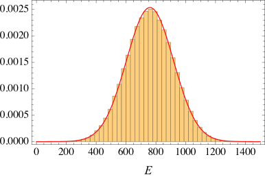
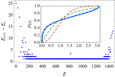
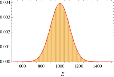
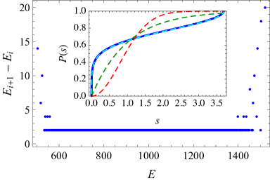
Figure 1: Left: level density histogram (normalized to unity) for the HS chain in a subspace with fixed magnon numbers $N_{1}=N_{2}=13$ ($\mathrm{su}(2)$, top) and $N_{1}=N_{2}=N_{3}=8$ ($\mathrm{su}(3)$, bottom) compared to a Gaussian distribution (continuous red line). Right: differences between consecutive levels of the raw spectrum (main plots) and cumulative spacings distribution of the unfolded spectrum (insets) in the latter configurations. The dashed red, green and light blue curves in the insets are respectively the Wigner (GOE) and Poisson cumulative distributions and the law (7.1). (In all cases, we have used natural units $\hbar=2M=1$.)

We shall next analyze the thermodynamics of a class of LMG models of HS type whose deformation Hamiltonian (2.8) is given by

$$h(x_{1},\dots,x_{m})=\frac{1}{N}\,\sum_{a=1}^{m}(x_{a}-n_{a}N)^{2}\,,$$ (7.2)

where the parameters $n_{a}$ ($1\leqslant a\leqslant m$) are assumed to lie in the interval $(0,1)$ and $n_{1}+\cdots+n_{m}=1$. These parameters thus represent the magnon densities of the ground state in the ferromagnetic case ($\epsilon=1$). The motivation for considering a quadratic deformation Hamiltonian is, first of all, that in the original, isotropic LMG model the external term $H_{1}$ is precisely of this form. More recently, generalized LMG models with a quadratic external term have proved of interest in the context of quantum information theory, since they are some of the few systems for which the bipartite entanglement entropy of the ground state can be computed in closed form [11, 13, 19]. Using the exact formulas (4.8)-(4.12) and (6.6), we have evaluated the partition function of this class of models for a relatively large number of spins, of the order of 100 (resp. $50$) for the $\mathrm{su}(2)$ (resp. $\mathrm{su}(3)$) ferromagnetic LMG-PF models. From the resulting expression, we have computed the free energy $f$, the internal energy $u$, the entropy $s$ and the specific heat $c$ (per spin, in all cases) via the formulas

$$f(T) =-\frac{T}{N}\,\log Z(T)\,,\qquad u(T)=\frac{T^{2}}{N}\,\frac{\partial\log Z(T)}{\partial T}\,,$$ (7.3)

$$s(T) =\frac{\partial}{\partial T}\bigg{(}\frac{T}{N}\log Z(T)\bigg{)}\,,\qquad c(T)=\frac{2T}{N}\,\frac{\partial\log Z(T)}{\partial T}+\frac{T^{2}}{N}\frac{\partial^{2}\log Z(T)}{\partial T^{2}}\,,$$ (7.4)

where we have taken Boltzmann’s constant $k_{\mathrm{B}}=1$. We have first verified that the thermodynamic functions are practically independent of $N$ for $N\lesssim 100$ (in the $\mathrm{su}(2)$ case) and $N\lesssim 50$ (in the $\mathrm{su}(3)$ case). Thus the thermodynamic functions for $N=100$ (in the $\mathrm{su}(2)$ case) and $N=50$ (in the $\mathrm{su}(3)$ case) can be regarded as a reasonable approximation of their $N\to\infty$ counterparts. As an additional check, we have compared the results for the $\mathrm{su}(2)$ PF chain with no deformation Hamiltonian and $N=100$ spins with the exact $N\to\infty$ formulas derived in Ref. [52], finding them in excellent agreement (cf. Fig. 2). In particular, the extensive behavior of the thermodynamic entropy contrasts with the logarithmic growth of the ground-state entanglement entropy of the ferromagnetic “quadratic” gLMG models studied in Ref. [19].

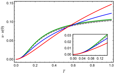
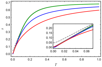
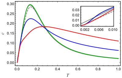
Figure 2: Thermodynamic functions for the $\mathrm{su}(2)$ ferromagnetic LMG-PF model with $h(N_{1},N_{2})=[(N_{1}-n_{1}N)^{2}+(N_{2}-n_{2}N)^{2}]/N$ for $N=100$ spins. The red, blue and green lines correspond respectively to the magnon densities $(n_{1},n_{2})=(1/8,7/8)$, $(1/4,3/4)$ and $(1/2,1/2)$, while the continuous gray line represents the $h=0$, $N=\infty$ exact result. (In all cases, we have used natural units $\hbar=2M=k_{\mathrm{B}}=1$.)

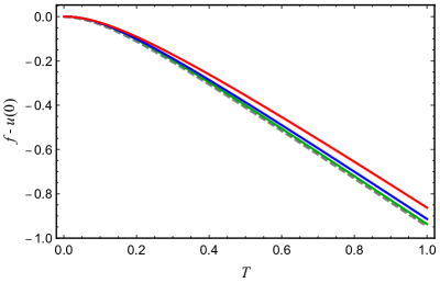
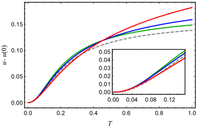
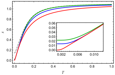
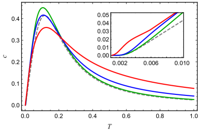
Figure 3: Thermodynamic functions for the $\mathrm{su}(3)$ ferromagnetic LMG-PF model with $h(N_{1},N_{2},N_{3})=\sum_{i=1}^{3}(N_{i}-n_{i}N)^{2}/N$ for $N=50$ spins. The red, blue and green lines correspond respectively to the magnon densities $(n_{1},n_{2},n_{3})=(1/8,1/4,5/8)$, $(1/4,1/4,1/2)$ and $(1/3,1/3,1/3)$. (In all cases, we have used natural units $\hbar=2M=k_{\mathrm{B}}=1$.)

In Figs. 2 and 3 we present the plots of the free and internal energies, the entropy and the specific heat (per spin) respectively of the $\mathrm{su}(2)$ and $\mathrm{su}(3)$ models (2.9)-(7.2) in the PF case. It is apparent from these figures that both the $\mathrm{su}(2)$ and the $\mathrm{su}(3)$ thermodynamic functions qualitatively behave like those of a two-level system, as for instance the one-dimensional Ising model at zero magnetic field or a paramagnetic spin $1/2$ ion [59]. In particular, from Figs. 2 and 3 we see that the specific heat exhibits the Schottky peak characteristic of the latter systems. Finally, it may seem surprising that the entropy per spin does not appear to vanish at $T=0$ in some cases, especially when $h=0$ (see, e.g., Fig. 3). Of course, the explanation for this behavior is that the number of spins $N$ is finite (though large), so that $s(0)=(\log d(m,N))/N$, where $d(m,N)$ is the ground state degeneracy. In the ferromagnetic case under consideration, it follows from Eq. (2.9) that when $h=0$ the ground states are the symmetric states, so that

$$d(m,N)={N+m-1\choose m-1}\simeq\frac{N^{m-1}}{(m-1)!}\,,$$

and thus $s(0)\simeq(m-1)(\log N)/N$ is small but nonzero. On the other hand, when $h$ does not vanish identically the $H_{1}$ term in Eq. (2.9) breaks the ground state degeneracy almost completely (the more so in the less symmetric cases, in which the densities $n_{a}$ are all different), so that $s(0)$ is significantly smaller than its $h=0$ counterpart.

8 Conclusions

We shall finish this paper with a brief summary of its main results. We have introduced a family of generalized $\mathrm{su}(m)$ Lipkin–Meshkov–Glick models whose interacting term is a spin chain of Haldane–Shastry type, which can be equivalently regarded as the deformation of a spin chain of HS type $H_{0}$ by the addition of a term $H_{1}$ in the enveloping algebra of the Cartan subalgebra of $\mathrm{su}(m)$. The Hilbert space of the system is a direct sum of subspaces ${\mathcal{H}}(\mathbf{N})$ with fixed magnon numbers, in which the action of the deformation term is diagonal, so that the model’s partition function decomposes as in Eq. (2.10). By a suitable adaptation of Polychronakos’s freezing trick, we have been able to compute in closed form the partition functions of the restrictions of the spin chain Hamiltonian $H_{0}$ to the subspaces ${\mathcal{H}}(\mathbf{N})$. In view of the previous remarks, this immediately yields the partition function of the associated gLMG model. In particular, when $H_{0}$ is the Hamiltonian of the Polychronakos–Frahm spin chain we have obtained an alternative, simpler expression for the partition function akin to Polychronakos’s formula [42] for the case $H_{1}=0$. This closed-form expression for the partition function of the restriction of $H_{0}$ to the subspaces ${\mathcal{H}}(\mathbf{N})$ has been used in numerical calculations to provide strong evidence that the level density of the latter restriction is Gaussian when the number of spins tends to infinity. In view of the results of Ref. [54], this suggests that there exists a description of the spectrum of $H_{0}\big{|}_{{\mathcal{H}}(\mathbf{N})}$ in terms of motifs, a fact that deserves further investigation. We have also numerically studied the distribution of the spacings of consecutive unfolded levels of $H_{0}\big{|}_{{\mathcal{H}}(\mathbf{N})}$, showing that it follows the same characteristic law previously found for the complete spectrum. As a final application, we have computed the free and internal energies, the entropy and the specific heat per spin of a class of $\mathrm{su}(2)$ and $\mathrm{su}(3)$ gLMG models with quadratic $H_{1}$. We have checked that these functions are virtually independent of the number of spins $N$ when this number is sufficiently large, which indicates that they yield reasonable approximations to their respective thermodynamic limits. Our analysis shows that the thermodynamic functions of these models are qualitatively similar to those of a two-level system, as already observed in Ref. [52] for the $\mathrm{su}(2)$ chains of HS type. In the latter chains, this similarity is ultimately due to the existence of a description of the spectrum in terms of motifs, which leads to simple closed formulas for the thermodynamic functions in terms of the dispersion relation. This again suggests that a description of this type should also exist for the more general models studied in this paper.

References

References

• [1] Lipkin H J, Meshkov N and Glick A J, Validity of many-body approximation methods for a solvable model: (I). Exact solutions and perturbation theory, 1965 Nucl. Phys. 62 188
• [2] Meshkov N, Glick A J and Lipkin H J, Validity of many-body approximation methods for a solvable model: (II). Linearization procedures, 1965 Nucl. Phys. 62 199
• [3] Glick A J, Lipkin H J and Meshkov N, Validity of many-body approximation methods for a solvable model: (III). Diagram summations, 1965 Nucl. Phys. 62 211
• [4] Ring P and Schuck P, The Nuclear Many-Body Problem (Berlin: Springer-Verlag), first edition 1980
• [5] Unanyan R G and Fleischhauer M, Decoherence-free generation of many-particle entanglement by adiabatic ground-state transitions, 2003 Phys. Rev. Lett. 90 133601(4)
• [6] Chen G, Liang J Q and Jia S, Interaction-induced Lipkin–Meshkov–Glick model in a Bose–Einstein condensate inside an optical cavity, 2009 Opt. Express 17 19682
• [7] Ulyanov V V and Zaslavskii O B, New methods in the theory of quantum spin chains, 1992 Phys. Rep. 216 179
• [8] Opanchuk B, Rosales-Zárate L, Teh R Y and Reid M D, Quantifying the mesoscopic quantum coherence of approximate NOON states and spin-squeezed two-mode Bose–Einstein condensates, 2016 Phys. Rev. A 94 062125(14)
• [9] Romera E, Castaños O, Calixto M and Pérez-Bernal F, Delocalization properties at isolated avoided crossings in Lipkin–Meshkov–Glick type Hamiltonian models, 2017 J. Stat. Mech. Theory-E. 2017 P013101(19)
• [10] Popkov V and Salerno M, Logarithmic divergence of the block entanglement entropy for the ferromagnetic Heisenberg model, 2005 Phys. Rev. A 71 012301(4)
• [11] Latorre J I, Orús R, Rico E and Vidal J, Entanglement entropy in the Lipkin–Meshkov–Glick model, 2005 Phys. Rev. A 71 064101(4)
• [12] Barthel T, Dusuel S and Vidal J, Entanglement entropy beyond the free case, 2006 Phys. Rev. Lett. 97 220402(4)
• [13] Orus R, Dusuel S and Vidal J, Equivalence of critical scaling laws for many-body entanglement in the Lipkin–Meshkov–Glick model, 2008 Phys. Rev. Lett. 101 25701(4)
• [14] Wilms J, Vidal J, Verstraete F and Dusuel S, Finite-temperature mutual information in a simple phase transition, 2012 J. Stat. Mech.-Theory E. 2012 P01023(21)
• [15] Vidal G, Latorre J I, Rico E and Kitaev A, Entanglement in quantum critical phenomena, 2003 Phys. Rev. Lett. 90 227902(4)
• [16] Holzhey C, Larsen F and Wilczek F, Geometric and renormalized entropy in conformal field theory, 1994 Nucl. Phys. B 424 443
• [17] Korepin V E, Universality of entropy scaling in one dimensional gapless models, 2004 Phys. Rev. Lett. 92 096402(3)
• [18] Refael G and Moore J E, Entanglement entropy of random quantum critical points in one dimension, 2004 Phys. Rev. Lett. 93 260602(4)
• [19] Carrasco J A, Finkel F, González-López A, Rodríguez M A and Tempesta P, Generalized isotropic Lipkin–Meshkov–Glick models: ground state entanglement and quantum entropies, 2016 J. Stat. Mech. Theory-E. 2016 033114(33)
• [20] Pan F and Draayer J P, Analytical solutions for the LMG model, 1999 Phys. Lett. B 451 1
• [21] Morita H, Ohnishi H, da Providência J and Nishiyama S, Exact solutions for the LMG model Hamiltonian based on the Bethe ansatz, 2006 Nucl. Phys. B 737 337
• [22] Ribeiro P, Vidal J and Mosseri R, Thermodynamical limit of the Lipkin–Meshkov–Glick model, 2007 Phys. Rev. Lett. 99 050402(4)
• [23] Ribeiro P, Vidal J and Mosseri R, Exact spectrum of the Lipkin–Meshkov–Glick model in the thermodynamic limit and finite-size corrections, 2008 Phys. Rev. E 78 021106(13)
• [24] Tsallis C, Possible generalization of Boltzmann–Gibbs statistics, 1988 J. Stat. Phys. 52 479
• [25] Tsallis C, Introduction to Nonextensive Statistical Mechanics: Approaching a Complex World (Berlin: Springer) 2009
• [26] Haldane F D M, Exact Jastrow–Gutzwiller resonating-valence-bond ground state of the spin-$1/2$ antiferromagnetic Heisenberg chain with $1/r^{2}$ exchange, 1988 Phys. Rev. Lett. 60 635
• [27] Shastry B S, Exact solution of an ${S}=1/2$ Heisenberg antiferromagnetic chain with long-ranged interactions, 1988 Phys. Rev. Lett. 60 639
• [28] Haldane F D M, Ha Z N C, Talstra J C, Bernard D and Pasquier V, Yangian symmetry of integrable quantum chains with long-range interactions and a new description of states in conformal field theory, 1992 Phys. Rev. Lett. 69 2021
• [29] Polychronakos A P, Lattice integrable systems of Haldane–Shastry type, 1993 Phys. Rev. Lett. 70 2329
• [30] Frahm H, Spectrum of a spin chain with inverse-square exchange, 1993 J. Phys. A: Math. Gen. 26 L473
• [31] Frahm H and Inozemtsev V I, New family of solvable 1D Heisenberg models, 1994 J. Phys. A: Math. Gen. 27 L801
• [32] Gutzwiller M C, Effect of correlation on the ferromagnetism of transition metals, 1963 Phys. Rev. Lett. 10 159
• [33] Gebhard F and Vollhardt D, Correlation functions for Hubbard-type models: the exact results for the Gutzwiller wave function in one dimension, 1987 Phys. Rev. Lett. 59 1472
• [34] Haldane F D M, “Fractional statistics” in arbitrary dimensions: a generalization of the Pauli principle, 1991 Phys. Rev. Lett. 67 937
• [35] Greiter M and Schuricht D, No attraction between spinons in the Haldane–Shastry model, 2005 Phys. Rev. B 71 224424(4)
• [36] Greiter M, Statistical phases and momentum spacings for one-dimensional anyons, 2009 Phys. Rev. B 79 064409(5)
• [37] Basu-Mallick B, Bondyopadhaya N and Sen D, Low energy properties of the $\mathrm{SU}(m|n)$ supersymmetric Haldane–Shastry spin chain, 2008 Nucl. Phys. B 795 596
• [38] Cirac J I and Sierra G, Infinite matrix product states, conformal field theory, and the Haldane–Shastry model, 2010 Phys. Rev. B 81 104431(4)
• [39] Bargheer T, Beisert N and Loebbert F, Boosting nearest-neighbour to long-range integrable spin chains, 2008 J. Stat. Mech. Theory-E. 2008 L11001(9)
• [40] Bargheer T, Beisert N and Loebbert F, Long-range deformations for integrable spin chains, 2009 J. Phys. A: Math. Theor. 42 285205(58)
• [41] Hung C L, González-Tudela A, Cirac J I and Kimble H J, Quantum spin dynamics with pairwise-tunable, long-range interactions, 2016 Proc. Natl. Acad. Sci. U. S. A. 113 E4946
• [42] Polychronakos A P, Exact spectrum of $\mathrm{SU}(n)$ spin chain with inverse-square exchange, 1994 Nucl. Phys. B 419 553
• [43] Finkel F and González-López A, Global properties of the spectrum of the Haldane–Shastry spin chain, 2005 Phys. Rev. B 72 174411(6)
• [44] Barba J C, Finkel F, González-López A and Rodríguez M A, Inozemtsev’s hyperbolic spin model and its related spin chain, 2010 Nucl. Phys. B 839 499
• [45] Calogero F, Solution of the one-dimensional ${N}$-body problems with quadratic and/or inversely quadratic pair potentials, 1971 J. Math. Phys. 12 419
• [46] Sutherland B, Exact results for a quantum many-body problem in one dimension, 1971 Phys. Rev. A 4 2019
• [47] Sutherland B, Exact results for a quantum many-body problem in one dimension. II, 1972 Phys. Rev. A 5 1372
• [48] Inozemtsev V I, Exactly solvable model of interacting electrons confined by the Morse potential, 1996 Phys. Scr. 53 516
• [49] Berry M V and Tabor M, Level clustering in the regular spectrum, 1977 Proc. R. Soc. London Ser. A 356 375
• [50] Bohigas O, Giannoni M J and Schmit C, Characterization of chaotic quantum spectra and universality of level fluctuation laws, 1984 Phys. Rev. Lett. 52 1
• [51] Barba J C, Finkel F, González-López A and Rodríguez M A, The Berry–Tabor conjecture for spin chains of Haldane–Shastry type, 2008 Europhys. Lett. 83 27005(6)
• [52] Enciso A, Finkel F and González-López A, Thermodynamics of spin chains of Haldane–Shastry type and one-dimensional vertex models, 2012 Ann. Phys.-New York 327 2627
• [53] Enciso A, Finkel F and González-López A, Spin chains of Haldane–Shastry type and a generalized central limit theorem, 2009 Phys. Rev. E 79 060105(4)
• [54] Enciso A, Finkel F and González-López A, Level density of spin chains of Haldane–Shastry type, 2010 Phys. Rev. E 82 051117(6)
• [55] Basu-Mallick B, Bondyopadhaya N and Hikami K, One-dimensional vertex models associated with a class of Yangian invariant Haldane–Shastry like spin chains, 2010 SIGMA 6 091(13)
• [56] Haake F, Quantum Signatures of Chaos (Berlin: Springer-Verlag), second edition 2001
• [57] Barba J C, Finkel F, González-López A and Rodríguez M A, Polychronakos–Frahm spin chain of $BC_{N}$ type and the Berry–Tabor conjecture, 2008 Phys. Rev. B 77 214422(10)
• [58] Barba J C, Finkel F, González-López A and Rodríguez M A, An exactly solvable supersymmetric spin chain of $BC_{N}$ type, 2009 Nucl. Phys. B 806 684
• [59] Mussardo G, Statistical Field Theory: an Introduction to Exactly Solved Models in Statistical Physics (Oxford: Oxford University Press) 2010