The optimal particle-mesh interpolation basis

Abstract

The fast Ewald methods are widely used to compute the point-charge electrostatic interactions in molecular simulations. The key step that introduces errors in the computation is the particle-mesh interpolation. In this work, the optimal interpolation basis is derived by minimizing the estimated error of the fast Ewald method. The basis can be either general or model specific, depending on whether or not the charge correlation has been taken into account. By using the TIP3P water as an example system, we demonstrate that the general optimal basis is always more accurate than the B-spline basis in the investigated parameter range, while the computational cost is at most 5% more expensive. In some cases, the optimal basis is found to be two orders of magnitude more accurate. The model specific optimal basis further improves the accuracy of the general optimal basis, but requires more computational effort in the optimization, and may not be transferable to systems with different charge correlations. Therefore, the choice between the general and model specific optimal bases is a trade-off between the generality and the accuracy.

I Introduction

The computation of the electrostatic interaction is an important and non-trivial task in molecular simulations. The difficulty lies in the slow decay of the Coulomb interaction with respect to the particle distance, thus the cut-off method that ignores the particle interactions beyond a certain range usually leads to unphysical artifacts vanderSpoel2006origin . This problem is solved by the Ewald summation ewald1921die , which splits the electrostatic interaction into a short-ranged particle-particle interaction that is computed by the cut-off method and an interaction of smeared charges that is computed by solving the Poisson equation in the reciprocal space. The optimal computational expense of the Ewald summation grows in proportion to the three-halves power of the number of particles, and is unaffordable for systems that are larger than several hundreds of particles pollock1996comments .

Instead of the Ewald summation, the fast Ewald methods are widely used nowadays and implemented in molecular simulation packages pronk2013gromacs ; phillips2005scalable ; plimpton1995fast . Some examples are the smooth particle mesh Ewald (SPME) method darden1993pme ; essmann1995spm , the particle-particle particle-mesh (PPPM) method hockney1988computer ; deserno1998mue1 and the nonequispaced fast Fourier transform based method hedman2006ewald ; pippig2013pfft . These methods reduce the computational expense to $\mathcal{O}(N\log N)$ ($N$ being the number of particles) by accelerating the solution of the Poisson equation with the fast Fourier transform (FFT). Although the fast Ewald methods are substantially faster than the Ewald summation, the accuracy is inferior. The only step that introduces errors is the particle-mesh interpolation, which interpolates the particle charges on a uniform mesh, and the solution of the Poisson equation represented on the mesh back to the particles. Therefore, the quality of the interpolation basis plays an important role in the accuracy of the fast Ewald methods deserno1998mue2 ; wang2010optimizing ; ballenegger2012convert ; wang2012numerical .

All the mentioned fast Ewald methods use the cardinal B-spline basis for the particle-mesh interpolation, which was proved to be superior to the Lagrangian interpolation basis deserno1998mue1 . Very recently, Nestler nestler2016parameter and Gao et. al. gao2017kaiser showed that the Bessel and Kaiser-Bessel bases are more accurate than the B-spline basis in certain ranges of the working parameter space, which is spanned by the splitting parameter (how the two parts of the Ewald summation are split), the mesh spacing and the truncation radius of the interpolation basis. These observations indicate that the B-spline basis that is the “golden standard” in the particle-mesh interpolation can be improved, at least, in part of the parameter space.

In this work, the optimal particle-mesh interpolation basis in the sense of minimizing the estimated error of the fast Ewald method is proposed. In our approach, the optimal basis is discretized by the cubic Hermite splines, and the values and derivatives of the basis at the discretization nodes are adjusted by solving an unconstrained optimization problem. We prove that, as long as the system size is large enough, the optimal interpolation basis is system independent, and is determined by a characteristic number defined by the product of the splitting parameter and the mesh spacing. We numerically investigate the accuracy of the optimal interpolation basis in a TIP3P water system, and demonstrate that the optimal basis always outperforms the B-spline and the Kaiser-Bessel bases in the investigated parameter range. In some cases, the optimal basis is more than two orders of magnitude more accurate than the B-spline and the Kaiser-Bessel bases. We also show that the time-to-solution of using the optimal basis is marginally longer than the B-spline basis, and is no more than the Kaiser-Bessel basis. We report that the accuracy of the optimal basis is further improved by taking into account the charge correlations during the basis optimization. However, the derived optimal basis is model specific, and cannot be transferred to the simulation with the same product of the splitting parameter and the mesh spacing. This implies that when simulating systems with different charge correlations, the basis should be re-optimized. Therefore, whether or not to consider the charge correlation in the basis optimization is a trade-off between the generality and the accuracy.

The manuscript is organized as follows: In Sec. II, the fast Ewald method is introduced briefly. The optimal interpolation basis is proposed in Sec. III, and the generality of the optimal basis is discussed in Sec. IV. In Sec. V, the accuracy of the optimal basis is investigated in the TIP3P water system as an example, and the advantage over the B-spline and the Kaiser-Bessel bases is demonstrated. In Sec. VI, we show that the accuracy of the optimal basis is further improved, at the cost of generality, by taking into account the charge correlation in the system. The work is concluded in Sec. VII.

II The fast Ewald methods

We consider $N$ point charges that are denoted by $\{q_{1},\cdots,q_{N}\}$ in a unit cell with periodic boundary condition. The positions of the charges are denoted by $\{\textbf{{r}}_{1},\cdots,\textbf{{r}}_{N}\}$, respectively. The Coulomb interaction of the unit cell is given by

$$E=\frac{1}{2}\sum_{\textbf{{n}}}^{\ast}\sum_{i,j=1}^{N}\frac{q_{i}q_{j}}{|\textbf{{r}}_{ij}+\textbf{{n}}|},$$ (1)

where $\textbf{{r}}_{ij}=\textbf{{r}}_{i}-\textbf{{r}}_{j}$, and $\textbf{{r}}_{ij}+\textbf{{n}}$ is the distance between charge $i$ and all periodic images of charge $j$, because we have $\textbf{{n}}=n_{1}\textbf{{a}}_{1}+n_{2}\textbf{{a}}_{2}+n_{3}\textbf{{a}}_{3}$ with $(n_{1},n_{2},n_{3})\in\mathbb{Z}^{3}$ and $(\textbf{{a}}_{1},\textbf{{a}}_{2},\textbf{{a}}_{3})$ being the unit cell vectors. The “$\ast$” over the outer summation means that when $\textbf{{n}}=0$, the $i=j$ terms should be skipped in the inner summation. The prefactor $1/(4\pi\epsilon_{0})$ is omitted for simplicity. The origin of the prefactor $1/2$ is explained in Ref. ballenegger2009simulations . The Ewald summation splits the Coulomb interaction into the direct, reciprocal and correction contributions, i.e. $E=E_{\mathrm{dir}}+E_{\mathrm{rec}}+E_{\mathrm{correction}}$ with

$$E_{\mathrm{dir}}=\frac{1}{2}\sum^{\ast}_{\textbf{{n}}}\sum_{i,j=1}^{N}\frac{q_{i}q_{j}\mathrm{erfc}(\beta|\textbf{{r}}_{ij}+\textbf{{n}}|)}{|\textbf{{r}}_{ij}+\textbf{{n}}|},$$ (2)

$$E_{\mathrm{rec}}=\frac{1}{2\pi V}\sum_{\textbf{{m}}\neq 0}\frac{\exp(-\pi^{2}\textbf{{m}}^{2}/\beta^{2})}{\textbf{{m}}^{2}}S(\textbf{{m}})S(-\textbf{{m}}),$$ (3)

$$E_{\mathrm{correction}}=-\frac{\beta}{\sqrt{\pi}}\sum_{i=1}^{N}q_{i}^{2}.$$ (4)

We omit the surface energy term because the spherical summation order and the metallic boundary condition are assumed to the system ballenegger2009simulations ; de1980simulation ; de1980simulation2 . In the Ewald summation, $\beta>0$ is the splitting parameter that controls the convergence speed of the direct and the reciprocal parts. In the reciprocal energy (3), $\textbf{{m}}=m_{1}\textbf{{a}}_{1}^{\ast}+m_{2}\textbf{{a}}_{2}^{\ast}+m_{3}\textbf{{a}}_{3}^{\ast}$ with $(m_{1},m_{2},m_{3})\in\mathbb{Z}^{3}$ and $(\textbf{{a}}^{\ast}_{1},\textbf{{a}}^{\ast}_{2},\textbf{{a}}^{\ast}_{3})$ being the reciprocal cell vectors defined by $\textbf{{a}}_{\alpha}\cdot\textbf{{a}}_{\gamma}^{\ast}=\delta_{\alpha\gamma}$, where $\alpha,\gamma=1,2,3$. $V=(\textbf{{a}}_{1}\times\textbf{{a}}_{2})\cdot\textbf{{a}}_{3}$ is the volume of the unit cell. $S(\textbf{{m}})=\sum_{j=1}^{N}q_{j}e^{2\pi\mathrm{i}\textbf{{m}}\cdot\textbf{{r}}_{j}}$ is the structure factor, and the notation “$\mathrm{i}$” at the exponent should be understood as the imaginary unit (not a charge index). The magnitude of the structure factor is upper bounded by $\sum_{j}|q_{j}|$.

In the direct energy part (2), the complementary error function, i.e. $\mathrm{erfc}$, converges exponentially fast to zero with increasing charge distance $|\textbf{{r}}_{ij}+\textbf{{n}}|$, therefore, it can be cut off and the direct energy is computed at the cost of $\mathcal{O}(N)$ by using the standard cell division and neighbor list algorithms frenkel2001understanding . The summand of the reciprocal energy (3) decays exponentially fast as $|\textbf{{m}}|$ increases, therefore, the infinite summation can be approximated by a finite summation, where $m_{\alpha}$ ranges from $-K_{\alpha}/2$ to $K_{\alpha}/2-1$ with $K_{\alpha}$ being the number of terms summed on direction $\alpha$. A naive choice of $K_{\alpha}$ that preserves the accuracy satisfies $K_{1}K_{2}K_{3}\propto N$, thus the computational complexity of the reciprocal energy is $\mathcal{O}(N^{2})$.

The fast Ewald methods interpolate the point charges on a $K_{1}\times K_{2}\times K_{3}$ uniform mesh, then accelerate the computation of the structure factor, which is a discretized Fourier transform of the charge distribution, by the fast Fourier transform (FFT). Taking the SPME method as an example, the interpolation of the single particle charge contribution to the mesh (on direction $\alpha$) reads wang2016multiple

$$qe^{2\pi\mathrm{i}m_{\alpha}u_{\alpha}/K_{\alpha}}\approx\frac{1}{K_{\alpha}\hat{\varphi}(m_{\alpha})}\sum_{l\in I_{K}}q\,\varphi(u_{\alpha}-l)e^{2\pi\mathrm{i}m_{\alpha}l/K_{\alpha}},$$ (5)

where $u$ is the scaled coordinate that is defined by $u_{\alpha}=K_{\alpha}r_{\alpha}$ with $r_{\alpha}=\textbf{{a}}^{\ast}_{\alpha}\cdot\textbf{{r}}$. $I_{K}=\{l\in\mathbb{Z}:-K/2\leq l<K/2\}$. $\varphi$ is the interpolation basis that is usually assumed to be truncated with radius $C$, which means the value of $\varphi$ out of the range $[-C,C]$ is assume to be 0. The Fourier transform of $\varphi$ on $I_{K}$ is denoted by $\hat{\varphi}$. By using the approximation (5), the reciprocal energy is proved to be essmann1995spm

$$E_{\mathrm{rec}}\approx\sum_{l_{1},l_{2},l_{3}}Q(l_{1},l_{2},l_{3})[\,Q\ast(FB^{2})^{\vee}](l_{1},l_{2},l_{3}),$$ (6)

where “$\ast$” denotes the convolution, “$\vee$” denotes the inverse discrete Fourier transform, and

$$F(\textbf{{m}})=\frac{1}{2\pi V}\times\begin{dcases}\frac{\exp(-\pi^{2}\textbf{{m}}^{2}/\beta^{2})}{\textbf{{m}}^{2}}&|\textbf{{m}}|\neq 0,\\ \>0&|\textbf{{m}}|=0,\end{dcases}$$ (7)

$$B(\textbf{{m}})=\prod_{\alpha}\frac{1}{\hat{\varphi}(m_{\alpha})},$$ (8)

$$P_{\textbf{{r}}}(l_{1},l_{2},l_{3})=\prod_{\alpha}\varphi(u_{\alpha}-l_{\alpha}),$$ (9)

$$Q(l_{1},l_{2},l_{3})=\sum_{j}q_{j}P_{\textbf{{r}}_{j}}(l_{1},l_{2},l_{3}).$$ (10)

$Q(l_{1},l_{2},l_{3})$ is the interpolated charge distribution on the mesh. The interpolation of single particle to mesh, viz. the computation of $P_{\textbf{{r}}}(l_{1},l_{2},l_{3})$, can be accomplished in $\mathcal{O}(1)$ operations due to the compact support of the interpolation basis $\varphi$, thus the computational cost of $Q=\sum_{j}q_{j}P_{\textbf{{r}}_{j}}$ is $\mathcal{O}(N)$. By using the identity $Q\ast(FB^{2})^{\vee}=[\,\hat{Q}\times(FB^{2})\,]^{\vee}$, the computation of the convolution in Eq. (6) is converted to a forward discrete Fourier transform of $Q$, a multiplication between $\hat{Q}$ and $FB^{2}$, and then a backward transform of $\hat{Q}\times(FB^{2})$. The computational cost of the multiplication is $\mathcal{O}(N)$ and that of the fast Fourier transforms is $\mathcal{O}(N\log N)$, thus the total computational cost of the reciprocal energy (6) is $\mathcal{O}(N\log N)$.

The reciprocal force of a charged particle can be computed in two ways. The first way, known as ik-differentiation, takes negative gradient of the reciprocal energy (3) with respect to particle coordinate r, then approximates the force by the particle-mesh interpolation. It leads to darden1993pme

$$\textbf{{F}}^{\mathrm{ik}}_{\mathrm{rec},i}\approx\ q_{i}\sum_{l_{1},l_{2},l_{3}}P_{\textbf{{r}}_{i}}(l_{1},l_{2},l_{3})[\,Q\ast(\textbf{{G}}B^{2})^{\vee}](l_{1},l_{2},l_{3}),$$ (11)

where

$$\textbf{{G}}(\textbf{{m}})=-4\pi\mathrm{i}\textbf{{m}}F(\textbf{{m}}).$$ (12)

The second way, known as analytical differentiation, takes negative gradient of the approximated reciprocal energy (6), and yields essmann1995spm

$$\textbf{{F}}^{\mathrm{ad}}_{\mathrm{rec},i}\approx\ q_{i}\sum_{l_{1},l_{2},l_{3}}-2\nabla_{\textbf{{r}}_{i}}P_{\textbf{{r}}_{i}}(l_{1},l_{2},l_{3})[\,Q\ast(FB^{2})^{\vee}](l_{1},l_{2},l_{3}).$$ (13)

In the energy approximation (6) and force approximations (11) and (13), the only step that introduces errors is the particle-mesh interpolation (5), thus the interpolation basis plays a crucial role in the accuracy of the fast Ewald methods. In the original work of the SPME and PPPM methods essmann1995spm ; hockney1988computer , the B-spline basis was proposed for the interpolation. An $n$-th order B-spline basis is defined in a recursive way:

$$\varphi_{n}(x)=K\varphi_{n-1}\ast\varphi_{1}(x),\quad\varphi_{1}(x)=\chi_{[-1/2,1/2]}(x),$$ (14)

where $\chi_{[-1/2,1/2]}(x)$ is the characteristic function of interval $[-1/2,1/2]$. The order $n$ B-spline basis has a compact support of $[-n/2,n/2]$, and is $(n-2)$-th order differentiable. The basis truncation is usually taken as $C=n/2$. The Kaiser-Bessel basis of truncation $C$ is defined by

$$\varphi(x)=\frac{\sinh(\pi H\sqrt{C^{2}-x^{2}})}{\pi\sqrt{C^{2}-x^{2}}},$$ (15)

where $H$ is the shape parameter, which can be determined by optimizing against the reciprocal force error gao2017kaiser .

III The optimal interpolation basis

The quality of the interpolation basis can be investigated by evaluating the error introduced in the computation. In the context of molecular dynamics (MD) simulations, the error is usually defined by the root mean square (RMS) error of the reciprocal force computation, i.e.

$$\mathcal{E}=\sqrt{\langle|\Delta\textbf{{F}}_{\mathrm{rec}}|^{2}\rangle},\quad\Delta\textbf{{F}}_{\mathrm{rec}}=\textbf{{F}}_{\mathrm{rec}}-\textbf{{F}}_{\mathrm{rec}}^{\ast},$$ (16)

where $\langle\cdot\rangle$ denotes the ensemble average, and $\textbf{{F}}_{\mathrm{rec}}$ and $\textbf{{F}}_{\mathrm{rec}}^{\ast}$ denote the computed and exact reciprocal forces, respectively. It has been shown that the RMS reciprocal error is composed of the homogeneity, the inhomogeneity and the correlation parts wang2012numerical

$$|\mathcal{E}|^{2}=|\mathcal{E}_{\mathrm{homo}}|^{2}+|\mathcal{E}_{\mathrm{inhomo}}|^{2}+\mathcal{E}_{\mathrm{corr}}.$$ (17)

The homogeneity error $\mathcal{E}_{\mathrm{homo}}$ stems from the fluctuation of the error force $\Delta\textbf{{F}}_{\mathrm{rec}}$. The inhomogeneity error $\mathcal{E}_{\mathrm{inhomo}}$ originates from the inhomogeneous charge distribution, and has been shown to vanish when the system is locally neutral, which is the case in most realistic systems. The correlation error $\mathcal{E}_{\mathrm{corr}}$ contributes when the positions of the charges are correlated. For example, the partial charges in a classical point-charge water system is correlated via the covalent bonds, the hydrogen bonds and the van der Waals interactions.

An error estimate is an analytical expression of the RMS reciprocal force error in terms of the working parameters including the splitting parameter, the mesh spacing and the basis truncation. If the system is locally neutral and the positions of the charges are uncorrelated, the inhomogeneity and the correlation errors vanish, and the errors of the ik- and analytical differentiation force schemes are estimated by wang2016multiple

$$|\mathcal{E}^{\mathrm{ik}}|^{2} =|\mathcal{E}^{\mathrm{ik}}_{\mathrm{homo}}|^{2}\approx 2q^{2}Q^{2}\sum_{\textbf{{m}}}\sum_{\alpha,l\neq 0}\boldsymbol{\mathcal{G}}^{2}_{\alpha,l}(\textbf{{m}}),$$ (18)

$$|\mathcal{E}^{\mathrm{ad}}|^{2} =|\mathcal{E}^{\mathrm{ad}}_{\mathrm{homo}}|^{2}\approx q^{2}Q^{2}\sum_{\textbf{{m}}}\sum_{\alpha,l\neq 0}\boldsymbol{\mathcal{G}}^{2}_{\alpha,l}(\textbf{{m}})+q^{2}Q^{2}\sum_{\textbf{{m}}}\sum_{\alpha,l\neq 0}(\boldsymbol{\mathcal{G}}_{\alpha,l}+\boldsymbol{\mathcal{F}}_{\alpha,l})^{2}(\textbf{{m}}),$$ (19)

where $Q^{2}=\sum_{i}q_{i}^{2}$, $q^{2}=Q^{2}/N$, and we have the short-hand notations

$$\boldsymbol{\mathcal{G}}_{\alpha,l}(\textbf{{m}}) =\textbf{{G}}(\textbf{{m}})Z_{\alpha,l}(\textbf{{m}}),$$ (20)

$$\boldsymbol{\mathcal{F}}_{\alpha,l}(\textbf{{m}}) =-4\pi\mathrm{i}lK_{\alpha}\textbf{{a}}_{\alpha}^{\ast}F(\textbf{{m}})Z_{\alpha,l}(\textbf{{m}}),$$ (21)

$$Z_{\alpha,l}(\textbf{{m}}) ={\hat{\varphi}(m_{\alpha}+lK_{\alpha})}/{\hat{\varphi}(m_{\alpha})}.$$ (22)

The RMS reciprocal error estimates (18) and (19) clearly depend on the interpolation basis. The optimal interpolation basis in terms of minimal numerical error is determined by solving the unconstrained optimization problem

$$\min_{\varphi}\mathcal{E}[\varphi],$$ (23)

where $\mathcal{E}$ can be estimated by either (18) or (19) for ik- or analytical differentiation, respectively. It is reasonable to assume that the interpolation basis is an even function on $[-C,C]$, thus only the value of $\varphi$ in range $[0,C]$ should be determined. We uniformly discretize the range $[0,C]$ by $M$ nodes that are denoted by $x_{i}=i\Delta x$ with $\Delta x=C/M$, and use the following ansatz to construct $\varphi$

$$\varphi(x)=\eta_{0}(x)+\sum_{i=1}^{M-1}\lambda_{i}\eta_{i}(x)+\sum_{i=1}^{M-1}\nu_{i}\theta_{i}(x),$$ (24)

where

$$\eta_{0}(x) =H_{00}(\frac{x-x_{i}}{\Delta x}),$$ (25)

$$\eta_{i}(x) =H_{01}(\frac{x-x_{i-1}}{\Delta x})+H_{00}(\frac{x-x_{i}}{\Delta x}),$$ (26)

$$\theta_{i}(x) =\Delta xH_{11}(\frac{x-x_{i-1}}{\Delta x})+\Delta xH_{10}(\frac{x-x_{i}}{\Delta x}).$$ (27)

$H_{00}$, $H_{01}$, $H_{10}$ and $H_{11}$ are cubic Hermite splines (third order piecewise polynomials, details provided in Appendix A). By this construction, the interpolation basis $\varphi(x)$ is first order differentiable and is normalized by $\varphi(0)=1$. The basis smoothly vanishes at the truncation $x=C$, viz. $\varphi(C)=0$ and $\varphi^{\prime}(C)=0$. The prefactors $\{\lambda_{i}\}$ and $\{\nu_{i}\}$ are the values and derivatives of the basis at the discretization nodes, because it can be proved that $\lambda_{i}=\varphi(x_{i})$ and $\nu_{i}=\varphi^{\prime}(x_{i})$ (see Appendix A for details). By inserting Eq. (24) into error estimates (18) and (19), the functionals of the interpolation basis $\varphi$ are converted into functions of $\{\lambda_{i}\}$ and $\{\nu_{i}\}$. Thus the optimization problem (23) is discretized as

$$\min_{\{\lambda_{i}\},\{\nu_{i}\}}\mathcal{E}(\{\lambda_{i}\},\{\nu_{i}\}).$$ (28)

Since the error estimates (30) and (31) are positive definite and are provided in squared form, it is more convenient to solve the equivalent optimization problem

$$\min_{\{\lambda_{i}\},\{\nu_{i}\}}|\mathcal{E}(\{\lambda_{i}\},\{\nu_{i}\})|^{2}.$$ (29)

This is a classic unconstrained optimization problem, which can be solved by well established algorithms such as conjugate gradient method or Broyden-Fletcher-Goldfarb-Shanno (known as BFGS) method fletcher1987practical . Our code uses the implementation of the BFGS method from Dlib king2009dlib .

IV The generality of the optimal basis

The error estimates (18) and (19) depend on the system, thus the optimization problem (23) should be solved for each specific system to obtain the optimal basis. In this section, we demonstrate that there exists a general optimal basis that minimizes the estimated error in systems with different amounts of charge per particle, different number of charges and different system sizes, as long as the system is large enough.

To begin with, it is more convenient to investigate the properties of the error estimates if the summations in (18) and (19) are converted to integrations, which are referred to as the continuous forms of the error estimates. To simplify the discussion, we assume that the simulation region is cuboid. We denote the mesh spacing on direction $\alpha$ by $h_{\alpha}=L_{\alpha}/K_{\alpha}$, where $L_{\alpha}=|\textbf{{a}}_{\alpha}|$, and further assume that the mesh spacings are roughly the same on all directions, i.e. $h\approx h_{1}\approx h_{2}\approx h_{3}$. The continuous form of the error estimate (18) is (see Appendix B for details)

$$|\mathcal{E}^{\mathrm{ik}}_{\mathrm{homo}}|^{2}\approx\frac{4q^{4}\rho\beta}{(\beta h)^{3}}\int_{I^{3}}g^{2}\Big{(}{|\boldsymbol{\mu}|}/{(\beta h)}\Big{)}\sum_{\alpha,l\neq 0}2z^{2}(\mu_{\alpha},l)\>d\boldsymbol{\mu},$$ (30)

where $\rho=N/V$ is the number density of charged particles in the system. The integration region is defined by $I^{3}=[-1/2,1/2]\times[-1/2,1/2]\times[-1/2,1/2]$. We denote $\boldsymbol{\mu}=(\mu_{1},\mu_{2},\mu_{3})$, $g(m)={e^{-\pi^{2}m^{2}}}/{m}$, and $z(\mu_{\alpha},l)={\tilde{\varphi}(\mu_{\alpha}+l)}/{\tilde{\varphi}(\mu_{\alpha})}$ with $\tilde{\varphi}(\mu)=\int_{[-C,C]}\varphi(x)\ e^{-2\pi\mathrm{i}\mu x}dx$. The continuous form of the error estimate (19) is

$$|\mathcal{E}^{\mathrm{ad}}_{\mathrm{homo}}|^{2}\approx\frac{4q^{4}\rho\beta}{(\beta h)^{3}}\int_{I^{3}}g^{2}\Big{(}{|\boldsymbol{\mu}|}/{(\beta h)}\Big{)}\sum_{\alpha,l\neq 0}\Bigg{[}\Big{(}1+\frac{|\boldsymbol{\mu}+l\textbf{{e}}_{\alpha}|^{2}}{|\boldsymbol{\mu}|^{2}}\Big{)}z^{2}(\mu_{\alpha},l)\Bigg{]}\>d\boldsymbol{\mu}.$$ (31)

It is noted that the continuous forms (30) and (31) do not depend on the system size. As shown in Appendix B, the standard error estimates (18) and (19) are discretizations of the continuous error estimates (30) and (31), respectively, with $K_{\alpha}$ being the number of discretization points on direction $\alpha$. The difference between the standard and the continuous error estimates is the error of the discretization, which vanishes as $K_{\alpha}$ goes to infinity. It is noted that when taking the limit, the mesh spacing $h$ is fixed, thus the limit implies that the system size $L_{\alpha}=hK_{\alpha}$ goes to infinity. Therefore, when the system is large enough, the optimal bases that minimize the standard error estimates converge to the bases that minimize the corresponding continuous error estimates, which are system-size independent.

Before further investigating the properties of the optimal basis, we will firstly show when a standard error estimate converges to its continuous form. The standard error estimate is close to the continuous form only when the variation of the integrand is resolved by enough discretization points. In order to resolve the variation of $g^{2}({|\boldsymbol{\mu}|}/{(\beta h)})$, the characteristic size $\beta h/(\sqrt{2}\,\pi)$ should be discretized by enough points. If two discretization points are required for the size $\beta h/(\sqrt{2}\,\pi)$, then $K_{\alpha}\geq 2\sqrt{2}\pi/(\beta h)$, or equivalently $L_{\alpha}=hK_{\alpha}\geq 2\sqrt{2}\pi/\beta$. This indicates that converged system size is inversely proportional to the splitting parameter $\beta$. Taking the B-spline basis for instance, the convergence of the error estimate (18) with respect to the system size is numerically investigated in Fig. 1. When $\beta=1.0\ \textrm{nm}^{-1}$, the system size should be larger than $4.5$ nm to have a converged error estimate. When $\beta$ increases to $1.5\ \textrm{nm}^{-1}$, the minimal system size is $3.0$ nm. The minimal system size reduces to 2.3 nm when $\beta=2.0\ \textrm{nm}^{-1}$. Although the minimal size is lower than the rough estimate $2\sqrt{2}\pi/\beta\approx 8.9/\beta$, the inversely proportional relation between the minimal size and the splitting parameter is confirmed. It is also observed that the minimal system size does not depend on the basis truncation.

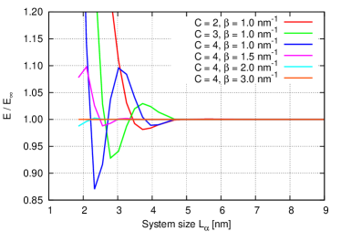
Figure 1: The convergence of the error estimate (18) to the continuous form (30). It is noted that the continuous form is system-size independent. The interpolation basis is B-spline. The mesh spacing is $h=0.117$ nm. We assume that $L_{\alpha}$ is the same on all directions, and plot the ratio between the error estimated in a system of size $L_{\alpha}$ and the error estimated in a fully converged system of size $14.9$ nm. The lines with different colors denote different parameter choices as listed in the legend.

In this work, if not stated otherwise, we always assume that the system size is large enough, so the error estimates (18) and (19) converge to the continuous forms (30) and (31), respectively, and the optimal bases are also converged. The properties of an optimal basis can be analyzed by investigating the corresponding continuous error estimate. For a given basis truncation $C$, the optimal basis has the following properties

1. The optimal basis is independent of the amount of charge per particle.

2. The optimal basis is independent of the number of charged particles.

3. The optimal basis is independent of the size of the system.

4. The optimal basis is completely determined by the characteristic number $\beta h$.

Property 1 holds because the average amount of charge $q^{2}=\sum_{i}q_{i}^{2}/N$ is a prefactor of the error estimates (30) and (31). Property 3 holds because the error estimates are independent of the system size. Property 2 holds because the number density $\rho$ is a prefactor of the error estimates, and because Property 3 holds. When the truncation $C$ is fixed, the integrands of (30) and (31) only depend on the number $\beta h$ via function $g^{2}({|\boldsymbol{\mu}|}/{(\beta h)})$, so the optimal basis is completely determined by this number. Therefore, the optimal interpolation basis is system independent in the sense that it applies to systems with different amounts of charge per particle, different numbers of charges and different system sizes.

Due to the universality of the optimal interpolation basis, the solutions to the optimization problem (29) are stored in a database. The number of discretization nodes of the basis is set to $M=40\,C$. The mesh spacing is set to $0.117$ nm. The number of mesh points is $K_{\alpha}=64$ to ensure the convergence of error estimates. The basis is optimized for a $\beta$ sequence starting from $1.0\ \textrm{nm}^{-1}$, increasing with a step of $0.2\ \textrm{nm}^{-1}$, and ending at $3.4\ \textrm{nm}^{-1}$, and from $4.0\ \textrm{nm}^{-1}$, increasing with a step of $1.0\ \textrm{nm}^{-1}$, and ending at $7.0\ \textrm{nm}^{-1}$. This provides the optimal bases for a $\beta h$ sequence that ranges from 0.117 to 0.818. The optimal basis of the $\beta h$ that is not in the sequence is constructed by linear interpolation of neighboring optimal basis in the sequence.

V The numerical results

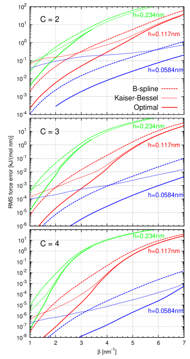
Figure 2: The RMS reciprocal force error of the B-spline (dashed lines), the Kaiser-Bessel (dotted lines) and the optimal (solid lines) bases plotted against the splitting parameter $\beta$ in the TIP3P water system. The force scheme is the ik-differentiation. From top to bottom, the three plots present the basis truncations of $C=2$, 3 and 4, respectively. The green, red and blue lines present the mesh spacings of 0.234, 0.117 and 0.0584 nm, respectively.

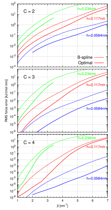
Figure 3: The RMS reciprocal force error of the B-spline (dashed lines) and the optimal (solid lines) bases plotted against the splitting parameter $\beta$ in the TIP3P water system. The force scheme is the analytical differentiation. From top to bottom, the three plots present the basis truncations of $C=2$, 3 and 4, respectively. The green, red and blue lines present the mesh spacings of 0.234, 0.117 and 0.0584 nm, respectively.

In this section, we investigate the RMS reciprocal force error of the B-spline, the Kaiser-Bessel and the optimal bases in a TIP3P jorgensen1983comparison water system that has 13824 molecules. Each water molecule is modeled by three point charges connected by covalent bonds. The oxygen atom has a partial charge of $-0.834\,e$ while the hydrogen atom has a partial charge of $0.417\,e$. The O-H bond length is constrained to 0.09572 nm and the H-O-H angle is constrained to $104.52^{\circ}$. The simulation region is of size $7.48\,\textrm{nm}\times 7.48\,\textrm{nm}\times 7.48\,\textrm{nm}$, and is subjected to the periodic boundary condition. The water configuration is taken from an equilibrated NPT simulation gao2016sampling . The computed reciprocal force is compared with a well converged Ewald summation, and the RMS reciprocal force error is computed by definition (16).

In Fig. 2, we report the RMS force errors of the B-spline (dashed line), the Kaiser-Bessel (dotted line) and the optimal (solid line) bases using the ik-differentiation force scheme. In Fig. 3, we report the RMS force errors of the B-spline (dashed line) and the optimal (solid line) bases using the analytical differentiation force scheme. In both figures, the error is plotted against the splitting parameter $\beta$. The three plots, from top to bottom, present the results of basis truncations $C=2$, 3 and 4, respectively. In each plot, the green, red and blue lines present the errors of the mesh spacings $h=0.234$, 0.117 and 0.0584 nm, respectively. In all cases, the optimal basis is more accurate than the B-spline and the Kaiser-Bessel bases. In some cases, the optimal basis achieves two orders of magnitude higher accuracy, for example, the ik-differentiation with $C=4$, $\beta=3.0~{}\textrm{nm}^{-1}$ and $h=0.0584$ nm. The advantage of the optimal basis is observed to be more significant for smaller splitting parameters, and smaller mesh spacings. Taking the ik-differentiation with $C=3$ and $h=0.117$ nm for example, the optimal basis is 2.1, 9.7 and 35 times as accurate as the B-spline basis and is 1.0, 1.9, and 34 times as accurate as the Kaiser-Bessel basis at $\beta=6.0$, 4.0 and $2.0~{}\textrm{nm}^{-1}$, respectively. Taking $C=3$ and $\beta=3.0~{}\textrm{nm}^{-1}$ for example, the optimal basis is 1.8, 24 and 35 times as accurate as the B-spline basis, and is 1.0, 6.9 and 165 times as accurate as the Kaiser-Bessel basis at mesh spacings $h=0.234$, 0.117 and 0.0584 nm, respectively.

It is noted that the basis that was optimized at $h=0.117$ nm is used for the simulations at $h=0.234$ nm and $h=0.0584$ nm if the products of $\beta h$ are the same. For example, the basis optimized for $\{h=0.117\,\textrm{nm},\ \beta=2.0\,\textrm{nm}^{-1}\}$ is used for the simulation at $\{h=0.234\,\textrm{nm},\ \beta=1.0\,\textrm{nm}^{-1}\}$ and at $\{h=0.0584\,\textrm{nm},\ \beta=4.0\,\textrm{nm}^{-1}\}$. The bases were optimized for the $\beta h$ range from 0.117 to 0.818 nm, thus, in Figs. 2 and 3, we do not have the optimal bases for $\beta>3.5\,\textrm{nm}^{-1}$ at $h=0.234$ nm, nor the optimal bases for $\beta<2.0\,\textrm{nm}^{-1}$ at $h=0.0584$ nm.

The number of floating point operations attributed to the interpolation basis is the number of floating point operations of each basis evaluation times the number of evaluations of the basis. The numbers of evaluations are the same if two bases have the same truncation $C$. The optimal basis is a $M=40C$ pieces cubic piecewise polynomial, while the B-spline basis is a $C$ pieces $(2C-1)$-th order piecewise poly-nominal. For $C=2$, each evaluation of the optimal basis needs as many floating point operations as the B-spline basis. For $C\geq 3$ each evaluation of the optimal basis needs less floating point operations than the B-spline basis . On the other hand, the number of the polynomial pieces of the optimal basis is larger than the B-spline basis, thus the cache missing rate of the polynomial coefficients is likely to be higher than the B-spline basis. We investigate the time-to-solution of the particle-mesh interpolation of the TIP3P water system on a desktop computer with an Intel i7-3770 CPU and 32 GB memory. Only one core of the CPU was used in the tests. The in-house MD software MOASP was compiled by GCC 4.7 with double precision floating point. The force scheme was ik-differentiation, and the mesh spacing was 0.117 nm. For the truncation $C=2$, the time-to-solutions of the optimal and the B-spline bases were 0.105 and 0.100 seconds, respectively. The optimal basis was only 5% slower than the B-spline basis. For $C=4$, the time-to-solutions were 0.331 and 0.329 seconds, respectively. In this case, the difference between the optimal and B-spline bases was less than 1%. In any case, the difference between the optimal and the B-spline bases in terms of time-to-solution is not significant.

VI Optimized with error estimate in correlated charge systems

In Sec. III, the basis is optimized by minimizing the estimated error that only includes the homogeneity error contribution. This estimate, however, may not be able to precisely reflect the error in correlated charge systems. Taking the TIP3P water system for example, the covalently bonded atoms in one molecule have opposite charge signs and form a neutral charge group, and the error is usually reduced by this charge correlation wang2012numerical . The solution is to introduce the estimate of the correlation error to describe the reciprocal force error in a more precise way, i.e.

$$|\mathcal{E}|^{2}=|\mathcal{E}_{\mathrm{homo}}|^{2}+\mathcal{E}_{\mathrm{corr}},$$ (32)

It has been shown that, by using the TIP3P water system as an example, introducing the bonded charge correlation in the error estimate leads to a substantial improvement of the quality of the estimate, and the improved estimate is good enough for the purpose of parameter tuning wang2012numerical . The correlation errors of the ik- and analytical differentiations are estimated by wang2016multiple

$$\mathcal{E}^{\mathrm{ik}}_{\mathrm{corr}}\approx q^{2}Q^{2}\sum_{\textbf{{m}}}\sum_{\alpha,l\neq 0}[T^{w}(|\textbf{{m}}|)+T^{w}(|\textbf{{m}}+lK_{\alpha}\textbf{{a}}_{\alpha}^{\ast}|)]\boldsymbol{\mathcal{G}}^{2}_{\alpha,l}(\textbf{{m}}),$$ (33)

$$\mathcal{E}^{\mathrm{ad}}_{\mathrm{corr}}\approx q^{2}Q^{2}\sum_{\textbf{{m}}}\sum_{\alpha,l\neq 0}T^{w}(|\textbf{{m}}|)(\boldsymbol{\mathcal{G}}_{\alpha,l}+\boldsymbol{\mathcal{F}}_{\alpha,l})^{2}(\textbf{{m}})$$

$$+q^{2}Q^{2}\sum_{\textbf{{m}}}\sum_{\alpha,l\neq 0}T^{w}(|\textbf{{m}}+lK_{\alpha}\textbf{{a}}_{\alpha}^{\ast}|)\,\boldsymbol{\mathcal{G}}^{2}_{\alpha,l}(\textbf{{m}}),$$ (34)

respectively, where $\boldsymbol{\mathcal{G}}$ and $\boldsymbol{\mathcal{F}}$ are notations introduced by Eq. (20) and (21). If the charge correlation due to the covalent bonds is considered, the term $T^{w}$ is defined by

$$T^{w}(m) =\frac{4q_{\mathrm{H}}q_{\mathrm{O}}}{2q_{\mathrm{H}}^{2}+q_{\mathrm{O}}^{2}}\frac{\sin(2\pi ms_{\mathrm{O}})}{2\pi ms_{\mathrm{O}}}+\frac{2q_{\mathrm{H}}^{2}}{2q_{\mathrm{H}}^{2}+q_{\mathrm{O}}^{2}}\frac{\sin(2\pi ms_{\mathrm{H}})}{2\pi ms_{\mathrm{H}}}.$$ (35)

The notations $q_{\mathrm{O}}$ and $q_{\mathrm{H}}$ denote the partial charges of the oxygen and hydrogen atoms, respectively. $s_{\mathrm{O}}$ denotes the length of the covalent bond between the oxygen and hydrogen atoms, while $s_{\mathrm{H}}$ denotes the distance between the two hydrogen atoms. Taking the TIP3P water model for example, $q_{\mathrm{O}}=-0.834e$, $q_{\mathrm{H}}=0.471e$, $s_{\mathrm{O}}=0.09572$ nm and $s_{\mathrm{H}}=0.15139$ nm.

The continuous form of the correlation error estimate for the ik-differentiation is given by

$$\mathcal{E}^{\mathrm{ik}}_{\mathrm{corr}}\approx\frac{4q^{4}\rho\beta}{(\beta h)^{3}}\int_{I^{3}}g^{2}\Big{(}{|\boldsymbol{\mu}|}/{(\beta h)}\Big{)}\sum_{\alpha,l\neq 0}\Bigg{\{}\Big{[}T^{w}\Big{(}\frac{|\boldsymbol{\mu}|}{h}\Big{)}+T^{w}\Big{(}\frac{|\boldsymbol{\mu}+l\textbf{{e}}_{\alpha}|}{h}\Big{)}\Big{]}z^{2}(\mu_{\alpha},l)\Bigg{\}}\>d\boldsymbol{\mu}.$$ (36)

In the case of analytical differentiation, the continuous estimate is

$$\mathcal{E}^{\mathrm{ad}}_{\mathrm{corr}}\approx \frac{4q^{4}\rho\beta}{(\beta h)^{3}}\int_{I^{3}}g^{2}\Big{(}{|\boldsymbol{\mu}|}/{(\beta h)}\Big{)}$$

$$\times\sum_{\alpha,l\neq 0}\Bigg{\{}\Big{[}T^{w}\Big{(}\frac{|\boldsymbol{\mu}|}{h}\Big{)}\Big{(}1+\frac{|\boldsymbol{\mu}+l\textbf{{e}}_{\alpha}|^{2}}{|\boldsymbol{\mu}|^{2}}\Big{)}+T^{w}\Big{(}\frac{|\boldsymbol{\mu}+l\textbf{{e}}_{\alpha}|}{h}\Big{)}\Big{]}z^{2}(\mu_{\alpha},l)\Bigg{\}}\>d\boldsymbol{\mu}.$$ (37)

If the system is large enough, the standard estimates (33) and (34) converge to the continuous estimates, i.e. (36) and (37), respectively. Using similar arguments as those in Sec. IV, the optimal basis taking into account the charge correlation has the properties as follows

1. The optimal basis is independent of the number of water molecules.

2. The optimal basis is independent of the system size.

Unlike the optimal basis that only minimizes the homogeneity error, the optimal basis considering the charge correlation is model specific, because the value of the function $T^{w}$ in the integrands of (36) and (37) depends on the amounts of the partial charge and the geometry of water molecule. In the estimates (36) and (37), the variation of the integrand is not only characterized by the dimensionless number $\beta h$, but also by the dimensionless numbers $s_{\mathrm{O}}/h$ and $s_{\mathrm{H}}/h$ that indicate how fine the water geometry is resolved by the mesh. Therefore, a basis optimized under a certain pair of the splitting parameter $\beta$ and mesh spacing $h$ cannot be transferred to another pair with the same product.

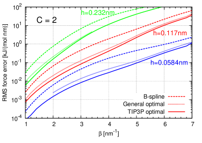
Figure 4: The RMS reciprocal force error of the B-spline (dashed lines), the general optimal (dotted lines) and the TIP3P optimal (solid lines) bases plotted against the splitting parameter in the TIP3P water system. The force scheme is the analytical differentiation, and the basis truncation is $C=2$. The green, red and blue lines present the mesh spacings of 0.234, 0.117 and 0.0584 nm, respectively.

Taking the TIP3P water system as an example, we numerically compare the basis that optimizes the homogeneity error and the basis that optimizes the estimated error including the charge correlation, i.e. Eq. (32). The former basis is model-independent, while the latter is model specific, thus we refer to them as the general optimal basis and the TIP3P optimal basis, respectively. In Fig. 4, we present the accuracy of the B-spline basis (dashed lines), the general optimal basis (dotted lines) and the TIP3P optimal basis (solid lines). The basis truncation was set to $C=2$ for all cases. The force scheme is analytical differentiation. The green, red and blue lines represent the errors of the mesh spacing $h=0.234$, 0.117 and 0.0584 nm, respectively. The general bases were optimized for different splitting parameter $\beta$ at $h=0.117$ nm, and were transferred to other mesh spacings if the products $\beta h$ are the same. The TIP3P optimal bases were optimized for all the investigated combinations of the splitting parameter and mesh spacing. It is observed that the TIP3P optimal basis is more accurate compared with the general optimal basis, and the advantage is more obvious for a smaller mesh spacing. Taking $\beta=3.0\ \textrm{nm}^{-1}$ for example, the TIP3P optimal basis reduces the error by 13%, 34% and 39% compared with the general optimal basis at mesh spacings $h=0.234$, 0.117 and 0.0584 nm, respectively. It should be noted that the cost of better accuracy is the model generality. The TIP3P optimal basis is specifically optimal for the TIP3P water system or systems dominated by the TIP3P water. It is not guaranteed that the TIP3P optimal basis is also optimal for other water models or other molecular systems with different charge correlations. In these systems, if the model specific optimal basis is not available, the general optimal basis is recommended.

VII Conclusion

In this manuscript, the optimal particle-mesh interpolation basis that minimizes the estimated RMS force error is proposed for the fast Ewald method. It is demonstrated that the optimal basis achieves significantly higher accuracy than the widely used B-spline basis for both the ik- and analytical differentiation force schemes, at a cost of marginally (less than $5\%$) longer computational time. We prove that the optimal basis is system independent, and is determined by a characteristic number that is the product of the splitting parameter and the mesh spacing. Therefore, it is convenient to build a database of the general optimal bases and to integrate them into existing MD packages. By taking into account the charge correlation, the accuracy of the optimal basis is further improved. However, the cost of this improvement is the generality. We show that the optimal basis derived in this way is specific to a molecular model, and should be optimized for all possible combinations of the splitting parameter and mesh spacing. Therefore, the choice between the general optimal basis and the model specific optimal basis is a trade-off between the generality and the accuracy.

Appendix A The cubic Hermite splines

The cubic Hermite splines $H_{00}$, $H_{01}$, $H_{10}$ and $H_{11}$ are defined, on the interval $u\in[0,1]$, by

$$H_{00}(u) =(1+2u)(1-u)^{2},$$ (38)

$$H_{01}(u) =u^{2}(3-2u),$$ (39)

$$H_{10}(u) =u(1-u)^{2},$$ (40)

$$H_{11}(u) =u^{2}(u-1).$$ (41)

It can be easily shown that

$$H_{00}(0) =1,\quad H_{00}(1)=H^{\prime}_{00}(0)=H^{\prime}_{00}(1)=0,$$ (42)

$$H_{01}(1) =1,\quad H_{01}(0)=H^{\prime}_{01}(0)=H^{\prime}_{01}(1)=0,$$ (43)

$$H^{\prime}_{10}(0) =1,\quad H_{10}(0)=H_{10}(1)=H^{\prime}_{10}(1)=0,$$ (44)

$$H^{\prime}_{11}(1) =1,\quad H_{11}(0)=H_{11}(1)=H^{\prime}_{11}(0)=0.$$ (45)

Therefore, the ansatz functions $\eta_{i}(x)$ and $\theta_{i}(x)$ defined by Eq. (25)–(27) are supported on the interval $x\in[x_{i-1},x_{i+1}]$, and have the following properties:

$$\eta_{i}(x_{i})=1,\quad\eta_{i}(x_{i-1})=\eta_{i}(x_{i+1})=0,$$ (46)

$$\eta^{\prime}_{i}(x_{i-1})=\eta^{\prime}_{i}(x_{i})=\eta^{\prime}_{i}(x_{i+1})=0,$$ (47)

$$\theta_{i}(x_{i-1})=\theta_{i}(x_{i})=\theta_{i}(x_{i+1})=0,$$ (48)

$$\theta^{\prime}_{i}(x_{i})=1,\quad\theta^{\prime}_{i}(x_{i-1})=\theta^{\prime}_{i}(x_{i+1})=0.$$ (49)

Therefore, the interpolation basis given by Eq. (24) has the properties:

$$\varphi(0)=1,\quad\varphi(C)=0,$$ (50)

$$\varphi^{\prime}(0)=\varphi^{\prime}(C)=0,$$ (51)

$$\varphi(x_{i})=\lambda_{i},$$ (52)

$$\varphi^{\prime}(x_{i})=\nu_{i}.$$ (53)

Appendix B Proof of the error estimate in the continuous form

For simplicity, we consider a simulation region of cuboid shape, and denote $L_{\alpha}=|\textbf{{a}}_{\alpha}|$, then $\textbf{{a}}_{\alpha}=L_{\alpha}\textbf{{e}}_{\alpha}$, where $\textbf{{e}}_{\alpha}$ is the unit vector on direction $\alpha$. In the reciprocal space, $\textbf{{a}}_{\alpha}^{\ast}=(1/L_{\alpha})\textbf{{e}}_{\alpha}$. The error estimate of the homogeneity error of the ik-differentiation is

$$|\mathcal{E}^{\mathrm{ik}}_{\mathrm{homo}}|^{2}=2q^{2}Q^{2}\sum_{\textbf{{m}}}\textbf{{G}}^{2}(\textbf{{m}})\sum_{\alpha,l\neq 0}\Big{|}\frac{\hat{\varphi}(m_{\alpha}+lK_{\alpha})}{\hat{\varphi}(m_{\alpha})}\Big{|}^{2}.$$ (54)

The summation on the r.h.s. can be considered as an approximation to the integration

$$|\mathcal{E}^{\mathrm{rec}}_{\mathrm{ik}}|^{2}=2q^{2}Q^{2}\int d\textbf{{m}}\textbf{{G}}^{2}(\textbf{{m}})\sum_{\alpha,l\neq 0}\Big{|}\frac{\hat{\varphi}(m_{\alpha}+lK_{\alpha})}{\hat{\varphi}(m_{\alpha})}\Big{|}^{2}.$$ (55)

We change the integration variable from $m_{\alpha}$ to $\mu_{\alpha}=m_{\alpha}/K_{\alpha}$, then the error estimate (55) becomes

$$|\mathcal{E}^{\mathrm{rec}}_{\mathrm{ik}}|^{2}=2q^{4}\int d\boldsymbol{\mu}NK_{1}K_{2}K_{3}\textbf{{G}}^{2}\Big{(}\sum_{\alpha}\mu_{\alpha}h^{-1}\textbf{{e}}_{\alpha}\Big{)}\sum_{\alpha,l\neq 0}\Big{|}\frac{\tilde{\varphi}(\mu_{\alpha}+l)}{\tilde{\varphi}(\mu_{\alpha})}\Big{|}^{2},$$ (56)

where we used the identity $Q^{2}=Nq^{2}$, and

$$\textbf{{m}}=\sum_{\alpha}m_{\alpha}\textbf{{a}}_{\alpha}^{\ast}=\sum_{\alpha}\mu_{\alpha}K_{\alpha}\frac{1}{L_{\alpha}}\textbf{{e}}_{\alpha}=\sum_{\alpha}\mu_{\alpha}h^{-1}\textbf{{e}}_{\alpha}.$$ (57)

In the last equation of (57), we assumed that the mesh spacing $h_{\alpha}=L_{\alpha}/K_{\alpha}$ is roughly the same on all directions, i.e. $h_{\alpha}\approx h$. The notation $\tilde{\varphi}$ in Eq. (56) is the Fourier transform of the interpolation basis represented by the new variable $\mu$:

$$\tilde{\varphi}(\mu)=\frac{1}{K}\int_{-C}^{C}\varphi(x)\ e^{-2\pi i\mu x}dx=\frac{1}{K}\int_{-K/2}^{K/2}\varphi(x)\ e^{-2\pi imx/K}dx=\hat{\varphi}(m).$$ (58)

In the second equation of (58), we noticed that the interpolation basis $\varphi$ is supported on $[-C,C]$. The function G is defined by

$$\textbf{{G}}(\textbf{{m}})=-\frac{2\mathrm{i}\textbf{{m}}}{V}\frac{\exp(-\pi^{2}\textbf{{m}}^{2}/\beta^{2})}{\textbf{{m}}^{2}},\quad|\textbf{{m}}|\neq 0.$$ (59)

It is easy to show that

$$NK_{1}K_{2}K_{3}\textbf{{G}}^{2}(\textbf{{m}})=\frac{4\rho}{h^{3}}\frac{\exp(-2\pi^{2}\textbf{{m}}^{2}/\beta^{2})}{\textbf{{m}}^{2}},\quad|\textbf{{m}}|\neq 0.$$ (60)

Inserting (60) into the error estimate (56) yields

$$|\mathcal{E}^{\mathrm{ik}}_{\mathrm{homo}}|^{2}=\frac{8\rho q^{4}\beta}{h^{3}\beta^{3}}\int d\boldsymbol{\mu}\frac{\exp(-2\pi^{2}|\boldsymbol{\mu}|^{2}/(\beta h)^{2})}{|\boldsymbol{\mu}|^{2}/(\beta h)^{2}}\sum_{\alpha,l\neq 0}\Big{|}\frac{\tilde{\varphi}(\mu_{\alpha}+l)}{\tilde{\varphi}(\mu_{\alpha})}\Big{|}^{2}.$$ (61)

The continuous error estimate (30) is proved. The continuous estimate of the homogeneity error of the analytical differentiation (31), and the estimates of the correlation errors of the ik- and analytical differentiations (36) and (37) can be proved analogously.

If we discretize the continuous form of the error estimate (61) by $K_{\alpha}$ discretization points on direction $\alpha$, we have, by replacing $d\mu_{\alpha}$ with $1/K_{\alpha}$ and $\mu_{\alpha}$ with $m_{\alpha}/K_{\alpha}$,

$$|\mathcal{E}^{\mathrm{ik}}_{\mathrm{homo}}|^{2}=\frac{8\rho q^{4}\beta}{h^{3}\beta^{3}}\sum\frac{1}{K_{1}K_{2}K_{3}}\frac{\exp(-2\pi^{2}|\sum(m_{\alpha}/K_{\alpha})\textbf{{e}}_{\alpha}|^{2}/(\beta h)^{2})}{|\sum(m_{\alpha}/K_{\alpha})\textbf{{e}}_{\alpha}|^{2}/(\beta h)^{2}}\sum_{\alpha,l\neq 0}\Big{|}\frac{\hat{\varphi}(m_{\alpha}+lK_{\alpha})}{\hat{\varphi}(m_{\alpha})}\Big{|}^{2},$$

where we have used Eq. (58). Noticing that $\textbf{{m}}=\sum m_{\alpha}/(hK_{\alpha})\textbf{{e}}_{\alpha}$ and the identity (60), the standard error estimate (54) is recovered. Therefore, the standard error estimate is the discretization of the integration in the continuous form, and the difference will vanish as the number of discretization nodes $K_{\alpha}$ goes to infinity.

References

- (1) D. van der Spoel and P.J. van Maaren. The origin of layer structure artifacts in simulations of liquid water. Journal of Chemical Theory and Computation, 2(1):1–11, 2006.
- (2) P. P. Ewald. Die berechnung optischer und elektrostatischer gitterpotentiale. Ann. Phys., 369(3):253–287, 1921.
- (3) EL Pollock and J. Glosli. Comments on p3m, fmm, and the ewald method for large periodic coulombic systems. Computer Physics Communications, 95(2-3):93–110, 1996.
- (4) S. Pronk, S. Páll, R. Schulz, P. Larsson, P. Bjelkmar, R. Apostolov, M.R. Shirts, J.C. Smith, P.M. Kasson, D. van der Spoel, B. Hess, and E. Lindahl. Gromacs 4.5: a high-throughput and highly parallel open source molecular simulation toolkit. Bioinformatics, page btt055, 2013.
- (5) J.C. Phillips, R. Braun, W. Wang, J. Gumbart, E. Tajkhorshid, E. Villa, C. Chipot, R.D. Skeel, L. Kale, and K. Schulten. Scalable molecular dynamics with namd. Journal of computational chemistry, 26(16):1781–1802, 2005.
- (6) S. Plimpton. Fast parallel algorithms for short-range molecular dynamics. Journal of Computational Physics, 117(1):1–19, 1995.
- (7) T. Darden, D. York, and L. Pedersen. Particle mesh ewald: An n· log (n) method for ewald sums in large systems. The Journal of Chemical Physics, 98:10089, 1993.
- (8) U. Essmann, L. Perera, M.L. Berkowitz, T. Darden, H. Lee, and L.G. Pedersen. A smooth particle mesh ewald method. The Journal of Chemical Physics, 103(19):8577, 1995.
- (9) R. W. Hockney and J. W. Eastwood. Computer Simulation Using Particles. IOP, London, 1988.
- (10) M. Deserno and C. Holm. How to mesh up ewald sums. i. a theoretical and numerical comparison of various particle mesh routines. The Journal of Chemical Physics, 109:7678, 1998.
- (11) F. Hedman and A. Laaksonen. Ewald summation based on nonuniform fast fourier transform. Chemical physics letters, 425(1-3):142–147, 2006.
- (12) Michael Pippig. Pfft: An extension of fftw to massively parallel architectures. SIAM Journal on Scientific Computing, 35(3):C213–C236, 2013.
- (13) M. Deserno and C. Holm. How to mesh up ewald sums. ii. an accurate error estimate for the particle–particle–particle-mesh algorithm. The Journal of Chemical Physics, 109:7694, 1998.
- (14) H. Wang, F. Dommert, and C. Holm. Optimizing working parameters of the smooth particle mesh ewald algorithm in terms of accuracy and efficiency. The Journal of chemical physics, 133:034117, 2010.
- (15) V. Ballenegger, J.J. Cerdà, and C. Holm. How to convert spme to p3m: influence functions and error estimates. Journal of Chemical Theory and Computation, 8:936–947, 2012.
- (16) H. Wang, P. Zhang, and C. Schütte. On the numerical accuracy of ewald, smooth particle mesh ewald, and staggered mesh ewald methods for correlated molecular systems. Journal of Chemical Theory and Computation, 8(9):3243–3256, 2012.
- (17) Franziska Nestler. Parameter tuning for the nfft based fast ewald summation. Frontier in Physics, 4, 2016.
- (18) Xingyu Gao, Jun Fang, and Han Wang. Kaiser-bessel basis for the particle-mesh interpolation. Physical Review E, 2017.
- (19) V Ballenegger, A Arnold, and JJ Cerda. Simulations of non-neutral slab systems with long-range electrostatic interactions in two-dimensional periodic boundary conditions. The Journal of chemical physics, 131(9):094107, 2009.
- (20) Simon W de Leeuw, John William Perram, and Edgar Roderick Smith. Simulation of electrostatic systems in periodic boundary conditions. i. lattice sums and dielectric constants. In Proceedings of the Royal Society of London A: Mathematical, Physical and Engineering Sciences, volume 373, pages 27–56. The Royal Society, 1980.
- (21) SW De Leeuw, JW Perram, and ER Smith. Simulation of electrostatic systems in periodic boundary conditions. ii. equivalence of boundary conditions. In Proceedings of the Royal Society of London A: Mathematical, Physical and Engineering Sciences, volume 373, pages 57–66. The Royal Society, 1980.
- (22) D. Frenkel and B. Smit. Understanding molecular simulation. Academic Press, Inc. Orlando, Fl, USA, 2010.
- (23) Han Wang, Xingyu Gao, and Jun Fang. Multiple staggered mesh ewald: Boosting the accuracy of the smooth particle mesh ewald method. Journal of Chemical Theory and Computation, 12:5596–5608, 2016.
- (24) R. Fletcher. Practical methods of optimization. 1987.
- (25) Davis E King. Dlib-ml: A machine learning toolkit. Journal of Machine Learning Research, 10(Jul):1755–1758, 2009.
- (26) William L Jorgensen, Jayaraman Chandrasekhar, Jeffry D Madura, Roger W Impey, and Michael L Klein. Comparison of simple potential functions for simulating liquid water. The Journal of chemical physics, 79(2):926–935, 1983.
- (27) Xingyu Gao, Jun Fang, and Han Wang. Sampling the isothermal-isobaric ensemble by langevin dynamics. The Journal of chemical physics, 144(12):124113, 2016.