Shot noise and biased tracers: a new look at the halo model

Abstract

Shot noise is an important ingredient to any measurement or theoretical modelling of discrete tracers of the large scale structure. Recent work has shown that the shot noise in the halo power spectrum becomes increasingly sub-Poissonian at high mass. Interestingly, while the halo model predicts a shot noise power spectrum in qualitative agreement with the data, it leads to an unphysical white noise in the cross halo-matter and matter power spectrum. In this work, we show that absorbing all the halo model sources of shot noise into the halo fluctuation field leads to meaningful predictions for the shot noise contributions to halo clustering statistics and remove the unphysical white noise from the cross halo-matter statistics. Our prescription straightforwardly maps onto the general bias expansion, so that the renormalized shot noise terms can be expressed as combinations of the halo model shot noises. Furthermore, we demonstrate that non-Poissonian contributions are related to volume integrals over correlation functions and their response to long-wavelength density perturbations. This leads to a new class of consistency relations for discrete tracers, which appear to be satisfied by our reformulation of the halo model. We test our theoretical predictions against measurements of halo shot noise bispectra extracted from a large suite of numerical simulations. Our model reproduces qualitatively the observed sub-Poissonian noise, although it underestimates the magnitude of this effect.

I Introduction

Measurements of the distribution of discrete tracers of the large scale structure are affected by cosmic variance and shot noise. While sampling variance has been studied thoroughly, shot noise has received less attention because, until recently, the Poissonian approximation was sufficient to deal with fairly noisy data. However, ongoing and upcoming surveys like DES, Euclid or LSST will reduce the statistical uncertainties down to a regime where deviations from Poisson noise become relevant, and could also be exploited (see, e.g., Seljak, Hamaus & Desjacques (2009); Hamaus et al. (2010); Hamaus, Seljak & Desjacques (2011, 2012); Yoo et al. (2012); Biagetti et al. (2013); Ferraro & Smith (2015); de Putter & Doré (2017)). In fact, deviations from Poisson noise in the clustering of galaxies and clusters have already been reported Paech et al. (2016).

Early work from Casas-Miranda et al. (2002); Seljak, Hamaus & Desjacques (2009) furnished evidence that massive halos have sub-Poissonian noise. This effect was thoroughly explored in Hamaus et al. (2010), who studied the eigenvalues of the halo shot noise stochasticity matrix or power spectrum $P_{\epsilon\epsilon}(k)$ as a function of halo mass $M$. Furthermore, Hamaus et al. (2010) proposed a simple analytic expression for the deviation of Poisson noise based on the halo model. The halo model (see Cooray & Sheth, 2002, for a review) provides an analytical framework, which enables us to describe the clustering of dark matter and galaxies from the spatial distribution and properties of dark matter halos Seljak (2000); Peacock & Smith (2000); Scoccimarro et al. (2001). However, while Hamaus et al. (2010) showed that the halo model reproduces reasonably well the properties of the halo shot noise power spectrum $P_{\epsilon\epsilon}(k)$, the model predicts an unphysical white noise in the cross halo-matter and matter-matter power spectrum $P_{h\delta}(k)$ and $P_{\delta\delta}(k)$, respectively Seljak (2000); Cooray & Sheth (2002); Tinker et al. (2005); Hamaus et al. (2010).

How to cure these inconsistencies is still an open question (see Scoccimarro et al. (2001) for early insights), although Smith, Desjacques & Marian (2011) already noticed that taking into account halo exclusion can cancel the white-noise contribution in the matter power spectrum. Ref.Baldauf et al. (2013) argued that the correct, physical explanation for the halo sub-Poissonian noise is halo exclusion (which, to some extent, is the reason for nonlinear bias). Using peak theory, which has built-in small-scale exclusion, they showed that halo exclusion alone reproduces the measurements of Hamaus et al. (2010). Unfortunately, it is difficult to extract predictions from peak theory etc. because small-scale exclusion is, by definition, a highly non-perturbative effect. An alternative consists in enforcing mass-momentum conservation as in Schmidt (2016). This procedure removes, by definition, all the unphysical terms, yet it does not uniquely constrain the form of the halo shot noise covariances.

Rather than attempting to model halo exclusion from first principles, this paper attempts to retain the simplicity of the halo model. More precisely, following a brief overview in §II of basic theoretical results, we explain in §III how the various sources of shot noise in the halo model should be re-organized such as to preserve the good agreement with the measurements of Hamaus et al. (2010) and, simultaneously, remove all the unphysical white noises from the theoretical predictions. Next, we demonstrate in §IV that it is possible to map this new halo model onto the general bias expansion, and obtain quantitative, unambiguous predictions for the renormalized shot noises. Furthermore, we outline in §V the consistency relations that exist between shot noise contributions and volume integrals over correlation functions. Finally, in §VI, we set out to measure bispectrum statistics of the halo shot noise using N-body simulations, and compare the numerical data with the predictions of our halo model approach. After a brief discussion of optimal weights and implementation of halo distribution occupations in §VII, we conclude in §VIII.

II Noise in perturbative bias expansions

At second order (which is enough for the purpose of this work), the generalized bias expansion takes the form (see Desjacques, Jeong & Schmidt (2016) for a review)

$$\delta_{h}(\textbf{\em x}) =b_{1}\delta(\textbf{\em x})+b_{\nabla^{2}\delta}\nabla^{2}\delta(\textbf{\em x})+\epsilon_{0}(\textbf{\em x})$$ (1)

$$\quad+\frac{1}{2}b_{2}\delta^{2}(\textbf{\em x})+b_{K^{2}}\big{(}K_{ij}^{2}\big{)}(\textbf{\em x})+\epsilon_{\delta}(\textbf{\em x})\delta(\textbf{\em x})\;,$$

upon neglecting some higher-derivative terms (such as $(\nabla\delta)^{2}(\textbf{\em x})$ etc.). All the fields on the right-hand side of this equation are non-linear and include fluctuations at all scales, except for the long mode, which can be reabsorbed into an effective cosmology. This will be essential to the discussion in §V.3. The coefficients $b_{1}$ and $b_{2}$ are the (Eulerian) linear and quadratic LIMD (local-in-matter-density, see Desjacques, Jeong & Schmidt (2016)) bias parameters, $b_{\nabla^{2}\delta}$ is a first-order higher-derivative bias, and $b_{K_{2}}$ is the second-order bias associated with the (traceless) tidal shear tensor $K_{ij}$ (also known as tidal shear bias). All these bias parameters sensitively depend on the halo mass $M$. Furthermore, products of fluctuation fields (the equivalent of composite operators) are renormalized, although our notation does not make it explicit. The linear term $\epsilon_{0}(\textbf{\em x})$ is the usual white noise in the limit $k\to 0$ considered in Dekel & Lahav (1999), whereas the second-order term $\epsilon_{\delta}\delta$ represents the response of the halo shot noise to a long-wavelength density perturbation Schmidt (2016). No less importantly, the noise fields $\epsilon_{0}$ and $\epsilon_{\delta}$ are uncorrelated with density fluctuations, i.e. $\langle\epsilon_{0}\delta\rangle=\langle\epsilon_{\delta}\delta\rangle=0$. However, as we shall see later, they are not fully specified by their 1-point statistics owing to small-scale exclusion, which introduces correlations on the scale of dark matter halos. At lowest order in perturbation theory, $\epsilon_{0}$ solely contributes to the halo auto-power spectrum and bispectrum, whereas the cross-correlation between $\epsilon_{0}$ and $\epsilon_{\delta}$ is relevant to the cross halo-matter bispectrum.

Namely, for the Gaussian initial conditions considered throughout this paper, the halo-matter auto- and cross-bispectra which we shall (indirectly) measure in the N-body simulations (cf. Sec.§VI) are reasonably described by the tree-level expressions (see in particular Peebles, 1980; Matarrese, Verde & Heavens, 1997; Scoccimarro, 2000; Pollack, Smith & Porciani, 2012; Desjacques, Jeong & Schmidt, 2016, for the shot noise contributions)

$$B_{hhh} =B_{\epsilon_{0}\epsilon_{0}\epsilon_{0}}^{\{0\}}+b_{1}^{3}B_{\delta\delta\delta}+\bigg{\{}b_{1}^{2}\bigg{[}b_{2}+2b_{K^{2}}\left(\mu_{23}^{2}-\frac{1}{3}\right)\bigg{]}P_{\text{lin}}(k_{2})P_{\text{lin}}(k_{3})+\mbox{(2 cyc.)}\bigg{\}}$$ (2)

$$B_{hh\delta} =\Big{[}P_{\epsilon_{0}\epsilon_{\delta}}(k_{1})+P_{\epsilon_{0}\epsilon_{\delta}}(k_{2})\Big{]}P_{\text{lin}}(k_{3})+b_{1}^{2}B_{\delta\delta\delta}+\bigg{\{}b_{1}\bigg{[}b_{2}+2b_{K^{2}}\left(\mu_{23}^{2}-\frac{1}{3}\right)\bigg{]}P_{\text{lin}}(k_{2})P_{\text{lin}}(k_{3})+\mbox{(2$\longleftrightarrow$3)}\bigg{\}}$$

$$B_{h\delta\delta} =b_{1}B_{\delta\delta\delta}+\bigg{[}b_{2}+2b_{K^{2}}\left(\mu_{23}^{2}-\frac{1}{3}\right)\bigg{]}P_{\text{lin}}(k_{2})P_{\text{lin}}(k_{3})\;,$$

where $P_{\text{lin}}(k)$ is the linear density power spectrum, and

$$B_{\delta\delta\delta} =2\left[\frac{5}{7}+\frac{1}{2}\mu_{12}\bigg{(}\frac{k_{1}}{k_{2}}+\frac{k_{2}}{k_{1}}\bigg{)}+\frac{2}{7}\mu_{12}^{2}\right]$$ (3)

$$\qquad\times P_{\text{lin}}(k_{1})P_{\text{lin}}(k_{2})+\mbox{(2 cyc.)}$$

is the tree-level matter bispectrum induced by the gravitational coupling of Fourier modes Peebles (1980). Here, $\mu_{12}$ is the cosine of the angle between $\textbf{\em k}_{1}$ and $\textbf{\em k}_{2}$.

We have not explicitly written the white noise contribution $B_{\epsilon_{0}\epsilon_{0}\delta}^{\{0\}}$ to $B_{hh\delta}$, $B_{\epsilon_{0}\delta\delta}^{\{0\}}$ to $B_{h\delta\delta}$ etc. since they must vanish on the ground that shot noise is uncorrelated with the density field. However, as we shall see below, the halo model yields $B_{\epsilon_{0}\epsilon_{0}\delta}^{\{0\}}\neq 0$ for instance. Let us also emphasize that all the noise covariances must converge to their Poissonian expectation in the regime $k_{i}\gg 1$ (i.e. for wavelengths much shorter than the typical size of a halo). For instance, $P_{\epsilon_{0}\epsilon_{0}}\to 1/\bar{n}$, $B_{\epsilon_{0}\epsilon_{0}\epsilon_{0}}\to 1/\bar{n}^{2}$. One also finds $P_{\epsilon_{0}\epsilon_{\delta}}\to 2b_{1}/\bar{n}$ Pollack, Smith & Porciani (2012); Schmidt (2016). However, in the regime $k_{i}\ll 1$ of interest for our paper, these noise covariances will generally differ from their Poisson expectation.

We will now illustrate the extent to which the halo model can be applied to infer quantitative estimates in the limit $k_{i}\to 0$.

III Shot-noise in the halo model

In the halo model, any polyspectra – i.e. power spectrum ($N=2$), bispectrum ($N=3$) – can be written as the sum of 1-halo, 2-halo, …, and $N$-halo contribution. This decomposition can be suitably extended to describe the clustering of dark matter halos themselves Scherrer & Bertschinger (1991); Smith, Scoccimarro & Sheth (2007); Hamaus et al. (2010). For sake of completeness, a selected collection of formulae useful to our analysis is listed in Appendix §A.

After stating our definition of the halo noise we shall measure in simulations, we briefly review in §III.2 how the white noise contribution to the halo power spectrum arises from 1-halo terms. Next, in §III.3 we scrutinize the shot noise in bispectrum statistics and show that the leading order contributions to the noise arise either from 1-halo or 2-halo terms depending on whether one considers auto- or cross- halo-matter bispectra.

III.1 Halo noise: definition

We define the halo noise fluctuation field $\epsilon_{i}$ of a given halo mass bin $i$ as

$$\epsilon_{i}(\textbf{\em k}) \equiv\delta_{i}(\textbf{\em k})-b_{i}\delta(\textbf{\em k})$$ (4)

$$=\epsilon_{0i}(\textbf{\em k})-b_{\nabla^{2}\delta i}k^{2}\delta(\textbf{\em k})$$

$$\quad+\frac{1}{2}b_{2i}(\delta^{2})(\textbf{\em k})+b_{K^{2}i}(K_{ij}^{2})(\textbf{\em k})+(\epsilon_{\delta i}\delta)(\textbf{\em k})+\dots$$

where $\delta_{i}(\textbf{\em k})$ and $\delta(\textbf{\em k})$ are the Fourier mode of the halo and matter density field, respectively, $(\delta^{2})(\textbf{\em k})$ is the Fourier transform of $\delta^{2}$ etc. This is the quantity whose 2- and 3-point statistics we shall extract from N-body simulations (see §VI). Note that, since all the products of fluctuation fields have been renormalized, a constant white noise contribution in the limit $k\to 0$ can only stem from a non-vanishing $P_{\epsilon_{0}\epsilon_{0}}(k\to 0)$ (which includes the $b_{2}^{2}$ 1-loop term etc.).

Note that our definition Eq.(4) of the halo noise is different from that of Hamaus, Seljak & Desjacques (2011). While we expect analyzes with different definitions to agree at large scales, the scale-dependence of the measured halo noise is fairly sensitive to the details of the definition adopted.

III.2 Power spectrum

The power spectrum of the halo shot noise (or shot noise covariance) is defined as Hamaus et al. (2010)

$$P_{\epsilon_{i}\epsilon_{j}}(k)\equiv\langle\epsilon_{i}(\textbf{\em k})\epsilon_{j}(-\textbf{\em k})\rangle^{\prime}\;,$$ (5)

where the prime indicates that we have removed a factor of $(2\pi)^{3}\delta^{D}(\textbf{\em k}_{1}+\textbf{\em k}_{2})$. The shot noise power spectrum thus reads Hamaus et al. (2010)

$$P_{\epsilon_{i}\epsilon_{j}}(k) =\langle\delta_{i}\delta_{j}\rangle(k)-b_{i}\langle\delta_{j}\delta\rangle(k)$$ (6)

$$\qquad-b_{j}\langle\delta_{i}\delta\rangle(k)+b_{i}b_{j}\langle\delta\delta\rangle(k)$$

$$=P_{ij}(k)-b_{i}P_{j\delta}(k)-b_{j}P_{i\delta}(k)+b_{i}b_{j}P_{\delta\delta}(k)\;.$$

The contribution from higher-order terms in the bias expansion Eq.(1) (such as $b_{2}\delta^{2}$) becomes relevant on mildly nonlinear scales. Since our focus is on large scales, we shall ignore them in what follows.

In the halo model framework, power spectra decompose into the sum of a 1-halo and a 2-halo term, i.e. $P_{XY}(k)\equiv P_{XY}^{\text{1H}}(k)+P_{XY}^{\text{2H}}(k)$, where $X$, $Y$ can be any fluctuation field (i.e. matter, halo, galaxy etc.). Since

$$P_{ij}^{\text{2H}}(k) \propto b_{i}b_{j}P_{\text{lin}}(k)$$ (7)

$$P_{i\delta}^{\text{2H}}(k) \propto b_{i}P_{\text{lin}}(k)$$

$$P_{\delta\delta}^{\text{2H}}(k) \propto P_{\text{lin}}(k)\;,$$

the 2-halo contributions are negligible relative to the 1-halo terms for $k\ll 1$. Consequently, shot noise in the limit $k\to 0$ arises exclusively from the 1-halo terms. For the cross power spectra of halos and matter, these are

$$P^{\text{1H}}_{ij}(k)\stackrel{{\scriptstyle k\to 0}}{{=}}\frac{1}{\bar{n}_{i}\bar{n}_{j}}\int\!dM\,n(M)\Theta(M,M_{i})\Theta(M,M_{j})\equiv\frac{\delta^{K}_{ij}}{\bar{n}_{i}}$$

$$P^{\text{1H}}_{i\delta}(k)\stackrel{{\scriptstyle k\to 0}}{{=}}\frac{1}{\bar{n}_{i}\bar{\rho}_{m}}\int\!dM\,Mn(M)\Theta(M,M_{i})\equiv\frac{\overline{M_{i}}}{\bar{\rho}_{m}}$$

$$P^{\text{1H}}_{\delta\delta}(k)\stackrel{{\scriptstyle k\to 0}}{{=}}\frac{1}{\bar{\rho}_{m}^{2}}\int\!dM\,M^{2}n(M)\equiv\frac{\langle nM^{2}\rangle}{\bar{\rho}_{m}^{2}}$$ (8)

upon taking the large-scale limit for the Fourier transform $u$ of the halo profile, i.e. $u(k\to 0|M)=1$. Here, $P_{i\delta}$ denotes the cross-power spectrum between the dark matter and the $i$th halo density field $\delta_{i}$, while $P_{ij}$ is the cross-power spectrum between the $i$th and $j$th halo fluctuation field $\delta_{i}$ and $\delta_{j}$. The latter formally reads

$$\delta_{i}(\textbf{\em x})=\frac{n_{i}(\textbf{\em x})}{\bar{n}_{i}}-1\;.$$ (9)

Furthermore, $\Theta(M,M_{i})$ is a combination of step functions which returns unity when $M$ lies within the mass bin centered at $M_{i}$, and zero otherwise. $n(M)$ is the number density of halos in the mass range $[M,M+dM]$ or halo mass function (and thus has units of inverse Mass$\cdot$Volume), so that

$$\bar{n}_{i}=\int\!dM\,n(M)\Theta(M,M_{i})$$ (10)

is the number density of halos in the $i$th bin. Note that our notation distinguishes between averages like

$$\overline{M_{i}^{k}b_{i}^{l}}\equiv\frac{1}{\bar{n}_{i}}\int\!dM\,M^{k}n(M)b_{1}^{l}(M)\Theta(M,M_{i})$$ (11)

over a single mass bin, which are indicated with an overline, and averages like

$$\langle nM^{k}b_{1}^{l}\rangle\equiv\int\!dM\,M^{k}n(M)b_{1}^{l}(M)$$ (12)

over all halos, which are denoted with the brackets $\langle...\rangle$. In practice, we choose a finite lower bound (e.g. equal to the mass of one dark matter particle in the numerical simulations) to avoid numerical instabilities at low mass. We have found that numerical estimates of $\langle nM^{k}b_{1}^{l}\rangle$ are not very sensitive to the lower limit of the integral. Finally, $\delta^{K}_{ij}$ is a Kronecker symbol, i.e. $\delta_{ij}^{K}=1$ if $i=j$ and zero otherwise.

Substituting the 1-halo contributions Eq.(8) into Eq.(6), the $k\to 0$ limit of halo noise power spectrum predicted by the halo model reads Hamaus et al. (2010):

$$P_{\epsilon_{i}\epsilon_{j}}(k\to 0) \equiv P_{\epsilon_{0i}\epsilon_{0j}}^{\{0\}}$$ (13)

$$=\frac{1}{\bar{n}_{i}}\delta_{ij}^{K}-b_{i}\frac{\overline{M_{j}}}{\bar{\rho}_{m}}-b_{j}\frac{\overline{M_{i}}}{\bar{\rho}_{m}}+b_{i}b_{j}\frac{\langle nM^{2}\rangle}{\bar{\rho}_{m}^{2}}\;.$$

For the same halo mass bin ($i=j$), we get

$$P_{\epsilon_{0}\epsilon_{0}}^{\{0\}}=\frac{1}{\bar{n}}\bigg{\{}1-2b_{1}\left(\frac{\bar{n}\overline{M}}{\bar{\rho}_{m}}\right)+b_{1}^{2}\left(\frac{\bar{n}\langle nM^{2}\rangle}{\bar{\rho}_{m}^{2}}\right)\bigg{\}}$$ (14)

Interestingly, Eq.(13) turns out to be in very good agreement with the numerical data as shown in Hamaus et al. (2010), although some of the halo model predictions are unphysical. Namely, there is no shot noise in the cross halo-mass power spectrum as this is nothing but the average density profile. Therefore, we should have $P_{i\delta}^{\text{1H}}\to 0$ in the limit $k\to 0$. Nonetheless, the halo model assumes

$$\langle\epsilon_{i}\delta\rangle\to\frac{\overline{M_{i}}}{\bar{\rho}_{m}}\neq 0\;,$$ (15)

where $\bar{\rho}_{m}$ is the average matter density in the Universe.

Similarly, we would also expect $P_{\delta\delta}^{\text{1H}}\to 0$ in the “thermodynamic” limit $m_{\text{DM}}\to 0$, where $m_{\text{DM}}$ is the mass of the dark matter particles. However, the halo model predicts $P_{\delta\delta}^{\text{1H}}\to\langle nM^{2}\rangle/\bar{\rho}_{m}^{2}$, a value noticeably larger than the Poisson $1/\bar{n}_{\text{DM}}$ (where $\bar{n}_{\text{DM}}$ is the number density of DM particles) observed in numerical simulations Cooray & Sheth (2002); Smith et al. (2003); Crocce & Scoccimarro (2008); Hamaus et al. (2010). These are only two among infinitely many examples for which the halo model does not yield physically consistent results.

Finally, standard implementations of the halo model ignore the possibility that the shot noise may not be Poissonian in the halo power spectrum, although there is evidence that this is not the case Casas-Miranda et al. (2002); Seljak, Hamaus & Desjacques (2009); Hamaus et al. (2010). We will show in §IV how these issues can be resolved all at once.

III.3 Bispectrum

Let us now turn to the bispectrum. Since we shall need cross-bispectra of different fluctuation fields, it is convenient to define the bispectrum of three fluctuation fields $X(\textbf{\em k}_{1})$, $Y(\textbf{\em k}_{2})$ and $Z(\textbf{\em k}_{3})$ as

$$B_{XYZ}(k_{1},k_{2},k_{3})\equiv\langle X(\textbf{\em k}_{1})X(\textbf{\em k}_{2})Y(\textbf{\em k}_{3})\rangle^{\prime}\;,$$ (16)

where, again, the “ ’ “attached to Fourier space correlators signifies that we have removed a factor of $(2\pi)^{3}\delta^{D}\!(\textbf{\em k}_{1}+\textbf{\em k}_{2}+\textbf{\em k}_{3})$ owing to the invariance under translations ($\delta^{D}$ is the Dirac distribution). In the halo model, bispectra can be written as a sum of a 1-, 2- and 3-halo term. To avoid clutter, we will often omit the explicit dependence of $B$ on the wavenumbers $k_{i}$. However, one should bear in mind that the wavenumbers are always ordered with the fluctuation fields as in Eq.(16).

Unlike power spectra, for which tree-level shot noise contributions can arise only through 1-halo terms, for bispectra these can arise either through the 1-halo or 2-halo terms.

To illustrate this point, let us begin with the bispectrum $B_{\epsilon_{i}\epsilon_{j}\epsilon_{k}}=\langle\epsilon_{i}(\textbf{\em k}_{1})\epsilon_{j}(\textbf{\em k}_{2})\epsilon_{k}(\textbf{\em k}_{3})\rangle^{\prime}$ of the halo noise fluctuation field $\epsilon_{i}$,

$$B_{\epsilon_{i}\epsilon_{j}\epsilon_{k}} =\langle\delta_{i}\delta_{j}\delta_{k}\rangle^{\prime}-\Big{[}b_{i}\langle\delta_{j}\delta_{k}\delta\rangle^{\prime}+\mbox{(2 cyc.)}\Big{]}+\Big{[}b_{i}b_{j}\langle\delta\delta\delta_{k}\rangle^{\prime}+\mbox{(2 cyc.)}\Big{]}-b_{i}b_{j}b_{k}\langle\delta\delta\delta\rangle^{\prime}$$

$$=\Big{.}B_{ijk}-b_{i}B_{\delta jk}-b_{j}B_{i\delta k}-b_{k}B_{ij\delta}+b_{k}b_{j}B_{i\delta\delta}+b_{i}b_{k}B_{\delta j\delta}+b_{i}b_{j}B_{\delta\delta k}-b_{i}b_{j}b_{k}B_{\delta\delta\delta}\;,$$ (17)

where, for shorthand convenience, $B_{ijk}$, $B_{ij\delta}$ etc. denote the halo bispectrum, the cross halo-matter bispectra etc. evaluated for the triplet of wavenumbers $(k_{1},k_{2},k_{3})$. The subscripts are ordered such that the first carries momentum $\textbf{\em k}_{1}$ and the third $\textbf{\em k}_{3}$.

$B_{\epsilon_{i}\epsilon_{j}\epsilon_{k}}$ contributes a white noise in the limit $k_{i}\to 0$, which we shall denote by $B_{\epsilon_{i}\epsilon_{j}\epsilon_{k}}^{\{0\}}$ (this corresponds to $B_{\epsilon}^{\{0\}}$ in the notation of Desjacques, Jeong & Schmidt (2016)). From the point of view of the halo model, since the various 2- and 3-halo contributions $B^{\text{2H}}$ and $B^{\text{3H}}$ are proportional to the linear power spectrum $P_{\text{lin}}$ and, thereby, vanish in the limit $k_{i}\to 0$. The only terms relevant to $B_{\epsilon_{i}\epsilon_{j}\epsilon_{k}}^{\{0\}}$ thus are the 1-halo bispectra. Explicit expressions at finite wavenumber can be found in Appendix §A. In the low-$k$ limit, these become

$$B^{\text{1H}}_{ijk}(k_{1},k_{2},k_{3})\stackrel{{\scriptstyle k_{i}\to 0}}{{=}}\frac{1}{\bar{n}_{i}\bar{n}_{j}\bar{n}_{k}}\int\!dM\,n(M)\Theta(M,M_{i})\Theta(M,M_{j})\Theta(M,M_{k})\equiv\frac{1}{\bar{n}_{i}^{2}}\delta^{K}_{ijk}$$

$$B^{\text{1H}}_{ij\delta}(k_{1},k_{2},k_{3})\stackrel{{\scriptstyle k_{i}\to 0}}{{=}}\frac{1}{\bar{n}_{i}\bar{n}_{j}\bar{\rho}_{m}}\int\!dM\,Mn(M)\Theta(M,M_{i})\Theta(M,M_{j})\equiv\frac{\overline{M_{i}}}{\bar{n}_{i}\bar{\rho}_{m}}\delta^{K}_{ij}$$

$$B^{\text{1H}}_{i\delta\delta}(k_{1},k_{2},k_{3})\stackrel{{\scriptstyle k_{i}\to 0}}{{=}}\frac{1}{\bar{n}_{i}\bar{\rho}_{m}^{2}}\int\!dM\,M^{2}n(M)\Theta(M,M_{i})\equiv\frac{\overline{M_{i}^{2}}}{\bar{\rho}_{m}^{2}}$$

$$B^{\text{1H}}_{\delta\delta\delta}(k_{1},k_{2},k_{3})\stackrel{{\scriptstyle k_{i}\to 0}}{{=}}\frac{1}{\bar{\rho}_{m}^{3}}\int\!dM\,M^{3}n(M)\equiv\frac{\langle nM^{3}\rangle}{\bar{\rho}_{m}^{3}}$$ (18)

Note that, for a halo abundance $\bar{n}_{i}\ll 1$, each of these 1-halo term is suppressed relative to $B^{\text{1H}}_{ijk}$ by a (dimensionless) factor of $(\bar{n}\overline{M}/\bar{\rho}_{m})^{k}$, where $k$ is the number of density field $\delta$. Substituting the halo model predictions Eq.(18) into the definition Eq.(17) of the halo noise bispectrum, we obtain

$$B_{\epsilon_{i}\epsilon_{j}\epsilon_{k}}(k_{i}\to 0) \equiv B_{\epsilon_{0i}\epsilon_{0j}\epsilon_{0k}}^{\{0\}}$$ (19)

$$=-b_{i}b_{j}b_{k}\frac{\langle nM^{3}\rangle}{\bar{\rho}_{m}^{3}}+\bigg{[}b_{i}b_{j}\frac{\overline{M_{k}^{2}}}{\bar{\rho}_{m}^{2}}+\mbox{(2 cyc.)}\bigg{]}$$

$$\qquad-\bigg{[}b_{i}\left(\frac{\overline{M_{j}}}{\bar{n}_{j}\bar{\rho}_{m}}\right)\delta_{jk}^{K}+\mbox{(2 cyc.)}\bigg{]}+\frac{\delta_{ijk}^{K}}{\bar{n}_{i}^{2}}\;.$$

The magnitude of $B_{\epsilon_{0i}\epsilon_{0j}\epsilon_{0k}}^{\{0\}}$ strongly depends on the number of identical noise field. When two or three noise fluctuation fields are different, it is suppressed by one or two factors of $\bar{n}\overline{M}/\bar{\rho}_{m}$ relative to the Poisson expectation $1/\bar{n}^{2}$. By contrast, when the three noise fluctuation fields are identical, we find

$$B_{\epsilon_{0}\epsilon_{0}\epsilon_{0}}^{\{0\}} =\frac{1}{\bar{n}^{2}}\bigg{\{}1-3b_{1}\left(\frac{\bar{n}\overline{M}}{\bar{\rho}_{m}}\right)$$ (20)

$$\qquad+3b_{1}^{2}\left(\frac{\bar{n}^{2}\overline{M^{2}}}{\bar{\rho}_{m}^{2}}\right)-b_{1}^{3}\left(\frac{\bar{n}^{2}\langle nM^{3}\rangle}{\bar{\rho}_{m}^{3}}\right)\bigg{\}}\;,$$

where all the parentheses within the curly brackets are dimensionless quantities

Eq.(20) furnishes a prediction for the zero-point amplitude of the shot noise bispectrum $B^{\{0\}}_{\epsilon_{0}\epsilon_{0}\epsilon_{0}}$. As we shall see in §VI, this prediction broadly agrees with measurements of the halo shot noise bispectrum extracted from a large suite of numerical simulations. However, Eq.(18) shows that the halo model predicts, among others, a constant white noise contribution $B_{ii\delta}\to(\overline{M}_{i}/\bar{n}_{i}\bar{\rho}_{m})\ll\bar{n}_{i}^{-2}$ in the limit $k_{i}\to 0$. Like for the cross halo-matter power spectrum $P_{i\delta}$, this contribution is unphysical because the matter fluctuation field is devoid of shot noise in the thermodynamic limit $m_{\text{DM}}\to 0$. Therefore, shot noise in $B_{ij\delta}$ can only arise from second- or higher-order contributions to $\epsilon_{i}$ which, at lowest order, are proportional to $P_{\text{lin}}(k_{i})$. In the halo model, terms linear in $P_{\text{lin}}$ arise from 2-halo terms.

The relevant 2-halo contributions are listed in Appendix §A. In the low-$k$ limit, they are given by

$$B^{\text{2H}}_{ij\delta}(k_{1},k_{2},k_{3}) \stackrel{{\scriptstyle k_{i}\to 0}}{{=}}\frac{1}{\bar{n}_{i}\bar{n}_{j}\bar{\rho}_{m}}\int\!dM\,\Theta(M,M_{i})n(M)b_{1}(M)\int\!dM^{\prime}\,\Theta(M^{\prime},M_{j})M^{\prime}n(M^{\prime})b_{1}(M^{\prime})P_{\text{lin}}(k_{1})$$

$$\qquad+\frac{1}{\bar{n}_{i}\bar{n}_{j}\bar{\rho}_{m}}\int\!dM\,\Theta(M,M_{j})n(M)b_{1}(M)\int\!dM^{\prime}\,\Theta(M^{\prime},M_{i})M^{\prime}n(M^{\prime})b_{1}(M^{\prime})P_{\text{lin}}(k_{2})$$

$$\qquad+\frac{1}{\bar{n}_{i}\bar{n}_{j}\bar{\rho}_{m}}\int\!dM\,Mn(M)b_{1}(M)\int\!dM^{\prime}\,\Theta(M^{\prime},M_{i})\Theta(M^{\prime},M_{j})n(M^{\prime})b_{1}(M^{\prime})P_{\text{lin}}(k_{3})$$

$$\quad\equiv b_{i}\frac{\overline{M_{j}b_{j}}}{\bar{\rho}_{m}}P_{\text{lin}}(k_{1})+b_{j}\frac{\overline{M_{i}b_{i}}}{\bar{\rho}_{m}}P_{\text{lin}}(k_{2})+\frac{b_{i}}{\bar{n}_{i}}\delta_{ij}^{K}P_{\text{lin}}(k_{3})$$

$$B^{\text{2H}}_{i\delta\delta}(k_{1},k_{2},k_{3}) \stackrel{{\scriptstyle k_{i}\to 0}}{{=}}\frac{1}{\bar{n}_{i}\bar{\rho}_{m}^{2}}\int\!dM\,\Theta(M,M_{i})n(M)b_{1}(M)\int\!dM^{\prime}\,(M^{\prime})^{2}n(M^{\prime})b_{1}(M^{\prime})P_{\text{lin}}(k_{1})$$

$$\qquad+\frac{1}{\bar{n}_{i}\bar{\rho}_{m}^{2}}\int\!dM\,Mn(M)b_{1}(M)\int\!dM^{\prime}\,\Theta(M^{\prime},M_{i})M^{\prime}n(M^{\prime})b_{1}(M^{\prime})\Big{[}P_{\text{lin}}(k_{2})+P_{\text{lin}}(k_{3})\Big{]}$$

$$\quad\equiv b_{i}\frac{\langle nM^{2}b_{1}\rangle}{\bar{\rho}_{m}^{2}}P_{\text{lin}}(k_{1})+\frac{\overline{M_{i}b_{i}}}{\bar{\rho}_{m}}\Big{[}P_{\text{lin}}(k_{2})+P_{\text{lin}}(k_{3})\Big{]}$$

$$B^{\text{2H}}_{\delta\delta\delta}(k_{1},k_{2},k_{3}) \stackrel{{\scriptstyle k_{i}\to 0}}{{=}}\frac{1}{\bar{\rho}_{m}^{3}}\int\!dM\,Mn(M)b_{1}(M)\int\!dM^{\prime}\,\big{(}M^{\prime}\big{)}^{2}n(M^{\prime})b_{1}(M^{\prime})P_{\text{lin}}(k_{3})+\mbox{(2 cyc.)}$$

$$\quad\equiv\frac{\langle nM^{2}b_{1}\rangle}{\bar{\rho}_{m}^{2}}P_{\text{lin}}(k_{3})+\mbox{(2 cyc.)}\;,$$ (21)

where the wavemode $k_{3}$ is always assigned to the last (density) fluctuation field. Furthermore, $\overline{M_{i}b_{i}}$ designates the average of the product $M\cdot b_{1}$ across one halo bin. To obtain the last equalities, we have extensively applied the relation

$$\int\!dM\,Mn(M)b_{1}(M)\equiv\bar{\rho}_{m}\;,$$ (22)

which follows from mass conservation and the peak-background split relation for the linear halo bias (see Desjacques, Jeong & Schmidt (2016) and references therein),

$$b_{1}=\frac{\bar{\rho}_{m}}{\bar{n}}\frac{\partial\bar{n}}{\partial\bar{\rho}_{m}}\;.$$ (23)

Substituting the 1-halo and 2-halo expressions (18) and (21) into the cross-bispectrum $B_{\epsilon_{i}\epsilon_{j}\delta}(k_{1},k_{2},k_{3})\equiv\langle\epsilon_{i}(\textbf{\em k}_{1})\epsilon_{j}(\textbf{\em k}_{2})\delta(\textbf{\em k}_{3})\rangle^{\prime}$ of halo noise and matter fluctuation fields,

$$B_{\epsilon_{i}\epsilon_{j}\delta}=\Big{.}B_{ij\delta}-b_{i}B_{\delta j\delta}-b_{j}B_{i\delta\delta}+b_{i}b_{j}B_{\delta\delta\delta}\;,$$ (24)

a naive application of the halo model yields

$$B_{\epsilon_{i}\epsilon_{j}\delta}(k_{i}\to 0) \equiv B_{\epsilon_{0i}\epsilon_{0j}\delta}^{\{0\}}$$ (25)

$$\qquad+\Big{(}P_{\epsilon_{0i}\epsilon_{\delta j}}^{\{0\}}+P_{\epsilon_{0j}\epsilon_{\delta i}}^{\{0\}}\Big{)}P_{\text{lin}}(k_{3})\;,$$

where

$$B_{\epsilon_{0i}\epsilon_{0j}\delta}^{\{0\}}=\frac{\overline{M_{i}}}{\bar{n}_{i}\bar{\rho}_{m}}\delta_{ij}^{K}-b_{i}\frac{\overline{M_{j}^{2}}}{\bar{\rho}_{m}^{2}}-b_{j}\frac{\overline{M_{i}^{2}}}{\bar{\rho}_{m}^{2}}+b_{i}b_{j}\frac{\langle nM^{3}\rangle}{\bar{\rho}_{m}^{3}}$$ (26)

is the white noise piece arising from the 1-halo terms. For the 2-halo piece, some cancellations occur and we are left with

$$P_{\epsilon_{0i}\epsilon_{\delta j}}^{\{0\}}+P_{\epsilon_{0j}\epsilon_{\delta i}}^{\{0\}} =\frac{b_{i}}{\bar{n}_{i}}\delta_{ij}^{K}-b_{i}\frac{\overline{M_{j}b_{j}}}{\bar{\rho}_{m}}-b_{j}\frac{\overline{M_{i}b_{i}}}{\bar{\rho}_{m}}$$ (27)

$$\qquad+b_{i}b_{j}\frac{\langle nM^{2}b_{1}\rangle}{\bar{\rho}_{m}^{2}}\;.$$

This is the amplitude proportional to $P_{\text{lin}}(k_{3})$ in the limit $k_{i}\ll 1$.

In the next Section, we shall argue that $B_{\epsilon_{0i}\epsilon_{0j}\delta}^{\{0\}}\equiv 0$, in contrast to Eq.(26), is the correct answer. However, we will also see that the prediction for the amplitude $P_{\epsilon_{0i}\epsilon_{\delta j}}^{\{0\}}+P_{\epsilon_{0j}\epsilon_{\delta i}}^{\{0\}}$ of the term proportional to $P_{\text{lin}}(k_{3})$ obtained from a brute force application of the halo model is physically sound. This amplitude is generally negative for $i\neq j$ whereas, in the particular case $i=j$, we find

$$P_{\epsilon_{0}\epsilon_{\delta}}^{\{0\}}=\frac{b_{1}}{2\bar{n}}\bigg{\{}1-2\left(\frac{\bar{n}\overline{Mb_{1}}}{\bar{\rho}_{m}}\right)+b_{1}\left(\frac{\bar{n}\langle nM^{2}b_{1}\rangle}{\bar{\rho}_{m}^{2}}\right)\bigg{\}}$$ (28)

The first term in the parenthesis yields the Poisson expectation (already derived in Pollack, Smith & Porciani (2012); Schmidt (2016)), which is expected to be valid in the limit $k\gg 1$ only. The other terms are the non-Poissonian corrections that arise from halo exclusion. Note that the non-Poissonian correction in Eq.(28) differ from that in Eq.(14) due to the position of a factor of $b_{1}$ in the third term.

The generalization of these calculations to higher-order polyspectra is straightforward. As a general rule, a naive application of the halo model will predict physically consistent noise covariances so long as they do not involve any density fluctuation field, and fail in all other cases.

IV Self-consistent treatment of shot noise in the halo model

In the previous Section, we have shown that the halo model can used to compute shot noise contribution beyond the constant white noise term scrutinized in the study of Hamaus et al. (2010). However, as we have already emphasized, some of the halo model predictions are unphysical. For bispectra for instance, there should not be any constant white noise in the limit $k_{i}\to 0$ unless the bispectrum is computed for three halo fluctuation fields. How can we avoid these inconsistencies and simultaneously retain the halo model predictions for $P_{\epsilon_{0}\epsilon_{0}}^{\{0\}}$ or $B_{\epsilon_{0}\epsilon_{0}\epsilon_{0}}^{\{0\}}$ which, as we shall see in §VI, are in reasonably good agreement with the data ?

To address this question, we begin by writing down a perturbative expansion for both the halo and matter overdensity fields that reproduces the “original” halo model predictions Eqs. (8), (21) and (18). In light of the bias expansion Eq.(1), we try to following ansatz:

$$\Big{.}\delta_{i}(\textbf{\em x}) =\big{(}b_{i}+\tilde{\epsilon}_{\delta i}(\textbf{\em x})\big{)}\delta(\textbf{\em x})+\tilde{\epsilon}_{0i}(\textbf{\em x})$$

$$\Big{.}\delta_{m}(\textbf{\em x}) =\big{(}1+\tilde{\epsilon}_{\delta m}(\textbf{\em x})\big{)}\delta(\textbf{\em x})+\tilde{\epsilon}_{0m}(\textbf{\em x})\;,$$ (29)

where we have ignored second- and higher-order terms. Here, $\delta$ should be interpreted as the noise-free, nonlinear density field, whereas $\tilde{\epsilon}_{\delta m}$ and $\tilde{\epsilon}_{0m}$ are the matter equivalents to the lowest order halo shot noise terms. In the halo model, they do not vanish even in the limit $m_{\text{DM}}\to 0$ considered throughout our calculations. For clarity, we use tilde in order to distinguish the halo shot noise contributions from the renormalized shot noise terms which appear in Eq.(1).

To assess the extent to which Eq.(29) reproduces the halo model predictions in the low-$k$ limit, we compute the large-scale 2-point and 3-point covariances of the noise fields $\tilde{\epsilon}_{0i}$, $\tilde{\epsilon}_{\delta i}$, $\tilde{\epsilon}_{0m}$ and $\tilde{\epsilon}_{0\delta}$ using our ansatz for the halo and matter fluctuation field $\delta_{h}(\textbf{\em x})$ and $\delta_{m}(\textbf{\em x})$ (which replaces $\delta(\textbf{\em x})$ for this consistency check), respectively. We consider first the 2-point covariances. The calculation of $\langle\delta_{h}\delta_{h}\rangle$, $\langle\delta_{h}\delta_{m}\rangle$ and $\langle\delta_{m}\delta_{m}\rangle$ in the limit $k\to 0$ is straightfoward. Upon identifying our results with Eq.(8), the following noise power spectra must satisfy:

$$P_{\tilde{\epsilon}_{0i}\tilde{\epsilon}_{0j}}^{\{0\}}=\frac{\delta_{ij}^{K}}{\bar{n}_{i}}\;,\quad P_{\tilde{\epsilon}_{0i}\tilde{\epsilon}_{0m}}^{\{0\}}=\frac{\overline{M_{i}}}{\bar{\rho}_{m}}\;,$$ (30)

$$P_{\tilde{\epsilon}_{0m}\tilde{\epsilon}_{0m}}^{\{0\}}=\frac{\langle\bar{n}M^{2}\rangle}{\bar{\rho}_{m}^{2}}\;.$$

Similarly, the 2-halo contribution to the various cross halo-matter bispectra $\langle\delta_{h}\delta_{h}\delta_{m}\rangle$ etc. in the limit $k_{i}\ll 1$, Eq.(21), constrain another set of 2-point covariances. Namely, terms proportional to $P_{\text{lin}}(k_{3})$ arise from 4-point correlators involving two shot noise and two density fields (5-point correlators of the form $\langle(\epsilon_{X}\delta)(\textbf{\em k}_{1})(\epsilon_{Y}\delta)(\textbf{\em k}_{2})\epsilon_{Z}(\textbf{\em k}_{3})\rangle$ return a loop). In the limit $k_{i}\to 0$, the relevant shot noise contributions are:

$$B_{mmm}(k_{1},k_{2},k_{3}) \supset\Big{[}P_{\tilde{\epsilon}_{\delta m}\tilde{\epsilon}_{0m}}(k_{1})+P_{\tilde{\epsilon}_{\delta m}\tilde{\epsilon}_{0m}}(k_{2})\Big{]}P_{\text{lin}}(k_{3})+\mbox{(2 cyc.)}$$ (31)

$$B_{imm}(k_{1},k_{2},k_{3}) \supset b_{i}\Big{[}P_{\tilde{\epsilon}_{\delta m}\tilde{\epsilon}_{0m}}(k_{2})+P_{\tilde{\epsilon}_{\delta m}\tilde{\epsilon}_{0m}}(k_{3})\Big{]}P_{\text{lin}}(k_{1})+\Big{[}P_{\tilde{\epsilon}_{\delta i}\tilde{\epsilon}_{0m}}(k_{3})+P_{\tilde{\epsilon}_{0i}\tilde{\epsilon}_{\delta m}}(k_{1})\Big{]}P_{\text{lin}}(k_{2})$$

$$\qquad+\Big{[}P_{\tilde{\epsilon}_{0i}\tilde{\epsilon}_{\delta m}}(k_{1})+P_{\tilde{\epsilon}_{\delta i}\tilde{\epsilon}_{0m}}(k_{2})\Big{]}P_{\text{lin}}(k_{3})$$

$$B_{ijm}(k_{1},k_{2},k_{3}) \supset b_{i}\Big{[}P_{\tilde{\epsilon}_{0j}\tilde{\epsilon}_{\delta m}}(k_{2})+P_{\tilde{\epsilon}_{\delta j}\tilde{\epsilon}_{0m}}(k_{3})\Big{]}P_{\text{lin}}(k_{1})+b_{j}\Big{[}P_{\tilde{\epsilon}_{\delta i}\tilde{\epsilon}_{0m}}(k_{3})+P_{\tilde{\epsilon}_{0i}\tilde{\epsilon}_{\delta m}}(k_{1})\Big{]}P_{\text{lin}}(k_{2})$$

$$\qquad+\Big{[}P_{\tilde{\epsilon}_{0i}\tilde{\epsilon}_{\delta j}}(k_{1})+P_{\tilde{\epsilon}_{\delta i}\tilde{\epsilon}_{0j}}(k_{2})\Big{]}P_{\text{lin}}(k_{3})\;.$$

Identifying the above expressions with Eq.(21), the following combination of zero-lag noise power spectra must satisfy

$$P_{\tilde{\epsilon}_{\delta m}\tilde{\epsilon}_{0m}}^{\{0\}}=\frac{\langle nM^{2}b_{1}\rangle}{2\bar{\rho}_{m}^{2}}\;,\quad P_{\tilde{\epsilon}_{\delta i}\tilde{\epsilon}_{0m}}^{\{0\}}+P_{\tilde{\epsilon}_{0i}\tilde{\epsilon}_{\delta m}}^{\{0\}}=b_{i}\frac{\overline{M_{i}}}{\bar{\rho}_{m}}\;,$$

$$P_{\tilde{\epsilon}_{\delta i}\tilde{\epsilon}_{0j}}^{\{0\}}+P_{\tilde{\epsilon}_{0i}\tilde{\epsilon}_{\delta j}}^{\{0\}}=\frac{b_{i}}{\bar{n}_{i}}\delta_{ij}^{K}\;.$$ (32)

Finally, some of the 3-point noise covariances can be read off from Eqs.(18). We find:

$$B_{\tilde{\epsilon}_{0i}\tilde{\epsilon}_{0j}\tilde{\epsilon}_{0k}}^{\{0\}}=\frac{1}{\bar{n}_{i}^{2}}\delta_{ijk}^{K}\;,\quad B_{\tilde{\epsilon}_{0i}\tilde{\epsilon}_{0j}\tilde{\epsilon}_{0m}}^{\{0\}}=\frac{\overline{M_{i}}}{\bar{n}_{i}\bar{\rho}_{m}}\delta_{ij}^{K}$$ (33)

$$B_{\tilde{\epsilon}_{0i}\tilde{\epsilon}_{0m}\tilde{\epsilon}_{0m}}^{\{0\}}=\frac{\overline{M_{i}^{2}}}{\bar{\rho}_{m}^{2}}\;,\quad B_{\tilde{\epsilon}_{0m}\tilde{\epsilon}_{0m}\tilde{\epsilon}_{0m}}^{\{0\}}=\frac{\langle nM^{3}\rangle}{\bar{\rho}_{m}^{3}}\;.$$

In particular, $B_{ijm}$ exhibits a constant white noise in the low-$k$ because $B_{\tilde{\epsilon}_{0i}\tilde{\epsilon}_{0j}\tilde{\epsilon}_{0m}}^{\{0\}}\neq 0$. All this suggests that the halo model indeed assumes that the halo and matter overdensity be described by perturbative expansions of the form Eq.(29).

In order to remedy the unphysical, large-scale behaviour of all the 1-halo terms involving at least one density field, and simultaneously retain the halo model predictions for $P_{\epsilon_{0i}\epsilon_{0j}}^{\{0\}}$, $P_{\epsilon_{0i}\epsilon_{\delta j}}^{\{0\}}$ etc., we argue that the halo model perturbative expansion Eq.(29) should be reorganized such that

$$\Big{.}\delta_{i}(\textbf{\em x}) =\big{(}b_{i}+\tilde{\epsilon}_{\delta i}(\textbf{\em x})-b_{i}\tilde{\epsilon}_{\delta m}(\textbf{\em x})\big{)}\delta(\textbf{\em x})$$ (34)

$$\qquad\Big{.}+\tilde{\epsilon}_{0i}(\textbf{\em x})-b_{i}\tilde{\epsilon}_{0m}(\textbf{\em x})$$

$$\Big{.}\delta_{m}(\textbf{\em x}) =\delta(\textbf{\em x})\;.$$

Here, $\delta(\textbf{\em x})$ is the nonlinear density field as in the pertubative bias expansion Eq.(1). At the tree-level considered in this paper, this ansatz clearly ensures that any correlator involving at least one matter fluctuation field does not exhibit a constant white noise in the limit $k_{i}\to 0$ (i.e., the right-hand side of Eq.(26) now vanishes). In particular,

$$\bigg{.}P_{i\delta}(k) \stackrel{{\scriptstyle k\ll 1}}{{=}}b_{i}P_{\text{lin}}(k)$$

$$\bigg{.}P_{\delta\delta}(k) \stackrel{{\scriptstyle k\ll 1}}{{=}}P_{\text{lin}}(k)$$ (35)

in the thermodynamics limit $m_{\text{DM}}\to 0$. At the same time, Eqs.(13), (19) and (27) are reproduced. This way, the halo model can be used to consistently predict the shot noise contributions that arise from the perturbative bias expansion Eq.(1) since we can identify the renormalized shot noises $\epsilon_{0}$ and $\epsilon_{\delta}$ with the halo model shot noises according to

$$\Big{.}\epsilon_{0i}(\textbf{\em x}) \equiv\tilde{\epsilon}_{0i}(\textbf{\em x})-b_{i}\tilde{\epsilon}_{0m}(\textbf{\em x})$$ (36)

$$\Big{.}\epsilon_{\delta i}(\textbf{\em x}) \equiv\tilde{\epsilon}_{\delta i}(\textbf{\em x})-b_{i}\tilde{\epsilon}_{\delta m}(\textbf{\em x})\;.$$

Eqs.(34) and (36) are the main results of this Section. They provide the building blocks for a self-consistent calculation of halo clustering statistics based on the halo model. We shall explore the extent to which our prescription generalizes to higher order in future work. For the moment, let us emphasize two important points.

Firstly, while the Poisson noise piece $\tilde{\epsilon}_{0i}(\textbf{\em x})$ has non-vanishing correlations at one-point only, e.g. $\langle\tilde{\epsilon}_{0i}(\textbf{\em x}_{1})\tilde{\epsilon}_{0j}(\textbf{\em x}_{2})\rangle\sim\delta^{D}\!(\textbf{\em x}_{1}-\textbf{\em x}_{2})$, the remaining auto- and cross-correlations are generally non-zero at separations $|\textbf{\em x}_{1}-\textbf{\em x}_{2}|\lesssim R_{\text{vir}}$, where $R_{\text{vir}}$ is the halo virial radius. This should be interpreted as a manifestation of halo exclusion, which introduces correlations at small scales. Therefore, the physical interpretation of Eq.(34) is that, while the matter distribution has zero shot noise in the limit $m_{\text{DM}}\to 0$ and, thus, satisfies the mass-momentum conservation, the halo shot noise is a combination of Poisson sampling noise and exclusion effects.

Secondly, a natural extension of our predictions to finite wavenumber would consist in replacing the covariances of the halo shot noises $\tilde{\epsilon}_{0i}$, $\tilde{\epsilon}_{\delta i}$ etc. by the halo model predictions at finite $k$. The 1-halo and 2-halo power spectra and bispectra relevant to the statistics considered in this paper are summarized in Appendix A. For instance, the covariance of $\epsilon_{0i}$ and $\epsilon_{0j}$ would read

$$P_{\epsilon_{0i}\epsilon_{0j}}(k) =\frac{\delta_{ij}^{K}}{\bar{n}_{i}}-b_{i}\frac{\overline{M_{j}}}{\bar{\rho}_{m}}u(k|M_{j})-b_{j}\frac{\overline{M_{i}}}{\bar{\rho}_{m}}u(k|M_{i})$$

$$\qquad+\frac{b_{i}b_{j}}{\bar{\rho}_{m}^{2}}\int\!dM\,M^{2}n(M)u(k|M)^{2}\;.$$ (37)

This expression has the correct limiting (Poissonian) behaviour in the limit $k\to\infty$. Furthermore, while the Poisson expectation does not depend on $k$ – which originates from $\langle\tilde{\epsilon}_{0i}(\textbf{\em x}_{1})\tilde{\epsilon}_{0j}(\textbf{\em x}_{2})\rangle\sim\delta^{D}\!(\textbf{\em x}_{1}-\textbf{\em x}_{2})$ – the non-Poissonian corrections involve the low-pass filter $u(k|M)$ since halo exclusion leads to correlations at separations less than the virial radius (In Lagrangian space, $u(k|M)$ would be replaced by the Lagrangian window function $W(k|M)$, see Baldauf et al. (2013)). It is beyond the scope of this paper to investigate the scale-dependence of the shot noise any further. However, we emphasize that any extension to finite wavenumber is straightforward only if the shot noise is uncorrelated with the density, i.e. $\langle\epsilon_{0}\delta\rangle=\langle\epsilon_{\delta}\delta\rangle=...=0$. This may not be the case if halo profiles retain memory of the initial conditions and the halo assembly history.

Before we discuss the implications of our results from a configuration space point of view, let us emphasize again that, although Eqs. (34) and (36) is a physically motivated ansatz, there is a priori no reason why it should furnish better predictions than that of, e.g., Schmidt (2016), who derived non-Poissonian expressions for $B_{\epsilon_{0i}\epsilon_{0j}\epsilon_{0k}}^{\{0\}}$ and $P_{\epsilon_{0i}\epsilon_{\delta j}}^{\{0\}}$ from the conservation of mass and momentum Peebles (1980). This raises the question as to whether there exist model-independent constraints on the shot noise contributions beyond the usual mass-momentum conservation invoked so far. We will argue in the forthcoming Section that this is indeed the case.

V Shot noise and volume integrals

In this Section, we outline a connection between Poissonian corrections and volume integrals over correlation functions. We demonstrate that, whenever certain volume integrals do not vanish, the noise is non-Poissonian. We also establish a correspondence between the squeezed limit of the cross halo-matter 3-point functions and the low-$k$ behaviour of the shot noise power spectrum $P_{\epsilon_{0}\epsilon_{\delta}}^{\{0\}}$, which can be generalized to a new class of consistency, or model-independent relations for biased tracers. Remarkably, our new halo model prescription, Eqs.(34) and (36), gives results consistent with all these expectations.

Before we proceed, let us emphasize that “volume integral” refers to the value of the following configuration space integrals:

$$\Xi_{i...k\delta...\delta}=\int\!d^{3}r_{1}\dots\int\!d^{3}r_{N}\,\xi_{i...k\delta...\delta}(\textbf{\em r}_{1},...,\textbf{\em r}_{N})\;,$$ (38)

where the $N$-point correlation function generically involves $k$ halo fields $\delta_{1}(\textbf{\em r}_{1})$, …, $\delta_{k}(\textbf{\em r}_{k})$ and $N-k$ matter fields $\delta(\textbf{\em r}_{k+1})$, …, $\delta(\textbf{\em r}_{N})$. Therefore, our discussion does not pertain to the “integral constraint” satisfied by correlation function estimators.

V.1 2-point correlation function

It is standard textbook result that the 2-point correlation of two discrete (homogeneous and isotropic) fluctuation fields takes the general form

$$\big{\langle}\delta_{i}(\textbf{\em x}_{1})\delta_{j}(\textbf{\em x}_{2})\big{\rangle}\equiv\frac{1}{\bar{n}_{i}}\delta_{ij}^{K}\delta^{D}\!(\textbf{\em r})+\xi_{ij}(r)\;,$$ (39)

where $r=|{\bf x}_{2}-{\bf x}_{1}|$. The first term in the right-hand side is the contribution from self-pairs. In the low-$k$ limit, the resulting power spectrum is

$$P_{ij}(k) =\frac{1}{\bar{n}_{i}}\delta_{ij}^{K}+\int\!d^{3}r\,\xi_{ij}(r)e^{-i\textbf{\em k}\cdot\textbf{\em r}}$$ (40)

$$\stackrel{{\scriptstyle k\ll 1}}{{=}}\left(\frac{1}{\bar{n}_{i}}\delta_{ij}^{K}+\Xi_{ij}\right)+b_{i}b_{j}P_{\text{lin}}(k)\;,$$

where

$$\Xi_{ij}\equiv\int\!\!d^{3}r\,\xi_{ij}(r)$$ (41)

is generally non-zero even when $i\neq j$ owing to small-scale exclusion effects Baldauf et al. (2013). This implies that cross-power spectra of two different tracer populations have non-zero shot noise contribution, as was pointed out in Hamaus et al. (2010). Furthermore, $\Xi_{ii}<0$ (resp. $\Xi_{ii}>0$) leads to sub-Poissonian (resp. super-Poissonian) shot noise. In Baldauf et al. (2013), $\Xi_{ij}$ is modelled using peak theory, which exhibits exclusion at small-scales. Alternatively, we can apply Eq.(36) to derive a physically consistent prediction for the non-Poissonian correction $\Xi_{ij}$. Namely, equating Eq.(13) (which follows from Eq.(36) and Eq.(40) gives

$$P_{\epsilon_{0i}\epsilon_{0j}}^{\{0\}}\equiv\frac{1}{\bar{n}_{i}}\delta_{ij}^{K}+\Xi_{ij}$$ (42)

and, consequently,

$$\Xi_{ij}\equiv-b_{i}\frac{\overline{M_{j}}}{\bar{\rho}_{m}}-b_{j}\frac{\overline{M_{i}}}{\bar{\rho}_{m}}+b_{i}b_{j}\frac{\langle nM^{2}\rangle}{\bar{\rho}_{m}^{2}}\;.$$ (43)

Note that $\overline{M_{i}}/\bar{\rho}_{m}$ is the Lagrangian volume occupied by the halo. In other words, it is along with the average $\langle nM^{k}\rangle$ etc., the manifestation of halo exclusion in our halo model framework. The last term ensures that a mass weighting of the halo distribution cancels out the noise in the limit where all halos are resolved (see Appendix §VII.1 for a details). Although only $b_{1}$ appears, it is pretty clear that higher-order bias has a strong influence on the shape of $\xi_{ij}(r)$, whence $\Xi_{ij}$. The effect of higher-order bias parameters is, to some extent, captured in the Lagrangian volume $\overline{M}/\bar{\rho}_{m}$. Finally, note also that, owing to $b_{1}$, a randomly distributed distribution of hard spheres with volume $\sim\overline{M}/\bar{\rho}_{m}$ would exhibit a different shot-noise correction than a similar, albeit clustered sample.

V.2 3-point correlation function

We now turn to the 3-point correlation function. With the aid of Eq.(9), we arrive at the well-known relations

$$\Big{\langle}\delta_{i}(\textbf{\em x}_{1})\delta_{j}(\textbf{\em x}_{2})\delta_{k}(\textbf{\em x}_{3})\Big{\rangle} =\xi_{ijk}(\textbf{\em r}_{12},\textbf{\em r}_{13})+\bigg{[}\frac{\delta_{ij}^{K}}{\bar{n}_{i}}\delta^{D}\!(\textbf{\em r}_{12})\xi_{ik}(\textbf{\em r}_{13})+\mbox{(2 cyc.)}\bigg{]}+\frac{\delta^{K}_{ijk}}{\bar{n}_{i}^{2}}\delta^{D}\!(\textbf{\em r}_{12})\delta^{D}\!(\textbf{\em r}_{13})$$

$$\Big{\langle}\delta_{i}(\textbf{\em x}_{1})\delta_{j}(\textbf{\em x}_{2})\delta(\textbf{\em x}_{3})\Big{\rangle} =\xi_{ij\delta}(\textbf{\em r}_{12},\textbf{\em r}_{13})+\frac{\delta_{ij}^{K}}{\bar{n}_{i}}\delta^{D}\!(\textbf{\em r}_{12})\xi_{i\delta}(\textbf{\em r}_{13})\;.$$ (44)

which, in Fourier space, become

$$B_{ijk}(k_{1},k_{2},k_{3}) =\int\!d^{3}r_{12}\int\!d^{3}r_{13}\,\xi_{ijk}(\textbf{\em r}_{12},\textbf{\em r}_{13})\,e^{-i\textbf{\em k}_{2}\cdot\textbf{\em r}_{12}-i\textbf{\em k}_{3}\cdot\textbf{\em r}_{13}}+\bigg{[}\frac{\delta_{ij}^{K}}{\bar{n}_{i}}\int\!d^{3}r\,\xi_{jk}(\textbf{\em r})\,e^{-i\textbf{\em k}_{3}\cdot\textbf{\em r}}+\mbox{(2 cyc.)}\bigg{]}+\frac{\delta_{ijk}^{K}}{\bar{n}_{i}^{2}}$$ (45)

$$B_{ij\delta}(k_{1},k_{2},k_{3}) =\int\!d^{3}r_{12}\int\!d^{3}r_{13}\,\xi_{ij\delta}(\textbf{\em r}_{12},\textbf{\em r}_{13})\,e^{-i\textbf{\em k}_{2}\cdot\textbf{\em r}_{12}-i\textbf{\em k}_{3}\cdot\textbf{\em r}_{13}}+\frac{\delta_{ij}^{K}}{\bar{n}_{i}}\int\!d^{3}r\,\xi_{i\delta}(\textbf{\em r})\,e^{-i\textbf{\em k}_{3}\cdot\textbf{\em r}}\;.$$ (46)

Hence, in the large scale limit $k_{i}\to 0$, $B_{ijk}$ and $B_{ij\delta}$ reduce to

$$B_{ijk}(k_{1},k_{2},k_{3}) \stackrel{{\scriptstyle k_{i}\to 0}}{{=}}\Xi_{ijk}+\bigg{[}\frac{\delta_{ij}^{K}}{\bar{n}_{i}}\Xi_{jk}+\mbox{(2 cyc.)}\bigg{]}+\frac{\delta_{ijk}^{K}}{\bar{n}_{i}^{2}}$$

$$B_{ij\delta}(k_{1},k_{2},k_{3}) \stackrel{{\scriptstyle k_{i}\to 0}}{{=}}\Xi_{ij\delta}+\frac{\delta_{ij}^{K}}{\bar{n}_{i}}\Xi_{i\delta}\;.$$ (47)

Since the integral of the halo-matter cross-correlations $\xi_{i\delta}(\textbf{\em r})$ and $\xi_{ij\delta}(\textbf{\em r}_{12},\textbf{\em r}_{13})$, $\Xi_{ij}$ and $\Xi_{ij\delta}$ respectively, must vanish in order to be consistent with our requirement that $P_{i\delta}(k\to 0)$ and $B_{ij\delta}(k_{i}\to 0)$ be devoid of shot noise, we consistently obtain $B_{\epsilon_{0i}\epsilon_{0j}\delta}^{\{0\}}\equiv 0$. In fact, as a general rule, $\Xi_{ij...}$ always vanishes as soon as there is at least one density fluctuation field.

By contrast, $\Xi_{ijk}$ is not trivial, but our halo model prescription can be used to determine its value. Namely,

$$B_{\epsilon_{i}\epsilon_{j}\epsilon_{k}}^{\{0\}}=\Xi_{ijk}+\bigg{[}\frac{\delta_{ij}^{K}}{\bar{n}_{i}}\Xi_{jk}+\mbox{(2 cyc.)}\bigg{]}+\frac{\delta_{ijk}^{K}}{\bar{n}_{i}^{2}}$$ (48)

upon identifying Eqs. (2) and (47). Since $\Xi_{ij}$ is already determined by the halo shot noise power spectrum $P_{\epsilon_{i}\epsilon_{j}}(k)$, we thus obtain a qualitative estimate for the volume integral $\Xi_{ijk}$ of the halo 3-point function:

$$\Xi_{ijk} =-b_{i}b_{j}b_{k}\frac{\langle nM^{3}\rangle}{\bar{\rho}_{m}^{3}}+\bigg{[}b_{i}b_{j}\frac{\overline{M_{k}^{2}}}{\bar{\rho}_{m}^{2}}+\mbox{(2 cyc.)}\bigg{]}$$ (49)

$$\quad+\bigg{[}\frac{\delta_{ij}^{K}}{\bar{n}_{i}}b_{j}\bigg{(}\frac{\overline{M_{k}}}{\bar{\rho}_{m}}-b_{k}\frac{\langle nM^{2}\rangle}{\bar{\rho}_{m}^{2}}\bigg{)}+\mbox{(2 cyc.)}\bigg{]}$$

Our halo model prescription thus provides a simple ansatz for $\Xi_{ijk}$, which could otherwise not be computed unless one is able to predict the halo 3-point function $\xi_{ijk}$ deep into the nonlinear regime. Alternatively, clustering statistics of density peaks could also be used to furnish a numerical estimate for $\Xi_{ijk}$, and check the cancellation of $\Xi_{ij\delta}$, along the lines of Baldauf et al. (2013, 2016).

While it is clear that $B_{XYZ}^{\{0\}}$ should vanish as soon as one of the fluctuation fields is the matter density, it is less obvious that $\Xi_{ij\delta}\equiv 0$ for instance. Namely, one might expect that, since two halo fields are present, small-scale exclusion effects may conspire and lead to $\Xi_{ij\delta}\neq 0$. The relation between the shot noise contributions in Fourier space and volume integrals in configuration space clearly shows that this cannot be true. This will be confirmed by our measurements of $B_{ii\delta}$, which do not exhibit any significant constant white noise for $k_{i}\ll 1$ (although they admittedly do not rule out a small value of $\Xi_{ij\delta}$).

V.3 Shot noise and squeezed limit

So far, we have demonstrated how $P_{\epsilon_{0}\epsilon_{0}}^{\{0\}}$ and $B_{\epsilon_{0}\epsilon_{0}\epsilon_{0}}^{\{0\}}$ are related to $\Xi_{ij}$ and $\Xi_{ijk}$. Can we find a similar correspondence for $P_{\epsilon_{0}\epsilon_{\delta}}^{\{0\}}$ ? To answer this question, let us scrutinize Eq.(46). For small albeit non-zero $k_{3}$, the second term in the right-hand side is

$$\frac{\delta_{ij}^{K}}{\bar{n}_{i}}\int\!d^{3}r\,\xi_{i\delta}(\textbf{\em r})\,e^{-i\textbf{\em k}_{3}\cdot\textbf{\em r}}\approx\frac{b_{i}}{\bar{n}_{i}}P_{\text{lin}}(k_{3})\delta_{ij}^{K}$$ (50)

since $\Xi_{i\delta}\equiv 0$. This is precisely the Poissonian expectation of $P_{\epsilon_{0i}\epsilon_{\delta j}}^{\{0\}}+P_{\epsilon_{0j}\epsilon_{\delta i}}^{\{0\}}$. The non-Poissonian correction is thus hiding in the other term. To extract the contribution proportional to $P_{\text{lin}}(k_{3})$, we consider triangular configurations with $k_{i}\ll 1$, so that the first term in the right-hand side of Eq.(46) is approximately

$$\int\!d^{3}r_{13}\bigg{\{}\int\!d^{3}r_{12}\,\xi_{ij\delta}(\textbf{\em r}_{12},\textbf{\em r}_{13})\bigg{\}}e^{-i\textbf{\em k}_{3}\cdot\textbf{\em r}_{13}}\;.$$ (51)

Since, by convention, $\textbf{\em k}_{3}$ is the wavevector carried by the density fluctuation, the 3-point correlation $\xi_{ij\delta}(\textbf{\em r}_{12},\textbf{\em r}_{13})$ is computed in the limit of a “soft” or long-wavelength density fluctuation $\delta(\textbf{\em k}_{3})\equiv\delta_{\text{L}}$:

$$\xi_{ij\delta}(\textbf{\em r}_{12},\textbf{\em r}_{13}) \stackrel{{\scriptstyle k_{3}\ll 1}}{{=}}\big{\langle}\xi_{ij}\big{(}\textbf{\em r}_{12}|\delta_{\text{L}}\big{)}\delta_{\text{L}}\big{\rangle}$$ (52)

$$~{}\approx\frac{\partial}{\partial\delta_{\text{L}}}\xi_{ij}(\textbf{\em r}_{12}|\delta_{\text{L}})\bigg{\lvert}_{\delta_{\text{L}}=0}\langle\delta_{\text{L}}^{2}\rangle\;,$$

which follows from Bayes’ theorem and from a Taylor-expansion of $\xi_{ij}(\textbf{\em r}_{12}|\delta_{\text{L}})$ at first-order. Ref.Sherwin & Zaldarriaga (2012) computed the derivative $\partial\xi_{ij}/\partial\delta_{\text{L}}$ in the limit of large separations $|\textbf{\em r}_{12}|\gg R_{M}$, where $R_{M}$ is the characteristic halo scale (see also, e.g., Baldauf et al. (2011); Kehagias & Riotto (2013) for the Fourier space calculation). However, our task is fundamentally different here mainly for two reasons: We need to calculate the derivative w.r.t. the long mode $\delta_{\text{L}}$ when $\xi_{ij}$ is integrated over all $\textbf{\em r}_{12}$ and, most importantly, extract the response of the shot noise or, equivalently, the piece uncorrelated with the density fluctuation field. To explain this seemingly inconsistent statement, recall that the fluctuation fields in Eq.(1) include all perturbations but the long mode. In other words, the condition $\langle\epsilon_{0}\delta\rangle=\langle\epsilon_{\delta}\delta\rangle=...=0$ and the dependence of the shot noise on $\delta_{\text{L}}$ are not mutually exclusive because the long mode can be absorbed into a local rescaling of the cosmology, which the shot noise should be sensitive to.

Substituting Eq.(52) into Eq.(51), we obtain

$$\int\!d^{3}r_{13}\bigg{\{}\int\! d^{3}r_{12}\,\xi_{ij\delta}(\textbf{\em r}_{12},\textbf{\em r}_{13})\bigg{\}}e^{-i\textbf{\em k}_{3}\cdot\textbf{\em r}_{13}}$$ (53)

$$\approx\bigg{\{}\int\!d^{3}r_{12}\,\frac{\partial\xi_{ij}}{\partial\delta_{\text{L}}}(\textbf{\em r}_{12}|\delta_{\text{L}})\bigg{\lvert}_{\delta_{\text{L}}=0}\bigg{\}}P_{\text{lin}}(k_{3})$$

$$=\frac{\partial}{\partial\delta_{\text{L}}}\bigg{\{}\int\!d^{3}r_{12}\,\xi_{ij}(\textbf{\em r}_{12}|\delta_{\text{L}})\bigg{\}}_{\delta_{L}=0}P_{\text{lin}}(k_{3})$$

$$=\bar{\rho}_{m}\frac{\partial\Xi_{ij}}{\partial\tilde{\rho}_{m}}\bigg{\lvert}_{\tilde{\rho}_{m}=\bar{\rho}_{m}}P_{\text{lin}}(k_{3})\;.$$

In the last equality, we have substituted the definition of $\Xi_{ij}$ as volume integral over $\xi_{ij}$. Moreover, the derivative is taken w.r.t. the average matter density $\tilde{\rho}_{m}$, and subsequently evaluated at $\tilde{\rho}_{m}=\bar{\rho}_{m}$. For notational purposes, we shall hereafter denote this derivative by $\partial\Xi_{ij}/\partial\bar{\rho}_{m}$. Therefore, the limit $k_{i}\ll 1$ of Eq.(46) gives the consistency (model-independent) relation

$$P_{\epsilon_{0i}\epsilon_{\delta j}}^{\{0\}}+P_{\epsilon_{0j}\epsilon_{\delta i}}^{\{0\}}=\frac{b_{i}}{\bar{n}_{i}}\delta_{ij}^{K}+\bar{\rho}_{m}\frac{\partial\Xi_{ij}}{\partial\bar{\rho}_{m}}$$ (54)

which must be satisfied by any realistic, discrete tracer of the large scale structure. This illustrates how shot noise corrections can be computed from the squeezed or soft limit of configuration space integrals. Eq.(54), together with its obvious generalization to higher-order correlators, provide a new class of (model-independent) consistency relations for biased tracers which have not been considered yet in the literature.

Let us now assess whether our halo model prescription satisfies Eq.(54). To proceed further, we must bear in mind that our task is to extract the response of the halo shot noise to the long mode. Therefore, we shall not take derivatives of, e.g. $b_{i}$ and $b_{j}$ in Eq.(43) because they would describe contributions correlated with the density field $\delta(\textbf{\em x})$. Derivatives of the $\bar{\rho}_{m}$ factors should also be discarded on similar grounds. Since we already emphasized that non-Poissonian corrections are closely related to halo exclusion, it should be clear that the halo exclusion volume or, since $V_{\text{exc}}\sim M/\bar{\rho}_{m}$ and $\bar{\rho}_{m}$ is unchanged, the halo mass $M$ is the quantity we should compute the response of. Therefore, the derivative $\partial\Xi_{ij}/\partial\bar{\rho}_{m}$ is given by

$$\frac{\partial\Xi_{ij}}{\partial\bar{\rho}_{m}}=-\frac{b_{i}}{\bar{\rho}_{m}}\frac{\partial\overline{M_{j}}}{\partial\bar{\rho}_{m}}-\frac{b_{j}}{\bar{\rho}_{m}}\frac{\partial\overline{M_{i}}}{\partial\bar{\rho}_{m}}+\frac{b_{i}b_{j}}{\bar{\rho}_{m}^{2}}\frac{\partial\langle nM^{2}\rangle}{\partial\bar{\rho}_{m}}\;.$$ (55)

To evaluate the derivatives of $\overline{M}$ and $\langle nM^{2}\rangle$ w.r.t. $\bar{\rho}_{m}$, we hold the halo mass scale fixed, but vary the halo number density that appears in these two averages. This would effectively corresponds to a change in exclusion volume (which is certainly proportional to the abundance of halos in a given region of space). We find:

$$\frac{\partial\overline{M_{i}}}{\partial\bar{\rho}_{m}} =\frac{\partial}{\partial\bar{\rho}_{m}}\left(\frac{1}{\bar{n}_{i}}\int\!dM\,Mn\,\Theta(M,M_{i})\right)$$

$$=\frac{1}{\bar{n}_{i}}\int\!dM\,M\left(\frac{\partial n}{\partial\bar{\rho}_{m}}\right)\Theta(M,M_{i})$$

$$=\frac{1}{\bar{n}_{i}\bar{\rho}_{m}}\int\!dM\,Mn\left(\frac{n}{\bar{\rho}_{m}}\frac{\partial n}{\partial\bar{\rho}_{m}}\right)\Theta(M,M_{i})$$

$$=\frac{\overline{M_{i}b_{i}}}{\bar{\rho}_{m}}\;.$$ (56)

Clearly, $M>M_{\star}$ halos with $b_{1}>1$ (here, $M_{\star}=M_{\star}(z)$ is the characteristic mass of halos collapsing at redshift $z$) have their small-scale exclusion amplified in the presence of a long mode because their number density locally increases, so that there is less volume available to new halos. Similarly,

$$\frac{\partial\langle nM^{2}\rangle}{\partial\bar{\rho}_{m}} =\int\!dM\,M^{2}\left(\frac{\partial n}{\partial\bar{\rho}_{m}}\right)$$

$$=\frac{\langle nM^{2}b_{1}\rangle}{\bar{\rho}_{m}}\;.$$ (57)

Substituting these expressions into Eq.(55), the derivative of $\Xi_{ij}$ w.r.t. the long mode can be recast into the form

$$\bar{\rho}_{m}\frac{\partial\Xi_{ij}}{\partial\bar{\rho}_{m}}=-b_{i}\frac{\overline{M_{j}b_{j}}}{\bar{\rho}_{m}}-b_{j}\frac{\overline{M_{i}b_{i}}}{\bar{\rho}_{m}}+b_{i}b_{j}\frac{\langle nM^{2}b_{1}\rangle}{\bar{\rho}_{m}^{2}}\;,$$ (58)

which precisely agrees with the non-Poissonian correction in Eq.(27). Remarkably, our new halo model prescription based on Eqs.(34) and (36) satisfies the consistency relation Eq.(54).

To conclude this Section, our halo model approach straightforwardly generalizes to higher-order noise covariances, and the correspondence between between Fourier space shot noise covariances and configuration space integrals can be used to derive quantitative estimates for $\Xi_{ijkl...}$ and their derivatives w.r.t. to the background density $\bar{\rho}_{m}$. For instance, the covariance of band-power average halo power spectrum $\hat{P}_{hh}(k)$,

$$C_{ij}\equiv\big{\langle}\hat{P}_{hh}(k_{i})\hat{P}_{hh}(k_{j})\big{\rangle}-\big{\langle}\hat{P}_{hh}(k_{i})\big{\rangle}\big{\langle}\hat{P}_{hh}(k_{j})\big{\rangle}\;,$$ (59)

is the sum of a Gaussian contribution proportional to the square of the halo power spectrum, and a non-Gaussian piece proportional to the halo trispectrum Scoccimarro, Zaldarriaga & Hui (1999). A similar relation holds for the covariance of the cross halo-matter power spectrum. Assuming Poisson noise, Ref.Smith (2009) and Chan & Blot (2016) derive these two contributions to the covariance of the cross- and auto-power spectrum, respectively. However, in light of our measurements of the halo noise bispectrum, we expect similar corrections to the noise trispectrum etc. which would propagate into the covariance of band-power measurements. The interested reader can find in Appendix §B the calculation of the halo noise 4-point function in the limit $k_{i}\to 0$, along with our halo model prediction for the trispectrum white noise $T_{\epsilon_{0i}\epsilon_{0j}\epsilon_{0k}\epsilon_{0l}}^{\{0\}}$.

VI Comparison to N-body simulations

In this Section, we assess the accuracy of our new halo model ansatz summarized by Eqs. (34) and (36). Namely, we test our predictions for $P_{\epsilon_{0i}\epsilon_{\delta j}}^{\{0\}}$ (Eq.(27)) and $B_{\epsilon_{0i}\epsilon_{0j}\epsilon_{0k}}^{\{0\}}$ (Eq.(19)) using measurements of cross halo-matter bispectra extracted from numerical simulations. We focus on shot noise contributions for the same halo catalogue (i.e., $i=j=k$ in the relevant formulae).

VI.1 Numerical simulations

We use a large suite of 512 N-body simulations from the DEUS-PUR project Chan & Blot (2016); Blot et al. (2015); Rasera et al. (2014). The cosmology is a $\Lambda$CDM model consistent with the WMAP7 constraints Spergel et al. (2007): a Hubble parameter $h=0.72$, matter density $\Omega_{m}=0.257$, scalar index $n_{s}=0.963$ and normalization amplitude $\sigma_{8}=0.801$. Each simulation evolves $512^{3}$ particles in a cubical box of size $1312.5\ {\rm{\it h}^{-1}Mpc}$. The mass of a dark matter particle thus is $1.2\times 10^{12}\ {\rm M_{\odot}/{\it h}}$. Gaussian initial conditions were laid down with the Zel’dovich approximation at the initial redshift $z_{i}=105$, and subsequently evolved using the RAMSES solver Teyssier (2002). Snapshots of the dark matter distribution were produced at redshift $z=0$, 0.5 and 1. They were post-processed with a FoF algorithm of linking length 0.2 times the mean inter-particle separation in order to produce the halo catalogues analyzed here.

We discard halos with less than 100 particles, which yields a minimum halo mass $M_{\text{min}}=1.20\times 10^{14}\ {\rm M_{\odot}/{\it h}}$. Furthermore, since the number density of these halos is already very low, we do not divide them further into mass bins. Hence, we have only one linear bias parameter $b_{1}$ per snapshot, which characterizes the clustering of all $M\geq M_{\text{min}}$ halos. To estimate $b_{1}$ for the three different halo samples, we measure the power spectrum ratio Hamaus et al. (2010)

$$\hat{b}_{1}=\frac{P_{h\delta}(k)}{P_{\delta\delta}(k)}$$ (60)

as it is unaffected by shot noise.

We calculate $b_{1}$ separately for each realization before averaging over the whole set of realizations. To estimate $b_{1}$, we consider all the Fourier modes with $k<k_{\text{max}}$. We choose $k_{\text{max}}=0.02h\mathrm{Mpc^{-1}}$, which is a good compromise between a smaller $k_{\text{max}}$ leading to a larger sampling variance, and a larger $k_{\text{max}}$ with wavemodes potentially affected by nonlinearities. Our best-fit values of $b_{1}$, along with the number density and average mass of each halo catalogue, are summarized in Table 1.

We note that, although we use the same ’Large set’ of simulations as Chan & Blot (2016), our linear bias estimates are slightly different because Chan & Blot (2016) computed $b_{1}$ using the halo-halo power spectrum (which is affected by white noise in the limit $k\to 0$).

Table 1: Redshift $z$, linear bias $b_{1}$, number density $\bar{n}$ (in $\ {\rm{\it h}^{3}Mpc^{-3}}$) and average mass $\overline{M}$ (in $\ {\rm M_{\odot}/{\it h}}$) of the three halo catalogues harvested for the comparison with the theoretical predictions.

$z$	$b_{1}$	$\bar{n}$	$\overline{M}$
z=0	3.08	1.57$\times 10^{-5}$	2.59$\times 10^{14}$
z=0.5	4.47	6.70$\times 10^{-6}$	2.13$\times 10^{14}$
z=1	6.46	1.92$\times 10^{-6}$	1.84$\times 10^{14}$

VI.2 Power spectra and Bispectra

Since the bispectrum is significantly noisier than the power spectrum, we calculate instead the average cumulative bispectrum as a function of a maximum wavenumber $k_{\text{max}}$, which we define as

$$B_{XYZ}(<k_{\text{max}})\equiv\frac{V^{2}}{N_{t}}\sum X(\textbf{\em k}_{1})Y(\textbf{\em k}_{2})Z(\textbf{\em k}_{3})\;.$$ (61)

Here, $X(\textbf{\em k}_{1})$, $Y(\textbf{\em k}_{2})$ and $Z(\textbf{\em k}_{3})$ are the Fourier transform of the gridded (discrete) fluctuation fields corrected for the window assignement function. The sum runs over all wavevectors $\textbf{\em k}_{i}$ satisfying the condition $0<k_{i}<k_{\text{max}}$ and the momentum conservation $\textbf{\em k}_{1}+\textbf{\em k}_{2}+\textbf{\em k}_{3}=0$. $N_{t}$ is the total number of such admissible triangular configurations. Note that the reality condition for, e.g., the density field $\delta$ implies $\delta(\textbf{\em k})=\delta^{*}(-\textbf{\em k})$. In this case, the sum can also be written as

$$B_{\delta\delta\delta}(<k_{\text{max}})=\frac{V^{2}}{N_{t}}\sum\delta(\textbf{\em k}_{1})\delta(\textbf{\em k}_{2})\delta^{*}(\textbf{\em k}_{1}+\textbf{\em k}_{2})\;$$ (62)

where the sum runs over all the pairs ${\textbf{\em k}_{1},\textbf{\em k}_{2}}$ of wavevectors such that $\{0<k_{1},k_{2},|\textbf{\em k}_{1}+\textbf{\em k}_{2}|<k_{\text{max}}\}$ is satisfied.

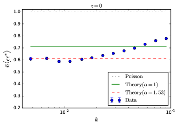
(a)

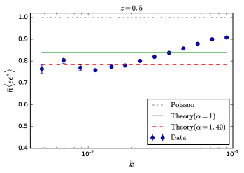
(b)

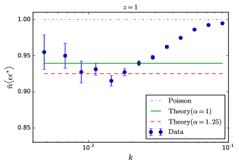
(c)

Figure 1: Noise power spectrum $P_{\epsilon\epsilon}(k)$ normalized to the Poisson expectation $1/\bar{n}$ as a function of wavenumber Results are shown for three different catalogues of massive halos, $M\gtrsim 10^{14}\ {\rm M_{\odot}/{\it h}}$, spanning the redshift range $0<z<1$. The dotted-dashed (grey) indicates the Poisson expectation, while the solid (green) and dashed (red) lines represent the halo model prediction $P_{\epsilon_{0}\epsilon_{0}}^{\{0\}}$ (see Eq.(64) with $\alpha=1$ and $\alpha$ fitted to the low-$k$ data points, respectively.

In order to test our algorithm, we generated 512 realizations of randomly distributed particles with the same number density as that of the halos extracted from the simulations. To compute the Fourier modes, we extrapolated these random distributions onto a regular cubical grid using the cloud-in-cell (CiC) assignment which, upon Fourier transformation, was corrected for with the appropriate window function. The resulting cumulative bispectrum was consistent with $1/\bar{n}^{2}$ within the error bars. A comparison of the cumulative matter bispectrum with the tree-level expression Eq.(3) induced by gravitational mode-coupling provided a second consistency check. We found a very good agreement between the simulated and theoretical $B_{\delta\delta\delta}(<k_{\text{max}})$, with a systematic deviation towards $k_{\text{max}}\sim 0.1\ {\rm{\it h}Mpc^{-1}}$ presumably consistent with the gradual rise of 1-loop contributions to the matter bispectrum.

Hereafter, we will discuss results obtained for the noise power spectrum, and the following cumulative bispectrum of halo noise and matter fluctuation fields:

$$B_{\epsilon\epsilon\epsilon}(<k_{\text{max}})=\frac{V^{2}}{N_{t}}\sum\epsilon(\textbf{\em k}_{1})\epsilon(\textbf{\em k}_{2})\epsilon^{*}(\textbf{\em k}_{1}+\textbf{\em k}_{2})$$

$$B_{\epsilon\epsilon\delta}(<k_{\text{max}})=\frac{V^{2}}{N_{t}}\sum\epsilon(\textbf{\em k}_{1})\epsilon(\textbf{\em k}_{2})\delta^{*}(\textbf{\em k}_{1}+\textbf{\em k}_{2})\;,$$ (63)

where the sum runs, again, over all pairs $\{\textbf{\em k}_{1},\textbf{\em k}_{2}\}$ such that ${0<k_{1},k_{2},|\textbf{\em k}_{1}+\textbf{\em k}_{2}|<k_{\text{max}}}$. The halo noise $\epsilon(\textbf{\em k})$ is defined as in Eq.(4), $\epsilon(\textbf{\em k})=\delta_{h}(\textbf{\em k})-b_{1}\delta(\textbf{\em k})$, where $b_{1}$ assumes the best-fit values listed in Table 1. Since it is pausible that the exclusion volume responsible for sub-Poissonian noise at large halo mass be different from $\overline{M}/\bar{\rho}_{m}$ (after all, halos do not have well defined boundaries, but rather a density profile which decays with the distance from the halo center), we multiply in Eqs.(14), (28) and (20) each factor of $M$ by a fudge factor $\alpha$. With this additional model parameter, our theoretical predictions based on Eqs.(34 and (36)) thus become:

$$P_{\epsilon_{0}\epsilon_{0}}^{\{0\}} =\frac{1}{\bar{n}}\bigg{\{}1-2\alpha b_{1}\left(\frac{\bar{n}\overline{M}}{\bar{\rho}_{m}}\right)+\alpha^{2}b_{1}^{2}\left(\frac{\bar{n}\langle nM^{2}\rangle}{\bar{\rho}_{m}^{2}}\right)\bigg{\}}$$

$$P_{\epsilon_{0}\epsilon_{\delta}}^{\{0\}} =\frac{b_{1}}{2\bar{n}}\bigg{\{}1-2\alpha\left(\frac{\bar{n}\overline{Mb_{1}}}{\bar{\rho}_{m}}\right)+\alpha^{2}b_{1}\left(\frac{\bar{n}\langle nM^{2}b_{1}\rangle}{\bar{\rho}_{m}^{2}}\right)\bigg{\}}$$

$$B_{\epsilon_{0}\epsilon_{0}\epsilon_{0}}^{\{0\}} =\frac{1}{\bar{n}^{2}}\bigg{\{}1-3\alpha b_{1}\left(\frac{\bar{n}\overline{M}}{\bar{\rho}_{m}}\right)+3\alpha^{2}b_{1}^{2}\left(\frac{\bar{n}^{2}\overline{M^{2}}}{\bar{\rho}_{m}^{2}}\right)$$

$$\qquad-\alpha^{3}b_{1}^{3}\left(\frac{\bar{n}^{2}\langle nM^{3}\rangle}{\bar{\rho}_{m}^{3}}\right)\bigg{\}}\;.$$ (64)

Note that, while $P_{\epsilon_{0}\epsilon_{0}}^{\{0\}}$ is nothing but the formula derived in Hamaus et al. (2010), the other expressions are new. To evaluate the average $\langle nM^{k}b_{1}^{l}\rangle$, we take the lower boundary of the integral to be equal to the mass of one dark matter particle, i.e. $1.2\times 10^{12}\ {\rm M_{\odot}/{\it h}}$. We use the Sheth-Tormen mass function and bias for this numerical evaluation Sheth & Tormen (1999), which matches the measured halo number densities to better than 10 percents at all redshifts. We have found that $\langle nM^{k}b_{1}^{l}\rangle$ does not change noticeably if we decrease further the lower bound of the integral. Furthermore, we assume $\overline{Mb_{1}}\approx\overline{M}b_{1}$ to rely as much as possible on the measured mass, number density and bias for the halo bin. The Sheth-Tormen mass function and bias suggest that $\overline{M}b_{1}$ underestimates the actual average $\overline{Mb_{1}}$ by $\sim 15$% (resp. $\sim$5 %) at $z=0$ (resp. $z=1$).

(a)

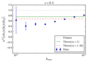
(b)

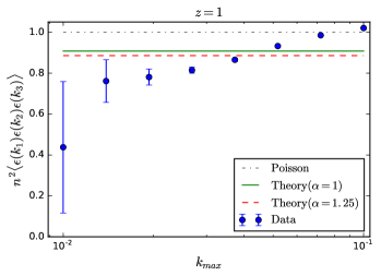
(c)

Figure 2: Measurements of the cummulative halo noise bispectrum $B_{\epsilon\epsilon\epsilon}(<k_{\text{max}})$ normalized to the Poisson expectation $1/\bar{n}^{2}$ as a function of the maximum wavenumber $k_{\text{max}}$. Results are shown at redshift $z=0$, 0.5 and 1. Error bars indicate the error on the mean as estimated from the full suite of simulations. The solid (green) lines is the halo model prediction with $\alpha=1$, whereas the dashed (red) line follows from setting $\alpha$ to its best-fit value inferred from the measurements of the halo noise power spectrum.

VI.3 Results

We first calculate the noise power spectrum $P_{\epsilon\epsilon}(k)$ and find that it lies significantly below the Poisson expectation $1/\bar{n}$, in agreement with the findings of Hamaus et al. (2010). This is summarized in Fig.1. The error bars represent the standard deviation of the mean, which is calculated from 512 realizations. The solid (green) curve indicates $P_{\epsilon_{0}\epsilon_{0}}^{\{0\}}$ for the fiducial value of $\alpha=1$, whereas the dashed (red) curve is a fit to the low-$k$ plateau seen in the figure (For $z=1$, we discarded the two data points with lowest wavenumbers). The best-fit values of $\alpha$ are quoted in the insert window. We will use the same values of $\alpha$ in subsequent comparison in order to assess the extent to which a single value of $\alpha=\alpha(M)$ can reproduce all the measurements. Furthermore, $P_{\epsilon\epsilon}(k)$ exhibits a strong scale-dependence for $k\gtrsim 0.2\ {\rm{\it h}Mpc^{-1}}$ similar to that seen in Biagetti et al. (2017). If the $k$-dependence of the noise power spectrum directly reflects that of the halo profile $u(k|M)$, as in Eq.(37) for instance, then it cannot explain the scale-dependence seen in Fig.1 because $u(k|M)$ remains very close to unity for $k\lesssim 0.1\ {\rm{\it h}Mpc^{-1}}$, even for massive halos. Clearly, the observed scale-dependence must therefore originate from the second- and higher- order terms in the definition of the halo shot noise, Eq.(4).

We now turn to the measurements of the cumulative halo noise bispectrum $B_{\epsilon\epsilon\epsilon}(<k_{\text{max}})$. They are shown in Fig.2 as a function of the maximum wavenumber $k_{\text{max}}$. Here again, the data lies consistently below the Poisson expectation $1/\bar{n}^{2}$. Unfortunately, the lowest data point is fairly noisy, so that it is difficult to identify any plateau which could unambigously help us determine the actual magnitude of $B_{\epsilon_{0}\epsilon_{0}\epsilon_{0}}^{\{0\}}$. The scale-dependence, which is more pronounced than in $P_{\epsilon\epsilon}(k)$, complicates this further. Moreover, using the best-fit value of $\alpha$ inferred from the measurements of $P_{\epsilon\epsilon}(k)$ only mildly improve the agreement at low wavenumber. At $z=0$ for instance, matching the data would require $\alpha\approx 2$.

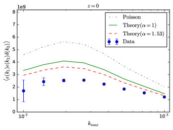
(a)

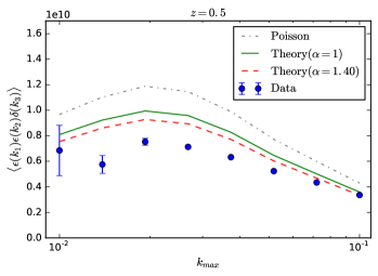
(b)

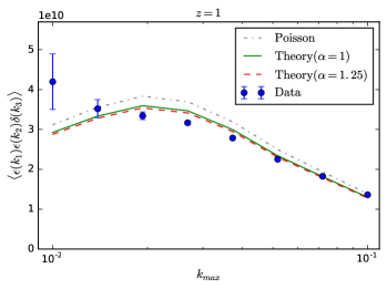
(c)

Figure 3: Same as Fig.2, but for the cummulative cross halo noise - matter bispectrum $B_{\epsilon\epsilon\delta}(<k_{\text{max}})$.

Finally, Fig.3 displays the measurements of the cumulative cross halo noise matter bispectrum $B_{\epsilon\epsilon\delta}(<k_{\text{max}})$ which, in the limit of small wavenumber, is given by

$$B_{\epsilon\epsilon\delta}(k_{1},k_{2},|\textbf{\em k}_{1}+\textbf{\em k}_{2}|)=2P_{\epsilon_{0}\epsilon_{\delta}}^{\{0\}}P_{\text{lin}}(|\textbf{\em k}_{1}+\textbf{\em k}_{2}|)\;.$$ (65)

This relation is Eq.(25) with $i=j$ and $B_{\epsilon_{0}\epsilon_{0}\delta}^{\{0\}}\equiv 0$, as predicted by our new halo model prescription. Here, $\textbf{\em k}_{1}+\textbf{\em k}_{2}$ is the wavevector carried by $\delta$. To produce a theoretical prediction for this statistics, we compute the cumulative power spectrum directly from the data, i.e. we estimate

$$P_{\text{lin}}(<k_{\text{max}})=\frac{V}{N_{t}}\sum\big{|}\delta(\textbf{\em k}_{1}+\textbf{\em k}_{2})\big{|}^{2}$$ (66)

where the sum over the pair $\{\textbf{\em k}_{1},\textbf{\em k}_{2}\}$ is subject to the same aforementioned conditions. For the amplitude of $P_{\epsilon_{0}\epsilon_{\delta}}^{\{0\}}$, we consider three estimates: the Poisson expectation $P_{\epsilon_{0}\epsilon_{\delta}}^{\{0\}}=b_{1}/2\bar{n}$, and the halo model prediction Eq.(64) with $\alpha=1$ and $\alpha$ fitted to the noise power spectrum. Overall, the data points consistently trace the shape of the matter power spectrum, in agreement with Eq.(65). Based on our data only however, we cannot exclude a non-zero value of $B_{\epsilon_{0}\epsilon_{0}\delta}^{\{0\}}$ at the level predicted by the “original” halo model, i.e. $B_{\epsilon_{0}\epsilon_{0}\delta}^{\{0\}}\sim\overline{M}/(\bar{n}\bar{\rho}_{m})\sim 10^{8-9}$ for the halos considered here. However, as we argued earlier, only $B_{\epsilon_{0}\epsilon_{0}\delta}^{\{0\}}\equiv 0$ or, equivalently, $\Xi_{ij\delta}\equiv 0$ is consistent with the halo shot noise being uncorrelated with the density.

Here again, the Poisson expectation overestimates the measurements. Our halo model prediction with best-fit $\alpha$ improves the agreement noticeably, but the match is not perfect. Therefore, the difference between our theoretical predictions and the data certainly cannot be captured with a single parameter $\alpha$. Nevertheless, the agreement between the various measurements and theoretical predictions is encouraging, and suggests that it should be possible to understand the shot noise of biased tracers using the halo model prescription advocated in this paper.

VII Discussion

VII.1 Optimal weights

Ref.Hamaus et al. (2010) showed that mass weighting reduces the noise of a halo catalogue and returns a weighted halo field whose correlation with the matter distribution is tighter. This is a consequence of the shot noise 2-point covariance having a zero eigenvalue, with corresponding eigenvector proportional to the halo mass Schmidt (2016). Here, we present yet another simple derivation of these results. We emphasize that the optimal weight is generally proportional to $M\,n(M)$ unless the halo mass bins are constructed to have identical number density (as is done in Hamaus et al. (2010); Hamaus, Seljak & Desjacques (2011)). We also point out that mass-weighting not only minimizes the white noise in the weighted power spectrum, but also cancel out the weighted bispectrum in the limit where all halos are resolved.

Let us split the halo distribution into mass bins and assign a weight $\lambda_{i}$ to each of them. For $k\ll 1$, the power spectrum of the weighted halo field is given by

$$P_{\lambda\lambda}(k) \equiv\sum_{i,j}\lambda_{i}\lambda_{j}\left(b_{i}b_{j}P_{\text{lin}}(k)+\frac{1}{\bar{n}_{i}}\delta_{ij}^{K}-b_{i}\frac{\overline{M_{j}}}{\bar{\rho}_{m}}-b_{j}\frac{\overline{M_{i}}}{\bar{\rho}_{m}}+b_{i}b_{j}\frac{\langle nM^{2}\rangle}{\bar{\rho}_{m}^{2}}\right)$$ (67)

$$=\sum_{i,j}\lambda_{i}\lambda_{j}b_{i}b_{j}P_{\text{lin}}(k)+\sum_{i,j}\lambda_{i}\lambda_{j}\left(\frac{1}{\bar{n}_{i}}\delta_{ij}^{K}-b_{i}\frac{\overline{M_{j}}}{\bar{\rho}_{m}}-b_{j}\frac{\overline{M_{i}}}{\bar{\rho}_{m}}+b_{i}b_{j}\frac{\langle nM^{2}\rangle}{\bar{\rho}_{m}^{2}}\right)\;.$$

Upon taking the continuous limit, $\overline{M_{i}}$ can be replaced by $M_{i}$, $\bar{n}_{i}$ by the halo mass function $n$ etc. We shall determine the weights $\lambda_{i}$ such that the power spectrum of our weighted halo field returns an unbiased estimate of the matter power spectrum. This leads the following two constraints:

$$\int\!dM\,\lambda(M)\,b_{1}(M)=1$$ (68)

and

$$\int \!dM\,\frac{\lambda^{2}(M)}{n(M)}+\int\!dM\int\!dM^{\prime}\,\lambda(M)\lambda(M^{\prime})$$

$$\times\left(-b_{1}(M)\frac{M^{\prime}}{\bar{\rho}_{m}}-b_{1}(M^{\prime})\frac{M}{\bar{\rho}_{m}}+b_{1}(M)b_{1}(M^{\prime})\frac{\langle nM^{2}\rangle}{\bar{\rho}_{m}^{2}}\right)$$

$$=0\;.$$ (69)

To determine $\lambda(M)$, we rely on the peak-background split relation Eq.(23) for the linear halo bias and the halo model assumpation that all the mass is in halos, that is,

$$\int\!dM\,M\,n(M)=\bar{\rho}_{m}\;.$$ (70)

This implies

$$\frac{\partial}{\partial\bar{\rho}_{m}}\int\!dM\,M\,n(M) =\int\!dM\,M\frac{\partial n}{\partial\bar{\rho}_{m}}$$

$$=\int\!dM\,\left(M\frac{n}{\bar{\rho}_{m}}\right)\frac{\bar{\rho}_{m}}{n}\frac{\partial n}{\partial\bar{\rho}_{m}}$$

$$=1\;.$$ (71)

Comparing the last equality with Eq.(68) and taking advantage of Eq.(23), the desired weight is

$$\lambda(M)=\frac{n(M)M}{\bar{\rho}_{m}}\;.$$ (72)

In contrast to Hamaus et al. (2010); Hamaus, Seljak & Desjacques (2011), there is an additional multiplicative factor of $n(M)$ because we do not enforce the mass bins to have the same number density. Nevertheless, there is no contradiction with their findings since they either considered finite mass bins with identical number density or directly weighted the halo density $n_{h}(\textbf{\em x})=\bar{n}\delta_{h}(\textbf{\em x})$, in which case the factor of $\bar{n}$ was implicitly accounted for. Substituting this solution into the second condition Eq.(69) yields

$$\int\!dM\,\frac{1}{n}\left(M\frac{n}{\bar{\rho}_{m}}\right)^{2}-\frac{2}{\bar{\rho}_{m}} \int\!dM\,M\frac{n}{\bar{\rho}_{m}}\left(\frac{\bar{\rho}_{m}}{n}\frac{\partial n}{\partial\bar{\rho}_{m}}\right)\int\!dM^{\prime}\,M^{\prime}\left(M^{\prime}\frac{n}{\bar{\rho}_{m}}\right)+\frac{\langle nM^{2}\rangle}{\bar{\rho}_{m}^{2}}\left[\int\!dM\,M\frac{n}{\bar{\rho}_{m}}\left(\frac{\bar{\rho}_{m}}{n}\frac{\partial n}{\partial\bar{\rho}_{m}}\right)\right]^{2}$$

$$=\frac{\langle nM^{2}\rangle}{\bar{\rho}_{m}^{2}}-\frac{2}{\bar{\rho}_{m}^{2}}\int\!dM\,M\frac{\partial n}{\partial\bar{\rho}_{m}}\int\!dM^{\prime}\,n(M^{\prime})\,(M^{\prime})^{2}+\frac{\langle nM^{2}\rangle}{\bar{\rho}_{m}^{2}}$$

$$\equiv 0\;.$$ (73)

This demonstrates that the weight Eq.(72) also gives zero shot-noise in the limit where all halos down to $M=0$ are resolved. Therefore, weighting halos with $\bar{n}M/\bar{\rho}_{m}$ yields an unbiased estimate of the linear matter power spectrum with zero white noise, in agreement with the numerical experiment of Hamaus et al. (2010).

Our derivation can be easily extended to higher-order statistics. Namely, ignoring any primordial non-Gaussianity, the bispectrum of the weighted halo field on large scales can be read off from Eq.(2):

$$B_{\lambda\lambda\lambda}(k_{1},k_{2},k_{3}) \equiv\sum_{i,j,k}\lambda_{i}\lambda_{j}\lambda_{k}\bigg{\{}b_{1}^{(i)}b_{1}^{(j)}\bigg{[}b_{2}^{(k)}+2b_{K^{2}}^{(k)}\left(\mu_{23}^{2}-\frac{1}{3}\right)\bigg{]}P_{\text{lin}}(k_{2})P_{\text{lin}}(k_{3})+\mbox{(2 cyc.)}\bigg{\}}+\sum_{i,j,k}\lambda_{i}\lambda_{j}\lambda_{k}B_{\epsilon_{0i}\epsilon_{0j}\epsilon_{0k}}^{\{0\}}\;,$$ (74)

with the white noise contribution given by Eq.(19). We have labelled the halo mass bins with superscripts to improve the readability of this equation. Using the peak-background split relation

$$b_{N}=\frac{\bar{\rho}_{m}^{N}}{n}\frac{\partial^{N}n}{\partial\bar{\rho}_{m}^{N}}$$ (75)

for the LIMD bias parameters, the weighted average of $b_{N}$ reduces to

$$\int\!dM\,\lambda(M)\,b_{N}(M) =\bar{\rho}_{m}^{N-1}\frac{\partial^{N}}{\partial\bar{\rho}_{m}^{N}}\int\!dM\,M\,n(M)$$

$$=\delta_{N1}^{K}\;,$$ (76)

i.e. they vanish unless $N=1$. The weighted sum of the tidal shear bias $b_{K_{2}}$ also vanishes in the limit where all halos are resolved because the shear is uncorrelated with the average density $\bar{\rho}_{m}$. Furthermore, one can easily check that, in the same limit, the optimal weight Eq.(72) cancels out the white noise contribution to the weighted bispectrum:

$$\sum_{i,j,k}\lambda_{i} \lambda_{j}\lambda_{k}B_{\epsilon_{0i}\epsilon_{0j}\epsilon_{0k}}^{\{0\}}$$ (77)

$$=-\frac{\langle nM^{3}\rangle}{\bar{\rho}_{m}^{3}}+3\frac{\langle nM^{3}\rangle}{\bar{\rho}_{m}^{3}}-3\frac{\langle nM^{3}\rangle}{\bar{\rho}_{m}^{3}}+\frac{\langle nM^{3}\rangle}{\bar{\rho}_{m}^{3}}$$

$$\equiv 0\;.$$

Therefore, the mass-weighted halo bispectrum vanishes in the limit where the minimum halo mass resolved is $M_{\text{min}}=0$. In other words, mass-weighting returns the linear matter density field at tree-level in perturbation theory. We have not investigated whether this cancellation occurs at higher order.

VII.2 From halos to galaxies

Our approach can be readily extended to compute shot noise corrections to galaxy clustering statistics. Here, we outline how this can be done assuming, for simplicity, that galaxies follow Poisson statistics, that is, the subhalos hosting galaxies do not exclude each other (see, e.g., Cacciato et al. (2012) for a more realistic treatment). We defer a more detailed study to future work.

For illustrative purposes, we shall focus on the $k\to 0$ white noise correction to the galaxy power spectrum, which we also denote as $P_{\epsilon_{0}\epsilon_{0}}^{\{0\}}$. As a rule of thumb, the galaxy shot noise contributions can be obtained upon making the replacement

$$\frac{\Theta(M,M_{i})}{\bar{n}_{i}}\to\frac{N_{g}(M)}{\bar{n}_{g}}u_{g}(k|M)$$ (78)

in all halo model expressions. Here, $N_{g}$ is the number of galaxies in halos of mass $M$, whereas $u_{g}(k|M)$ is the Fourier transform of the average density profile of galaxies residing in halos of mass $M$ . The probability distribution $p(N_{g})$ of having exactly $N_{g}$ galaxies in a halo of mass $M$ characterizes as given halo occupation distribution (HOD) model (see, for instance,Zheng, Coil & Zehavi (2007); Abramo et al. (2015) and references therein).

In practice, galaxy populations are usually split into central and satellite galaxies, which have different colors and morphologies. By definition, there is only zero or one central galaxy per halo, i.e. $N_{c}=0$ or 1. This implies $\overline{N_{c}^{k}}=\overline{N_{c}}$. Furthermore, one usually assumes that the existence of satellite galaxies is conditioned on the presence of a central galaxy, ie. $N_{s}=N_{c}\mathcal{N}_{s}$. Since $P(N_{c},\mathcal{N}_{s}|M)\equiv P(N_{c}|M)P(\mathcal{N}_{s}|M)$, this implies $\overline{N_{c}^{k}\mathcal{N}_{s}^{l}}=\overline{N_{c}}\overline{\mathcal{N}_{s}^{l}}$. Therefore, the average number of galaxies per halo of mass $M$ is

$$\big{\langle}N_{g}\big{\lvert}M\big{\rangle}=\overline{N}_{c}(M)(1+\overline{\mathcal{N}_{s}}(M))\;,$$ (79)

so that the galaxy number density is given by

$$\bar{n}_{g}=\int\!dM\,n(M)\,\overline{N}_{c}(M)\big{[}1+\overline{\mathcal{N}_{s}}(M)\big{]}\;.$$ (80)

Analogously, the linear LIMD galaxy bias $b_{g}$ and the average host halo mass $\overline{M}_{g}$ are

$$b_{g}=\frac{1}{\bar{n}_{g}}\int\!dM\,n(M)b_{1}(M)\overline{N_{c}}(M)\big{[}1+\overline{\mathcal{N}_{s}}(M)\big{]}$$ (81)

and

$$\overline{M}_{g}\equiv\frac{1}{\bar{n}_{g}}\int\!dM\,Mn(M)\,\overline{N_{c}}(M)\big{[}1+\overline{\mathcal{N}_{s}}(M)\big{]}\;.$$ (82)

Note that $\overline{M}_{g}$ is strongly weighted towards high masses because of its dependence on the number $\mathcal{N}_{s}$ of satellite galaxies. Finally, if the number of satellites follows a Poisson distribution, then $\overline{\mathcal{N}_{s}^{2}}=\overline{\mathcal{N}_{s}}$ also holds. Note that, although the total galaxy density profile $u_{g}(k|M)$ is well approximated by the dark matter profile $u(k|M)$, the density profiles $u_{c}(k|M)$ and $u_{s}(k|M)$ of central and satellite galaxies are generally different because central galaxies tend to reside near the host halo center. Nevertheless, this distinction is irrelevant here as we are only interested in the low $k$ behaviour, in which all profiles asymptote to unity.

In analogy with halos, the white noise contribution to the galaxy power spectrum thus is given by

$$P_{\epsilon_{0}\epsilon_{0}}^{\{0\}}\stackrel{{\scriptstyle k\to 0}}{{=}}P_{gg}^{\text{1H}}(k)-2b_{g}P_{g\delta}^{\text{1H}}(k)+b_{g}^{2}P_{\delta\delta}^{\text{1H}}(k)\;.$$ (83)

The contribution from galaxy pairs sitting in the same halo gives the 1-halo term

$$P^{\text{1H}}_{gg}(k) \stackrel{{\scriptstyle k\to 0}}{{=}}\frac{1}{\bar{n}_{g}^{2}}\int\!dM\,n(M)\,\big{\langle}N_{g}\cdot N_{g}\big{\lvert}M\big{\rangle}$$ (84)

$$=\frac{1}{\bar{n}_{g}}+\frac{1}{\bar{n}_{g}^{2}}\int\!dM\,n(M)\big{\langle}N_{g}(N_{g}-1)\big{\lvert}M\big{\rangle}$$

$$=\frac{1}{\bar{n}_{g}}+\frac{1}{\bar{n}_{g}^{2}}\int\!dM\,n(M)\,\overline{N}_{c}(M)$$

$$\qquad\times\Big{[}2\overline{\mathcal{N}_{s}}(M)+\overline{\mathcal{N}_{s}}^{2}(M)\Big{]}\;.$$

The first term in the second and last equality of Eq.(84) is the usual Poisson noise (induced by self-pairs), whereas the second term in the contribution from pairs inside the same halo. There is not factor of $1/2$ because galaxy pairs are formally distinguishable. Similarly, the 1-halo galaxy - density contribution is

$$P^{\text{1H}}_{g\delta}(k) \stackrel{{\scriptstyle k\to 0}}{{=}}\frac{1}{\bar{\rho}_{m}\bar{n}_{g}}\int\!dM\,Mn(M)\,\big{\langle}N_{g}\big{\lvert}M\big{\rangle}$$

$$=\frac{1}{\bar{\rho}_{m}\bar{n}_{g}}\int\!dM\,Mn(M)\,\overline{N}_{c}(M)\big{[}1+\overline{\mathcal{N}_{s}}(M)\big{]}$$

$$=\frac{\overline{M}_{g}}{\bar{\rho}_{m}}\;.$$ (85)

Finally, the 1-halo matter power spectrum is unchanged and equal to $\langle nM^{2}\rangle/\bar{\rho}_{m}^{2}$ in the limit $k\to 0$. Therefore, the galaxy white noise is

$$P_{\epsilon_{0}\epsilon_{0}}^{\{0\}} =\frac{1}{\bar{n}_{g}}+\frac{1}{\bar{n}_{g}^{2}}\int\!dM\,n(M)\,\overline{N}_{c}\Big{(}2\overline{\mathcal{N}_{s}}+\overline{\mathcal{N}_{s}}^{2}\Big{)}$$

$$\qquad-2b_{g}\frac{\overline{M}_{g}}{\bar{\rho}_{m}}+b_{g}^{2}\frac{\langle nM^{2}\rangle}{\bar{\rho}_{m}^{2}}\;.$$ (86)

The second line in the right-hand side is the non-Poissonian correction. With our approximations, only the first moment $\overline{N_{c}}$ and $\overline{\mathcal{N}_{s}}$ need to be specified in order to predict the white noise contribution to the galaxy power spectrum.

VIII Conclusions

Understanding the shot noise of biased tracers beyond the simple Poissonian approximation becomes increasingly relevant as the statistical uncertainties are expected to decrease significantly in forthcoming galaxy redshift surveys. In this work, we have shown how the halo model to large scale structure, which has been widely applied and studied, can be used to provide meaningful predictions for the shot noise contributions to halo clustering statistics. In essence, the various sources of shot noise in the halo model must be rearranged such that they are all absorbed in the halo fluctuation field. The resulting perturbative expansion can be mapped onto the general bias expansion, so that the various (renormalized) shot noise terms can be clearly expressed as combinations of the halo model shot noises. In combination with halo occupation distributions, our approach can furnish useful quantitative estimates for the shot noise contributions to galaxy clustering (which remain thus far poorly constrained).

Furthermore, we have demonstrated how the constant white noise contributions are connected to volume integrals over halo correlation functions and their response to a long-wavelength density perturbation. These relations define a new class of consistency relations for discrete large scale structure tracers. Interestingly, our revised halo model precisely reproduces these consistency relations. Note that these volume integrals could also be computed using fully nonlinear description of halo clustering, such as peak theory for instance (as in, e.g., Baldauf et al. (2013, 2016)). However, our halo model prescription has the advantage of being far more flexible as it does not require any sophisticated numerical evaluations.

Finally, we have also presented a comparison of our theoretical predictions with measurements of halo shot noise bispectra extracted from a large suite of numerical simulations. We have found that, for the massive halos considered here, the various bispectrum shot noise statistics are significantly sub-Poissonian, in agreement with Casas-Miranda et al. (2002); Seljak, Hamaus & Desjacques (2009) and the more recent power spectrum analysis of Hamaus et al. (2010). Our halo model -based predictions fare reasonably well, yet the match is not perfect. Among the possible sources of discrepancy is the fact that we have assumed a unique, perfectly symmetric halo profile while density profiles certainly vary in shape on a halo-by-halo basis. Moreover, our assumption $\langle\epsilon\delta\rangle=0$ etc. implies that the halo profile (which creates the exclusion volume responsible for sub-Poissonian noise at large halo mass) is uncorrelated with density fluctuations. This may not hold at all order if halo profiles retain memory of the initial conditions or the halo assembly history.

Thus far, our halo model prescription is, arguably, more an educated guess than a rigorous theoretical construction, but we believe it can furnish useful insights towards a comprehensive description of the clustering of discrete large scale structure tracers.

Appendix A A collection of halo model formulae

We give explicit expressions for the 1-halo, 2-halo and 3-halo contributions to cross halo-matter power spectra and bispectra without restriction on the wavenumbers. We adopt the notation of Smith, Scoccimarro & Sheth (2007); Hamaus et al. (2010): each halo fluctuation field brings a factor of $\Theta(M,M_{i})/\bar{n}_{i}$, whereas each matter fluctuation fields carries a factor of $(M/\bar{\rho}_{m})u(k|M)$. While there is no factor of $u(k|M)$ for halos (since, by definition, halo centers lie at the center of the average halo profile), matter fluctuation field carry a factor of $u(k|M)$. The 1-halo power spectra are given by

$$P^{\text{1H}}_{ij}(k) =\frac{1}{\bar{n}_{i}\bar{n}_{j}}\int\!dM\,n(M)\Theta(M,M_{i})\Theta(M,M_{j})$$

$$P^{\text{1H}}_{i\delta}(k) =\frac{1}{\bar{n}_{i}\bar{\rho}_{m}}\int\!dM\,Mn(M)\Theta(M,M_{i})u(k|M)$$

$$P^{\text{1H}}_{\delta\delta}(k) =\frac{1}{\bar{\rho}_{m}^{2}}\int\!dM\,M^{2}n(M)u(k|M)^{2}\;,$$ (87)

where the Fourier transform $u(k|M)$ of the halo profile asymptotes to unity in the large scale limit $k\to 0$. Analogously, the 1-halo bispectra are given by

$$B^{\text{1H}}_{ijk}(k_{1},k_{2},k_{3}) =\frac{1}{\bar{n}_{i}\bar{n}_{j}\bar{n}_{k}}\int\!dM\,n(M)\Theta(M,M_{i})\Theta(M,M_{j})$$

$$\qquad\times\Theta(M,M_{k})$$

$$B^{\text{1H}}_{ij\delta}(k_{1},k_{2},k_{3}) =\frac{1}{\bar{n}_{i}\bar{n}_{j}\bar{\rho}_{m}}\int\!dM\,Mn(M)\Theta(M,M_{i})$$

$$\qquad\times\Theta(M,M_{j})u(k_{3}|M)$$

$$B^{\text{1H}}_{i\delta\delta}(k_{1},k_{2},k_{3}) =\frac{1}{\bar{n}_{i}\bar{\rho}_{m}^{2}}\int\!dM\,M^{2}n(M)\Theta(M,M_{i})$$

$$\qquad\times\prod_{\alpha=2}^{3}u(k_{\alpha}|M)$$

$$B^{\text{1H}}_{\delta\delta\delta}(k_{1},k_{2},k_{3}) =\frac{1}{\bar{\rho}_{m}^{3}}\int\!dM\,M^{3}n(M)\prod_{\alpha=1}^{3}u(k_{\alpha}|M)\;.$$ (88)

Finally, the 2-halo contribution to the bispectra are

$$B^{\text{2H}}_{ij\delta}(k_{1},k_{2},k_{3}) =\frac{1}{\bar{n}_{i}\bar{n}_{j}\bar{\rho}_{m}}\int\!dM\,\Theta(M,M_{i})n(M)b_{1}(M)\int\!dM^{\prime}\,\Theta(M^{\prime},M_{j})M^{\prime}n(M^{\prime})b_{1}(M^{\prime})u(k_{3}|M^{\prime})P_{\text{lin}}(k_{1})$$ (89)

$$\quad+\frac{1}{\bar{n}_{i}\bar{n}_{j}\bar{\rho}_{m}}\int\!dM\,\Theta(M,M_{j})n(M)b_{1}(M)\int\!dM^{\prime}\,\Theta(M^{\prime},M_{i})M^{\prime}n(M^{\prime})b_{1}(M^{\prime})u(k_{3}|M^{\prime})P_{\text{lin}}(k_{2})$$

$$\quad+\frac{1}{\bar{n}_{i}\bar{n}_{j}\bar{\rho}_{m}}\int\!dM\,Mn(M)b_{1}(M)u(k_{3}|M)\int\!dM^{\prime}\,\Theta(M^{\prime},M_{i})\Theta(M^{\prime},M_{j})n(M^{\prime})b_{1}(M^{\prime})P_{\text{lin}}(k_{3})$$

$$B^{\text{2H}}_{i\delta\delta}(k_{1},k_{2},k_{3}) =\frac{1}{\bar{n}_{i}\bar{\rho}_{m}^{2}}\int\!dM\,\Theta(M,M_{i})n(M)b_{1}(M)\int\!dM^{\prime}\,(M^{\prime})^{2}n(M^{\prime})b_{1}(M^{\prime})u(k_{2}|M)u(k_{3}|M)P_{\text{lin}}(k_{1})$$

$$\quad+\bigg{\{}\frac{1}{\bar{n}_{i}\bar{\rho}_{m}^{2}}\int\!dM\,Mn(M)b_{1}(M)u(k_{2}|M)\int\!dM^{\prime}\,\Theta(M^{\prime},M_{i})M^{\prime}n(M^{\prime})b_{1}(M^{\prime})u(k_{3}|M^{\prime})P_{\text{lin}}(k_{2})+2\leftrightarrow 3\bigg{\}}$$

$$B^{\text{2H}}_{\delta\delta\delta}(k_{1},k_{2},k_{3}) =\frac{1}{\bar{\rho}_{m}^{3}}\int\!dM\,Mn(M)b_{1}(M)u(k_{3}|M)\int\!dM^{\prime}\,\big{(}M^{\prime}\big{)}^{2}n(M^{\prime})b_{1}(M^{\prime})u(k_{1}|M^{\prime})u(k_{2}|M^{\prime})P_{\text{lin}}(k_{3})+\mbox{(2 cyc.)}$$

Notice the factor of $b_{1}(M)b_{1}(M^{\prime})$, which follows from expanding the power spectrum of halo centers at linear order. In the limit $k_{i}\to 0$, these relations yield Eqs.(8), (18) and (21) of the main text.

Appendix B The halo shot noise trispectrum

To illustrate the applicability of the halo model approach beyond the bispectrum, we compute the Poissonian and non-Poissonian contributions to the constant white noise in the trispectrum of the halo shot noise $\epsilon_{i}(\textbf{\em k})$ (defined in Eq.(4)). We show that this result furnishes an estimate for the volume integral of the halo 4-point function.

Following our definition of the bispectrum, the trispectrum of 4 fluctuation fields reads $T_{WXYZ}(k_{1},k_{2},k_{3},k_{4})\equiv\langle W(\textbf{\em k}_{1})X(\textbf{\em k}_{2})Y(\textbf{\em k}_{3})Z(\textbf{\em k}_{4})\rangle_{c}^{\prime}$. Here, the prime signifies that we have removed a factor of $(2\pi)^{3}\delta^{D}\!(\textbf{\em k}_{1}+\textbf{\em k}_{2}+\textbf{\em k}_{3}+\textbf{\em k}_{4})$ owing to the invariance under translations; whereas the subscript “c” signifies that we should extract the connected piece. To compute the halo noise trispectrum $T_{\epsilon_{i}\epsilon_{j}\epsilon_{k}\epsilon_{l}}(k_{1},k_{2},k_{3},k_{4})\equiv\langle\epsilon_{i}(\textbf{\em k}_{1})\epsilon_{j}(\textbf{\em k}_{2})\epsilon_{k}(\textbf{\em k}_{3})\epsilon_{l}(\textbf{\em k}_{4})\rangle_{c}^{\prime}$, we start from the configuration space correlation of four halo noise fields:

$$\big{\langle}\epsilon_{i}\epsilon_{j}\epsilon_{k} \epsilon_{l}\big{\rangle}=\Big{\langle}\big{(}\delta_{i}-b_{i}\delta\big{)}\big{(}\delta_{j}-b_{j}\delta\big{)}\big{(}\delta_{k}-b_{k}\delta\big{)}\big{(}\delta_{l}-b_{l}\delta\big{)}\Big{\rangle}$$ (90)

$$=\langle\delta_{i}\delta_{j}\delta_{k}\delta_{l}\rangle-\Big{[}b_{l}\langle\delta_{i}\delta_{j}\delta_{k}\delta\rangle+\mbox{(3 cyc.)}\Big{]}+\Big{[}b_{k}b_{l}\langle\delta_{i}\delta_{j}\delta^{2}\rangle+\mbox{(5 perms.)}\Big{]}-\Big{[}b_{j}b_{k}b_{l}\langle\delta_{i}\delta^{3}\rangle+\mbox{(3 cyc.)}\Big{]}$$

$$\qquad+b_{i}b_{j}b_{k}b_{l}\langle\delta^{4}\rangle\;,$$

where it is understood that they are evaluated at position $\textbf{\em x}_{1}$, … , $\textbf{\em x}_{4}$. Substituting the definition of the halo fluctuation field Eq.(9), the calculation of the halo-matter 4-point functions is immediate (see Chan & Blot (2016) for instance). After some algebra, we obtain:

$$\Big{\langle}\delta_{i}(\textbf{\em x}_{1})\delta_{j}(\textbf{\em x}_{2})\delta_{k}(\textbf{\em x}_{3})\delta_{l}(\textbf{\em x}_{4})\Big{\rangle} =\xi_{ijkl}(\textbf{\em r}_{12},\textbf{\em r}_{13},\textbf{\em r}_{14})+\bigg{[}\frac{\delta_{ij}^{K}}{\bar{n}_{i}}\delta^{D}\!(\textbf{\em r}_{12})\Big{(}\xi_{kl}(\textbf{\em r}_{34})+\xi_{jkl}(\textbf{\em r}_{23},\textbf{\em r}_{34})\Big{)}+\mbox{(5 perms.)}\bigg{]}$$

$$\qquad+\bigg{[}\frac{\delta_{ij}^{K}}{\bar{n}_{i}}\frac{\delta_{kl}^{K}}{\bar{n}_{k}}\delta^{D}\!(\textbf{\em r}_{12})\delta^{D}\!(\textbf{\em r}_{34})\Big{(}1+\xi_{ik}(\textbf{\em r}_{13})\Big{)}+\mbox{(2 cyc.)}\bigg{]}$$

$$\qquad+\bigg{[}\frac{\delta_{ijk}^{K}}{\bar{n}_{i}^{2}}\delta^{D}\!(\textbf{\em r}_{13})\delta^{D}\!(\textbf{\em r}_{13})\xi_{kl}(\textbf{\em r}_{34})+\mbox{(3 cyc.)}\bigg{]}+\frac{\delta^{K}_{ijkl}}{\bar{n}_{i}^{3}}\delta^{D}\!(\textbf{\em r}_{14})\delta^{D}\!(\textbf{\em r}_{13})\delta^{D}\!(\textbf{\em r}_{12})$$

$$\Big{\langle}\delta_{i}(\textbf{\em x}_{1})\delta_{j}(\textbf{\em x}_{2})\delta_{k}(\textbf{\em x}_{3})\delta(\textbf{\em x}_{4})\Big{\rangle} =\xi_{ijk\delta}(\textbf{\em r}_{12},\textbf{\em r}_{13},\textbf{\em r}_{14})+\bigg{[}\frac{\delta_{ij}^{K}}{\bar{n}_{i}}\delta^{D}\!(\textbf{\em r}_{12})\xi_{ik\delta}(\textbf{\em r}_{13},\textbf{\em r}_{14})+\mbox{(2 cyc.)}\bigg{]}+\frac{\delta^{K}_{ijk}}{\bar{n}_{i}^{2}}\delta^{D}\!(\textbf{\em r}_{12})\delta^{D}\!(\textbf{\em r}_{13})\xi_{i\delta}(\textbf{\em r}_{14})$$

$$\Big{\langle}\delta_{i}(\textbf{\em x}_{1})\delta_{j}(\textbf{\em x}_{2})\delta(\textbf{\em x}_{3})\delta(\textbf{\em x}_{4})\Big{\rangle} =\xi_{ij\delta\delta}(\textbf{\em r}_{12},\textbf{\em r}_{13},\textbf{\em r}_{14})+\frac{\delta_{ij}^{K}}{\bar{n}_{i}}\delta^{D}\!(\textbf{\em r}_{12})\xi_{i\delta\delta}(\textbf{\em r}_{13},\textbf{\em r}_{14})\;.$$ (91)

Upon Fourier transforming the result and taking the large scale limit $k_{i}\to 0$, the Fourier space correlator of four halo fluctuation fields reads

$$\Big{\langle}\delta_{i}(\textbf{\em k}_{1})\delta_{j}(\textbf{\em k}_{2})\delta_{k}(\textbf{\em k}_{3})\delta_{l}(\textbf{\em k}_{4})\Big{\rangle}^{\prime} \stackrel{{\scriptstyle k_{i}\to 0}}{{=}}\Xi_{ijkl}+\bigg{[}\frac{\delta_{ij}^{K}}{\bar{n}_{i}}\Big{(}\delta^{D}\!(\textbf{\em k}_{1}+\textbf{\em k}_{2})\Xi_{kl}+\Xi_{jkl}\Big{)}+\mbox{(5 perms.)}\bigg{]}$$

$$\qquad+\bigg{[}\frac{\delta_{ij}^{K}}{\bar{n}_{i}}\frac{\delta_{kl}^{K}}{\bar{n}_{k}}\Big{(}\delta^{D}\!(\textbf{\em k}_{1}+\textbf{\em k}_{2})+\Xi_{ik}\Big{)}+\mbox{(2 cyc.)}\bigg{]}+\bigg{[}\frac{\delta_{ijk}^{K}}{\bar{n}_{i}^{2}}\Xi_{kl}+\mbox{(3 cyc.)}\bigg{]}+\frac{\delta_{ijkl}^{K}}{\bar{n}_{i}^{3}}\;.$$ (92)

Note that we have omitted a factor of $\delta^{D}\!(\textbf{\em k}_{3}+\textbf{\em k}_{4})$ in the second line, which is trivially implied by invariance under translations. Analogously, we find

$$\Big{\langle}\delta_{i}(\textbf{\em k}_{1})\delta_{j}(\textbf{\em k}_{2})\delta_{k}(\textbf{\em k}_{3})\delta(\textbf{\em k}_{4})\Big{\rangle}^{\prime} \stackrel{{\scriptstyle k_{i}\to 0}}{{=}}\Xi_{ijk\delta}+\frac{\delta_{ij}^{K}}{\bar{n}_{i}}\Xi_{i\delta\delta}\equiv 0$$

$$\Big{\langle}\delta_{i}(\textbf{\em k}_{1})\delta_{j}(\textbf{\em k}_{2})\delta(\textbf{\em k}_{3})\delta(\textbf{\em k}_{4})\Big{\rangle}^{\prime} \stackrel{{\scriptstyle k_{i}\to 0}}{{=}}\Xi_{ij\delta\delta}\equiv 0$$ (93)

for the 4-point cross-covariances since $\Xi$ vanishes as soon as there is at least one density field. Putting these results together, and taking advantage of the fact that the connected piece in Eq.(92) corresponds to the terms without a Dirac distribution Matarrese, Verde & Heavens (1997), the white noise contribution $T_{\epsilon_{i}\epsilon_{j}\epsilon_{k}\epsilon_{l}}(k_{i}\to 0)\equiv T_{\epsilon_{0i}\epsilon_{0j}\epsilon_{0k}\epsilon_{0l}}^{\{0\}}$ to the halo shot noise trispectrum eventually reads

$$T_{\epsilon_{0i}\epsilon_{0j}\epsilon_{0k}\epsilon_{0l}}^{\{0\}} =\Xi_{ijkl}+\bigg{[}\frac{\delta_{ij}^{K}}{\bar{n}_{i}}\Xi_{jkl}+\mbox{(5 perms.)}\bigg{]}$$ (94)

$$\quad+\bigg{[}\frac{\delta_{ij}^{K}}{\bar{n}_{i}}\frac{\delta_{kl}^{K}}{\bar{n}_{k}}\Xi_{ik}+\mbox{(2 cyc.)}\bigg{]}$$

$$\quad+\bigg{[}\frac{\delta_{ijk}^{K}}{\bar{n}_{i}^{2}}\Xi_{kl}+\mbox{(3 cyc.)}\bigg{]}+\frac{\delta_{ijkl}^{K}}{\bar{n}_{i}^{3}}\;.$$

This should be compared to the prediction obtained from our halo model ansatz Eqs.(34) and (36). The contribution arises from the correlators of the halo shot noise $\tilde{\epsilon}_{0i}$ and $\tilde{\epsilon}_{0m}$. Like $B_{\epsilon_{0}\epsilon_{0}\epsilon_{0}}^{\{0\}}$, they are given by the 1-halo trispectrum pieces of the “original” halo model since the 2-halo etc. terms involve factors of $P_{\text{lin}}(k)$ etc. We eventually obtain

$$T_{\epsilon_{0i}\epsilon_{0j}\epsilon_{0k}\epsilon_{0l}}^{\{0\}} =b_{i}b_{j}b_{k}b_{l}\frac{\langle nM^{4}\rangle}{\bar{\rho}_{m}^{4}}-\bigg{[}b_{i}b_{j}b_{k}\frac{\overline{M_{l}^{3}}}{\bar{\rho}_{m}^{3}}+\mbox{(3 cyc.)}\bigg{]}$$

$$\quad+\bigg{[}b_{i}b_{j}\frac{\overline{M_{k}^{2}}}{\bar{n}_{k}\bar{\rho}_{m}^{2}}\delta_{kl}^{K}+\mbox{(5 perms.)}\bigg{]}$$ (95)

$$\quad-\bigg{[}b_{i}\left(\frac{\overline{M_{j}}}{\bar{n}_{j}^{2}\bar{\rho}_{m}}\right)\delta_{jkl}^{K}+\mbox{(3 cyc.)}\bigg{]}+\frac{\delta_{ijkl}^{K}}{\bar{n}_{i}^{3}}\;.$$

On comparing Eqs. (94) and (95) and using the explicit expressions of $\Xi_{ij}$ and $\Xi_{ijk}$ given in Eqs.(43) and (49), the prediction for $\Xi_{ijkl}$ follows immediately.

References

• Abramo et al. (2015) Abramo L. R., Balmès I., Lacasa F., Lima M., 2015, Mon. Not. Roy. Astron. Soc., 454, 2844
• Baldauf et al. (2016) Baldauf T., Codis S., Desjacques V., Pichon C., 2016, Mon. Not. Roy. Astron. Soc., 456, 3985
• Baldauf et al. (2011) Baldauf T., Seljak U., Senatore L., Zaldarriaga M., 2011, JCAP, 1110, 031
• Baldauf et al. (2013) Baldauf T., Seljak U., Smith R. E., Hamaus N., Desjacques V., 2013, Phys. Rev., D88, 083507
• Biagetti et al. (2017) Biagetti M., Lazeyras T., Baldauf T., Desjacques V., Schmidt F., 2017, Mon. Not. Roy. Astron. Soc., 468, 3277
• Biagetti et al. (2013) Biagetti M., Perrier H., Riotto A., Desjacques V., 2013, Phys. Rev., D87, 063521
• Blot et al. (2015) Blot L., Corasaniti P. S., Alimi J.-M., Reverdy V., Rasera Y., 2015, Mon. Not. Roy. Astron. Soc., 446, 1756
• Cacciato et al. (2012) Cacciato M., Lahav O., Bosch F. C. v. d., Hoekstra H., Dekel A., 2012, Mon. Not. Roy. Astron. Soc., 426, 566
• Casas-Miranda et al. (2002) Casas-Miranda R., Mo H. J., Sheth R. K., Boerner G., 2002, Mon. Not. R. Astron. Soc., 333, 730
• Chan & Blot (2016) Chan K. C., Blot L., 2016
• Cooray & Sheth (2002) Cooray A., Sheth R. K., 2002, Phys. Rept., 372, 1
• Crocce & Scoccimarro (2008) Crocce M., Scoccimarro R., 2008, Phys. Rev., D77, 023533
• de Putter & Doré (2017) de Putter R., Doré O., 2017, Phys. Rev., D95, 123513
• Dekel & Lahav (1999) Dekel A., Lahav O., 1999, Astrophys. J., 520, 24
• Desjacques, Jeong & Schmidt (2016) Desjacques V., Jeong D., Schmidt F., 2016
• Ferraro & Smith (2015) Ferraro S., Smith K. M., 2015, Phys. Rev., D91, 043506
• Hamaus, Seljak & Desjacques (2011) Hamaus N., Seljak U., Desjacques V., 2011, Phys. Rev., D84, 083509
• Hamaus, Seljak & Desjacques (2012) Hamaus N., Seljak U., Desjacques V., 2012, Phys. Rev., D86, 103513
• Hamaus et al. (2010) Hamaus N., Seljak U., Desjacques V., Smith R. E., Baldauf T., 2010, Phys. Rev., D82, 043515
• Kehagias & Riotto (2013) Kehagias A., Riotto A., 2013, Nucl. Phys., B873, 514
• Matarrese, Verde & Heavens (1997) Matarrese S., Verde L., Heavens A. F., 1997, Mon. Not. Roy. Astron. Soc., 290, 651
• Paech et al. (2016) Paech K., Hamaus N., Hoyle B., Costanzi M., Giannantonio T., Hagstotz S., Sauerwein G., Weller J., 2016
• Peacock & Smith (2000) Peacock J. A., Smith R. E., 2000, Mon. Not. Roy. Astron. Soc., 318, 1144
• Peebles (1980) Peebles P. J. E., 1980, The large-scale structure of the universe
• Pollack, Smith & Porciani (2012) Pollack J. E., Smith R. E., Porciani C., 2012, Mon. Not. Roy. Astron. Soc., 420, 3469
• Rasera et al. (2014) Rasera Y., Corasaniti P.-S., Alimi J.-M., Bouillot V., Reverdy V., Balmès I., 2014, Mon. Not. Roy. Astron. Soc., 440, 1420
• Scherrer & Bertschinger (1991) Scherrer R. J., Bertschinger E., 1991
• Schmidt (2016) Schmidt F., 2016, Phys. Rev., D93, 063512
• Scoccimarro (2000) Scoccimarro R., 2000, Astrophys. J., 544, 597
• Scoccimarro et al. (2001) Scoccimarro R., Sheth R. K., Hui L., Jain B., 2001, Astrophys. J., 546, 20
• Scoccimarro, Zaldarriaga & Hui (1999) Scoccimarro R., Zaldarriaga M., Hui L., 1999, Astrophys. J., 527, 1
• Seljak (2000) Seljak U., 2000, Mon. Not. Roy. Astron. Soc., 318, 203
• Seljak, Hamaus & Desjacques (2009) Seljak U., Hamaus N., Desjacques V., 2009, Phys. Rev. Lett., 103, 091303
• Sherwin & Zaldarriaga (2012) Sherwin B. D., Zaldarriaga M., 2012, Phys. Rev., D85, 103523
• Sheth & Tormen (1999) Sheth R. K., Tormen G., 1999, Mon. Not. Roy. Astron. Soc., 308, 119
• Smith (2009) Smith R. E., 2009, Mon. Not. Roy. Astron. Soc., 400, 851
• Smith, Desjacques & Marian (2011) Smith R. E., Desjacques V., Marian L., 2011, Phys. Rev., D83, 043526
• Smith et al. (2003) Smith R. E. et al., 2003, Mon. Not. Roy. Astron. Soc., 341, 1311
• Smith, Scoccimarro & Sheth (2007) Smith R. E., Scoccimarro R., Sheth R. K., 2007, Phys. Rev., D75, 063512
• Spergel et al. (2007) Spergel D. N., et al., 2007, Astrophys. J. Suppl., 170, 377
• Teyssier (2002) Teyssier R., 2002, Astron. Astrophys., 385, 337
• Tinker et al. (2005) Tinker J. L., Weinberg D. H., Zheng Z., Zehavi I., 2005, Astrophys. J., 631, 41
• Yoo et al. (2012) Yoo J., Hamaus N., Seljak U., Zaldarriaga M., 2012, Phys. Rev., D86, 063514
• Zheng, Coil & Zehavi (2007) Zheng Z., Coil A. L., Zehavi I., 2007, Astrophys. J., 667, 760