Constitutive equations for an electro-active polymer

Abstract

Ionic electro-active polymers (E.A.P.) can be used as sensors or actuators. For this purpose, a thin film of polyelectrolyte is saturated with a solvent and sandwiched between two platinum electrodes. The solvent causes a complete dissociation of the polymer and the release of small cations. The application of an electric field across the thickness results in the bending of the strip and vice versa. The material is modelled by a two-phase continuous medium. The solid phase, constituted by the polymer backbone inlaid with anions, is depicted as a deformable porous media. The liquid phase is composed of the free cations and the solvent (usually water). We used a coarse grain model. The conservation laws of this system have been established in a previous work. The entropy balance law and the thermodynamic relations are first written for each phase, then for the complete material using a statistical average technique and the material derivative concept. One deduces the entropy production. Identifying generalized forces and fluxes provides the constitutive equations of the whole system : the stress-strain relations which satisfy a Kelvin-Voigt model, generalized Fourier’s and Darcy’s laws and the Nernst-Planck equation.

1 Introduction

In a previous work presented by the authors Tixier , conservation laws for an electro-active polymer have been established and discussed. Especially, the equations of mass conservation, of the electric charge conservation, the conservation of the momentum and different energy balance equations at the macroscale of the material have been deduced using an average technique for the different phases (solid and liquid). The present work attempts the construction of constitutive equations. The latter are deduced from the entropy balance law and thermodynamic relations. The interest of such a formulation is that we arrive at tensorial and vectorial constitutive equations for the macroscopic quantities for which the constitutive coefficients can be expressed in terms of the microscopic components of the electro-active polymers.

More precisely, electro-active polymers can be classified in two essential categories depending on their process of activation. The first class is the electronic EAP and their actuation uses the electromechanical coupling (linear or non linear coupling). These polymers are very similar to piezoelectric materials. Their main drawback is an actuation which requires very high voltage. The second class of EAP are the ionic polymers. They are based on the ion transport due to applied electric voltage. This kind of EAP exhibits very large transformation (large deflexion) in the presence of low applied voltage (few volts). Their main drawback is that they operate best in a humid environment and they must be encapsulated to operate in ambient environment.

The present paper places the emphasis on the ionic polymer metal composite (IPMC). Such class of electro-active polymers is an active material consisting in a thin membrane of polyelectrolyte (Nafion, for instance) sandwiched on both sides with thin metal layers acting as electrodes. The EAP can be deformed repetitively by applying a difference of electric potential across the thickness of the material and it can quickly recover its original configuration upon releasing the voltage.
The mechanism of EAP deformation can be explained physically as follows. Upon the application of an electric field across a moist polymer, which is held between metallic electrodes attached across a partial section of the EAP strip, bending of the EAP is produced (Fig. 1a). The positive counter ions move towards the negative electrode (cathode), while negative ions that are fixed to the polymer backbone experience an attractive force from positive electrode (anode). At the same time water molecules in the EAP matrix diffuse towards the region of the high positive ion concentration (near the negative electrode) to equalize the charge distribution. As a result, the region near the cathode swells and the region near the anode de-swells, leading to stresses which cause the EAP strip to bend towards the positive anode (Fig. 1b). When the electric field is released the EAP strip recover its initial geometry. Conversely, a difference of electric potential is produced across the EAP when it is suddenly bent.

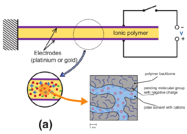
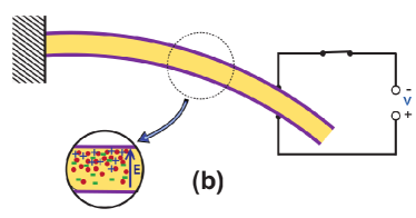
Figure 1: Sketched representation of thin film of EAP : (a) undeformed strip. An inset gives the representative elementary volume (REV) containing the microscopic components of the polymer (Nafion) and (b) the strip bending under an applied electric field.

Electromechanical coupling in ionic polymer membranes was discovered over 50 years ago but has recently received renewed attention due to the development of large strain actuators operating at low electric fields. Modelling of EAP attracts scientists and engineers and a certain number of approaches has been proposed to explain and quantify the physical micro-mechanism which relate the EAP deformation to osmotic diffusion of solvent and ions into the polymer. A micromechanical model has been developed by Nemat-Nasser and Li nemat2000 ; nemat2002 . The model accounts for the electromechanical and chemical-electric coupling of the ion transport, electric field and elastic deformation to produce the response of the EAP. The authors examine the field equations that place the osmotic stress in evidence. They deduce a generalized Darcy’s law and the balance law for the ion flux - a kind of Nernst-Plank equation - deduced from the equation of the electric charge conservation. A first simple macroscopic model was proposed by DeGennes et al. degennes . The model describes the coupling between the electric current density and the solvent (water) flux. Shahinpoor et al. shahinpoor1991 ; shahinpoor1994 ; shahinpoor1998 report the modelling of ion-exchange polymer-metal composites (IPMCs) based on an equation governing the ionic transport mechanism. The authors write down the equations for the solvent concentration, the ionic concentration, and the relationship between stress, strain, electric field, heat flux and chemical energy flux. The stress tensor is related to the deformation gradient field by using a constitutive equation of the neo-Hookean type.

The paper is divided in 8 Sections with 3 appendices. The next section recalls the main results of the previous work Tixier and notations. The section 3 concerns the entropy balance law at the microscopic level and for the whole material over the R.V.E. (Representative Volume Element). The fundamental thermodynamic relations are given in Section 4. The thermodynamic equations are written for each phase (solid, solvent) and then for the complete material leading to Gibb’s relation. On using the latter relation the generalized forces and fluxes are identified in Section 5. The Section 6 is devoted to constitutive equations, especially the tensorial and vectorial constitutive equations are deduced by invoking symmetry properties. A detailed discussion on the results thus obtained is presented in Section 7 and some estimates of the constitutive coefficients are given and compared to the proposed approximations. The paper is closed with a brief conclusion.

2 Modelling and previous results

The system we study is an ionic polymer-metal composite (IPMC); it consists of a polyelectrolyte coated on both sides with thin metal layers acting as electrodes. The electro-active polymer is saturated with water, which results in a quasi-complete dissociation of the polymer : anions remain bound to the polymer backbone, whereas small cations are released in water Futerko . When an electric field perpendicular to the electrodes is applied, the strip bends : cations are attracted by the negative electrode and carry solvent away by osmosis. As a result, the polymer swells near the negative electrode and contracts on the opposite side, leading to the bowing.

The modelling of this system is detailled in our previous article Tixier . The polymer chains are assimilated to a deformable porous medium saturated by an ionic solution composed by water and cations. We suppose that the solution is dilute. We depicted the complete material as the superposition of three systems : a deformable solid made up of polymer backbone negatively charged, a solvent (the water) and cations (see the inset of Fig. 1 for schematic representation). The three components have different velocity fields, and the solid and liquid phases are assumed to be incompressible phases separated by an interface whose thickness is supposed to be negligible. We identify the quantities relative to the different components  by subscripts : $1$ refers to cations, $2$ to solvent, $3$ to solid, $i$ to the interface and $4$ to the solution, that is both components $1$ and $2$; the lack of subscript refers to the complete material. Components $2$, $3$ and $4$ as well as the global material are assimilated to continua. We venture the hypothesis that gravity and magnetic field are negligible, so the only external force acting on the system is the electric force.

We describe this medium using a coarse-grained model developed for two-phase mixtures Nigmatulin79 ; Nigmatulin90 ; Drew83 ; Drew98 ; Ishii06 ; Lhuillier03 . The microscopic scale is large enough to provide the continuum assumption, but small enough to enable the definition of a volume which contains a single phase ($3$ or $4$). At the macroscopic scale, we define a representative elementary volume (R.V.E.) which contains the two phases; it must be small enough so that average quantities relative to the whole material can be considered as local, and large enough so that this average is relevant. A microscale Heaviside-like function of presence $\chi_{k}\left(\mathbf{r},t\right)$ has been defined for the phases $3$ and $4$

$$\chi_{k}=1\;when\;phase\;k\;occupies\;point\;\mathbf{r}\;at\;time\;t,\quad\chi_{k}=0\;otherwise$$ (1)

The function of presence of the interface is the Dirac-like function $\chi_{i}=-\boldsymbol{\nabla}\chi_{k}\cdot\mathbf{n_{k}}$ (in $m^{-1}$) where $\mathbf{n_{k}}$ is the outward-pointing unit normal to the interface in the phase $k$. $\left\langle{}\right\rangle_{k}$ denotes the average over the phase $k$ of a quantity relative to the phase $k$ only. The macroscale quantities relative to the whole material are obtained by statistically averaging the microscale quantities over the R.V.E., that is by repeating many times the same experiment. We suppose that this average, denoted by $\left\langle{}\right\rangle$, is equivalent to a volume average (ergodic hypothesis) and commutes with the space and time derivatives Drew83 ; Lhuillier03 . A macroscale quantity $g_{k}$ verifies

$$g_{k}=\left\langle\chi_{k}g_{k}^{0}\right\rangle=\phi_{k}\left\langle g_{k}^{0}\right\rangle_{k}$$ (2)

where $g_{k}^{0}$ is the corresponding microscale quantity and $\phi_{k}=\left\langle\chi_{k}\right\rangle$ the volume fraction of the phase $k$. In the following, we use superscript ⁰ to indicate microscale quantities; the macroscale quantities, which are averages defined all over the material, are written without superscript.

The conservation and balance laws of the polymer saturated with water have been previously established Tixier . To this end, we supposed that the fluctuations of the following quantities are negligible on the R.V.E. scale : the velocity $\mathbf{V_{k}}$ of each phase and interface, the solid displacement vector $\mathbf{u_{3}}$, the cations molar concentration $C$ and the electric field $\mathbf{E}$. Futhermore, we admitted that the electric field is identical in all the phases and that the solid and liquid phases are isotropic linear dielectrics. We thus established the mass conservation law of the constituents and of the complete material

$$\frac{\partial\rho_{k}}{\partial t}+div\left(\rho_{k}\mathbf{V_{k}}\right)=0\qquad for\;k=2,3$$

(3)

where $\rho_{k}=\phi_{k}\rho_{k}^{0}$ denotes the mass density of the phase $k$ relative to the volume of the whole material. Maxwell’s equations and the constitutive relation can  be written

$$\mathbf{rot}\mathbf{E}=\mathbf{0}\qquad\qquad div\mathbf{D}=\rho Z\qquad\qquad\mathbf{D}=\varepsilon\mathbf{E}$$ (4)

with

$$\varepsilon=\sum\limits_{k=3,4}\phi_{k}\varepsilon_{k}^{0}$$ (5)

where $\mathbf{D}$ is the electric displacement field, $Z$ the total electric charge per unit of mass and $\varepsilon$ the permittivity. The linear momentum and internal energy balance laws are

$$\rho\frac{D\mathbf{V}}{Dt}=\mathbf{div}\boldsymbol{\sigma}+\rho Z\mathbf{E}$$ (6)

$$\rho\frac{D}{Dt}\left(\frac{U_{\Sigma}}{\rho}\right)=\sum\limits_{k=3,4}\left(\boldsymbol{\sigma_{k}}:\boldsymbol{\nabla}\mathbf{V_{k}}\right)+\mathbf{i}\cdot\mathbf{E}-div\mathbf{Q}$$ (7)

where $\boldsymbol{\sigma}$ denotes the stress tensor, $\mathbf{i}$ the diffusion current, $\mathbf{Q}$ the heat flux and $U_{\Sigma}$ the sum of the volume internal energies of the different phases. These two relations use the material derivative $\frac{D}{Dt}$ defined in our previous paper Tixier and reported in appendix A.

The relative velocities of the different phases are negligible compared to the velocities measured in the laboratory-frame. Let’s take for example a strip of Nafion which is $\textit{200}\;\mu m$ thick and $\textit{1.57}\;cm$ long, bending in an electric field. The tip displacement is about $\textit{4}\;mm$ and it is obtained in $\textit{1}\;s$ nemat2000 . The different phases velocities in the laboratory-frame $\left|\mathbf{V_{k}^{0}}\right|$ are close to $\textit{4}\;\textit{10}^{-3}\;m\;s^{-1}$ and the relative velocities $\left|\mathbf{V_{k}^{0}}-\mathbf{V}\right|$ to $\textit{2}\;\textit{10}^{-4}\;m\;s^{-1}$. So we can reasonably suppose that

$$\left|\mathbf{V_{k}^{0}}-\mathbf{V}\right|<<\left|\mathbf{V_{k}^{0}}\right|$$ (8)

The kinetic energy of the whole material is defined either as the sum $E_{c\Sigma}$ of the kinetic energies of the constituents, or as the kinetic energy of the center of mass of the constituents $E_{c}$ Tixier . The difference between these two quantities is

$$E_{c\Sigma}-E_{c}=\frac{\rho_{3}\rho_{4}}{\rho}\left(\mathbf{V_{3}}-\mathbf{V_{4}}\right)^{2}$$ (9)

and is negligible compared to the kinetic energies of each phases. On a first approximation, we can therefore swap together $E_{c\Sigma}$ with $E_{c}$, and consequently $U_{\Sigma}$ with the internal energy of the whole system $U$. Considering this hypothesis, the internal energy balance equation can be written

$$\rho\frac{d}{dt}\left(\frac{U}{\rho}\right)=\boldsymbol{\sigma}:\boldsymbol{\nabla}\mathbf{V}+\mathbf{i^{\prime}}\cdot\mathbf{E}-div\mathbf{Q^{\prime}}$$ (10)

with

$$\mathbf{i^{\prime}}=\mathbf{I}-\rho Z\mathbf{V}\simeq\rho_{1}Z_{1}\left(\mathbf{V_{1}}-\mathbf{V_{4}}\right)+\sum\limits_{k=3,4}\rho_{k}Z_{k}\left(\mathbf{V_{k}}-\mathbf{V}\right)$$

(11)

where $\mathbf{I}$ denotes the current density vector and

$$Z_{k}=Z_{k}^{0}\qquad for\;k=1,2,3\qquad\ and\qquad Z_{4}=\frac{\rho_{1}}{\rho_{4}}Z_{1}$$ (12)

To describe the systeme, we finally have 14 independent scalar equations using 29 scalar variables ($\rho_{k}$, $\mathbf{V_{k}}$ ($k=1,3$), $\rho$, $\mathbf{V}$, $\boldsymbol{\sigma}$, $Z$, $\mathbf{E}$, $U$, $\mathbf{Q^{\prime}}$ and $\mathbf{D}$). 15 scalar equations are missing to close the system : the constitutive relations. We will now establish them in the form of three vectorial relations and one tensorial relation relating second-rank symmetric tensors.

3 Entropy balance law

The microscale entropy balance laws of the solid and liquid phases can be written

$$\frac{\partial S_{k}^{0}}{\partial t}+divS_{k}^{0}\mathbf{V_{k}^{0}}=-div\mathbf{\Sigma_{k}^{0}}+s_{k}^{0}\qquad\qquad k=3,4$$ (13)

where $S_{k}^{0}$, $\mathbf{\Sigma_{k}^{0}}$ and $s_{k}^{0}$ denote, respectively, the entropy density, the entropy flux vector and the rate of entropy production of the phase $k$.

Averaging over the R.V.E. gives, considering the interface condition $\mathbf{V_{1}^{0}}=\mathbf{V_{2}^{0}}=\mathbf{V_{3}^{0}}=\mathbf{V_{4}^{0}}=\mathbf{V_{i}^{0}}$

$$\frac{\partial S_{k}}{\partial t}+div\left(S_{k}\mathbf{V_{k}}\right)=s_{k}-div\mathbf{\Sigma_{k}}-\left\langle\mathbf{\Sigma_{k}^{0}}\cdot\mathbf{n_{k}}\chi_{i}\right\rangle$$ (14)

in which the macroscale entropy density $S_{k}$, the entropy flux vector $\mathbf{\Sigma_{k}}$ and the rate of entropy production $s_{k}$ are defined by

$$S_{k}=\left\langle\chi_{k}S_{k}^{0}\right\rangle\qquad\qquad\mathbf{\Sigma_{k}}=\left\langle\chi_{k}\mathbf{\Sigma_{k}^{0}}\right\rangle\qquad\qquad s_{k}=\left\langle\chi_{k}s_{k}^{0}\right\rangle$$ (15)

One points out that the quantities $S_{k}$ and $s_{k}$ are relative to the volume of the whole material. For the interface we obtain (see appendix B)

$$\frac{\partial S_{i}}{\partial t}+div\left(S_{i}\mathbf{V_{i}}\right)=\sum\limits_{k=3,4}\left\langle\chi_{i}\mathbf{\Sigma_{k}^{0}}\cdot\mathbf{n_{k}}\right\rangle+s_{i}$$ (16)

The entropy balance law of the whole material is

$$\rho\frac{D}{Dt}\left(\frac{S}{\rho}\right)=s-div\mathbf{\Sigma}$$ (17)

where :

$$S=\sum\limits_{k=3,4,i}S_{k}\qquad\qquad s=\sum\limits_{k=3,4,i}s_{k}\qquad\qquad\mathbf{\Sigma}=\sum\limits_{k=3,4}\mathbf{\Sigma_{k}}$$ (18)

are the entropy density, the rate of entropy production and the entropy flux vector of the complete material, respectively. In the barycentric frame of reference, we derive

$$\rho\frac{d}{dt}\left(\frac{S}{\rho}\right)=s-div\mathbf{\Sigma^{\prime}}$$ (19)

with

$$\mathbf{\Sigma^{\prime}}=\mathbf{\Sigma}-\sum\limits_{k=3,4}S_{k}\left(\mathbf{V}-\mathbf{V_{k}}\right)$$ (20)

4 Fundamental thermodynamic relations

4.1 Thermodynamic relations for the solide phase

For a solid phase with one constituent, the Gibb’s relation can be written DeGroot

$$\rho_{3}^{0}\frac{d_{3}^{0}}{dt}\left(\frac{U_{3}^{0}}{\rho_{3}^{0}}\right)=p_{3}^{0}\frac{1}{\rho_{3}^{0}}\frac{d_{3}^{0}\rho_{3}^{0}}{dt}+\boldsymbol{\sigma_{3}^{0e}}^{s}:\frac{d_{3}^{0}\boldsymbol{\varepsilon_{3}^{0}}^{s}}{dt}+\rho_{3}^{0}T_{3}^{0}\frac{d_{3}^{0}}{dt}\left(\frac{S_{3}^{0}}{\rho_{3}^{0}}\right)$$ (21)

where $T_{3}^{0}$ is the absolute temperature, $\boldsymbol{\varepsilon_{3}^{0}}$ the strain tensor, $\boldsymbol{\sigma_{3}^{0e}}$ the equilibrium stress tensor, $\boldsymbol{\sigma_{3}^{0e}}^{s}$ and $\boldsymbol{\varepsilon_{3}^{0}}^{s}$ the stress and strain deviator tensors, and $\frac{d_{3}^{0}}{dt}$ the particule derivative following the microscale motion of the solid (see appendix A). $p_{3}^{0}$ is the pressure or negative one-third the trace of the microscopic equilibrium stress tensor

$$p_{3}^{0}=-\frac{1}{3}tr\left(\boldsymbol{\sigma_{3}^{0e}}\right)$$ (22)

Equation (21) can also be deduced from equation (13) and internal energy balance equation of the solid phase developped in Tixier : indeed, the Gibbs relation is satisfied at equilibrium, so the heat flux $\mathbf{Q_{3}^{0}}$, the diffusion current $\mathbf{i_{3}^{0}}$ and the rate of entropy production $s_{3}^{0}$ cancel; deformations are small and the stress tensor $\boldsymbol{\sigma_{3}^{0}}$ is equal to the equilibrium stress tensor $\boldsymbol{\sigma_{3}^{0e}}$. In addition, the solid phase is a closed system, consequently

$$\mathbf{\Sigma_{3}^{0}}=\frac{\mathbf{Q_{3}^{0}}}{T_{3}^{0}}$$ (23)

At the microscopic scale, Euler’s homogeneous function theorem provides for the solid phase

$$p_{3}^{0}=T_{3}^{0}S_{3}^{0}-U_{3}^{0}+\mu_{3}^{0}\rho_{3}^{0}$$ (24)

where $\mu_{3}^{0}$ denotes the chemical potential per unit of mass of the solid constituent. As a result, Gibbs equation can be written

$$\frac{d_{3}^{0}U_{3}^{0}}{dt}=T_{3}^{0}\frac{d_{3}^{0}S_{3}^{0}}{dt}+\mu_{3}^{0}\frac{d_{3}^{0}\rho_{3}^{0}}{dt}+\boldsymbol{\sigma_{3}^{0e}}^{s}:\frac{d_{3}^{0}}{dt}\boldsymbol{\varepsilon_{3}^{0}}^{s}$$ (25)

Differentiating Euler’s relation and combining it with the Gibbs relation leads to Gibbs-Duhem equation

$$\frac{d_{3}^{0}p_{3}^{0}}{dt}=S_{3}^{0}\frac{d_{3}^{0}T_{3}^{0}}{dt}-\boldsymbol{\sigma_{3}^{0e}}^{s}:\frac{d_{3}^{0}}{dt}\boldsymbol{\varepsilon_{3}^{0}}^{s}+\rho_{3}^{0}\frac{d_{3}^{0}\mu_{3}^{0}}{dt}$$ (26)

Let us assume that the fluctuations over the R.V.E. of the intensive thermodynamical quantities $T_{3}^{0}$, $\mu_{3}^{0}$, $p_{3}^{0}$, the displacement $\mathbf{u_{3}^{0}}$ and the equilibrium stress tensor $\boldsymbol{\sigma_{3}^{0e}}$ are negligible. Supposing that the solid deformations are small, we obtain

$$T_{3}=T_{3}^{0}\qquad\qquad\mu_{3}=\mu_{3}^{0}$$ (27)

$$\mathbf{u_{3}}=\mathbf{u_{3}^{0}}\qquad\qquad\boldsymbol{\varepsilon_{3}}=\boldsymbol{\varepsilon_{3}^{0}}=\frac{1}{2}\left(\boldsymbol{\nabla}\mathbf{u_{3}}+\boldsymbol{\nabla}\mathbf{u_{3}}^{T}\right)$$ (28)

$$p_{3}=p_{3}^{0}=-\frac{1}{3\phi_{3}}tr\boldsymbol{\sigma_{3}^{e}}\qquad\qquad\boldsymbol{\sigma_{3}^{e}}=\phi_{3}\boldsymbol{\sigma_{3}^{0e}}=\boldsymbol{\sigma_{3}^{e}}^{s}-\phi_{3}p_{3}\boldsymbol{1}$$ (29)

where $\boldsymbol{1}$ denotes the second-rank identity tensor and $\boldsymbol{\sigma_{3}^{e}}^{s}$ the deviator part of $\boldsymbol{\sigma_{3}^{e}}$. Considering the small deformation hypothesis, one easily derives (cf appendix C)

$$\frac{d_{3}U_{3}}{dt}=T_{3}\frac{d_{3}S_{3}}{dt}+\mu_{3}\frac{d_{3}\rho_{3}}{dt}-p_{3}\frac{d_{3}\phi_{3}}{dt}+\boldsymbol{\sigma_{3}^{e}}^{s}:\frac{d_{3}}{dt}\boldsymbol{\varepsilon_{3}}^{s}$$ Gibbs

Euler

Gibbs-Duhem

(30)

4.2 Thermodynamic relations for the liquid phase

According to S.R. De Groot and P. Mazur DeGroot , the Gibbs relation of a two-constituent fluid can be written as

$$\frac{d_{4}^{0}}{dt}\left(\frac{U_{4}^{0}}{\rho_{4}^{0}}\right)=T_{4}^{0}\frac{d_{4}^{0}}{dt}\left(\frac{S_{4}^{0}}{\rho_{4}^{0}}\right)-p_{4}^{0}\frac{d_{4}^{0}}{dt}\left(\frac{1}{\rho_{4}^{0}}\right)+\sum\limits_{k=1,2}\mu_{k}^{0}\frac{d_{4}^{0}}{dt}\left(\frac{\rho_{k}^{\prime}}{\rho_{4}^{0}}\right)$$ (31)

where $p_{4}^{0}$ is the fluid phase pressure, $\mu_{k}^{0}$ the mass chemical potential of constituent $k$, and $\frac{d_{4}^{0}}{dt}$ the particule derivative following the microscale motion of the liquid phase. $\rho_{k}^{\prime}$ are the mass densities of cations and solvent relative to the solution volume

$$\frac{\rho_{k}^{\prime}}{\rho_{4}^{0}}=\frac{\rho_{k}}{\rho_{4}}\qquad$$

(32)

$M_{1}$ denotes the cations molar mass and $C$ the cations molar concentration relative to the liquid phase. As for the solid phase, one can find out this equation combining the internal energy and entropy balance laws and taking the limit at the equilibrium. Euler’s homogeneous function theorem takes on the following form at the microscopic scale

$$U_{4}^{0}-T_{4}^{0}S_{4}^{0}+p_{4}^{0}=\sum\limits_{k=1,2}\mu_{k}^{0}\rho_{k}^{\prime}$$ (33)

so that

$$\frac{d_{4}^{0}U_{4}^{0}}{dt}=T_{4}^{0}\frac{d_{4}^{0}S_{4}^{0}}{dt}+\sum\limits_{k=1,2}\mu_{k}^{0}\frac{d_{4}^{0}\rho_{k}^{\prime}}{dt}$$ (34)

The Gibbs-Duhem relation of the liquid phase derives from the Gibbs and Euler’s relations

$$\sum\limits_{k=1,2}\rho_{k}^{\prime}\frac{d_{4}^{0}\mu_{k}^{0}}{dt}=-S_{4}^{0}\frac{d_{4}^{0}T_{4}^{0}}{dt}+\frac{d_{4}^{0}p_{4}^{0}}{dt}$$ (35)

We assume that the fluctuations of the intensive thermodynamic quantities are negligible

$$T_{4}=T_{4}^{0}\qquad\qquad\mu_{k}=\mu_{k}^{0}\qquad\qquad p_{4}=p_{4}^{0}$$ (36)

Averaging the previous equations over the R.V.E., we obtain

$$T_{4}\frac{d_{4}S_{4}}{dt}=\frac{d_{4}U_{4}}{dt}+p_{4}\frac{d_{4}\phi_{4}}{dt}-\sum\limits_{k=1,2}\mu_{k}\frac{d_{4}\rho_{k}}{dt}$$ Gibbs

Euler

Gibbs-Duhem

(37)

4.3 Thermodynamic relations for the complete material

In order to write the thermodynamic relations of the complete material, we make the hypothesis of local thermodynamic equilibrium; this requires among other things that the heat diffuses well enough in the solid and the solution so that temperature equilibrium is reached on the R.V.E.. We thus can write

$$p=p_{3}=p_{4}$$

(38)

Otherwise, we have pointed out that the sum $U_{\Sigma}$ of the internal energies of the constituents is close to the internal energy of the system $U$. Adding the Euler’s relations of the solid and the liquid phases and the interface, we thus obtain the Euler’s relation of the whole material

$$p=TS-U+\sum\limits_{k=1,2,3}\mu_{k}\rho_{k}$$ (39)

The Gibbs relation of the complete material is also obtained by addition

$$T\frac{D}{Dt}\left(\frac{S}{\rho}\right)=\frac{D}{Dt}\left(\frac{U}{\rho}\right)+p\frac{D}{Dt}\left(\frac{1}{\rho}\right)-\frac{1}{\rho}\boldsymbol{\sigma_{3}^{e}}^{s}:\frac{d_{3}\boldsymbol{\varepsilon_{3}}^{s}}{dt}-\sum\limits_{1,2}\mu_{k}\frac{\rho_{4}}{\rho}\frac{d_{4}}{dt}\left(\frac{\rho_{k}}{\rho_{4}}\right)$$ (40)

The material derivative enables to follow the barycenters of each phase during the motion. The solid phase is then supposed to be a closed system; for this reason, no mass exchange term for the solid appears in this relation. On the contrary, the solvent and the cations move at different velocities; thence there is a mass exchange term concerning these two constituents in the barycentric reference frame of the solution. The mass exchanges of the three constituents appear if the particle derivative following the motion of the whole material barycenter is used

$$T\frac{d}{dt}\left(\frac{S}{\rho}\right)=\frac{d}{dt}\left(\frac{U}{\rho}\right)+p\frac{d}{dt}\left(\frac{1}{\rho}\right)-\sum\limits_{k=1,2,3}\mu_{k}\frac{d}{dt}\left(\frac{\rho_{k}}{\rho}\right)-\frac{1}{\rho}\boldsymbol{\sigma_{3}^{e}}^{s}:\frac{d\boldsymbol{\varepsilon_{3}}^{s}}{dt}$$ (41)

This relation can also be obtained using the Gibbs relations of the constituents; at equilibrium, indeed, the velocities of the two phases and the interface are identical, in such a way that the particle derivatives are the same

$$\frac{d_{3}}{dt}\equiv\frac{d_{4}}{dt}\equiv\frac{d_{i}}{dt}\equiv\frac{d}{dt}$$ (42)

A third approach is to combine the balance equations of internal energy and entropy of the complete material, and to take the limit at equilibrium.

Considering the small deformations hypothesis and neglecting the relative velocities compared to the velocities in the laboratory-frame, we derive

$$\boldsymbol{\sigma_{3}^{e}}^{s}:\boldsymbol{\nabla}\mathbf{V_{3}}=\boldsymbol{\sigma_{3}^{e}}^{s}:\frac{d_{3}\boldsymbol{\varepsilon_{3}}^{s}}{dt}\simeq\boldsymbol{\sigma_{3}^{e}}^{s}:\frac{d\boldsymbol{\varepsilon_{3}}^{s}}{dt}\simeq\boldsymbol{\sigma_{3}^{e}}^{s}:\boldsymbol{\nabla}\mathbf{V}$$ (43)

The equilibrium stress tensor of the complete material is written as follows

$$\boldsymbol{\sigma^{e}}=\boldsymbol{\sigma_{3}^{e}}+\boldsymbol{\sigma_{4}^{e}}=-p\boldsymbol{1}+\boldsymbol{\sigma_{3}^{e}}^{s}$$ (44)

with

$$\boldsymbol{\sigma_{4}^{e}}=-\phi_{4}p_{4}\boldsymbol{1}$$ (45)

As a result

$$\boldsymbol{\sigma^{e}}^{s}=\boldsymbol{\sigma_{3}^{e}}^{s}$$ (46)

Finally, Gibbs relation is

$$T\frac{d}{dt}\left(\frac{S}{\rho}\right)=\frac{d}{dt}\left(\frac{U}{\rho}\right)+p\frac{d}{dt}\left(\frac{1}{\rho}\right)-\sum\limits_{k=1,2,3}\mu_{k}\frac{d}{dt}\left(\frac{\rho_{k}}{\rho}\right)-\frac{1}{\rho}\boldsymbol{\sigma^{e}}^{s}:\boldsymbol{\nabla}\mathbf{V}$$ (47)

Differentiating Euler’s relation and combining it with Gibbs relation, the Gibbs-Duhem relation takes on the form

$$\frac{dp}{dt}=S\frac{dT}{dt}+\sum\limits_{k=1,2,3}\rho_{k}\frac{d\mu_{k}}{dt}-\boldsymbol{\sigma^{e}}^{s}:\boldsymbol{\nabla}\mathbf{V}$$ (48)

5 Generalized forces and fluxes

5.1 Entropy production

The stress tensor is composed of two parts : the equilibrium stress tensor $\boldsymbol{\sigma^{e}}$ and the viscous stress tensor $\boldsymbol{\sigma^{v}}$, which vanishes at equilibrium. Considering (44), the complete stress tensor can be written as

$$\boldsymbol{\sigma}=\boldsymbol{\sigma_{3}}+\boldsymbol{\sigma_{4}}=\boldsymbol{\sigma^{e}}+\boldsymbol{\sigma^{v}}=-p\boldsymbol{1}+\boldsymbol{\sigma^{e}}^{s}+\boldsymbol{\sigma^{v}}$$ (49)

Combining the internal energy and entropy equations (10) and (19) with the Gibbs relation (47) yields

$$s-div\mathbf{\Sigma^{\prime}}=\frac{1}{T}\boldsymbol{\sigma^{v}}:\boldsymbol{\nabla}\mathbf{V}+\frac{1}{T}\mathbf{i^{\prime}}\cdot\mathbf{E}-\frac{1}{T^{2}}\mathbf{Q^{\prime}}\cdot\boldsymbol{\nabla}T$$

(50)

We can then identify the rate of entropy production $s$ and the entropy flux vector $\mathbf{\Sigma^{\prime}}$

$$s=\frac{1}{T}\boldsymbol{\sigma^{v}}:\boldsymbol{\nabla}\mathbf{V}+\frac{1}{T}\mathbf{i^{\prime}}\cdot\mathbf{E}-\frac{1}{T^{2}}\mathbf{Q^{\prime}}\cdot\boldsymbol{\nabla}T+\sum\limits_{k=1,2,3}\rho_{k}\left(\mathbf{V}-\mathbf{V_{k}}\right)\cdot\boldsymbol{\nabla}\frac{\mu_{k}}{T}$$

(51)

5.2 Identification of the generalized forces and fluxes

A second rank tensor is the sum of three parts : a spherical tensor, a deviator tensor (labeled with ^s) and an antisymmetric tensor (labeled with ^a)

$$\boldsymbol{\nabla}\mathbf{V}=\frac{1}{3}\left(div\mathbf{V}\right)\boldsymbol{1}+\boldsymbol{\nabla}\mathbf{V}^{s}+\boldsymbol{\nabla}\mathbf{V}^{a}$$ (52)

where

$$\boldsymbol{\nabla}\mathbf{V}^{s}=\frac{1}{2}\left(\boldsymbol{\nabla}\mathbf{V}+\boldsymbol{\nabla}\mathbf{V}^{T}\right)-\frac{1}{3}\left(div\mathbf{V}\right)\boldsymbol{1}$$ (53)

The viscous stress tensor is symmetric, so

$$\boldsymbol{\sigma^{v}}=\frac{1}{3}tr\left(\boldsymbol{\sigma^{v}}\right)\boldsymbol{1}+\boldsymbol{\sigma^{v}}^{s}$$ (54)

In the entropy production $s$ appear the three mass diffusion fluxes relative to the barycentric reference frame $\rho_{k}\left(\mathbf{V_{k}}-\mathbf{V}\right)$ with $k=1,2,3$. The sum of these three fluxes is zero, so only two of them are linearly independant. We define the following equivalent fluxes

$$\mathbf{J_{1}}=\rho_{1}\left(\mathbf{V_{1}}-\mathbf{V_{2}}\right)\qquad\qquad\qquad\mathbf{J_{4}}=\rho_{4}\left(\mathbf{V_{4}}-\mathbf{V_{3}}\right)$$ (55)

which are respectively the mass diffusion flux of the cations in the solution and the mass diffusion flux of the solution in the solid. These two fluxes are linearly independant. The diffusion current $\mathbf{i^{\prime}}$ and the fluxes $\rho_{k}\left(\mathbf{V_{k}}-\mathbf{V}\right)$ can be expressed as functions of $\mathbf{J_{1}}$ and $\mathbf{J_{4}}$, then the entropy production takes on the following form

$$s$$

(56)

This expression places in evidence one scalar flux $\frac{1}{3}tr\left(\boldsymbol{\sigma^{v}}\right)$, three vectorial fluxes $\mathbf{Q^{\prime}}$, $\mathbf{J_{1}}$, $\mathbf{J_{4}}$ and one second-rank tensorial flux $\boldsymbol{\sigma^{v}}^{s}$ along with the associated generalized forces

Fluxes Forces

$$\frac{1}{3}tr\boldsymbol{\sigma^{v}}$$

(57)

6 Constitutive equations

6.1 Tensorial constitutive equation

We assume that the medium is isotropic. According to Curie dissymmetry principle, there can not be any coupling between fluxes and forces whose tensorial ranks differs from one unit. Moreover, we suppose that coupling between fluxes and different tensorial rank forces are negligible, which is a generally accepted hypothesis DeGroot . Consequently, the scalar constitutive equation requires only one scalar phenomenological coefficient $L_{1}$

$$\frac{1}{3}tr\left(\boldsymbol{\sigma^{v}}\right)=\frac{L_{1}}{T}div\mathbf{V}$$ (58)

In the same way, the tensorial flux $\boldsymbol{\sigma^{v}}^{s}$ is related to the generalized force $\frac{1}{T}\boldsymbol{\nabla}\mathbf{V}^{s}$ by a fourth-rank tensorial phenomenological coefficient $\boldsymbol{L_{2}}$

$$\boldsymbol{\sigma^{v}}^{s}=\boldsymbol{L_{2}}\frac{1}{T}\mathbf{\boldsymbol{\nabla}V}^{s}$$ (59)

Because of the isotropy of the medium, tensor $\boldsymbol{L_{2}}$ is isotropic and requires only three scalar coefficients DeGroot . Furthermore, tensors $\boldsymbol{\sigma^{v}}^{s}$ and $\boldsymbol{\nabla}\mathbf{V}^{s}$ are deviatoric, so

$$\boldsymbol{\sigma^{v}}^{s}=\frac{L_{2}}{T}\boldsymbol{\nabla}\mathbf{V}^{s}$$ (60)

where $L_{2}$ is a scalar coefficient. Setting out $L_{1}^{\prime}=L_{1}-\frac{L_{2}}{3}$, the viscous stress tensor is finally given by

$$\boldsymbol{\sigma^{v}}=\frac{L_{1}^{\prime}}{T}\left(div\mathbf{V}\right)\boldsymbol{1}+\frac{L_{2}}{2T}\left(\boldsymbol{\nabla}\mathbf{V}+\boldsymbol{\nabla}\mathbf{V}^{T}\right)$$ (61)

Assuming that the complete material satisfies the Hooke’s law at equilibrium, the equilibrium stress tensor can be written as

$$\boldsymbol{\sigma^{e}}=\lambda\left(tr\boldsymbol{\varepsilon}\right)\boldsymbol{1}+2G\boldsymbol{\varepsilon}=\frac{3\lambda+2G}{3}\left(tr\boldsymbol{\varepsilon}\right)\boldsymbol{1}+2G\boldsymbol{\varepsilon}^{s}$$ (62)

where $\lambda$ and $G$ denote the first Lamé constant and the shear modulus of the complete material, respectively, and where the material strain is defined by

$$\boldsymbol{\varepsilon}=\frac{1}{2}\left(\boldsymbol{\nabla}\mathbf{u}+\boldsymbol{\nabla}\mathbf{u}^{T}\right)\qquad or\qquad\overset{\bullet}{\boldsymbol{\varepsilon}}=\frac{1}{2}\left(\boldsymbol{\nabla}\mathbf{V}+\boldsymbol{\nabla}\mathbf{V}^{T}\right)$$ (63)

$\mathbf{u}$ is the displacement vector. Supposing that the fluid is newtonian and stokesian, the pressure is

$$p=-\frac{1}{3}tr\left(\boldsymbol{\sigma^{e}}\right)=\left(\lambda+\frac{2}{3}G\right)tr\boldsymbol{\varepsilon}$$ (64)

The stress tensor of the complete material thus satisfies a Kelvin-Voigt model

$$\boldsymbol{\sigma}=\lambda\left(tr\boldsymbol{\varepsilon}\right)\boldsymbol{1}+2G\boldsymbol{\varepsilon}+\frac{L_{1}^{\prime}}{T}\left(tr\overset{\bullet}{\boldsymbol{\varepsilon}}\right)\boldsymbol{1}+\frac{L_{2}}{T}\overset{\bullet}{\boldsymbol{\varepsilon}}$$ (65)

6.2 Chemical potentials

The liquid phase is a dilute solution of strong electrolyte. Molar chemical potentials of the three constituents $\mu_{i,mol}$ can be written on a first approximation Diu

$$\mu_{1,mol}\left(T,p,x\right)=\mu_{1,mol}^{0}\left(T,p\right)+RT\ln x+o(\sqrt{x})$$

(66)

where $R=8,314\;J\;K^{-1}$ is the gas constant and $x$ the molar fraction of the cations in the solution

$$x=C\frac{M_{2}}{\rho_{2}^{0}}$$ (67)

$\mu_{2,mol}^{0}$ and $\mu_{3,mol}^{0}$ denote the chemical potentials of the single solid and solvent, and $\mu_{1,mol}^{0}$ depends on the solvent and the solute. Mass chemical potentials $\mu_{i}=\frac{\mu_{i,mol}}{M_{i}}$ can then be written

$$\mu_{1}\left(T,p,x\right)\simeq\mu_{1}^{0}\left(T,p\right)+\frac{RT}{M_{1}}\ln\left(C\frac{M_{2}}{\rho_{2}^{0}}\right)$$

(68)

Using the Gibbs-Duhem’s relations for the solid and the liquid phases, we obtain

$$\boldsymbol{\nabla}\mu_{1}=-\frac{S_{1}}{\rho_{1}}\boldsymbol{\nabla}T+\frac{v_{1}}{M_{1}}\boldsymbol{\nabla}p+\frac{RT\rho_{2}^{0}}{M_{2}M_{1}C}\boldsymbol{\nabla}\left(\frac{CM_{2}}{\rho_{2}^{0}}\right)$$

(69)

where $v_{i}$ denotes the partial molar volume of the constituent $i$.

6.3 Vectorial constitutive equations

Vectorial constitutive equations require nine phenomenogical coefficients. These coefficients are a priori second-rank tensors; considering the isotropy of the medium, they can be replaced by scalars

$$\mathbf{Q^{\prime}}=L_{3}\boldsymbol{\nabla}\frac{1}{T}+L_{4}\frac{\rho_{2}}{\rho_{4}}\left[\frac{1}{T}Z_{1}\mathbf{E}-\boldsymbol{\nabla}\frac{\mu_{1}}{T}+\boldsymbol{\nabla}\frac{\mu_{2}}{T}\right]$$

(70)

$$\mathbf{J_{1}}=L_{4}\boldsymbol{\nabla}\frac{1}{T}+L_{7}\frac{\rho_{2}}{\rho_{4}}\left[\frac{1}{T}Z_{1}\mathbf{E}-\boldsymbol{\nabla}\frac{\mu_{1}}{T}+\boldsymbol{\nabla}\frac{\mu_{2}}{T}\right]$$

(71)

$$\mathbf{J_{4}}=L_{5}\boldsymbol{\nabla}\frac{1}{T}+L_{8}\frac{\rho_{2}}{\rho_{4}}\left[\frac{1}{T}Z_{1}\mathbf{E}-\boldsymbol{\nabla}\frac{\mu_{1}}{T}+\boldsymbol{\nabla}\frac{\mu_{2}}{T}\right]$$

(72)

Onsager reciprocal relations lead otherwise to

$$L_{6}=L_{4}\qquad\qquad L_{9}=L_{5}\qquad\qquad L_{10}=L_{8}$$ (73)

Considering that the solution is dilute and using the expressions obtained for the chemical potentials, the heat flux writes

$$\mathbf{Q^{\prime}}=-\frac{A_{QT}}{T^{2}}\boldsymbol{\nabla}T+\frac{A_{QE}}{T}\mathbf{E}+\frac{A_{QP}}{T}\boldsymbol{\nabla}p+A_{QC}\boldsymbol{\nabla}C$$ (74)

with

$$A_{QT}\simeq L_{3}+L_{4}\left[-\mu_{1}^{0}-\frac{RT}{M_{1}}\ln\left(\frac{CM_{2}}{\rho_{2}^{0}}\right)+\mu_{2}^{0}-\frac{RT}{\rho_{2}^{0}}C-\frac{S_{1}T}{\rho_{1}}+\frac{S_{2}T}{\rho_{2}}\right]$$

(75)

According to the definition of the partial molar volumes, indeed

$$\rho_{1}\frac{v_{1}}{{}_{M_{1}}}+\rho_{2}\frac{v_{2}}{{}_{M_{2}}}=\phi_{4}$$ (76)

Likewise, the mass diffusion flux of the cations in the solution can be written as

$$\mathbf{J_{1}}=-\frac{A_{1T}}{T^{2}}\boldsymbol{\nabla}T+\frac{A_{1E}}{T}\mathbf{E}+\frac{A_{1P}}{T}\boldsymbol{\nabla}p+A_{1C}\boldsymbol{\nabla}C$$ (77)

with

$$A_{1T}\simeq L_{4}+L_{7}\left(\mu_{2}^{0}-\mu_{1}^{0}-\frac{RT}{M_{1}}\ln\frac{CM_{2}}{\rho_{2}^{0}}-\frac{RTC}{\rho_{2}^{0}}+T\frac{S_{2}}{\rho_{4}}-T\frac{S_{1}}{\rho_{1}}\right)$$

(78)

and the mass diffusion flux of the solution in the solid is

$$\mathbf{J_{4}}=-\frac{A_{4T}}{T^{2}}\boldsymbol{\nabla}T+\frac{A_{4E}}{T}\mathbf{E}+\frac{A_{4P}}{T}\boldsymbol{\nabla}p+A_{4C}\boldsymbol{\nabla}C$$ (79)

with

$$A_{4T}\simeq L_{5}+L_{8}\left[\mu_{2}^{0}-\frac{RT}{\rho_{2}^{0}}C-\mu_{1}^{0}-\frac{RT}{M_{1}}\ln\left(C\frac{M_{2}}{\rho_{2}^{0}}\right)-\frac{TS_{1}}{\rho_{1}}+\frac{TS_{2}}{\rho_{2}}\right]$$

(80)

7 Discussion

7.1 Nafion physicochemical properties

In order to approximate these complex equations, we are going to estimate the different terms. To do this, we focus on a particular electroactive polymer, Nafion, and we restrict ourself to the isothermal case.

The physicochemical properties of the dry polymer are well documented; its molecular weight $M_{3}$ is between $\textit{10}^{\textit{2}}$ and $\textit{10}^{\textit{3}}\;kg\;mol^{-1}$ Heitner-Wirguin and its mass density $\rho_{3}^{0}$ is close to $\textit{2.1}\;\textit{10}^{\textit{3}}\;kg\;m^{-3}$ nemat2000 . Its equivalent weight $M_{eq}$, that is to say, the weight of polymer per mole of ionic sites is $\textit{1.1}\;kg\;eq^{-1}$ Gebel . We deduce the electric charge per unit of mass $Z_{3}=-\frac{F}{M_{eq}}=\textit{9}\;\textit{10}^{\textit{4}}\;C\;kg^{-1}$ where $F=\textit{96487}\;C\;mol^{-1}$ denotes the Faraday’s constant. The cations may be $H^{+}$, $Li^{+}$ or $Na^{+}$ ions; we use an average molar mass $M_{1}\sim\textit{10}^{\textit{-2}}\;kg\;mol^{-1}$, which corresponds to a mass electric charge $Z_{1}\sim\textit{10}^{\textit{7}}\;C\;kg^{-1}$. The cations partial molar volume $v_{1}$ is on the order of $\frac{M_{1}}{\rho_{4}^{0}}\sim\textit{10}^{\textit{-5}}\;m^{3}\;mol^{-1}$. The solvent molar mass $M_{2}$ is equal to $\textit{18}\;\textit{10}^{\textit{-3}}\;kg\;mol^{-1}$ and its mass density $\rho_{2}^{0}$  is $\textit{10}^{\textit{3}}\;kg\;m^{-3}$; its partial molar volume $v_{2}$ is approximately equal to $\textit{18}\;\textit{10}^{\textit{-6}}\;m^{3}\;mol^{-1}$, which is the molar volume of pure solvent. The dynamic viscosity of water $\eta_{2}$ is $\textit{10}^{\textit{-3}}\;Pa\;s$.

When the polymer is saturated with water, the solution mass fraction is usually between 20% and 25% if the counterion is a proton Cappadonia . It corresponds to a volume fraction $\phi_{4}$ between 34% and 41%. According to P. Choi Choi , each anion is then surrounded by an average of $14$ molecules of water, which corresponds to a porosity of 32%. In the case of a counterion $Li^{+}$ or $Na^{+}$, S. Nemat-Nasser and J. Yu Li nemat2000 indicate that the volume increases by 44.3% and 61.7% respectively between the dry and the saturated polymer, which corresponds to porosities equal to 31% and 38%. Thereafter we use an average value $\phi_{4}\sim\textit{35\%}$. We deduce the mass densities of the complete material, cations, solvent and solid relative to the volume of the whole material

$$\rho_{1}\sim 14\;kg\;m^{-3}\qquad\qquad$$

(81)

The cations molar fraction relative to the liquid phase and the anions molar concentration, which is equal to the average cations concentration, can be written

$$x\sim 7\%\qquad\qquad C\sim 4\;10^{3}\;mol\;m^{-3}$$ (82)

In the following, we suppose that the temperature is $T=\textit{300}\;K$. Regarding to the electric field, it is typically about $\textit{10}^{\textit{4}}\;V\;m^{-1}$ nemat2000 .

7.2 Rheological equation

We have shown that the rheological equation of the complete material is identified with a Kelvin-Voigt model

$$\boldsymbol{\sigma}=\lambda\left(tr\boldsymbol{\varepsilon}\right)\boldsymbol{1}+2G\boldsymbol{\varepsilon}+\lambda_{v}\left(tr\overset{\bullet}{\boldsymbol{\varepsilon}}\right)\boldsymbol{1}+2\mu_{v}\overset{\bullet}{\boldsymbol{\varepsilon}}$$ (83)

where $\lambda$ and $G$ are respectively the first Lamé constant and the shear modulus of the whole material. $\lambda_{v}$ and $\mu_{v}$ are viscoelastic coefficients

$$\lambda_{v}\equiv\frac{L_{1}^{\prime}}{T}\qquad\qquad 2\mu_{v}\equiv\frac{L_{2}}{T}$$ (84)

Nafion is a thermoplastic semi-crystalline ionomer. M. N. Silberstein and M. C. Boyce represent the polymer by a Zener model Silberstein2010 . The elastic coefficients of the dry polymer can be deduced from their measures

$$G_{3}\sim 1.1\;10^{8}\;Pa\qquad\lambda_{3}\sim 2.6\;10^{8}\;Pa\qquad E_{3}\sim 3\;10^{8}\;Pa\qquad\nu_{3}\sim 0.36$$ (85)

where $G_{3}$ is the shear modulus, $\lambda_{3}$ the first Lamé constant, $E_{3}$ the Young’s modulus and $\nu_{3}$ the Poisson’s ratio of the solid phase. Young’s modulus is in good agreement with the values cited in Satterfield2009 . They also correspond to the typical values of this kind of polymer, especially Poisson’s ratio, which is usually close to 0.33 below the glass transition temperature and to 0.5 around the transition temperature ferry .

When the polymer is saturated with water, the elastic coefficients vary; water has a plasticising effect Kundu ; Bauer . We obtain the following values Silberstein2010 ; Satterfield2009 ; Bauer , which are in agreement with the usual ones ferry

$$G\sim 4.5\;10^{7}\;Pa\qquad\lambda\sim 3\;10^{8}\;Pa\qquad E\sim 1.3\;10^{8}\;Pa\qquad\nu\sim 0.435$$ (86)

Viscoelastic coefficients can be deduced from uniaxial tension tests Silberstein2010 ; Satterfield2009 ; Silberstein2011

$$E_{v}=\frac{\mu_{v}\left(3\lambda_{v}+2\mu_{v}\right)}{\lambda_{v}+\mu_{v}}\sim 1.2\;10^{8}\;Pa\;s$$ (87)

The viscoelastic coefficients $\lambda_{v}$ and $\mu_{v}$ (or $E_{v}$) can be estimated from the relaxation times according to traction and shear tests. Typically, the relaxation time for a traction is of the order $\theta_{E}\sim\textit{15}\;\textit{s}$ for the saturated Nafion polymer Silberstein2010 ; Silberstein2011 ; Silberstein2008 . The shear relaxation time is usually of the same order of the traction one : $\theta_{\mu}\sim\theta_{E}$ ferry ; Strobl ; Combette . The viscoelastic coefficients are given by the relations $E_{v}=E\theta_{E}$ and $\mu_{v}=G\theta_{\mu}$ for the traction and shear viscoelastic modulus, respectively. Therefore, the phenomenological coefficients are given by

$$\lambda\sim\;3\;10^{8}\;Pa\qquad G\sim 4.5\;10^{7}\;Pa\qquad\lambda_{v}\sim\;7\;10^{8}\;Pa\>s\qquad\mu_{v}\sim 10^{8}\;Pa\>s$$ (88)

Accordingly, we deduce from (84)

$$L_{1}^{{}^{\prime}}\sim 2.1\;10^{11}\;Pa\>s\>K\qquad\qquad L_{2}\sim 6\;10^{10}\;Pa\>s\>K$$ (89)

It is worthwhile noting that these viscoelastic phenomenological coefficients depend very strongly on the solvent concentration and on the temperature, especially if the operating temperature of the polymer is close to that of the glass transition. In addition, the molecular relaxation time is of the order of 10 s just bellow the glass transition Strobl ; Combette .

7.3 Nernst-Planck equation

In the following, we focus on the isothermal case. Considering the previous numerical estimations, we can write in a first approximation

$$Z_{1}>>Z_{3}\qquad\qquad\rho\sim\rho_{2}\sim\rho_{3}>>\rho_{1}\qquad\qquad\rho_{1}Z_{1}\sim\rho_{4}Z_{3}$$ (90)

Moreover, the non-diagonal phenomenological coefficients are usually small compared to the diagonal ones; we suppose that

$$L_{3}\gtrsim L_{4},L_{5}\qquad\qquad L_{7}\gtrsim L_{4},L_{8}\qquad\qquad L_{11}\gtrsim L_{5},L_{8}$$ (91)

One deduces

$$\mathbf{J_{1}}\simeq\frac{L_{7}Z_{1}}{T}\mathbf{E}+\frac{1}{T}\left[\frac{v_{2}}{M_{2}}\left(L_{7}-\frac{\rho_{3}L_{8}}{\rho}\right)-\frac{v_{1}L_{7}}{M_{1}}\right]\boldsymbol{\nabla}p-\frac{RL_{7}}{M_{1}C}\boldsymbol{\nabla}C$$ (92)

that is to say

$$\mathbf{V_{1}}\simeq-\frac{RL_{7}}{M_{1}\rho_{1}C}\left\{\boldsymbol{\nabla}C-\frac{M_{1}CZ_{1}}{RT}\mathbf{E}\right.$$

(93)

This expression is identified with the Nernst-Planck equation Lakshmi ; Schlogl ; Schlogl2

$$\mathbf{V_{1}}=-\frac{D}{C}\left[\boldsymbol{\nabla}C-\frac{Z_{1}M_{1}C}{RT}\mathbf{E}+\frac{Cv_{1}}{RT}\left(1-\frac{M_{1}}{M_{2}}\frac{v_{2}}{v_{1}}\right)\boldsymbol{\nabla}p\right]+\mathbf{V_{2}}$$ (94)

where $D$ denotes the mass diffusion coefficient of the cations in the liquid phase and $v_{1}$ their partial molar volume. This equation expresses the equilibrium of an ions mole under the action of four forces : the Stokes friction force $-6\pi\eta_{2}aN_{a}\left(\mathbf{V_{1}}-\mathbf{V_{2}}\right)$, the pressure force $-v_{1}\left(1-\frac{M_{1}}{M_{2}}\frac{v_{2}}{v_{1}}\right)\boldsymbol{\nabla}p$, the electric force $Z_{1}M_{1}\mathbf{E}$ and the thermodynamic force $-M_{1}\boldsymbol{\nabla}\mu_{1}$; $N_{a}$ denotes the Avogadro constant and $a$ the ion hydrodynamic radius, i.e. the radius of the hydrated ion. The proton mass diffusion coefficient $D=\frac{RT}{6\pi\eta_{2}aN_{a}}$ is about $\textit{2}\;\textit{10}^{\textit{-9}}$ $m^{2}s^{-1}$ Zawodsinski ; Kreuer2001 . The proportionality factor $1-\frac{M_{1}}{M_{2}}\frac{v_{2}}{v_{1}}$ reduces the mass pressure force exerted on the solution to the cations; it is therefore of the order of $x$. We obtain by identification

$$L_{8}<<L^{7}$$

(95)

We can now estimate the order of magnitude of the different terms of this equation. The concentration gradient $\left|\boldsymbol{\nabla}C\right|$ can be evaluated by dividing the average concentration of anions (or cations) by the polymer film thickness. This thickness $e$ is typically about $\textit{200}\;\mu m$ nemat2000 , which provides a concentration gradient of the order of $\textit{2}\;\textit{10}^{\textit{7}}\;mol\;m^{-4}$. More precisely, numerical studies show that cations gather near the electrode of opposite sign. The concentration gradient is thus higher in certain zones than the previous evaluation. These simulations enable to estimate the maximal concentration gradient at $\textit{7}\;\textit{10}^{\textit{8}}\;mol\;m^{-4}$ nemat2002 or at $\textit{10}^{\textit{7}}\;mol\;m^{-4}$ Farinholt . Thence

$$\left|\boldsymbol{\nabla}C\right|\precsim 10^{8}\;mol\;m^{-4}$$ (96)

The pressure gradient can be roughly estimated by dividing the air pressure by the strip thickness, which provides a value about $\textit{5}\;\textit{10}^{\textit{8}}\;Pa\;m^{-1}$, or using the Darcy’s law; the average fluid velocity can be estimated from the response time of the polymer strip $\tau\sim\textit{1}$ to $\textit{10}\;s$ nemat2000

$$\left|\mathbf{V_{4,moy}}\right|\sim\frac{e}{\tau}\sim 10^{-4}\;m\;s^{-1}$$ (97)

Otherwise, the characteristic size $d$ of the hydrated polymer pores is about 100 Å Gebel ; Pineri . We can deduce the polymer intrinsic permeability $K$, which is on the order of the square of the pore size ($\textit{10}^{\textit{-16}}\;m^{2}$). Darcy’s law then provides

$$\left|\boldsymbol{\nabla}p\right|\sim\frac{\eta_{2}}{K}\left|\mathbf{V_{4,moy}}\right|\sim 10^{9}\;Pa\;m^{-1}$$ (98)

This is in good agreement with the previous estimation.

We finally obtain the following orders of magnitude for the different terms of the Nernst-Planck equation

$$\left|\boldsymbol{\nabla}C\right|$$

(99)

Cations mainly move under the actions of the electric field and the mass diffusion; pressure gradient effect is negligible.

7.4 Generalized Darcy’s law

In the isothermal case, the mass diffusion flux of the solution in the solid can be approximated

$$\mathbf{J_{4}}\simeq\frac{1}{T}\left[L_{8}Z_{1}+L_{11}\frac{\rho_{3}}{\rho}\left(\frac{\rho_{1}}{\rho_{4}}Z_{1}-Z_{3}\right)\right]\mathbf{E}-\frac{R}{M_{1}C}L_{8}\boldsymbol{\nabla}C$$

(100)

The pressure term must be identified with Darcy’s law

$$\frac{1}{T\rho_{4}}\left[L_{8}\left(\frac{v_{1}}{M_{1}}-\frac{v_{2}}{M_{2}}\right)+\frac{\rho_{3}\phi_{4}}{\rho\rho_{4}}L_{11}\right]\sim\frac{K}{\eta_{2}\phi_{4}}$$ (101)

where $K$ denotes the intrinsic permeability of the solid phase. Considering the previous estimation of $L_{8}$, the first term is negligible, then we can compute again $L_{11}$

$$L_{11}\sim\frac{KT}{\eta_{2}\phi_{4}^{2}}\frac{\rho_{2}^{2}\rho}{\rho_{3}}\sim 3.8\;10^{-5}\;kg\;s\;K\;m^{-3}>>L^{8}$$ (102)

The constitutive equation becomes

$$\mathbf{V_{4}}-\mathbf{V_{3}}\simeq-\frac{K}{\eta_{2}\phi_{4}}\left[\boldsymbol{\nabla}p-\rho_{2}^{0}\left(\frac{\rho_{1}}{\rho_{4}}Z_{1}-Z_{3}\right)\mathbf{E}\right]-\frac{R}{M_{1}C\rho_{4}}L^{8}\boldsymbol{\nabla}C$$ (103)

The orders of magnitude of the different terms are

$$\frac{K}{\eta_{2}\phi_{4}}\left|\boldsymbol{\nabla}p\right|$$

(104)

The phenomenological equation thus obtained can be identified at a first approximation with a generalized Darcy’s law

$$\mathbf{V_{4}}-\mathbf{V_{3}}\simeq-\frac{K}{\eta_{2}\phi_{4}}\left[\boldsymbol{\nabla}p-\rho_{4}^{0}\left(Z_{4}-Z_{3}\right)\mathbf{E}\right]$$ (105)

In this expression, $\frac{1}{\rho_{4}^{0}}\boldsymbol{\nabla}p$ represents the mass pressure force and $\left(Z_{4}-Z_{3}\right)\mathbf{E}$ is the mass electric force. The second term expresses the motion of the solution under the action of the electric field; it consists in an electroosmotic term.

When an electric field is applied, the cations distribution becomes very heterogeneous nemat2002 ; Farinholt . Three regions can be distinguished

• Around the negative electrode, where cations gather, $Z_{4}>>Z_{3}$ and

  $$\mathbf{V_{4}}-\mathbf{V_{3}}=\frac{K}{\eta_{2}\phi_{4}}\left(\rho_{4}^{0}Z_{4}\mathbf{E}-\boldsymbol{\nabla}p\right)$$

  The electric force exerted on the solution is due to the cations charge; we find out the expression obtained by M.A. Biot Biot .

• Near the positive electrode, where the cation concentration is very low, $Z_{4}<<Z_{3}$ and

  $$\mathbf{V_{4}}-\mathbf{V_{3}}=-\frac{K}{\eta_{2}\phi_{4}}\left(\rho_{4}^{0}Z_{3}\mathbf{E}+\boldsymbol{\nabla}p\right)$$ (106)

  $\rho_{4}^{0}Z_{3}\mathbf{E}$ represents the electric force exerted on the anions relative to the volume of the solution. This result corresponds to the expression obtained by Grimshaw et al nemat2000 ; Grimshaw . The solution motion is due to the attractive force exerted on the cations by the solid.

• In the center of the strip, $Z_{4}\sim Z_{3}$. The solution electric charge is partially balanced with the solid one, and the mass electric force exerted on the solution is proportional to the net charge $\left(Z_{4}-Z_{3}\right)$.

8 Conclusion

We have studied an ionic electro-active polymer. When this electrolyte is saturated with water, it is fully dissociated and releases cations of small size, while anions remain bound to the polymer backbone. We have depicted this system as the superposition of three systems : a solid component, the polymer backbone negatively charged, which is assimilated to a deformable porous medium; and an ionic liquid solution, composed by the free cations and the solvent (the water); these three components move with different velocity fields. In a previous article Tixier , we have established  the conservation laws of the two phases : mass continuity equation, Maxwell’s equations, linear momentum conservation law and energy balance laws. Averaging these equations over the R.V.E. and using the material derivative concept, we obtained the conservation laws of the complete material.

In this paper, we derive the entropy balance law and the thermodynamic relations using the same method. We deduce the entropy production and indentify the generalized forces and fluxes. Then we can write the constitutive equations of the complete material. The first one links the stress tensor with the strain tensor; the saturated polymer satisfies a Kelvin-Voigt model. The three others are vectorial equations, including a generalized Fourier’s law. Focusing on the isothermal case, we also obtain a generalized Darcy’s law and find out the Nernst-Planck equation. Using the Nafion physico-chemical properties, we estimate the phenomenological coefficients. This enables an evaluation of the different terms of the equations.

We now plan to compare these results with experimental data published in the literature. This should allow us to improve our model. Other possibility of improvement of the model should consider the Zener model for the viscoelastic behavior of the polymer.

9 Appendix A : Particle derivatives and material derivative

In order to write the balance equations of the whole material, we use the material derivative $\frac{D}{Dt}$ defined in our previous paper Tixier .

Indeed, the different phases do not move with the same velocity : velocities of the solid and the solution are a priori different. For a quantity $g$, we can define particle derivatives following the motion of the solid $(\frac{d_{3}}{dt})$, the solution $(\frac{d_{4}}{dt})$ or the interface $(\frac{d_{i}}{dt})$ as

$$\frac{d_{k}g}{dt}=\frac{\partial g}{\partial t}+\boldsymbol{\nabla}g\cdot\mathbf{V_{k}}$$ (107)

Let us consider an extensive quantity of density $g\left(\mathbf{r},t\right)$ relative to the whole material.

$$g=g_{3}+g_{4}+g_{i}$$ (108)

where $g_{3}$, $g_{4}$ and $g_{i}$ are the densities relative to the total actual volume attached to the solid, the solution and the interface, respectively. Material derivative enables to calculate the variation of $g\left(\mathbf{r},t\right)$ following the motion of the different phases Coussy95 ; Biot77 ; Coussy89

$$\rho\frac{D}{Dt}\left(\frac{g}{\rho}\right)=\sum\limits_{k=3,4,i}\rho_{k}\frac{d_{k}}{dt}\left(\frac{g_{k}}{\rho_{k}}\right)=\sum\limits_{k=3,4,i}\frac{\partial g_{k}}{\partial t}+div\left(g_{k}\mathbf{V_{k}}\right)$$ (109)

This derivative must not be confused with the derivative $\frac{d}{dt}$ following the barycentric velocity $\mathbf{V}$.

10 Appendix B : Interface modelling

In practice, contact area between phases $3$ and $4$ has a certain thickness; extensive physical quantities vary from one bulk phase to the other one. This complicated reality can be modelled by two uniform bulk phases separated by a discontinuity surface $\Sigma$ whose localization is arbitrary. Let $\Omega$ be a cylinder crossing $\Sigma$, whose bases are parallel to $\Sigma$. We denote by $\Omega_{3}$ and $\Omega_{4}$ the parts of $\Omega$ respectively included in phases $3$ and $4$.

The continuous quantities relative to the contact zone are identified by a superscript ⁰ and no subscript. The microscale surface entropy $S_{i}^{0}$ and the microscale surface entropy production $s_{i}^{0}$ are defined by

$$S_{i}^{0}=\underset{\Sigma\longrightarrow 0}{\lim}\frac{1}{\Sigma}\left\{\int_{\Omega}S^{0}dv-\int_{\Omega_{3}}S_{3}^{0}dv-\int_{\Omega_{4}}S_{4}^{0}dv\right\}$$

(110)

where $\Omega_{3}$ and $\Omega_{4}$ are small enough so that $S_{3}^{0}$, $S_{4}^{0}$, $s_{3}^{0}$ and $s_{4}^{0}$ are constant. Their averages over the R.V.E. are the volume quantity $S_{i}$ and $s_{i}$

$$S_{i}=\left\langle\chi_{i}S_{i}^{0}\right\rangle\qquad\qquad s_{i}=\left\langle\chi_{i}s_{i}^{0}\right\rangle$$ (111)

We arbitrarily fix the interface position in such a way that it has no mass density

$$\rho_{i}^{0}=\lim\limits_{\Sigma\longrightarrow 0}\frac{1}{\Sigma}\left\{\int_{\Omega}\rho^{0}dv-\int_{\Omega_{3}}\rho_{3}^{0}dv-\int_{\Omega_{4}}\rho_{4}^{0}dv\right\}=0$$ (112)

Neglecting the heat flux along the interfaces, the balance equation of the interfacial quantity $S_{i}^{0}$ is written as Ishii06

$$\frac{\partial S_{i}^{0}}{\partial t}+div_{s}\left(S_{i}^{0}\mathbf{V_{i}^{0}}\right)=\sum\limits_{3,4}\left[S_{k}^{0}\left(\mathbf{V_{k}^{0}}-\mathbf{V_{i}^{0}}\right).\mathbf{n_{k}}+\mathbf{\Sigma_{k}^{0}}.\mathbf{n_{k}}\right]+s_{i}^{0}$$ (113)

where $div_{s}$ denotes the surface divergence operator. Averaging this equation over the R.V.E. provides

$$\frac{\partial S_{i}}{\partial t}+div\left(S_{i}\mathbf{V_{i}}\right)=\sum\limits_{3,4}\left\langle\chi_{i}\mathbf{\Sigma_{k}^{0}}.\mathbf{n_{k}}\right\rangle+s_{i}$$ (114)

Interfacial Gibbs equation derives from the entropy balance equation (114) and from the internal energy balance equation established in Tixier

$$\frac{d_{i}U_{i}}{dt}=T_{i}\frac{d_{i}S_{i}}{dt}$$ (115)

remarking that entropy production $s_{i}$ and diffusion current $\mathbf{i_{i}}$  cancel at equilibrium. The interface has no mass density; as a result, there is no mass exchange term in this relation.

In the same way, Euler’s relation and Gibbs-Duhem relation write

$$U_{i}-T_{i}S_{i}=0$$ (116)

$$S_{i}\frac{d_{i}T_{i}}{dt}=0$$ (117)

11 Appendix C : Small deformation hypothesis

In the case of small deformations, the Green-Lagrange finite strain tensor come down to the Cauchy’s infinitesimal strain tensor $\boldsymbol{\varepsilon_{3}^{0}}$

$$\boldsymbol{\varepsilon_{3}^{0}}=\frac{1}{2}\left(\boldsymbol{\nabla}\mathbf{u_{3}^{0}}+\boldsymbol{\nabla}\mathbf{u_{3}^{0}}^{T}\right)$$ (118)

where $\mathbf{u_{3}^{0}}$ is the displacement vector Coussy95 . The solid phase velocity is defined by

$$\mathbf{V_{3}^{0}}=\frac{d_{3}^{0}}{dt}\left(\mathbf{u_{3}^{0}}\right)$$ (119)

The small deformation hypothesis results in

$$\left|\boldsymbol{\nabla}\mathbf{u_{3}^{0}}\right|<<1\qquad and\qquad\left|\boldsymbol{\nabla}\mathbf{V_{3}^{0}}\right|<<1$$ (120)

Let $\mathbf{A}$, a vectorial quantity. The particles derivative of $\mathbf{A}$ following the motion of the solid phase identifies with

$$\frac{d_{3}^{0}}{dt}\left(\mathbf{A}\right)\equiv\frac{\partial}{\partial t}\left(\mathbf{A}\right)+\boldsymbol{\nabla}\left(\mathbf{A}\right).\mathbf{V_{3}^{0}}$$ (121)

Small deformation assumption leads to

$$\frac{d_{3}^{0}}{dt}\left[div\left(\mathbf{A}\right)\right]\simeq div\left(\frac{d_{3}^{0}\mathbf{A}}{dt}\right)$$ (122)

$$\frac{d_{3}^{0}}{dt}\left[\boldsymbol{\nabla}\mathbf{A}\right]\simeq\boldsymbol{\nabla}\left(\frac{d_{3}^{0}\mathbf{A}}{dt}\right)$$ (123)

One deduces

$$\frac{d_{3}}{dt}\boldsymbol{\varepsilon_{3}}\simeq\frac{d_{3}^{0}}{dt}\boldsymbol{\varepsilon_{3}^{0}}$$ (124)

12 Notations

$k=1,2,3,4,i$ subscripts respectively represent cations, solvent, solid, solution (water and cations) and interface; quantities without subscript refer to the whole material. Superscript ⁰ denotes a local quantity; the lack of superscript indicates average quantity at the macroscopic scale. Microscale volume quantities are relative to the volume of the phase, average quantities to the volume of the whole material. Superscripts ^s and ^a respectively indicate the deviatoric and the antisymmetric parts of a second-rank tensor, and ^T its transpose.

•

$C$ : cations molar concentration (relative to the liquid phase);

•

$D$ : mass diffusion coefficient of the cations in the liquid phase;

•

$\mathbf{D}$ : electric displacement field;

•

$E$, $E_{3}$ : Young’s modulus;

•

$\mathbf{E}$ : electric field;

•

$E_{c}$, $E_{c\Sigma}$ : kinetic energy density;

•

$F=96487\;C\;mol^{-1}$ : Faraday’s constant ;

•

$G$, $G_{3}$ : shear modulus;

•

$\mathbf{I}$ : current density vector;

•

$\mathbf{i}\$($\mathbf{i^{\prime}}$, $\mathbf{i_{k}}$, $\mathbf{i_{k}^{0}}$) : diffusion current;

•

$\mathbf{J_{k}}$ : mass diffusion flux;

•

$K$ : intrinsic permeability of the solid phase;

•

$L_{i},L_{i}^{\prime}$ : phenomenological coefficients;

•

$M_{k}$ : molar mass of component $k$;

•

$M_{eq}$ : equivalent weight (weight of polymer per mole of sulfonate groups);

•

$\mathbf{n_{k}}$ : outward-pointing unit normal of phase $k$;

•

$p$ ($p_{k}$, $p_{k}^{0}$) : pressure;

•

$\mathbf{Q}$ ($\mathbf{Q^{\prime}}$, $\mathbf{Q_{k}^{0}}$) : heat flux;

•

$R=8,314\;J\;K^{-1}$ : gaz constant;

•

$s$ ($s_{k}^{0}$, $s_{k}$) : rate of entropy production;

•

$S$ ($S_{k}^{0}$, $S_{k}$) : entropy density;

•

$T$ ($T_{k}$, $T_{k}^{0}$) : absolute temperature;

•

$U$ ($U_{\Sigma}$,$U_{k}$, $U_{k}^{0}$) : internal energy density;

•

$\mathbf{u}$ ($\mathbf{u_{3}^{0}}$, $\mathbf{u_{3}}$) : displacement vector;

•

$v_{k}$ : partial molar volume of component $k$ (relative to the liquid phase);

•

$\mathbf{V}$ ($\mathbf{V_{k}}$, $\mathbf{V_{k}^{0}}$) : velocity;

•

$x$ : cations mole fraction (relative to the liquid phase);

•

$Z$ ($Z_{k}$, $Z_{k}^{0}$) : total electric charge per unit of mass;

•

$\varepsilon$ ($\varepsilon_{k}^{0}$) : permittivity;

•

$\boldsymbol{\varepsilon}$ ($\boldsymbol{\varepsilon_{k}}$, $\boldsymbol{\varepsilon_{k}^{0}}$) : strain tensor;

•

$\eta_{2}$ : dynamic viscosity of water;

•

$\lambda$, $\lambda_{3}$ : first Lamé constant;

•

$\lambda_{v}$, $\mu_{v}$, $E_{v}$ : viscoelastic coefficients;

•

$\nu$, $\nu_{3}$ : Poisson’s ratio;

•

$\mu_{k}$, $\mu_{k}^{0}$ ($\mu_{k,mol}^{0}$) : mass (molar) chemical potential;

•

$\rho$ ($\rho_{k}$, $\rho_{k}^{\prime}$, $\rho_{k}^{0}$) : mass density;

•

$\boldsymbol{\sigma}$ ($\boldsymbol{\sigma_{k}}$) : stress tensor;

•

$\boldsymbol{\sigma^{v}}$ : dynamic stress tensor;

•

$\boldsymbol{\sigma^{e}}$ ($\boldsymbol{\sigma_{k}^{e}},\boldsymbol{\sigma_{k}^{0e}}$) : equilibrium stress tensor;

•

$\mathbf{\Sigma}$ ($\mathbf{\Sigma^{\prime}}$, $\mathbf{\Sigma_{k}^{0}}$, $\mathbf{\Sigma_{k}}$) : entropy flux vector;

•

$\phi_{k}$ : volume fraction of phase $k$;

•

$\chi_{k}$ : function of presence of phase $k$ ;

References

• (1) Tixier M., Pouget J.: Conservation laws of an electro-active polymer, Continuum Mech. Thermodyn. 26, 4, 465-481 (2014) doi: 10.1007/s00161-013-0314-9
• (2) Nemat-Nasser S., Li J.: Electromechanical response of ionic polymers metal composites. J. Appl. Phys. 87, 3321-3331(2000)
• (3) Nemat-Nasser S. : Micro-mechanics of actuator of ionic polymer-metal composites. J. Appl. Phys. 92, 2899-2915(2002)
• (4) DeGennes P.G., Okumura K., Shahinpoor M., Kim K.J.: Mechanoelectric effect in ionic gels. Europhys. Lett. 50, 513-518 (2000)
• (5) Segalman D. Witkowsky W., Adolf D., Shahinpoor M.: Electrically controlled polymeric muscles as active materials used in adaptive structures. Proc. ADPA/AIAA/ASME/SPIE Conf. on Active Materials and Adaptive Structures, (1991)
• (6) Shahinpoor M.: Continuum electromechanics of ionic polymers gels as artificial muscles for robotic applications. Smart Mater. Struct. Int. J. 3, 367-372 (1994)
• (7) Shahinpoor M., Bar-Cohen Y., Simpson J.O., Smith J.: Ionic polymer-metal composites (IPMCs) as biomimetic sensors, actuators and artificial muscles - a Review. Smart Mater. Struct. 7, R15-R30 (1998)
• (8) Futerko P., Hsing I.M.: Thermodynamics of water uptake in perfluorosulfonic acid membranes. J. Electrochem. Soc. 146, 6, 2049-2053 (1999)
• (9) Nigmatulin R.I.: Spatial averaging in the mechanics of heterogeneous and dispersed systems. Int. J. Multiph. Flow, 5, 353-385 (1979)
• (10) Nigmatulin R.I.: Dynamics of multiphase media, vols 1 and 2. Hemisphere, New-York (1990)
• (11) Drew D.A.: Mathematical modeling of two-phase flows. Ann. Rev. Fluid Mech.,15, 261-291 (1983)
• (12) Drew D.A., Passman S.L.: Theory of multicomponents fluids. Springer-Verlag, New-York (1998)
• (13) Ishii M., Hibiki T.: Thermo-fluid dynamics of two-phase flow. Springer, New-York (2006)
• (14) Lhuillier D.: A mean-field description of two-phase flows with phase changes. Int. J. Multiph. Flow, 29, 511-525 (2003)
• (15) De Groot S. R., Mazur P.: Non-equilibrium thermodynamics. North-Holland publishing company, Amsterdam (1962)
• (16) Diu B., Guthmann C., Lederer D., Roulet B.: Thermodynamique. Hermann, Paris (2007)
• (17) Heitner-Wirguin C.: Recent advances in perfluorinated ionomer membranes: structure, properties and applications. J. Membrane Sci., 120, 1-33 (1996)
• (18) Gebel G.: Structural evolution of water swollen perfluorosulfonated ionomers from dry membrane to solution. Polymer, 41, 5829-5838 (2000)
• (19) Cappadonia M., Erning J., Stimming U.: Proton conduction of Nafion@ 117 membrane between 140 K and room temperature. J. Electroanal. Chem., 376, 189-193 (1994)
• (20) Choi P., Jalani N.H., Datta R.: Thermodynamics and proton transport in Nafion I. Membrane swelling, sorption and ion-exchange equilibrium. J. Electrochem. Soc. 152, 84-89 (2005)
• (21) Silberstein M. N., Boyce M. C.: Constitutive modeling of the rate, temperature, and hydration dependent deformation response of Nafion to monotonic and cyclic loading. J. Power Sources, 195, 5692-5706 (2010)
• (22) Barclay Satterfield M., Benziger J. B.: Viscoelastic Properties of Nafion at Elevated Temperature and Humidity. J. Polym. Sci. Pol. Phys., 47, 11-24 (2009)
• (23) Ferry J.D.: Viscoelastic Properties of Polymers. John Wiley and Sons, Inc., New York, (Second edition, 1970)
• (24) Kundu S., Simon L.C., Fowler M., Grot S.: Mechanical properties of Nafion electrolyte membranes under hydrated conditions. Polymer, 46, 11707-11715 (2005)
• (25) Bauer, F., Denneler S., Willert-Porada M.: Influence of Temperature and Humidity on the Mechanical Properties of Nafion117 Polymer Electrolyte Membrane. J. Polym. Sci. Pol. Phys., 43, 786-795 (2005)
• (26) Silberstein M. N., Pillai P. V., Boyce M. C.: Biaxial elastic-viscoplastic behavior of Nafion membranes. Polymer, 52, 529-539 (2011)
• (27) Silberstein N.N.: Mechanics of Proton Exchange Membranes : Time, Temperature and Hydration Dependence of the Stress-Strain Behavior of Persulfonated Polytetrafluoroethylene. MS Thesis, Massachusetts Institut of Technology, Cambridge, MA (2008)
• (28) Strobl G.R.: The physics of polymers. Springer-Verlag, Berlin (1997)
• (29) Combette P., Ernoult I.: Pysique des polymères. Hermann, Paris (2006)
• (30) Lakshminarayanaiah N.: Transport phenomena in membranes. Academic Press, New-York (1969)
• (31) Schlögl: Stofftransport durch Membranen. Steinkopf, Darmstadt (1964)
• (32) Schlögl: Membrane permeation in systems far from equilibrium. Ber. Bunsen. Phys. Chem. 70, 400 (1966)
• (33) Zawodsinski T.A., Neeman M., Sillerud L.O. and Gottesfeld S.: Determination of water diffusion coefficients in perfluorosulfonate ionomeric membranes. J. Phys. Chem.-US 95, 6040-6044 (1991)
• (34) Kreuer K.D.: On the development of proton conducting polymer membranes for hydrogen and methanol fuel cells. J. Membrane Sci. 185, 29-39 (2001)
• (35) Farinholt K., Leo D.J.: Modeling of electromechanical charge sensing in ionic polymer transducers. Mech. Mater. 36, 421-433 (2004)
• (36) Pineri, M., Duplessix, R., Volino, F.: Neutron studies of perfluorosulfonated polymer structures. A. Eisenberg, H.L. Yeager (Eds.), Perfluorinated Ionomer Membranes, American Chemical Society, ACS Symposium Series, 180, 249–282, Washington, DC (1982)
• (37) Biot M. A.: Theory of elasticity and consolidation for a porous anisotropic solid. J. Appl. Phys. 26, 2, 182-185 (1955)
• (38) Grimshaw P.E., Nussbaum J.H., Grodzinsky A.J., Yarmush M.L.: Kinetics of electrically and chemically induced swelling in polyelectrolyte gels. J. Chem. Phys. 93 (6), 4462-4472 (1990)
• (39) Coussy O.: Mechanics of porous continua. Wiley, Chichester (1995)
• (40) Biot M.A.: Variational Lagrangian-thermodynamics of nonisothermal finite strain. Mechanics of porous solids and thermonuclear diffusion. Int. J. Solids Structures 13, 79-597 (1977)
• (41) Coussy O.: Thermomechanics of saturated porous solids in finite deformation. Eur. J. Mech., A/Solids, 8, 1, 1-14 (1989)