Energy-Preserving and Passivity-Consistent Numerical Discretization of Port-Hamiltonian Systems

Abstract

In this paper we design discrete port-Hamiltonian systems systematically in two different ways, by applying discrete gradient methods and splitting methods respectively. The discrete port-Hamiltonian systems we get satisfy a discrete notion of passivity, which lets us, by choosing the input appropriately, make them globally asymptotically stable with respect to an equilibrium point. We test methods designed using the discrete gradient approach in numerical experiments, and the results are encouraging when compared to relevant existing integrators of identical order.

I Introduction

Port-Hamiltonian systems are a recent and increasingly popular approach to modelling complex physical and engineering systems. This approach merges network theory with geometry and control.

From network theory comes the concept of port-based modelling, which allows for the modelling of complex systems, stretching over multiple physical domains. This is done by viewing the full system as a set of a (possibly large) number of simple ideal subsystems that are interconnected and communicate through the exchange of energy. Paynter pioneered this approach in [1].

From geometric mechanics there is a focus on the underlying geometric structure of the system, see [2][3][4]. Port-Hamiltonian systems represent a generalization of traditional Hamiltonian mechanics. Unlike traditional Hamiltonian mechanics, where the key geometry is that the phase space is endowed with a symplectic structure, the geometry of port-Hamiltonian systems comes from the interconnection structure of the system. The appropriate structure then appears to be a Dirac structure, a generalization of both symplectic and Poisson structures that was first introduced in [5]. Its use in port based modelling was first explored in [6][7]. An essential property of Dirac structures is that their appropriate composition again constitutes a Dirac structure. This ensures that interconnecting multiple port-Hamiltonian systems into a larger such system preserves this geometry.

Port-Hamiltonian systems can interact with their environment, and consequently the theory of control systems feature prominently. For our purposes the relevant example is interaction through inputs and outputs. Port-Hamiltonian systems can also be viewed as a technique for control design [8][9][7], e.g. by shaping the system energy or viewing controllers as virtual system components. A thorough introduction to port-Hamiltonian systems can be found in [8].

In this paper we are concerned with the preservation of the remarkable properties of port-Hamiltonian system under numerical discretisation. We focus in particular on the energy balance and on the stability under interconnection. We will see that these properties are not automatically satisfied when replacing a continuous port-Hamiltonian system with its discrete counterpart obtained by applying a numerical discretisation method. And we propose two numerical approaches that will guarantee this preservation.

In geometric numerical integration, one seeks numerical integration methods preserving the structure of the flow one wishes to integrate [10]. For Hamiltonian mechanics, particularly for the unconstrained case where the configuration space is linear, there is a rich theory of structure preserving integrators: notably symplectic integrators [11][12][13][14][15] and energy-preserving, symmetric integrators [16][17][18][19]. For port-Hamiltonian systems, structure preserving integration is far less explored.

We restrict ourselves to the class of input-state-output port-Hamiltonian systems, and propose two approaches to construct discrete port-Hamiltonian systems. Our discrete models arise from the structure-preserving integration of their continuous counterparts. We analyse these methods, focusing in particular on discrete energy-preserving and passivity-preserving interconnection of simpler systems. The structure-preserving (and in particular passivity-preserving) integration of these systems is of interest both from a theoretical perspective and in engineering applications. See [20] for an application of passivity preserving splitting methods to the control of marine vessels.

The structure of the paper is as follows. In Section II we give relevant background theory on continuous input-state-output port-Hamiltonian systems, and how they can be interconnected. In Section III we consider the problem of numerically discretizing such port-Hamiltonian systems while preserving a discrete analogue of passivity. This reduces to energy preservation when the input is zero. Section IV is devoted to numerical experiments. Finally we make some concluding remarks in Section V. A higher order generalization of the method given in Section III is derived in the Appendix.

II Background Theory

From the perspective of geometric mechanics, an input-state-output port-Hamiltonian system may be naturally introduced as a generalization of a traditional Hamiltonian mechanical system. In the absence of dissipative elements the following system of ordinary differential equations (ODEs) constitutes an input-state-output port-Hamiltonian system:

$$\dot{x} = B(x)\,\nabla H(x)+G(x)u,$$

$$x(0) = x_{0},$$ (1)

$$y = G(x)^{T}\nabla H(x),$$

where $x\in\mathbb{R}^{n}$ is the state, $u\in\mathbb{R}^{m}$ the input and $y\in\mathbb{R}^{m}$ the output. Furthermore $B(x)$ is a skew-symmetric matrix (often, but not always, $B(x)$ defines a Poisson bracket), $H$ is the Hamiltonian function and $\nabla H(x)$ is the gradient of $H$ with respect to $x$. The input $u$ is given as a function of $t$, $x$ or $y$. We will usually take $u=u(y)$ reflecting the intuitive notion that the input often can only depend on the observable part of the system.

The uncontrolled system, $\dot{x}=B(x)\,\nabla H(x)$, is assumed to have an isolated equilibrium point $x=x^{*}$. Since the change of coordinates $x\mapsto x-x^{*}$ will always move this equilibrium point to the origin, there is no loss of generality in taking $x^{*}=0$.

II-A Passivity

Consider initially the general system of differential equations

$$\dot{x} = f(x,u),$$ (2)

$$y = h(x),$$

with state $x$, input $u$ and output $y$. $f:\mathbb{R}^{n}\times\mathbb{R}^{m}\mapsto\mathbb{R}^{n}$ is assumed to be locally Lipschitz with $f(0,0)=0$ and $h:\mathbb{R}^{n}\mapsto\mathbb{R}^{m}$ continuous with $h(0)=0$.

A common definition of passivity for such a system is the following from [21, p. 236]:

Definition II.1.

The system (2) is passive if there exists a continuously differentiable positive semidefinite function $V(x)$, called the storage function, such that

$$u^{T}y\geq\dot{V}=\nabla V(x)^{T}f(x,u),\ \ \forall(x,u)\in\mathbb{R}^{n}\times\mathbb{R}^{m}.$$ (3)

The system is said to be lossless if $u^{T}y=\dot{V}$. Integrating (3) we get the integral version of this passivity inequality

$$\left\langle y,u\right\rangle_{L^{2}} := \int_{0}^{t}y^{T}u\,ds\geq V(t)-V(0),$$

$$\forall\ \ t\geq 0,\ \ x(0)\in\mathbb{R}^{n},\ \ u(s):[0,t]\mapsto\mathbb{R}^{m}\,.$$

We return to our port-Hamiltonian system (II), which is of the format (2). Differentiating the energy $H$ with respect to time, we obtain a differential equation for $H$

$$\dot{H}=y^{T}u,$$ (5)

which states that the change in energy is equal to the work due to the external forces. This implies that the system (II) is passive, specifically lossless, with $H$ as the storage function. From the integral inequality (II-A) a system is passive with respect to the energy $H$ if it satisfies the inequality

$$\left\langle y,u\right\rangle_{L^{2}}\geq H(t)-H(0).$$ (6)

This means that such passive systems may consume and store energy, but are incapable of producing energy. For literature on the theory of passive systems see e.g. [22][23][21]. An important consequence of this property is that if a system is passive it is possible to achieve asymptotic stability of the system by adding appropriate damping.

We will need the following two definitions from [21]:

Definition II.2.

A system of the form (II) is zero-state observable if no solution of $\dot{x}=B(x)\,\nabla H(x)$ can stay identically in the set $\{y(x)=0\}$ other than the trivial solution $x(t)\equiv 0$.

Definition II.3.

A function $H:\mathbb{R}^{n}\mapsto\mathbb{R}$ is radially unbounded if $H(x)\rightarrow\infty$ as $\|x\|\rightarrow\infty$.

Asymptotic stability, through the addition of appropriate damping, is given by the following theorem:

Theorem II.4.

If the passive system (II) has a radially unbounded positive definite Hamiltonian $H$, and is zero-state observable, then the origin, $x=0$, can be globally stabilized by the input choice $u=-\phi(y)$ where $\phi:\mathbb{R}^{m}\mapsto\mathbb{R}^{m}$ is a locally Lipschitz function with the additional properties $\phi(0)=0$ and $y^{T}\phi(y)>0$ for all $y\neq 0$.

Proof.

See [21, p. 604]. ∎

II-B Interconnection

Another important property of port-Hamiltonian systems is that they are stable under interconnection. Given two port-Hamiltonian systems one can create a third one via a procedure called interconnection, which we describe briefly in what follows. Consider the two port-Hamiltonian systems

$$\dot{x} = B(x)\,\nabla H(x)+G(x)u,$$

$$x(0) = x_{0},$$ (7)

$$y = G(x)^{T}\nabla H(x),$$

and

$$\dot{\gamma} = B_{c}(\gamma)\,\nabla H_{c}(\gamma)+G_{c}(\gamma)u_{c},$$

$$\gamma(0) = \gamma_{0},$$ (8)

$$y_{c} = G_{c}(\gamma)^{T}\nabla H_{c}(\gamma).$$

We join the two systems by interconnection by imposing the energy balance condition

$$y^{T}u+y_{c}^{T}u_{c}=0,$$ (9)

which states that energy flowing out of one system through the ports flows into the other. A simple way to satisfy (9) is to take

$$u=-y_{c},\quad u_{c}=y.$$ (10)

Using (10) we obtain the larger system

$$\left[\begin{array}[]{c}\dot{x}\\ \dot{\gamma}\end{array}\right] = C(x,\gamma)\,\left[\begin{array}[]{c}\nabla H(x)\\ \nabla H_{c}(\gamma)\end{array}\right],$$ (15)

$$C(x,\gamma) := \left[\begin{array}[]{cc}B(x)&-G(x)G_{c}(\gamma)^{T}\\ G_{c}(\gamma)G(x)^{T}&B_{c}(\gamma)\end{array}\right],$$ (18)

with Hamiltonian $H(x)+H_{c}(\gamma)$. The obtained system is port-Hamiltonian. Because of this property one says that port-Hamiltonian systems are stable under interconnection. Usually the first system is given, and the second system is designed to control the first one. This means that one should design $H_{c}(\gamma)$ so that the new system is driven to the desired equilibrium state $x^{*}$, here again taken to be $0$ without loss of generality. We note that the Casimirs of the larger system are also of importance, for the purpose of control design. See for example [8] for details. We also mention that if the skew-symmetric structure matrix $C(x,\gamma)$ satisfies also the Jacobi identity, then $C(x,\gamma)$ defines a Poisson bracket.

II-C Interconnection and Generalized Dirac Structures

Let $\mathcal{Q}$ be a smooth manifold and let $T\mathcal{Q}$ and $T^{*}\mathcal{Q}$ be its tangent and cotangent bundle respectively. Consider the smooth vector bundle over $\mathcal{Q}$

$$T\mathcal{Q}\oplus T^{*}\mathcal{Q},$$

with fibres $T_{x}\mathcal{Q}\times T_{x}^{*}\mathcal{Q}$.

A generalised Dirac structure on $\mathcal{Q}$ is a vector subbundle

$$\mathcal{D}\subset T\mathcal{Q}\oplus T^{*}\mathcal{Q},\quad\mathrm{s.t.}\quad\mathcal{D}=\mathcal{D}^{\perp},$$

where

$$\mathcal{D}^{\perp} := \{\,(e,f)\in T\mathcal{Q}\oplus T^{*}\mathcal{Q}\,|\,\,\langle e,f^{\prime}\rangle+\langle e^{\prime},f\rangle=0,\,\,$$

$$\forall(e^{\prime},f^{\prime})\in\mathcal{D}\,\},$$

and $\langle\cdot,\cdot\rangle$ is the duality pairing between $T_{x}\mathcal{Q}$ and $T_{x}^{*}\mathcal{Q}$.

If $\mathcal{F}$ is an $n$-dimensional vector space, it can be shown that $\mathcal{D}\subset\mathcal{F}\oplus\mathcal{F}^{*}$ is a (constant) Dirac structure on $\mathcal{F}$ if and only if

• $\langle e,f\rangle=0$ for all $(e,f)\in\mathcal{D}$.

• $\mathrm{dim}(\mathcal{D})=n$.

Symplectic structures induce Dirac structures on $\mathcal{Q}$. Let us denote with $\mathcal{X}_{H}$ the Hamiltonian vector field with Hamiltonian $H$ with respect to an almost-symplectic structure $\Omega$ on $\mathcal{Q}$ ($\Omega$ is a nondegenerate two-form on $\mathcal{Q}$ which is not necessarily closed), and let

$$\mathcal{D}_{\Omega} := \{\,(\mathcal{X}_{H},dH)\in T\mathcal{Q}\oplus T^{*}\mathcal{Q}\,|\,\Omega(\mathcal{X}_{H},\cdot)=dH,$$ (19)

$$H:\mathcal{Q}\rightarrow\mathbb{R}\,\},$$

then $\mathcal{D}_{\Omega}$ is a generalized Dirac structure. In this sense Dirac structures are generalisations of symplectic structures.

Let $\tilde{\Omega}$ be the two form associated with the skew-symmetric matrix $C$ in (15). The interconnection of the two port-Hamiltonian systems (II-B) and (II-B) under the condition (9) gives a larger system with state variables $X=(x,\gamma)$, with energy $\tilde{H}=H+H_{c}$. The couple $(\dot{X},d\tilde{H})$ such that $\dot{X}=C(X)\,\nabla\tilde{H}(X)$, belongs to the Dirac structure $\mathcal{D}_{\tilde{\Omega}}$ induced by $\tilde{\Omega}$.

III Discrete Port-Hamiltonian Systems and Discrete Passivity Based Control

In this section we propose a definition of discrete port-Hamiltonian systems, see also [24]. For the numerical discretization of port-Hamiltonian systems we will focus on two important aspects: the preservation of a discrete energy balance equation and the stability under interconnection.

III-A Discrete Energy Balance

To start we consider a general discrete system

$$x_{n+1}=\Phi(x_{n}),$$ (20)

with the given initial state $x_{0}\in\mathbb{R}^{n}$. A function $V:\mathbb{R}^{n}\mapsto\mathbb{R}$ is called a (discrete) Lyapunov function for (20) on a set $S\subset\mathbb{R}^{n}$ if it is continuous on $\mathbb{R}^{n}$ and $\Delta V(x):=V(\Phi(x))-V(x)\leq 0$ for all $x\in S$. We require the following discrete Invariance Principle from [25, p. 9]:

Proposition III.1.

If $V$ is Lyapunov function for (20) in $S\subset\mathbb{R}^{n}$ and the solution $x_{n}$ of (20) is in $S$ and bounded, then there is number $c$ such that $x_{n}\rightarrow M\cap V^{-1}(c)\neq\emptyset$ where $M$ is the largest positively invariant set contained in the set $E=\{x\in\mathbb{R}^{n}:\Delta V=0\}\cap\bar{S}$.

Now let us consider a consistent numerical integration method $x_{n+1}=\Phi_{h}(x_{n},u)$ of (II) producing the approximations $x_{n}\approx x(t_{n})$ for $t_{n}=n\,h$ with $h$ the step size of integration. Clearly the solution will depend on the choice of input function $u$ in (II), which we here assume is given as a function of the output $y$, i.e. $u=u(y)$.

Definition III.2.

Assume the method $x_{n+1}=\Phi_{h}(x_{n},u)$ produces $m$ intermediate approximations of the output and of the input, $Y_{n}:=[y_{n1},\ldots,y_{nm}]$ and $U_{n}:=[u_{n1},\ldots,u_{nm}]$, with $u_{nj}:=u(y_{nj})$ and

$$\lim_{h\rightarrow 0}y_{nj}=y(x(t_{n})),\quad\lim_{h\rightarrow 0}u_{nj}=u(y(x(t_{n}))),$$

$j=1,\ldots,m$. We say the method satisfies a discrete energy balance equation if there exist positive weights $b_{j}$ with $\displaystyle\sum_{j}b_{j}=1$ such that

$$\Delta H(x_{n}) := H(x_{n+1})-H(x_{n})=\left\langle Y_{n},U_{n}\right\rangle_{L^{2}_{h}}$$ (21)

$$:= h\sum_{j=1}^{m}b_{j}y_{nj}^{T}u_{nj}\,,$$

holds for arbitrary $n$ and $h$.

Note that $\displaystyle\lim_{h\to 0}\left\langle Y_{n},U_{n}\right\rangle_{L^{2}_{h}}=\left\langle y,u\right\rangle_{L^{2}}$. This property will be used to prove a discrete analogue of Theorem II.4.

Theorem III.3.

Suppose the continuous system (II) has a radially unbounded positive definite storage function $H$, and that the consistent numerical method $x_{n+1}=\Phi_{h}(x_{n},u)$ for this system satisfies a discrete energy balance (21). Furthermore assume that no solution sequence of $x_{n+1}=\Phi_{h}(x_{n},0)$ gives zero output, i.e. $\{y_{nj}=0\}$ for all $n$, $j$, except the trivial solution, $x_{n}=0$, for all $n$ (discrete zero-state observability). The origin, $x=0$, can then be globally stabilised with the choice of an appropriate control input $u=-\phi(y)$, where $\phi$ is a locally Lipschitz function such that $\phi(0)=0$ and $y^{T}\phi(y)>0$ for all $y\neq 0$.

Proof.

From the discrete energy balance

$$\Delta H(x_{n}) = \left\langle Y_{n},U_{n}\right\rangle_{L^{2}_{h}}:=h\sum_{j=1}^{m}b_{j}y_{nj}^{T}u_{nj}$$

$$= -h\sum_{j=1}^{m}b_{j}y_{nj}^{T}\phi(y_{nj})\leq 0,$$

where the last inequality follows from the properties of $\phi$ and the positiveness of the weights $b_{j}$. Since $H$ is continuous on $\mathbb{R}^{n}$ it is a (discrete) Lyapunov function on $\mathbb{R}^{n}$ for the discrete method $x_{n+1}=\Phi_{h}(x_{n},u)$. In addition, because $H$ is radially unbounded, it follows that all solutions of this discrete system are bounded.

Consequently from Proposition III.1 $x_{n}\rightarrow M\neq\emptyset$, where $M$ is the largest positively invariant set contained in the set $E=\{x\in\mathbb{R}^{n}:\Delta H(x)=0\}$. Thus if $M=\{0\}$ the origin will be globally asymptotically stable.

Now, from the above calculations $\Delta H(x_{n})=0$ implies $y_{nj}=0$ for all $j$, which from the properties of $\phi$ implies that $u_{nj}=0$ for all $j$. The zero-state observability requirement yields $x_{n}=0$ for $n\in\mathbb{N}$, and consequently $M=\{0\}$. ∎

III-B Discrete Gradient Methods

A discrete gradient $\bar{\nabla}H:\mathbb{R}^{n}\times\mathbb{R}^{n}\rightarrow\mathbb{R}^{n}$ is an approximation of the gradient of a function $H:\mathbb{R}^{n}\rightarrow\mathbb{R}$, satisfying the following two properties:

1. $\bar{\nabla}H(x,x^{\prime})^{T}(x^{\prime}-x)=H(x^{\prime})-H(x)$,

2. $\bar{\nabla}H(x,x)=\nabla H(x)$.

We consider the following consistent numerical discretization of (II):

$$\frac{x_{n+1}-x_{n}}{h} = \tilde{B}(x_{n},x_{n+1})\bar{\nabla}H(x_{n},x_{n+1})$$ (22)

$$+\>\tilde{G}(x_{n},x_{n+1})\,\tilde{u}_{n},$$

where we define $\tilde{u}_{n}:=u(\tilde{y}_{n})$, and the discrete output $\tilde{y}_{n}$ is defined to be

$$\tilde{y}_{n}:=\tilde{G}(x_{n},x_{n+1})^{T}\bar{\nabla}H(x_{n},x_{n+1}).$$ (23)

Here $\bar{\nabla}H(x_{n},x_{n+1})$ is a discrete gradient, $\tilde{B}$ and $\tilde{G}$ depend on $x_{n}$ and $x_{n+1}$ continuously, and are consistent discretizations, e.g. $\displaystyle\lim_{h\to 0}\tilde{B}(x_{n},x_{n+1})=B(x_{n})$ in the case of $B$, and, in addition, $\tilde{B}(x_{n},x_{n+1})$ is assumed to be skew-symmetric.

From the first property of discrete gradients one easily verifies that a discrete energy balance equation is satisfied. In fact

$$\IEEEeqnarraymulticol{3}{l}{H(x_{n+1})-H(x_{n})}$$

$$= h\bar{\nabla}H(x_{n},x_{n+1})^{T}\tilde{B}(x_{n},x_{n+1})\bar{\nabla}H(x_{n},x_{n+1})$$

$$+\>h\bar{\nabla}H(x_{n},x_{n+1})^{T}\tilde{G}(x_{n},x_{n+1})\tilde{u}_{n}$$

$$= h\tilde{y}_{n}^{T}\tilde{u}_{n}.$$

It is easy to verify that the hypotesis of Theorem III.3 hold for the discrete passive systems of the form (22)-(23), with $m=1$, $y_{n1}:=\tilde{y}_{n}$, $u_{n1}:=\tilde{u}_{n}$ and $b_{1}=1$.

Example III.4.

One choice for the discrete gradient is the averaged vector field (AVF) discrete gradient

$$\bar{\nabla}H(x_{n},x_{n+1}) \equiv \int_{0}^{1}\nabla H(\rho({\alpha}))\,d\alpha,$$ (24)

$$\rho(\tau) = x_{n}(1-\tau)+x_{n+1}\tau,$$

Note that we have

$$H(x_{n+1})-H(x_{n}) = \int_{0}^{1}\nabla H(\rho({\alpha}))^{T}\dot{\rho}(\alpha)\,d\alpha$$

$$= \int_{0}^{1}\nabla H(p({\alpha}))^{T}\,d\alpha\,\,(x_{n+1}-x_{n})$$

$$= \bar{\nabla}H(x_{n},x_{n+1})^{T}\,(x_{n+1}-x_{n}),$$

$$\bar{\nabla}H(x_{n},x_{n}) = \int_{0}^{1}\nabla H(x_{n})\,d\alpha=\nabla H(x_{n}),$$

so this is a discrete gradient. If in addition we use the value at the midpoint $x_{n+\frac{1}{2}}=\frac{x_{n}+x_{n+1}}{2}$ to approximate $B$ and $G$, i.e.

$$\tilde{B}(x_{n},x_{n+1})=B\left(x_{n+\frac{1}{2}}\right),\ \ \tilde{G}(x_{n},x_{n+1})=G\left(x_{n+\frac{1}{2}}\right),$$

we get a second order method for (II) of the format (22).

$$\frac{x_{n+1}-x_{n}}{h} = B\left(x_{n+\frac{1}{2}}\right)\int_{0}^{1}\nabla H(\rho({\alpha}))\,d\alpha$$ (25)

$$+\>G\left(x_{n+\frac{1}{2}}\right)\,\tilde{u}_{n},$$

Remark.

If $H$ is a polynomial of the components of $x$, then the integral in (25) can be explicitly computed. In particular for quadratic $H$ and linear $\nabla H$, one finds that (25) coincides with the midpoint method. This explains the behaviour observed in [24], where the authors show that the midpoint method is energy-preserving for linear port-Hamiltonian systems. This property of the midpoint rule ceases to hold if $H$ is a polynomial function of higher degree than quadratic, see numerical experiments in Section IV-B. Generalisations of (25) to higher order can be easily obtained using the ideas of [19]. See the Appendix for details.

III-C Interconnection and preservation of the generalised Dirac structure

We consider the interconnection of two discrete port-Hamiltonian systems of the form (22)-(23)

$$\frac{x_{n+1}-x_{n}}{h} = B(x_{n+\frac{1}{2}})\,\bar{\nabla}H(x_{n},x_{n+1})+G(x_{n+\frac{1}{2}})u_{n+\frac{1}{2}},$$

$$y_{n+\frac{1}{2}} = G(x_{n+\frac{1}{2}})^{T}\bar{\nabla}H(x_{n},x_{n+1}),$$

$$\frac{\gamma_{n+1}-\gamma_{n}}{h} = B_{c}(\gamma_{n+\frac{1}{2}})\,\bar{\nabla}H_{c}(\gamma_{n},\gamma_{n+1})+G_{c}(\gamma_{n+\frac{1}{2}})u_{c,n+\frac{1}{2}},$$

$$y_{c,n+\frac{1}{2}} = G_{c}(\gamma_{n+\frac{1}{2}})^{T}\bar{\nabla}H_{c}(\gamma_{n},\gamma_{n+1}),$$

under the interconnection condition

$$y_{n+\frac{1}{2}}^{T}u_{n+\frac{1}{2}}+y_{c,n+\frac{1}{2}}^{T}u_{c,n+\frac{1}{2}}=0,$$

which we satisfy by imposing $u_{n+\frac{1}{2}}:=-y_{c,n+\frac{1}{2}}$, $u_{c,n+\frac{1}{2}}:=y_{n+\frac{1}{2}}$. We obtain a larger discrete system

$$\left[\begin{array}[]{c}\frac{x_{n+1}-x_{n}}{h}\\ \frac{\gamma_{n+1}-\gamma_{n}}{h}\end{array}\right]=C(x_{n+\frac{1}{2}},\gamma_{n+\frac{1}{2}})\,\left[\begin{array}[]{c}\bar{\nabla}H(x_{n},x_{n+1})\\ \bar{\nabla}H_{c}(\gamma_{n},\gamma_{n+1})\end{array}\right],$$

with $C(x,\gamma)$ given in (15). By the skew-symmetry of $C(x,\gamma)$, and the properties of discrete gradients, the obtained discrete system preserves the energy $\tilde{H}(x,\gamma)=H(x)+H_{c}(\gamma)$. In fact,

$$\IEEEeqnarraymulticol{3}{l}{\tilde{H}(x_{n+1},\gamma_{n+1})-\tilde{H}(x_{n},\gamma_{n})=\bar{\nabla}H(x_{n},x_{n+1})^{T}(x_{n+1}-x_{n})}$$

$$+\>\bar{\nabla}H_{c}(\gamma_{n},\gamma_{n+1})^{T}(\gamma_{n+1}-\gamma_{n})=0.$$

Using the definition (19), we consider the constant Dirac structures $\mathcal{D}_{\tilde{\Omega}_{n}}$, where $\tilde{\Omega}_{n}$ is the two-form associated with the skew-symmetric matrix $C(x_{n+\frac{1}{2}},\gamma_{n+\frac{1}{2}})$. The couples of (time) discrete vector field and discrete gradient obtained by interconnection of the two discrete port-Hamiltonian systems and given by

$$\left(\left[\begin{array}[]{c}\frac{x_{n+1}-x_{n}}{h}\\ \frac{\gamma_{n+1}-\gamma_{n}}{h}\end{array}\right],\left[\begin{array}[]{c}\bar{\nabla}H(x_{n},x_{n+1})\\ \bar{\nabla}H_{c}(\gamma_{n},\gamma_{n+1})\end{array}\right]\right),\quad n=0,1,2,\dots$$

belong to $\mathcal{D}_{\tilde{\Omega}_{n}}$ for all $n$. We can view $\mathcal{D}_{\tilde{\Omega}_{n}}$ for $n=0,1,2,\dots$ as a time-discrete approximation of the Dirac structure $\mathcal{D}_{\tilde{\Omega}}$ considered at the end of Section II-C.

III-D Splitting Methods

We can also consider a splitting method. Assume the skew-symmetric matrix $B$ in (II) permits the splitting $B(x)=B_{1}(x)+B_{2}(x)$ where $B_{1}(x)$ and $B_{2}(x)$ are again both skew-symmetric. Using this matrix splitting to split the vector field of (II), pushing the control part into the second system, we have

$$S_{1} : \,\left\{\begin{array}[]{rcl}\dot{x}&=&B_{1}(x)\,\nabla H(x)\,,\end{array}\right.$$ (27)

$$S_{2} : \,\left\{\begin{array}[]{rcl}\dot{x}&=&B_{2}(x)\,\nabla H(x)+G(x)u(y)\,.\\ \end{array}\right.$$ (29)

with the normal output $y=G(x)^{T}\nabla H(x)$. Let the flow maps that advance the system some time $t$ forward along $S_{1}$ and $S_{2}$ be denoted $\Phi_{t}^{[S_{1}]}$ and $\Phi_{t}^{[S_{2}]}$ respectively. Now suppose we apply a splitting method

$$x_{n+1} = \Phi_{a_{1}h}^{[S_{2}]}\circ\Phi_{b_{1}h}^{[S_{1}]}\circ\Phi_{a_{2}h}^{[S_{2}]}\circ\cdots\circ\Phi_{a_{m+1}h}^{[S_{2}]}$$ (30)

$$\circ\>\cdots\circ\Phi_{b_{1}h}^{[S_{1}]}\circ\Phi_{a_{1}h}^{[S_{2}]}\,\left(x_{n}\right),$$

to the full system (II). Here we assume that all coefficients $a_{i}$ and $b_{i}$ are non-negative, and that the method is consistent, i.e.

$$2\sum_{i=1}^{m}a_{i}+a_{m+1}=2\sum_{i=1}^{m}b_{i}=1.$$

This implies that the method has a well defined numerical flow $\Phi_{\tau}$ with the property $\Phi_{2h}(x_{n})=x_{n+1}$. This limits us to second order methods, as higher order splitting methods (with real coefficients) must have some stricly negative coefficients [26].

Theorem III.5.

Let the splitting method (30) be applied to the splitting (27) of a system (II) with radially unbounded, continuous and positive definite storage function $H$. If no solution of $S_{2}$ with $u=0$ can stay in the set $y=0$ other than the trivial solution $x=0$, then the origin $x=0$ for the full system (II) can be globally stabilised with the choice of an appropriate control input $u(y)=-\phi(y)$. Here $\phi$ is a locally Lipschitz function such that $\phi(0)=0$ and $y^{T}\phi(y)>0$ for all $y\neq 0$.

Proof.

Consider an arbitrary step from $x_{n}$ to $x_{n+1}$ for $n\in\mathbb{N}$. We apply $4m+1$ numerical flows alternating between $\Phi_{t}^{[S_{1}]}$ and $\Phi_{t}^{[S_{2}]}$. Let $\tilde{x}_{k}$ be the point we have reached after applying $k$ of these flows, e.g. $\tilde{x}_{0}=x_{n}$ and $\tilde{x}_{4m+1}=x_{n+1}$. From (30) it is clear that on $[\tilde{x}_{k},\tilde{x}_{k+1}]$ we are flowing along $\Phi_{t}^{[S_{1}]}$ if $k$ is odd and $\Phi_{t}^{[S_{2}]}$ if $k$ is even. It is also clear that for the system $S_{1}$, $\dot{H}=0$ and for $S_{2}$, $\dot{H}=-y^{T}\phi(y)\leq 0$. Consequently $H(\tilde{x}_{k+1})-H(\tilde{x}_{k})=0$ if $k$ is odd and $H(\tilde{x}_{k+1})-H(\tilde{x}_{k})\leq 0$ if $k$ is even. Thus

$$\Delta H(x_{n}) := H(x_{n+1})-H(x_{n}):=H(\tilde{x}_{4m+1})-H(\tilde{x}_{0})$$

$$= \sum_{k=0}^{4m}H(\tilde{x}_{k+1})-H(\tilde{x}_{k})\leq 0.$$

From an identical argument as in Theorem III.3 $x_{n}\rightarrow M\neq\emptyset$, where $M$ is the largest positively invariant set contained in the set $E=\{x\in\mathbb{R}^{n}:\Delta H(x)=0\}$. As before the origin will therefore be globally asymptotically stable if $M=\{0\}$.

Now, from the above calculations $\Delta H(x_{n})=0$ implies $y=0$ while flowing along $S_{2}$, i.e. $[\tilde{x}_{k},\tilde{x}_{k+1}]$ with $k$ even. From the properties of $\phi$ this implies that $u=0$ here. The zero-state observability requirement then yields $x=0$ here, which means $\tilde{x}_{k}=0$ and thus $x_{n}=0$ for $n\in\mathbb{N}$. Consequently $M=\{0\}$. ∎

III-E Discrete Energy Balance and Runge-Kutta Methods

It can be easily shown that if the Hamiltonian is a polynomial function of the components of $x$, and the structure matrix $B$ does not depend on $x$, then applying the method (25) to (II) results in a Runge-Kutta method, see [27]. This shows that if we restrict to polynomial Hamiltonian functions there exist Runge-Kutta methods which satisfy a discrete energy balance equation. A concrete example is given by the midpoint method applied to problems with constant $B$ and quadratic Hamiltonians, resulting in a linear port-Hamiltonian system. See Section IIIB in [24].

However, without such restrictions, this is not possible.

Proposition III.6.

No Runge-Kutta method satisfies (21) for general Hamiltonian functions $H$.

Proof.

The proof is very similar to the proof of Proposition 4 in [27]. Consider a system of type (II) with $x(t)=[q(t),p(t)]^{T}$ with the degenerate Hamiltonian function $H=p-F(q)$ and input from a derivative controller $u=[0,\bar{u}\dot{q}]^{T}$ ($\bar{u}$ the constant controller gain). We define $f(q):=\frac{\partial F}{\partial q}$. Let $B$ be the constant $2\times 2$ Darboux matrix, and $G=I$ the $2\times 2$ identity matrix. The equations (II) for this system are

$$\dot{q} = 1,$$

$$\dot{p} = f(q)+\bar{u},$$

$$y = \nabla H,$$

where $y$ is the output. All B-series methods (including all Runge-Kutta methods) over one step with initial condition $q_{0}$ give $q_{1}=q_{0}+h$. Energy consistency according to (21) requires

$$H(q_{1},p_{1})-H(q_{0},p_{0})=\left\langle Y_{n},U_{n}\right\rangle_{L^{2}_{h}}\approx\int_{0}^{h}y^{T}u\,ds=h\bar{u},$$

and we observe that any consistent approximation $\left\langle Y_{n},U_{n}\right\rangle_{L^{2}_{h}}\approx\int_{0}^{h}y^{T}u\,ds=h\bar{u}$ would reproduce this integral exactly. From this we get

$$p_{1} = p_{0}+(F(q_{1})-F(q_{0}))+\left\langle Y_{n},U_{n}\right\rangle_{L^{2}_{h}}$$

$$= p_{0}+\int_{0}^{h}f(q)\,ds+h\bar{u}.$$

On the other hand a Runge-Kutta method would give an approximation $p_{1}$ in the form

$$p_{1}=p_{0}+h\sum_{i=1}^{s}b_{i}f(c_{i}h,q_{0}+c_{i}h)+h\bar{u}.$$

This leads to the condition

$$h\sum_{i=1}^{s}b_{i}f(c_{i}h,q_{0}+c_{i}h)=F(q_{1})-F(q_{0})=\int_{0}^{h}f(q)\,ds,$$

for the Runge-Kutta method, which can be satisfied for an arbitrary $F$ only if all quadrature conditions

$$\sum_{i=1}^{s}b_{i}c_{i}^{k-1}=\frac{1}{k},\quad k=1,2,\dots$$

are satisfied by the Runge-Kutta method. ∎

IV Numerical Experiments

The numerical experiments focus on the introduced discrete gradient methods. See [20] for an application of passivity preserving splitting methods.

IV-A Controlled Rigid Body

In the first numerical experiment we illustrate the preservation of the discrete energy balance equation for the method (25), and see how the method achieves a correct energy exchange between external power and internal energy. The test problem is a controlled rigid body spinning around its center of mass. The kinetic energy is

$$H({\omega},q)=\frac{1}{2}(I_{1}\,\omega_{1}^{2}+I_{2}\,\omega_{2}^{2}+I_{3}\,\omega_{3}^{2})+\frac{1}{2}q^{T}q,$$

with ${\omega}\in\mathbb{R}^{3}$ the angular velocity and $q\in\mathbb{R}^{4}$ the unit quaternion representing the attitude rotation of the body, and the equations are

$$\mathbb{I}\dot{\omega} = -\hat{\omega}\,\,\nabla_{\omega}H({\omega},q)+u,$$

$$\ u := -K_{d}\nabla_{\omega}H(\omega,q)-K_{p}\nabla_{q}H(\omega,q),$$

$$\dot{q} = \left[\begin{array}[]{cc}0&\mathbf{0}^{T}\\ \mathbf{0}&\hat{\omega}\end{array}\right]\,\nabla_{q}H(\omega,q),$$

with output

$$y=\nabla H(\omega,q).$$

Here $K_{d}$ is $3\times 3$ diagonal and $K_{p}$ is $3\times 4$. The energy balance equation reads

$$\frac{d\,H}{dt} = \nabla_{\omega}H^{T}\dot{\omega}+\nabla_{q}H^{T}\dot{q}$$

$$= \nabla_{\omega}H^{T}\mathbb{I}^{-1}u$$

$$= -\nabla_{\omega}H^{T}\mathbb{I}^{-1}K_{d}\nabla_{\omega}H-\nabla_{\omega}H^{T}\mathbb{I}^{-1}K_{p}\nabla_{q}H.$$

We apply the method (22)-(23), and we obtain the discrete energy balance equation

$$H(\omega_{N},q_{N})-H(\omega_{0},q_{0}) = -h\sum_{n=0}^{N-1}\bar{\nabla}_{\omega}H_{n}^{T}\,\mathbb{I}^{-1}K_{d}\,\bar{\nabla}_{\omega}H_{n}$$

$$-\>h\sum_{n=0}^{N-1}\bar{\nabla}_{\omega}H_{n}^{T}\,\mathbb{I}^{-1}K_{p}\,\bar{\nabla}_{q}H_{n},$$

with

$$\bar{\nabla}_{\omega}H_{n} := \bar{\nabla}_{\omega}H((\omega_{n},q_{n}),(\omega_{n+1},q_{n+1})),$$

$$\bar{\nabla}_{q}H_{n} := \bar{\nabla}_{q}H((\omega_{n},q_{n}),(\omega_{n+1},q_{n+1})).$$

In Fig. 1a we plot (in red) separately the discrete external power $A_{ext}$ (i.e. minus the right hand side of the discrete energy balance equation), and the difference in the Hamiltonian $H(t_{n})-H(t_{0})$ in blue, (i.e. the left hand side of the discrete energy balance equation). We obtain the expected energy exchange. In Fig. 1b we show that indeed the sum of these two energies is zero to machine precision. The inertia matrix is $\mathbb{I}=\mathrm{diag}(1,2,3)$, $K_{d}=\mathrm{diag}(3,4,5)$, $K_{p}=\left[\mathrm{diag}(3,5,6),\mathbf{1}\right]$. Here $\mathbf{1}\in\mathbb{R}^{3}$ is the vector with all components equal to $1$.

(a)

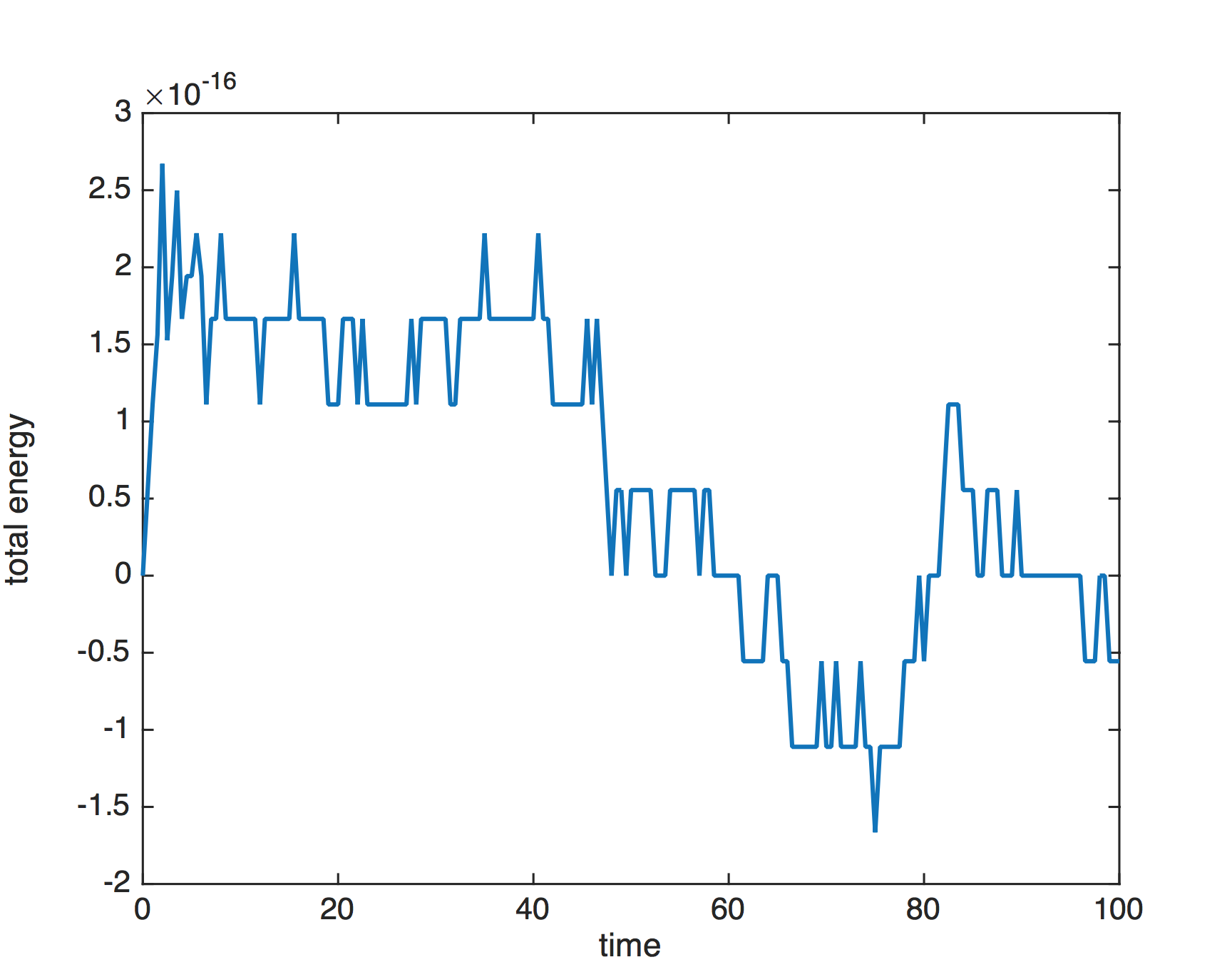
(b)

Figure 1: (a) Plot of the evolution of the discrete external power $A_{ext}$ (red), and the difference in the Hamiltonian $H(t_{n})-H(t_{0})$ (blue). (b) The sum of these two energies. Step size $h=0.5$.

IV-B Controlled Pendulum

For a second experiment consider the simple pendulum, with a small non-linear controller term for the momentum. The system has the format (II) with $x=[q,p]^{T}\in\mathbb{R}^{2}$ and

$$H(q,p) = \frac{1}{2}p^{2}+1-\cos q,$$

$$B(x) = J,$$

$$G(x) = [0,1]^{T},$$ (33)

$$u = \phi(y)=-0.01\arctan y.$$

Using the theory from Theorem II.4, one can show that this system will converge from almost every initial condition to the stable equilibrium $p=0$, $q=n2\pi$ for some integer $n$. Note that all these values of $q$ correspond to the same physical position. The system also has an unstable equilibrium at $p=0$, $q=(2n+1)\pi$.

In Fig. 2, 3, and 4 we compare the evolution of the position, the absolute error in the Hamiltonian, and the input $u$ respectively for method (25), the implicit midpoint method, the averaged vector field method, and the improved Euler method, all second order. The initial state is $x(0)=[2.8,1.4]^{T}$. We observe that the AVF method and the method (25) (which is based on this), outperforms the implicit midpoint, not to mention the improved Euler method, for the choice of step size, $h=0.5$.

In particular, in Fig. 2, the two latter methods give the wrong number of full rotations, $n$, of the pendulum before it starts to converge towards the stable equilibrium. Consequently the input signal as shown in Fig. 3 is also qualitatively wrong for these methods. In contrast, both the AVF method and the method (25) produce results which are difficult to distinguish from the exact solution on the scale shown. The AVF method and the method (25) are seen to have comparable energy preservation in Fig. 4, which is superior to the implicit midpoint and the improved Euler method.

Figure 2: Evolution of the pendulum angle $q$ for (33). Shown are the exact solution (Ex.), the method (25) (AVFPHS), the implicit midpoint method (IM), the averaged vector field method (AVF), and the improved Euler method (IE).

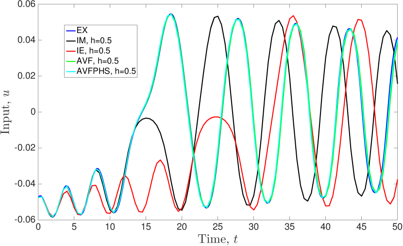
Figure 3: Evolution of the input $u$ for (33). Shown are the exact solution (Ex.), the method (25) (AVFPHS), the implicit midpoint method (IM), the averaged vector field method (AVF), and the improved Euler method (IE).

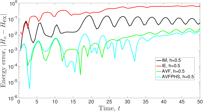
Figure 4: Evolution of the absolute error in the Hamiltonian for (33). Shown are the method (25) (AVFPHS), the implicit midpoint method (IM), the averaged vector field method (AVF), and the improved Euler method (IE).

IV-C Capacitor Microphone

For a system with dissipation, we consider the capacitor microphone from [28], which can also be written on the format (II) with $x=[q,p,Q]^{T}\in\mathbb{R}^{3}$ and

$$H(x) = \frac{1}{2m}p^{2}+\frac{1}{2}(q-\bar{q})^{2}+\frac{1}{2}qQ^{2},$$

$$B(x) = \left[\begin{array}[]{ccc}0&1&0\\ -1&-c&0\\ 0&0&-1/R\\ \end{array}\right],$$ (37)

$$G(x) = [0,1,1/R]^{T},$$ (38)

$$u = -\phi(y)=-\frac{1}{2}\sqrt[3]{y}.$$

Here $R=100$ is the resistance, and $c=0.1$ the damping constant of the spring to which the right capacitor plate, with mass $m=4$, is attached. $\bar{q}=3$ is the equilibrium point of the spring.

In Fig. 5 the evolution of the absolute error in the Hamiltonian for the dissipative system (38) is compared for method (25) and the improved Euler method, with step size $h=0.5$. Method (25) is again seen to better capture the correct evolution of the energy when compared to improved Euler. Results for the implicit midpoint method and the averaged vector field method were here comparable to method (25).

Figure 5: Evolution of the absolute error in the Hamiltonian $|H(x_{n})-H(x(t_{n})|$ for (38). Shown are the method (25) (AVFPHS), and the improved Euler method (IE).

V Conclusion

We have presented a systematic way to design discrete port-Hamiltonian systems, starting from a continuous system, by applying discrete gradient methods and splitting methods. The obtained discrete port-Hamiltonian systems are passive, and can be globally stabilized with respect to an equilibrium point by an appropriate choice of the input of the discrete system. The obtained discrete systems are port-Hamiltonian in the sense that they preserve a discrete notion of passivity and a generalized Dirac structure. The methods derived using this approach showed promising results in numerical experiments.

[Higher Order Discrete Gradient Methods] Generalisations of the second order method (25) to higher order can be obtained using a collocation idea as in [19]. Let us denote the Lagrange basis function on the node $c_{j}$ by $\ell_{j}$ for $j=1,\dots,s$, write $\sigma(t)$ for the collocation polynomial, and define $X_{\tau}:=\sigma(t_{n}+\tau h)$ and $X_{j}:=\sigma(t_{n}+c_{j}h)$. Now, consider the following collocation method to integrate (II):

$$\sigma(t_{n}) = x_{n},$$

$$\dot{\sigma}(t_{n}+c_{j}h) = B(X_{j})\bar{\nabla}H_{j}+G(X_{j})u_{j},$$ (39)

$$x_{n+1} = \sigma(t_{n}+h),$$

with

$$b_{j} := \int_{0}^{1}\ell_{j}(\alpha)\,d\alpha,$$

$$\bar{\nabla}H_{j} := \int_{0}^{1}\,\frac{\ell_{j}(\alpha)}{b_{j}}\,\nabla H(X_{\alpha})\,d\alpha,\ \ y_{j}:=G(X_{j})^{T}\bar{\nabla}H_{j},$$

and where the discrete controls $u_{j}$ depend on $\sigma$. Using Lagrange interpolation we can express the derivative of the collocation polynomial as

$$\dot{\sigma}(t_{n}+\tau h)=\sum_{j=1}^{s}\ell_{j}(\tau)\left[B(X_{j})\bar{\nabla}H_{j}+G(X_{j})u_{j}\right],$$

and obtain $X_{\tau}=\sigma(t_{n}+\tau h)$ by integration. We may define stage values for the output as

$$y_{j}=G(X_{j})^{T}\bar{\nabla}H_{j}.$$

The collocation polynomial $X_{\tau}$ gives a natural continuous form of the numerical solution on the whole interval of integration. Along the approximated solution $X_{\tau}$, a polynomial of degree $s$, we will show that the numerical method preserves a discrete passivity property, for quadratures $c_{1},\dots,c_{s}$ with positive weights $b_{1},\dots,b_{s}$.

In fact we have

$$H(x_{n+1})-H(x_{n})=h\int_{0}^{1}\nabla H(X_{\tau})^{T}\dot{\sigma}(t_{n}+\tau h)\,d\tau.$$

Then after simple calculations we obtain

$$H(x_{n+1})-H(x_{n}) = h\sum_{j=1}^{s}b_{j}\bar{\nabla}H_{j}^{T}B(X_{j})\bar{\nabla}H_{j}$$

$$+\>h\sum_{j=1}^{s}b_{j}\bar{\nabla}H_{j}^{T}G(X_{j})u_{j},$$

and upon using that $B(\cdot)$ is skew-symmetric

$$H(x_{n+1})-H(x_{n}) = h\sum_{j=1}^{s}b_{j}\bar{\nabla}H_{j}^{T}G(X_{j})u_{j}$$ (40)

$$= h\sum_{j=1}^{s}b_{j}y_{j}^{T}u_{j},$$

which clearly satisfies the discrete energy balance equation (21). The consequent passivity inequality becomes

$$H(x_{n+1})-H(x_{n})\leq h\sum_{j=1}^{s}b_{j}y_{j}^{T}u_{j}.$$

We now state and prove the following theorem

Theorem .1.

Assume that the discrete port-Hamiltonian system (39) defines a unique one step map $x_{n+1}=\Psi(x_{n})$, and that the system is passive with radially unbounded positive definite storage function $H$. Furthermore assume that no numerical solution $\{x_{n}\}_{n\in\mathbb{N}}$ satisfying the system of equations

$$\sigma(t_{n}) = x_{n},$$

$$\dot{\sigma}(t_{n}+c_{j}h) = B(X_{j})\bar{\nabla}H_{j},$$ (41)

$$x_{n+1} = \sigma(t_{n}+h),$$

can simultaneously satisfy the requirement $y_{j}=0$ for $j=1,\dots,s$ at every solution step, other than the trivial solution, i.e. $x_{n}=0$ for $n\in\mathbb{N}$. Then the origin $x=0$ can be globally stabilised with the choice of an appropriate control input $u_{j}=-\phi(y_{j})$ where $\phi$ is a function such that $\phi(0)=0$ and $y^{T}\phi(y)>0$ for all $y\neq 0$.

Proof.

From (40) we have

$$\Delta H(x_{n}) = H(\Psi(x_{n}))-H(x_{n})$$

$$= -h\sum_{j=1}^{s}b_{j}\bar{\nabla}H_{j}^{T}G(X_{j})\phi(G(X_{j})^{T}\bar{\nabla}H_{j})\leq 0,$$

where the last inequality follows from the weights $b_{j}$ being positive and the properties of $\phi$. Note that this inequality holds termwise. Since $H$ is continuous on $\mathbb{R}^{n}$ it is a (discrete) Lyapunov function for (39) on $\mathbb{R}^{n}$. In addition, because $H$ is radially unbounded, it follows that all solutions of this discrete system are bounded.

Consequently from Proposition III.1, $x_{n}\rightarrow M\neq\emptyset$, where $M$ is the largest positively invariant set contained in the set $E=\{x\in\mathbb{R}^{n}:\Delta H(x)=0\}$. Thus if $M=\{0\}$ the origin will be globally asymptotically stable.

Now, from the above calculations $\Delta H(x_{n})=0$ implies $y_{j}=0$ for all $j$, which from the properties of $\phi$ implies that $u_{j}=0$ for all $j$. Therefore (39) reduces to (41). Now from the zero-state observability requirement $x_{n}=0$ for $n\in\mathbb{N}$, and consequently $M=\{0\}$. ∎

Elena Celledoni Biography will be included in the final published version, if the paper is accepted.

Eirik Hoel Høiseth Biography will be included in the final published version, if the paper is accepted.

References

• [1] H. M. Paynter, Analysis and design of engineering systems.   The MIT Press, Cambridge, Massachusetts, 1960.
• [2] A. Bloch, J. Baillieul, P. Crouch, and J. Marsden, Nonholonomic mechanics and control, ser. Interdisciplinary applied mathematics.   New York: Springer-Verlag, 2003.
• [3] J. Marsden and T. Ratiu, Introduction to mechanics and symmetry, 2nd ed.   Springer-Verlag New York, 1999, vol. 17.
• [4] R. Abraham and J. Marsden, Foundation of Mechanics, 2nd ed.   Addison Wesley, 1978.
• [5] A. Weinstein, “The local structure of Poisson manifolds,” J. Differential Geom., vol. 18, no. 3, pp. 523–557, 1983.
• [6] A. van der Schaft and B. Maschke, “The Hamiltonian formulation of energy conserving physical systems with external ports,” AEU - Archiv für Elektronik und Übertragungstechnik, vol. 49, no. 5-6, pp. 362–371, 1995.
• [7] M. Dalsmo and A. van der Schaft, “On representations and integrability of mathematical structures in energy-conserving physical systems,” SIAM J. Control and Optimization, vol. 37, no. 1, pp. 54–91, 1998. [Online]. Available: http://dx.doi.org/10.1137/S0363012996312039
• [8] A. van der Schaft and D. Jeltsema, “Port-Hamiltonian systems theory: An introductory overview,” Foundations and Trends in Systems and Control, vol. 1, no. 2-3, pp. 173–378, 2014. [Online]. Available: http://dx.doi.org/10.1561/2600000002
• [9] R. Ortega, A. J. van der Schaft, and B. M. Maschke, Stabilization of port-controlled Hamiltonian systems via energy balancing, ser. Lecture Notes in Control and Information Sciences.   London: Springer London, 1999, vol. 246, pp. 239–260. [Online]. Available: http://dx.doi.org/10.1007/1-84628-577-1-13
• [10] E. Hairer, C. Lubich, and G. Wanner, Geometric numerical integration, Structure-preserving algorithms for ordinary differential equations, ser. Springer Series in Computational Mathematics.   Springer, Heidelberg, 2010, vol. 31, reprint of the second (2006) ed.
• [11] R. de Vogelaere, “Methods of integration which preserve the contact transformation property of the Hamiltonian equations,” Tech Report, Dept. Math., Univ. of Notre Dame, no. 4, 1956.
• [12] R. D. Ruth, “A Canonical Integration Technique,” IEEE Transactions on Nuclear Science, vol. 30, pp. 2669–2671, 1983.
• [13] K. Feng, “On difference schemes and symplectic geometry,” Proceedings of the 5-th Intern. Symposium on differential geometry & differential equations, August 1984, Beijing, pp. 42–58, 1985.
• [14] J. M. Sanz-Serna and M. P. Calvo, Numerical Hamiltonian problems, 1st ed.   Chapman & Hall, London ; New York, 1994.
• [15] J. E. Marsden and M. West, “Discrete mechanics and variational integrators,” Acta Numer., vol. 10, pp. 357–514, 2001. [Online]. Available: http://dx.doi.org/10.1017/S096249290100006X
• [16] O. Gonzalez, “Time integration and discrete Hamiltonian systems,” J. Nonlinear Sci., vol. 6, no. 5, pp. 449–467, 1996. [Online]. Available: http://dx.doi.org/10.1007/s003329900018
• [17] G. R. W. Quispel and G. S. Turner, “Discrete gradient methods for solving ODEs numerically while preserving a first integral,” J. Phys. A, vol. 29, no. 13, pp. L341–L349, 1996. [Online]. Available: http://dx.doi.org/10.1088/0305-4470/29/13/006
• [18] G. R. W. Quispel and D. I. McLaren, “A new class of energy-preserving numerical integration methods,” J. Phys. A, vol. 41, no. 4, p. 045206, 2008. [Online]. Available: http://stacks.iop.org/1751-8121/41/i=4/a=045206
• [19] D. Cohen and E. Hairer, “Linear energy-preserving integrators for Poisson systems,” BIT Numer Math, vol. 51, pp. 91–101, 2011.
• [20] E. Celledoni, E. Høiseth, and N. Ramzina, “Passivity-preserving splitting methods for controlled, input-output passive rigid body systems,” preprint on webpage at arxiv.org/abs/1408.2544.
• [21] H. Khalil, Nonlinear Systems, 3rd ed., ser. Pearson Education.   Prentice Hall, 2002.
• [22] O. Egeland and J. T. Gravdahl, Modeling and Simulation for Automatic Control.   Marine Cybernetics, Trondheim, 2002, corrected second printing 2003. [Online]. Available: https://books.google.no/books?id=oK0VAAAACAAJ
• [23] R. Ortega, A. Loría, P. J. Nicklasson, and H. Sira-Ramírez, Passivity-based Control of Euler- Lagrange Systems, ser. Communications and Control Engineering.   Springer London, 1998. [Online]. Available: http://dx.doi.org/10.1007/978-1-4471-3603-3
• [24] S. Aues, D. Eberard, and W. Marquis-Favre, “Canonical interconnection of discrete linear port-Hamiltonian systems,” IEEE Conference on Decision and Control, vol. 52, pp. 3166–3171, 2013. [Online]. Available: http://dx.doi.org/10.1109/CDC.2013.6760366
• [25] J. LaSalle, The Stability and Control of Discrete Processes, ser. Applied Mathematical Sciences.   Springer New York, 1986, vol. 62. [Online]. Available: http://dx.doi.org/10.1007/978-1-4612-1076-4
• [26] S. Blanes and F. Casas, “On the necessity of negative coefficients for operator splitting schemes of order higher than two,” Applied Numerical Mathematics, vol. 54, no. 1, pp. 23 – 37, 2005. [Online]. Available: http://dx.doi.org/10.1016/j.apnum.2004.10.005
• [27] E. Celledoni, R. I. McLachlan, D. I. McLaren, B. Owren, G. R. W. Quispel, and W. M. Wright, “Energy-preserving Runge-Kutta methods,” ESAIM: M2AN, vol. 43, no. 4, pp. 645–649, 2009. [Online]. Available: http://dx.doi.org/10.1051/m2an/2009020
• [28] A. van der Schaft, L2-Gain and Passivity Techniques in Nonlinear Control, 3rd ed., ser. Communications and Control Engineering.   Springer International Publishing, 2017, originally published as Volume 218 in the series: Lecture Notes in Control and Information Sciences. [Online]. Available: http://dx.doi.org/10.1007/978-3-319-49992-5