Detection of radio emission from the gamma-ray pulsar J1732$-$3131 at 327 MHz

Abstract

Although originally discovered as a radio-quiet gamma-ray pulsar, J1732$-$3131 has exhibited intriguing detections at decameter wavelengths. We report an extensive follow-up of the pulsar at 327 MHz with the Ooty radio telescope. Using the previously observed radio characteristics, and with an effective integration time of 60 hrs, we present a detection of the pulsar at a confidence level of 99.82$\%$. The 327 MHz mean flux density is estimated to be 0.5$-$0.8 mJy, which establishes the pulsar to be a steep spectrum source and one of the least luminous pulsars known to date. We also phase-aligned the radio and gamma-ray profiles of the pulsar, and measured the phase-offset between the main peaks in the two profiles to be 0.24$\pm$0.06. We discuss the observed phase-offset in the context of various trends exhibited by the radio-loud gamma-ray pulsar population, and suggest that the gamma-ray emission from J1732$-$3131 is best explained by outer magnetosphere models. Details of our analysis leading to the pulsar detection, and measurements of various parameters and their implications relevant to the pulsar’s emission mechanism are presented.

1 Introduction

The number of gamma-ray pulsars detected by the large area telescope (LAT) on-board Fermi satellite has gone much beyond the most optimistic guesses published prior to its launch. This revolution in the population of gamma-ray pulsars is also well reflected by a very significant increase in the number of radio-quiet gamma-ray pulsars (35 so far; Caraveo, 2014). Given the statistically significant numbers of radio-quiet and radio-loud pulsars and their sensitive follow-ups at radio-frequencies, models predicting the gamma-ray emission regions in the outer magnetosphere are favored against those supporting the emission sites to be near the polar cap.

J1732$-$3131 is one of the LAT-discovered pulsars, with a rotation period of about 196 ms (see Table 1 for some other parameters of the pulsar). The early radio searches for its counterpart at high radio frequency (1374 MHz; Ray et al., 2011) turned out to be unsuccessful. However, searches at decameter wavelengths resulted in an intriguing detection of a faint signal at the expected period of the pulsar at a dispersion measure (DM) of 15.44$\pm$0.32 pc cm^-3(Maan et al., 2012, hereafter Paper I). The pulsar was detected in only one of the several observing sessions, indicating the sporadic nature of the radio emission. Detection of several mildly bright single pulses in the same observing session, at a DM consistent with that of the periodic signal, further substantiated the findings and suggested the pulsar to be active at radio frequencies (Paper I). Subsequent deep search at 34 MHz also resulted in evidences of very faint periodic signal from the pulsar, and provided more robust estimate of the flux density (Maan & Aswathappa, 2014, hereafter Paper II).

Table 1: Measured and derived parameters of PSR J1732-3131 (from ; ; , and this work).

Right Ascension, R.A.(J2000)		17:32:33.54	Dispersion Measure, DM(pc/cc)		$15.44\pm 0.32$
Declination, Dec. (J2000)		-31:31:23.0	Distance (kpc)		$0.60\pm 0.15$
Pulse Frequency, $\nu$ ($s^{-1}$)		5.08794112	Flux density at 327 MHz (mJy)		0.5$-$0.8
Frequency first derivative, $\dot{\nu}$ ($s^{-2}$)		-7.2609$\times 10^{-13}$	Spectral index		$-3.0$ to $-2.4$
Epoch of frequency (MJD)		54933.00	pseudo-luminosity at 1400 MHz ($\mu$Jy kpc2)		2.2$-$8.9

A likely explanation for the apparent lack of radio emission from the radio-quiet pulsars is that their narrow radio beams miss the sightline towards Earth (Brazier & Johnston, 1999; Watters & Romani, 2011). Since the radio emission beam is expected to become larger at low frequencies (radius-to-frequency mapping; Cordes, 1978), probability of our line-of-sight passing through the beam also increases. If the above detections of J1732$-$3131 at very low frequencies were indeed due to this fact, the pulsar can be expected to be a steep spectrum source. Detections at 34 MHz, when combined with non-detections at high radio frequencies, imply the spectral index to be steeper than $-2.3$. Deep observations of the pulsar at frequencies above 100 MHz could provide a reasonable estimate of the spectral index, and might even shed some light on its viewing geometry.

Since sky position of J1732$-$3131 is close to the centre of the Galaxy, the earlier high frequency radio searches would have suffered a loss in sensitivity due to the enhanced system temperature (T_sys). The upper limit on 1374 MHz flux density of the pulsar is 59 $\mu$Jy (Ray et al., 2011). For comparison, the L-band flux densities of the LAT-discovered pulsars J0106+4855 and J1907+0602 are only 8 and 3 $\mu$Jy, respectively (Pletsch et al., 2012; Abdo et al., 2010). Hence, flux density of J1732$-$3131 at higher radio frequencies might still be well within the range of already detected pulsars, and a deep integration could compensate for the high T_sys and help in detection.

Significant variability in the radio flux density of pulsars, at a range of timescales (from a single rotation period to several hundreds of seconds, or even larger), is well known. In the absence of a good understanding of possible radio emission from the radio-quiet gamma-ray pulsars, their extensive radio follow-ups might also be revealing. Recent detections of several energetic radio bursts from the Geminga pulsar (Maan, 2015) demonstrates the possible rewards of an extensive follow-up. The first radio detection of J1732$-$3131 (Paper I) suggested the presence of occasional bursty emission from the pulsar. This provides a strong motivation for a dedicated follow-up.

With the motivations stated above, we conducted deep observations of J1732$-$3131 using the Ooty radio telescope (ORT). Details of these observations and data processing are given in Section 2, followed by a detailed discussion on the results in Section 3. A summary of our findings is given in Section 4.

2 Observations and Data Processing

2.1 Observations and pre-search processing

Observations were conducted using the ORT situated in southern India (Swarup et al., 1971). The telescope is equatorially mounted, and has an offset parabolic cylindrical reflector with dimensions of 530 m and 30 m in north-south and east-west directions, respectively. With the mechanical steering in the east-west direction, sources can be tracked continuously for approximately 9 hours. In the north-south direction, the telescope beam is steered electronically to point at different declinations (DEC).

Extensive observations of J1732$-$3131 were carried out in March 2014 and April 2015. In March 2014, the source was observed for a total of 70.5 hours, distributed over 36 sessions. Typically, 2 observing sessions were conducted on every day. In April 2015, 37 observing sessions were conducted, amounting to a total of 54.5 hours of observing time. Each observing session was accompanied by a few minutes observation of a nearby strong pulsar, B1749$-$28, which was used as a control source. During each of the individual observing sessions, data were recorded in filterbank format, with 1024 channels across 16 MHz bandwidth centered at 326.5 MHz, with a time resolution of 0.512 ms, using the new pulsar receiver (Naidu et al., 2015). For simplicity, we refer the centre frequency as 327 MHz in the rest of the paper.

The filterbank data were used to identify the parts of data contaminated by radio frequency interference (RFI). The identification procedure involves computation of robust mean and standard deviation, and comparing the data with a specified threshold separately in the time and frequency domains. More details of this procedure can be found in Maan (2015) and Paper II. The RFI-contaminated time samples as well as spectral channels are excluded from any further processing.

2.2 Search procedures

The data were searched for transient as well as periodic signals from the pulsar. Briefly, the search for transient signals involves dedispersing the filterbank data for a number of optimally spaced trial DMs within the range 0$-$50 pc cm^-3, computing smoothed versions of each of the dedispersed timeseries for a number of trial pulse-widths, and searching for events above a specified threshold.

The filterbank data from individual sessions were searched for any dispersed signal at the expected rotation period of J1732$-$3131. Since the rotation ephemeris is known from timing of the gamma-ray data, periodic radio flux from the pulsar can be probed deeply by combining data from multiple sessions. Deep search for periodic emission from the pulsar involves folding the individual session filterbank data over the rotation period, adding the folded filterbank data from all the sessions in phase, and searching for a dispersed signal. Detailed descriptions of our single pulse as well as periodicity searches can be found in Paper II and Maan (2014).

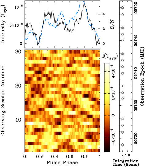
Figure 1: Individual rows in the colour image show phase-aligned 327 MHz average profiles of J1732$-$3131 obtained from different sessions (arranged in ascending order of observing epoch). The upper panel displays the net average profile (solid line) and the average profile from the earlier detection at 34 MHz (dotted line; see Paper I), for ready comparison. The intensity range of the 34 MHz profile is normalized to that of the 327 MHz profile. The 327 MHz intensity is plotted in units of T_sys, which is estimated to be 760 K towards the pulsar (see Section 3.4). All the individual profiles are smoothed by a 30° ($\sim 0.08$ in normalized pulse-phase) wide window. For the sessions corresponding to different rows in the image panel, the right panel shows the epochs of observation and the effective integration time (earliest epoch corresponds to first observing session).

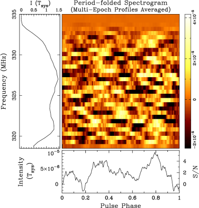
Figure 2: The color image shows dedispersed, period-folded and multi-epoch averaged 32-channel spectrogram of J1732$-$3131. The left and the bottom panels show the average spectrum and the net average profile, respectively, plotted in units of T_sys. As in Figure 1, all the profiles are smoothed by a 30^∘ wide window.

3 Results and Discussion

Our searches for bright dispersed pulses and periodic signal using data from individual observing sessions did not result in any significant detection above a signal-to-noise ratio (S/N) threshold of 8$\sigma$. More details of the deep searches using data from March 2014 and April 2015 are discussed below separately.

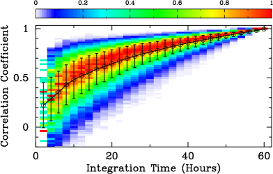
Figure 3: Each column in the colour-image shows the distribution function of normalized cross-correlation coefficient between partial average profiles corresponding to the integration time on horizontal axis and the net average profile. Peaks of all the distribution functions are normalized to 1. The ‘open circles’ connected by the continuous black line show the median correlation coefficient for each of the trial integration time. The errorbars on either side of the median correspond to the standard deviation measured from the distribution function.

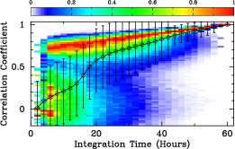
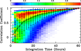
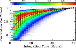
Figure 4: Same as in Figure 3 but now for simulated data (see text). The left, centre and right panels show results when randomly chosen 2, 4 and 8 of the 30 simulated profiles were modified to obtain the net average profile shape similar to that in upper panel of Figure 1.

3.1 Deep search using March 2014 data

Out of the 36 observing sessions conducted in 2014, 2 sessions were unusable due to severe contamination from RFI. In 4 other sessions, although typically less than 1% of the samples were identified as RFI-contaminated, data showed indications of faint RFI and abrupt jumps in power levels. To minimize effects of such systematics on the search sensitivity, data from all the above mentioned sessions were excluded from any further processing. To carry out deep search for a dispersed signal using data from the remaining 30 sessions, we used an up-to-date timing model of J1732$-$3131 obtained from the gamma-ray data (Kerr et al., 2015), to predict the pulsar’s rotation period and phase at different observing epochs using the pulsar timing software Tempo2. The deep search did not result in any significant signal above our detection threshold of 8$\sigma$.

To probe a possible underlying periodic signal fainter than our detection threshold, we dedispersed the data using a DM of 15.5 pc cm^-3  and computed average profiles for individual sessions. To compute the net average profile, the individual profiles were weighted and added coherently in the pulsar’s rotation phase. The weights for individual profiles were chosen to be directly proportional to the product of effective bandwidth and integration time, i.e., inversely proportional to the expected variance in the average profile. The 327 MHz net average profile integrated over an effective duration of 60 hours is shown in Figure 1 along with the average profiles from individual observing sessions. The net average profile exhibits a peak-to-peak S/N of nearly 6. For comparison, average profile of the pulsar at 34 MHz is overlaid on the net average profile in the upper panel. The two profiles are manually aligned, since the uncertainty in DM is not adequate enough to phase-align the profiles at such widely separated frequencies. A striking resemblance between the two profiles is clearly evident. Figure 2 shows the dedispersed and averaged spectrogram of all the data presented in Figure 1, and demonstrates that the faint periodic signal is uniformly present across the observing bandwidth.

3.1.1 Shape of the net average profile: a faint underlying signal or artifacts ?

Before we quantify the similarity between the average profiles at 327 and 34 MHz, it is important to assess whether the average profile shape has uniform contribution from all the sessions or dominated by artifacts in a single or a few individual profiles. A conventional way to test this is to examine the significance (e.g., peak S/N or reduced chi-square) of the average profile as data from successive sessions are integrated. Given the low S/N of the net average profile, we have used a bootstrap method to probe whether just a few sessions are affecting the average profile shape. For this purpose, we examine a correlation-based figure-of-merit (FoM) as a function of the integration time. Since the integration time for each of the individual average profiles is 2 hours, we have chosen the step between consecutive trial integration times in our bootstrap method also to be 2 hours. For each of the trial integration time, we randomly choose a sample of appropriate number of individual profiles, compute a partial average profile using this sample, and measure its cross-correlation coefficient with the net average profile as a FoM. Each bootstrap sample corresponding to a trial integration time consists of choosing $10^{4}$ non-redundant sample combinations of sessions using a reservoir sampling algorithm (Jeffrey, 1985), and computing the FoM for each of the combinations. This approach allows us to obtain a distribution of figures of merit for each of the trial integration time, with the median of the distribution assigned as the average FoM. For trial integration times involving less than 4 or more than 26 sessions, all the possible combinations of individual profiles are used to compute the FoM distribution.

The average FoM estimated from the above bootstrapping is shown in Figure 3 as a function of integration time, along with the colour-coded maps of corresponding distributions (histograms) with their peaks normalized to 1. The uniform distributions and smooth monotonic increase in the average FoM with the integration time is clearly evident, and strongly suggests that the shape of the net average profile shown in Figure 1 represents a faint signal consistently present in individual profiles obtained from different sessions.

To demonstrate how presence of artifacts in a few individual profiles would have reflected in the above analysis, we simulated 30 normally distributed noise profiles. The root-mean-square (rms) of the noise in these profiles was kept same as that of the observed profiles. Then a predecided number of profiles were modified in such a way that the average of all 30 profiles becomes similar to the net average profile in Figure 1. For this purpose, intensity of a scaled-version of the net average profile was randomly distributed between the selected profiles. The profiles to be modified were themselves chosen randomly. Figure 4 shows results of the bootstrapping analysis for three different cases when 2, 4 and 8 profiles were modified as mentioned above. The first two cases, i.e., when just 2 and 4 profiles are responsible for the average profile shape, result in glaringly different profile significance distributions. The third case starts approaching the uniform distributions and smooth increase in the average FoM for real data shown in Figure 3. However, minor differences are still noticeable, e.g., the average FoM rises much more sharply till integration times of about 20 hours. The results become nearly indistinguishable from Figure 3 when 16 profiles are modified (not shown but assessed separately). Hence, the shape of the net average profile is contributed by a significant number of sessions, perhaps all, and certainly not only by just a few.

Figure 5: The continuous and dashed lines show the peak S/N and the peak-to-peak S/N of the net average profile as a function of trial DM.

3.1.2 The net average profile: association with the pulsar

The 327 and 34 MHz profiles shown in the upper panel of Figure 1 exhibit striking resemblance, and both are consistent with each other within the noise uncertainties. As a quantitative measure of the similarity, the normalized cross-correlation coefficient between the two profiles is estimated to be 0.72.

To estimate the chance probability of obtaining a net average profile with the observed peak-to-peak S/N of nearly 6 and exhibiting striking similarity with the 34 MHz profile, we performed Monte-Carlo (MC) simulations. Each individual realization in our MC simulation involves generating 30 random (normal distribution) noise profiles, computing an average noise profile from these, and cross-correlating the average profile with the 34 MHz profile. To be compatible with the profiles shown in Figure 1, each of the random noise profiles is also smoothed with a $30\degr$ ($\sim 0.08$ in normalized pulse-phase) wide window. The resultant average noise profile is cross-correlated with the 34 MHz profile at all possible phase-shifts to determine the maximum normalized correlation coefficient. The maximum correlation coefficient and the peak-to-peak S/N of the average noise profile are noted down. From simulations of 1 million ($10^{6}$) such independent realizations, only $0.18\%$ times the average noise profile was found to be having peak-to-peak S/N more than 5.5 as well as the maximum correlation coefficient $\geq 0.72$. Hence, the probability of obtaining the 327 MHz profile with its measured significance and similarity to the 34 MHz profile just by chance is only 0.0018. In other words, the 327 MHz profile is consistent with being originated from the same source as the 34 MHz profile at a confidence level of $99.82\%$.

The confidence gained from the above MC simulations also motivates to explore the profile significance as a function of DM. Variation in the profile significance in terms of the peak S/N as well as peak-to-peak S/N with DM, obtained from our deep search methodology mentioned earlier, are shown in Figure 5. The profiles corresponding to the individual trial DMs were smoothed by a 30° wide window before computing the significance. Although the significance is low, peak S/N as well as peak-to-peak S/N are suggestive of a nominal DM of $16\pm 7$ pc cm^-3  which is consistent with DM estimated from the original detection, and provides an independent support for the low-significance net average profile to be originated from the pulsar.

3.2 Deep search using April 2015 data

Compared to the 2014 observations, data from the observing sessions conducted in 2015 showed overall more occurrences of RFIs. Strong RFIs and visible system artifacts made data from 8 observing sessions unusable, while those from 3 other sessions showed hints of low-level RFIs, and hence excluded from further processing. Deep search for the periodic signal from the pulsar using data from the remaining 26 sessions, amounting to a total of about 39 hours of integration time, did not result in any significant candidate above our detection threshold of $8\sigma$.

Following the procedure detailed in Section 3.1, we used the data from above 26 sessions to compute the net average profile dedispersed at 15.5 pc cm^-3. Note that the integration time for this profile is about 39 hours, as against 60 hours for the profile shown in Figure 1. Furthermore, sensitivity of the telescope during these observations was lower by a factor of 1.2$-$1.3, compared to that during the 2014 observations. Due to these factors, the peak-to-peak S/N of the average profile obtained from 2015 observations barely reaches 3.5$-$4. The average profiles can also be added in-phase to those from 2014 observations to achieve effectively a larger integration time. However, due to poorer sensitivity of the telescope during these observations, the effective increase in the integration time will be about 23–27 hours, which translates to only about 1$\sigma$ increase in the profile significance. Even this feeble enhancement is subjective to quality of the data being added, such as being free from any underlying faint RFIs. The 2015 data are found to be of overall poorer quality than the 2014 data. In any case, combining the observations from the two years did not improve the 2014 average profile by any significant amount.

3.3 Search for continuum emission

Given the large pulse duty cycle, and possible emission at all pulse phases, the pulsar might be better suited to be detected as a source of continuous emission using interferometric observations. With this motivation, we used GMRT archival data at 330 MHz, from nearly 4 hours long observations conducted in March 2004 (proposal code: 05SBA01) towards a nearby source G355.5+00. The rms noise obtained at the centre of the field is 0.6 mJy/beam. However, the pulsar is 61^′ away from the pointing centre, and the primary beam corrected rms noise at the location of the pulsar is about 3.4 mJy/beam. No source could be seen within 5^′ of the position of the pulsar (17h32m33.54s, $-$31d31^′23^′′; J2000). Therefore, we put a $3\sigma$ continuous emission upper limit of 10 mJy from the pulsar.

3.4 Flux density and spectral index estimates

To estimate the sky background temperature towards the pulsar, we used a low frequency sky map generating program, LFmap, to construct a sky map at 326.5 MHz. LFmap scales the 408 MHz all-sky map of Haslam et al. (1982) to the desired low frequency, taking into account the CMB, isotropic emission from unresolved extra-galactic sources, and the anisotropic Galactic emission. By computing a weighted average of the 326.5 MHz map at several points across the beam, using the following theoretical beam-gain pattern:
$P(RA,DEC)=\operatorname{sinc}^{2}{\left(\frac{b\,\sin{(RA)}}{\lambda}\right)}\times\operatorname{sinc}^{2}{\left(\frac{a\,\sin{(DEC)}}{\lambda}\right)}$,
where $a=\cos{(DEC)}\times 530$ m, $b=30$ m and $\lambda=0.92$ m, the sky background temperature towards the pulsar is estimated to be 610 K. Assuming an effective bandwidth of 13.6 MHz (85% of the total bandwidth), 50% pulse duty cycle, receiver temperature of 150 K, and an effective collecting area of 7500 m² (55% of physical area projected towards the pulsar), we estimate the pulsar’s average flux density to be in the range 0.5$-$0.8 mJy (for profile-S/N to be in the range 3$-$5 achieved from 60 hours of integration; Figure 1).

The above flux density estimate when combined with that at 34 MHz (Paper II) and assuming no turn-over in the spectrum, suggests the spectral index of the pulsar to be in the range $-2.4$ to $-3.0$. This range is consistent with the spectral index upper limit of $-2.3$ suggested in Paper II. We would like to emphasize that the above spectral index estimate will remain unaffected even if the actual pulse duty cycle happens to be different from what we have assumed. This is due to the fact that the profile widths are similar at 34 and 327 MHz (see Figure 1), and same pulse duty cycle (50%) has been assumed for estimating the flux densities at both the frequencies.

The continuum emission upper limit at 330 MHz presented in the previous subsection is consistent with the flux density of the pulsar estimated above. Recently, Frail et al. (2016) have reported a 3$\sigma$ flux density upper limit of 24 mJy/beam towards this pulsar at 150 MHz. Assuming no turn-over in the spectrum, the spectral index deduced above predicts a flux density of 3$-$8 mJy at 150 MHz, consistent with the result from Frail et al. (2016).

The steep spectrum index suggests the pulsar’s flux density at 1400 MHz to be 6$-$24 $\mu$Jy, consistent with the upper limit from earlier searches (Ray et al., 2011). The flux density is also comparable to that of the other two very faint pulsars mentioned in Section 1 (J0106+4855 and J1907+0602). However, J1732$-$3131 is relatively nearby implying a lower luminosity. Indeed the 1400 MHz pseudo-luminosity of the pulsar is only 2.2$-$8.9 $\mu$Jy kpc². If we use the NE2001 electron density model (Cordes & Lazio, 2002) to derive distance from DM, then the above range suggests J1732$-$3131 to be the least luminous among all the pulsars for which 1400 MHz flux density estimates are known (ATNF pulsar catalog; Manchester et al., 2005)! Even if we use the more recent electron density model by Yao et al. (2017), only a few pulsars have pseudo-luminosity less than that of J1732$-$3131. Hence, J1732$-$3131 is one of the least luminous radio pulsars known to date !

3.5 Profile morphology and implications to viewing geometry and emission mechanism

At this stage, we can perhaps review whether the 34 MHz detection of the pulsar was indeed benefitted by its correspondingly larger emission beam at low frequency. While strong constraints on the viewing geometry can be obtained only from polarization data, we can seek hints from the profile morphology and the radio spectrum. A grazing line of sight would tend to miss the high frequency radio emission beam and give rise to a steep spectrum (e.g., B0943+10 has a spectral index of -2.9; Malofeev et al., 2000). The mean spectral index for normal pulsars has been estimated to be $-1.4\pm 1.0$ (Bates et al., 2013). With the spectral index in the range $-2.4$ to $-3.0$, radio spectrum of J1732$-$3131 is indeed on the steeper side. However, more than 10% of the pulsars with characterized radio spectra have spectral indices in the range deduced for J1732$-$3131 (ATNF pulsar catalog), suggesting that the present constraints are too loose to be interpreted in the present context.

A grazing sight line would also imply a significant evolution of pulse-width and/or number of pulse components with frequency. The similarity of J1732$-$3131’s pulse profiles at frequencies separated by a factor of nearly 10 (at 34 and 327 MHz; Figure 1), suggests that there is no major evolution of the profile in this frequency range. However, minor evolution that is hindered by very low-S/N in both the profiles can not be excluded. Hence, the current data do not present a strong support for a favorable viewing geometry to be responsible for the pulsar’s original detection at low frequency.

The radio and gamma-ray profiles of the pulsar appear to have similar morphology (see Figure 4 of Paper I). Profile morphology and phase-alignment of the radio and gamma-ray profiles could give important clues about the location of the emission sites. The propagation of radio signals through the dispersive ISM introduces a delay $\Delta t\propto{\rm DM}\times\nu^{-2}$. The uncertainty in DM from the original detection (15.44$\pm$0.32  pc cm^-3) was not adequate enough to probe the phase-alignment of the 34 MHz profile with its gamma-ray counterpart. However, at 327 MHz an uncertainty in DM as large as 0.3  pc cm^-3 translates to a delay equivalent to only about 0.06 of the pulsar’s rotation period, allowing us to examine the phase-alignment between the radio and the gamma-ray profiles.

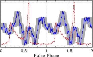
Figure 6: Phase-aligned radio and gamma-ray profiles of J1732$-$3131. The continuous blue line shows the 327 MHz average profile from 2014 observations and the dashed-dotted-dashed red curve shows the gamma-ray profile. The horizontal extent of the grey shade on either side of the radio profile indicates the uncertainty in phase corresponding to 1$\sigma$ error in DM. For clarity, both the profiles are duplicated and plotted over a range spanning two rotations of the pulsar.

The dispersive delay ($\Delta t$) as well as delays associated with the configuration of the telescope relative to the solar system barycenter, are accounted for by Tempo2 while predicting the pulsar’s phase at a given observing epoch. The instrumental delay associated with the ORT was estimated by fitting a ‘jump’ in pulse arrival times of a known fast pulsar obtained at ORT and GMRT using Tempo2. The delay was confirmed by independent tests, and was taken in to account by modifying the recorded start time of the individual observations appropriately. The gamma-ray photon arrival times are converted to the geocenter to remove the effects of the Fermi LAT spacecraft motion around the earth. The corrected arrival times are then used with Tempo2 in predictive mode to compute an average profile. To probe the phase-alignment of the radio and gamma-ray light curves, we compute the arrival time correction from the geocenter to the ORT as well as the associated phase-correction. We use these corrections to convert the gamma-ray light curve to the ORT, and compare it with the radio profile observed at the site. We successfully tested our procedure by reproducing the known phase offset of 0.44 between the radio and gamma-ray profiles of the pulsar J0437$-$4715 (Abdo et al., 2013).

The phase-aligned radio and gamma-ray profiles of J1732$-$3131 are plotted in Figure 6. The lag ($\delta$) of the main peak in the gamma-ray profile with respect to the highest peak in the radio profile is $0.24\pm 0.06$ in pulse-phase. Note that the the uncertainty of 0.06 is entirely due to that in DM, and any contribution from the statistical uncertainty on the position of the peaks is much smaller.

For majority of young gamma-ray pulsars, the phase difference between the leading and trailing peaks in gamma-ray profile ($\Delta$) has been found to be anti-correlated with $\delta$. This relationship between $\Delta$ and $\delta$ was initially shown by Romani & Yadigaroglu (1995) to be a general property of the outer-magnetosphere models with caustic pulses. Majority of the young and middle-aged gamma-ray pulsars detected by Fermi LAT have confirmed to the $\Delta-\delta$ relationship (Abdo et al., 2013). More recently, Pierbattista et al. (2016) have constrained several $\gamma$-ray geometrical models by comparing simulated and observed light curve morphological characteristics, including the correlation of $\delta$ with other observable quantities. Assuming a vacuum-retarded dipole magnetic field, they show that the Outer Gap (OG) model (Cheng et al., 2000) and the One Pole Caustic (OPC) model (an alternative formulation of the OG; Romani & Watters, 2010) best explain the trends between various observed and deduced parameters. Our deduced value of $\delta=0.24\pm 0.06$ suggests that J1732$-$3131 also follows the common trends (like correlation of $\delta$ with rotation period and $\Delta$) exhibited by a large fraction of radio-loud gamma-ray pulsars ($\Delta=0.42$, and see, for example, Figures 12 and 13 in Pierbattista et al., 2016). Hence, following the conclusions of Pierbattista et al. (2016), the observed radio and gamma-ray light curves of J1732$-$3131 are also best explained by the OG and OPC models.

4 Summary

In the previous sections, we have presented details of our extensive observations, and deep search for periodic signal from the gamma-ray pulsar J1732$-$3131 at 327 MHz using the Ooty radio telescope. Despite the high background sky temperature, our deep integration allowed us to probe very faint periodic signal from the pulsar. Using nearly 60 hours of observations conducted in March 2014, we have presented detection of periodic signal at a DM of 15.5 pc cm^-3  from the pulsar at a confidence level of 99.82%. We estimate the 327 MHz flux density of the pulsar to be 0.5$-$0.8 mJy, and the spectral index in the range from $-2.4$ to $-3.0$. The 1400 MHz pseudo-luminosity of the pulsar is only 2.2$-$8.9 $\mu$Jy kpc², and suggests the pulsar to be one of the least luminous pulsars known to date! We also phase-aligned the radio and gamma-ray profiles, and measured the phase-offset between the main peaks in the two profiles to be $0.24\pm 0.06$. This non-zero phase-lag favors the models wherein the gamma-ray emission originates in the outer magnetosphere of the pulsar.

J1732$-$3131 was detected during a rare enhancement in its flux density, most likely due to scintillation (Paper I). Subsequent detections of the pulsar using deep follow-up observations ( Paper II, and this work) have been possible only since its DM was known from the first detection (Paper I). So, it is possible that some of the radio-quiet gamma-ray pulsars might actually be very faint radio sources, and hence not detected in the radio searches using current generation telescopes. The high sensitivity of upcoming radio telescopes like square kilometre array (SKA) and the five hundred meter aperture spherical telescope (FAST) will enable radio detection, and facilitate better studies of such pulsars.

References

- Abdo et al. (2010) Abdo A. A., et al., 2010, ApJ, 711, 64
- Abdo et al. (2013) Abdo A. A., et al., 2013, ApJS, 208, 17
- Bates et al. (2013) Bates S. D., Lorimer D. R., Verbiest J. P. W., 2013, MNRAS, 431, 1352
- Brazier & Johnston (1999) Brazier K. T. S., Johnston S., 1999, MNRAS, 305, 671
- Caraveo (2014) Caraveo P. A., 2014, ARA&A, 52, 211
- Cheng et al. (2000) Cheng K. S., Ruderman M., Zhang L., 2000, ApJ, 537, 964
- Cordes (1978) Cordes J. M., 1978, ApJ, 222, 1006
- Cordes & Lazio (2002) Cordes, J. M., & Lazio, T. J. W. 2002, arXiv:astro-ph/0207156
- Frail et al. (2016) Frail D. A., Jagannathan P., Mooley K. P., Intema H. T., 2016, ApJ, 829, 119
- Haslam et al. (1982) Haslam C. G. T., Salter C. J., Stoffel H., Wilson W. E., 1982, A&AS, 47, 1
- Jeffrey (1985) Jeffrey S. V., 1985, ACM Transactions on Mathematical Software (TOMS), 1, 37
- Kerr et al. (2015) Kerr M., Ray P. S., Johnston S., Shannon R. M., Camilo F., 2015, ApJ, 814, 128
- Maan (2014) Maan Y., 2014, PhD thesis, Indian Institute of Science, Bangalore, India
- Maan (2015) Maan Y., 2015, ApJ, 815, 126
- Maan & Aswathappa (2014) Maan Y., Aswathappa H. A., 2014, MNRAS, 445, 3221
- Maan et al. (2012) Maan Y., Aswathappa H. A., Deshpande A. A., 2012, MNRAS, 425, 2
- Malofeev et al. (2000) Malofeev V. M., Malov O. I., Shchegoleva N. V., 2000, Astron. Rep., 44, 436
- Manchester et al. (2005) Manchester R. N., Hobbs G. B., Teoh A., Hobbs M., 2005, AJ, 129, 1993
- Naidu et al. (2015) Naidu A., Joshi B. C., Manoharan P. K., Krishnakumar M. A., 2015, ExA, 39, 319
- Pierbattista et al. (2016) Pierbattista M., Harding A. K., Gonthier P. L., Grenier I. A., 2016, A&A, 588, A137
- Pletsch et al. (2012) Pletsch H. J., et al., 2012, ApJ, 744, 105
- Ray et al. (2011) Ray P. S., et al., 2011, ApJS, 194, 17
- Romani & Watters (2010) Romani R. W., Watters K. P., 2010, ApJ, 714, 810
- Romani & Yadigaroglu (1995) Romani R. W., Yadigaroglu I.-A., 1995, ApJ, 438, 314
- Swarup et al. (1971) Swarup G., et al., 1971, NPhS, 230, 185
- Watters & Romani (2011) Watters K. P., Romani R. W., 2011, ApJ, 727, 123
- Yao et al. (2017) Yao, J. M., Manchester, R. N., & Wang, N. 2017, ApJ, 835, 29