Multiband superconductivity in ${\rm BiS_{2}}$-based layered compounds

Abstract

A mean-field treatment is presented of a square lattice two-orbital-model for ${\rm BiS_{2}}$ taking into account intra- and inter-orbital superconductivity. A rich phase diagram involving both types of superconductivity is presented as a function of the ratio between the couplings of electrons in the same and different orbitals (${\rm\eta=V_{XX}/V_{XY}}$) and electron doping x. With the help of a quantity we call orbital-mixing ratio, denoted as $R(\phi)$, the phase diagram is analyzed using a simple and intuitive picture based on how $R(\phi)$ varies as electron doping increases. The predictive power of $R(\phi)$ suggests that it could be a useful tool in qualitatively (or even semi-quantitatively) analyzing multiband superconductivity in BCS-like superconductors.

1 Introduction

The study of two-band superconductivity (SC) [1, 2, 3] (or, more generally, multiband SC) has become of increasing relevance as superconducting materials with overlapping bands at the Fermi surface, like, for example, ${\rm MgB_{2}}$ [4, 5], are discovered. What distinguishes these systems from the more traditional single-band case is the coexistence, at the Fermi level, of electrons from different bands (originating from different orbitals). These electrons, which are directly involved in the superconducting ground state, can, in principle, pair in a variety of ways. The large class of multiband superconductors includes heavy-fermion systems [6, 7], the well-studied ${\rm MgB_{2}}$ [8], the pnictides [9] and, more recently, the layered sulfides ${\rm BiS_{2}}$ [10]. The types of pairing in multiband systems can be categorized in two main groups, namely intraband and interband pairing, depending on the predominant paring interaction in the system. These two types of pairings are not mutually exclusive, they may coexist and even ‘compete’ in the same material, changing in relative importance as some external parameter, as pressure or doping, is varied [11]. The superconducting state resulting from the addition of a second band [1, 12] to the traditional single-band BCS state [13] shows many interesting new features, like the possibility of formation of two superconducting gaps, which may then be observed by either Angle-Resolved Photoemission Spectroscopy (ARPES)[14], Scanning Tunneling Spectroscopy (STS) [15], or thermal transport measurements under magnetic field [6], for example; the possibility of pairing even when the electron-electron interaction in one of the bands is repulsive, in which case, when an interaction between the bands is introduced, $T_{c}$ increases in comparison to the single-band attractive case[1]. In addition, the isotope effect vanishes when the interband interaction is large, explaining the behavior of superconductors like ${\rm Nb_{3}Sn}$ [12]. Note that the motivation for Suhl et al. [1] to introduce the ‘extra’ band was to try and explain the (relatively) high-${\rm T_{c}}$ observed in transition metal superconducting compounds [16]. An indication that a second band had to be taken into account to treat SC in the transition metal elements was that s-d electron scattering seemed to be important to explain their resistivity in the normal state. Suhl et al. [1] analyzed three different situations (denoting the intraband pairing interactions as ${\rm V_{ss}}$ and ${\rm V_{dd}}$, and the interband as ${\rm V_{sd}}$): (i) finite ${\rm V_{sd}}$ and ${\rm V_{ss}=V_{dd}=0}$, obtaining two different gaps (unless the density of states $\rho_{s}=\rho_{d}$, in which case the gaps are equal) whose dependence on temperature is BCS-like, but that, nonetheless, have the same $T_{c}$; (ii) ${\rm V_{sd}=0}$, where there are two gaps as well, with a BCS-like temperature dependence, however, with two different $T_{c}$ values; and (iii) if a small ${\rm V_{sd}\ll\sqrt{V_{ss}V_{dd}}}$ is turned on, a single $T_{c}$ is obtained that is close but always above the larger $T_{c}$ in (ii), as well as a gap with a dependence on temperature that is an interpolation between the gaps obtained in (ii). Two clear examples of case (i) can be observed first in ${\rm MgB_{2}}$ trough STS data as a function of temperature [15], and second in the pnictide compound ${\rm Ba_{0.6}K_{0.4}Fe_{2}As_{2}}$ through ARPES [14].

In this work, using an orbital basis, we will study the contribution of different types of pairings, intra- and inter-orbital, to the superconducting phase of ${\rm BiS_{2}}$ systems as a function of electron doping. Reference [17], where 32 classes of superconductors were studied, placed the ${\rm BiS_{2}}$ family of superconductors in the ‘possibly unconventional’ column. Reference [18] describes the experiments that suggest the possibility of these materials exhibiting unconventional superconductivity. The fact that these results come from polycrystalline samples, which are prone to inhomogeneities and random orientation of crystallites (which becomes relevant for measurements depending on the application of a magnetic field) warrants the cautious approach taken by the community working on ${\rm BiS_{2}}$. Thus, in the present work, we do not assume any specific pairing mechanism, although we briefly refer to ‘phonon pair-scattering’, for the sake of argument, when discussing the results. As to the SC gap, muon-spin rotation ($\mu$SR) experiments [10], for example, support multiband SC in the ${\rm BiS_{2}}$-based layered compound ${\rm Bi_{4}O_{4}S_{3}}$, pointing to two s-wave-type energy gaps, although the authors do not rule out the possibility of fitting the data with a single s-wave gap. Therefore, we will consider these materials as s-wave ($\vec{k}$-independent) singlet superconductors and use a mean-field approach to analyze its double-gap properties. In general, interband pairing between bands which cross the Fermi surface at different wave-vectors may favor the appearance of inhomogeneous superconducting states characterized by a wave-vector Q corresponding to the difference between the different band wave-vectors [19, 20, 21]. No evidence of such phenomenon has been experimentally observed in ${\rm BiS_{2}}$ compounds, therefore we do not take this possibility into account in our model. Features associated with low dimensionality [22, 23, 24] are important to determine the electronic structure of these materials, but, close to the SC transition, fluctuations are averaged out as indicated by the large coherence length measured for these materials [25, 26], thus justifying the use of a BCS (mean-field) treatment of the problem, as undertaken here. Aside from the controversy regarding the pairing mechanism, superconductors based on ${\rm BiS_{2}}$ layers have revealed complex and surprising properties. For example, recently, coexistence of magnetism and SC has been reported [27] in ${\rm Bi_{4-x}Mn_{x}O_{4}S_{3}}$. These phenomena are observed in different layers of the system and appear as rather independent of each other. The substitution by Co and Ni instead of Mn suggests that the increase in $T_{c}$ due to the latter can be attributed to its mixed valence, which allows for an effective charge transfer to the superconducting layers.

This work is divided as follows: In section 2.1 we present the tight-binding two-orbital model for ${\rm BiS_{2}}$, showing in detail how does the Fermi surface changes with electron doping. Section 2.2 presents the pairing interactions we are considering, while section 2.3 develops the gap equations at the mean-field level. Section 2.4 closes with some simplifying assumptions regarding the paring interactions, which reduce the number of gap equations from 4 to 2. We close section II by presenting the solution to the gap equations as a function of ${\rm\eta=V_{XX}/V_{XY}}$ (the ratio of the relevant pairing couplings) and the electron doping x. In Section 3.1, we clearly define what is meant by orbital-mixing, by introducing the quantity $R(\phi)$ to measure it along the Fermi surface, and describe its relevance to multiband SC. Section 3.2 describes how the structures seen in both gap functions below the Lifshitz transition can be understood through the way $R(\phi)$ changes with doping. In section 3.3 the same is done above the Lifshitz transition. In addition, section 3.4 presents results for the superconducting critical temperature $T_{c}$, which are qualitatively in agreement with those for ${\rm BiS_{2}}$ compounds. The paper closes with section 4, where Summary and Conclusions are given.

Table 1: Tight-binding parameters (eV) for two-orbital model.

$\epsilon_{X,Y}$	$t_{x}^{X,Y}$	$t_{x\mp y}^{X,Y}$	$t_{x\pm y}^{X,Y}$	$t_{2x\mp y}^{X,Y}$	$t_{2x\pm y}^{X,Y}$	$t_{x}^{XY}$	$t_{2x}^{XY}$	$t_{2x+y}^{XY}$
$2.811$	$-0.167$	$0.880$	$0.094$	$0.069$	$0.014$	$0.107$	$-0.028$	$0.020$

The main message of this work is that the systematic application of the orbital-mixing concept to systems showing BCS-like multiband SC can pinpoint regions of the phase diagram where one of the possible superconducting order parameters may dominate over the others, or where, for example, a competition between different order parameters may occur. The concept is illustrated through its detailed application to a two-orbital model for ${\rm BiS_{2}}$, which, due to the marked dependence of its Fermi surface on electron doping and the well defined variation of orbital-mixing along the BZ, provides a particularly convincing connection between orbital-mixing and specific superconducting order parameters.

2 Model

2.1 Tight-binding two-orbital model

The electronic structure of ${\rm BiS_{2}}$ layers, close to the Fermi energy, is described by a two-dimensional, two-orbital tight-binding model, which is extracted from first principles Density Functional Theory calculations by using maximally localized Wannier orbitals centered at the Bismuth sites [22]. These Wannier states originate from the Bismuth $6p_{X}$ and $6p_{Y}$ orbitals. In reciprocal space, the tight-binding Hamiltonian can be written as:

$$H_{0} = \sum_{\mathbf{k},\sigma=\uparrow\downarrow}\sum_{\alpha,\beta=X,Y}T^{\alpha\beta}(\mathbf{k})p^{\dagger}_{\alpha\mathbf{k}\sigma}p_{\beta\mathbf{k}\sigma},$$ (1)

where

$$T^{XX} = 2t_{x}^{X}\left(\cos k_{x}+\cos k_{y}\right)+2t_{x\mp y}^{X}\cos\left(k_{x}\pm k_{y}\right)$$

$$+ 2t_{2x\mp y}^{X}\left[\cos\left(2k_{x}\pm k_{y}\right)+\cos\left(k_{x}\pm 2k_{y}\right)\right]+\epsilon_{X}-\mu,$$

$$T^{YY} = 2t_{x}^{Y}\left(\cos k_{x}+\cos k_{y}\right)+2t_{x\pm y}^{Y}\cos\left(k_{x}\mp k_{y}\right)$$

$$2t_{2x\pm y}^{Y}\left[\cos\left(2k_{x}\mp k_{y}\right)+\cos\left(k_{x}\mp 2k_{y}\right)\right]+\epsilon_{Y}-\mu,$$

$$T^{XY} = T^{YX}$$ (2)

$$= 2t_{x}^{XY}\left(\cos k_{x}-\cos k_{y}\right)+4t_{2x}^{XY}\left(\cos 2k_{x}-\cos 2k_{y}\right)$$

$$+ 4t_{2x+y}^{XY}\left(\cos 2k_{x}\cos k_{y}-\cos k_{x}\cos 2k_{y}\right).$$

The operator $p^{\dagger}_{\alpha\mathbf{k}\sigma}$ ($p_{\alpha\mathbf{k}\sigma}$) in eq. (1) creates (annihilates) an electron in a Bloch state with orbital character $\alpha=X,Y$, with spin $\sigma=\uparrow\downarrow$, and momentum $\mathbf{k}$. The values for the hopping parameters are those from Ref. [22], and are reproduced in Table 1 for convenience. Note that the choice of an upper or lower sign in the $\pm$ and $\mp$ in the arguments of the trigonometric functions in the equations above will determine the choice of the corresponding hopping parameters that also have $\pm$ and $\mp$ in their subindexes. It is important to note that, following Ref. [22], we denote the $p_{X}$ and $p_{Y}$ Wannier orbitals using uppercase letters ($X,Y$) and the crystallographic axes by lowercase ones ($x,y$) as they are rotated in relation to each other by $\pi/4$ [22], i.e., the Wannier orbitals $p_{X}$ and $p_{Y}$ are oriented along the diagonals of the square lattice defined by the crystallographic axes.

The chemical potential $\mu$ varies with electron doping x and will control the filling of the bands, where $\text{x}=0$ indicates that the bands are empty and $\text{x}=1$ represents quarter-filling (i.e., 1 electron, out of a maximum of 4, per site). Figure 1 shows the Fermi surface for two different values of doping, $\text{x}=0.4$ in panel (a), where we see two electron pockets (red) around $[\pi,0]$ and $[0,\pi]$, which grow with x. At $\text{x}\approx 0.45$ they will touch and the Fermi surface will undergo a Lifshitz transition to two hole pockets centered around $[0,0]$ and $[\pi,\pi]$. These are shown (blue) in panel (b) for $\text{x}=0.6$. In addition, for $\text{x}\approx 0.5$ two electron pockets (red) around $[\pi,0]$ and $[0,\pi]$ will emerge and grow with x, while the hole pockets decrease.

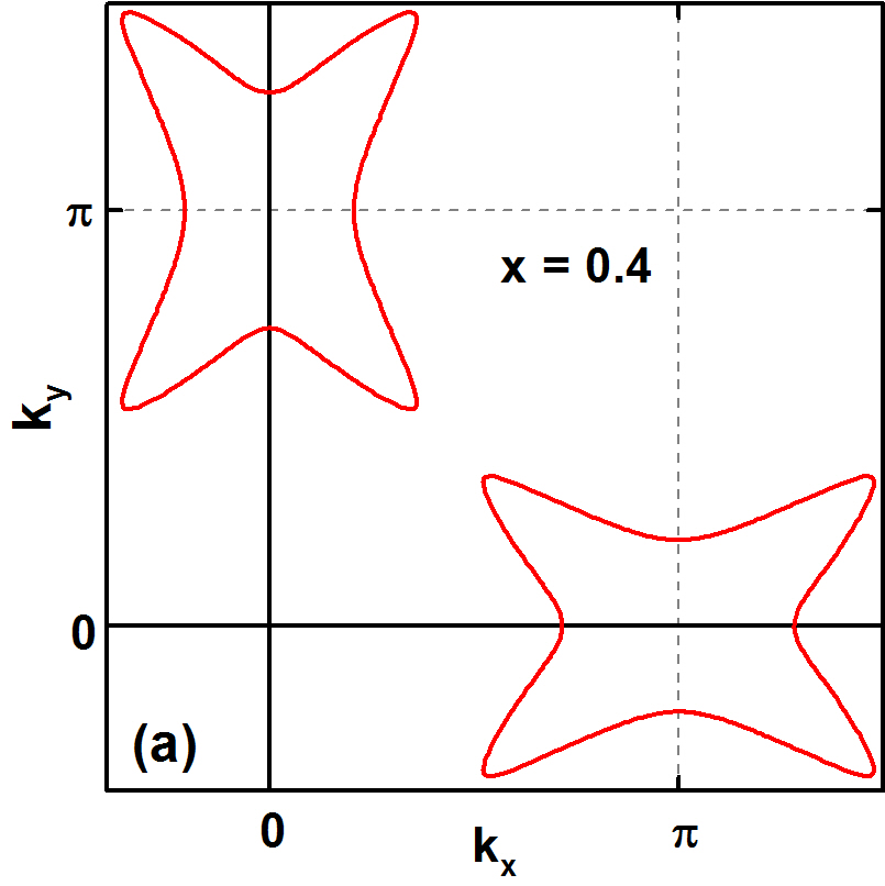
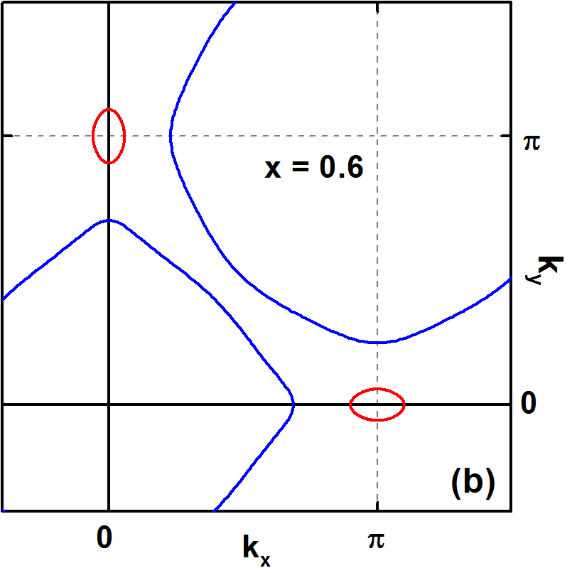
Figure 1: (Color online) Fermi surface at different electron doping values (a) $\text{x}=0.4$ and (b) $\text{x}=0.6$. In panel (a), the electron pockets (red) around $[\pi,0]$ and $[0,\pi]$ will keep increasing in area (as x increases) until they touch (for $\text{x}\approx 0.45$), when a Lifshitz transition occurs and the Fermi surface changes topology to hole pockets (blue) centered around $[0,0]$ and $[\pi,\pi]$ [panel (b)], which will decrease in area as x increases. Finally, as shown in panel (b), small electron pockets (red) emerge around $[\pi,0]$ and $[0,\pi]$ (for $\text{x}\approx 0.5$) and will increase in area as x increases.

2.2 Interacting Hamiltonian

For our model of ${\rm BiS_{2}}$-based superconductors, we will assume that attractive interactions mediate different types of intra- and inter-orbital pairings [1]. The relevant orbitals, as discussed above, are the $p_{X}$ and $p_{Y}$ Wannier orbitals of the Bismuth atoms in a ${\rm BiS}$ plane. The total Hamiltonian of the system can be written as

$$H=H_{0}+H_{I},$$ (3)

where $H_{0}$ is given by eqs. (1) and (2) above and the interacting part of the Hamiltonian can be written as a sum of intra- and inter-orbital components,

$$H_{I} = H_{\rm intra}+H_{\rm inter},$$

where

$$H_{\rm intra} = -\frac{1}{N}\sum_{k,k^{\prime},\alpha}\left(V_{\alpha\alpha\alpha\alpha}~{}p_{\alpha k^{\prime}\uparrow}^{\dagger}p_{\alpha\mathrm{bar}{k}^{\prime}\downarrow}^{\dagger}p_{\alpha\mathrm{bar}{k}\downarrow}p_{\alpha k\uparrow}\right),$$ (4)

$$H_{\rm inter} = -\frac{1}{N}\sum_{k,k^{\prime},\alpha\neq\beta}\Big{(}V_{\alpha\alpha\beta\beta}~{}p_{\alpha k^{\prime}\uparrow}^{\dagger}p_{\alpha\mathrm{bar}{k}^{\prime}\downarrow}^{\dagger}p_{\beta\mathrm{bar}{k}\downarrow}p_{\beta k\uparrow}$$ (5)

$$+ V_{\alpha\beta\beta\alpha}~{}p_{\alpha k^{\prime}\uparrow}^{\dagger}p_{\beta\mathrm{bar}{k}^{\prime}\downarrow}^{\dagger}p_{\beta\mathrm{bar}{k}\downarrow}p_{\alpha k\uparrow}+V_{\alpha\beta\alpha\beta}~{}p_{\alpha k^{\prime}\uparrow}^{\dagger}p_{\beta\mathrm{bar}{k}^{\prime}\downarrow}^{\dagger}p_{\alpha\mathrm{bar}{k}\downarrow}p_{\beta k\uparrow}\Big{)},$$

where $\alpha,\beta=X,Y$, $\mathrm{bar}{k}=-k$, and $N=L^{2}$ is the number of sites in a $L\times L$ square lattice. To be accurate, as we chose the orbital states $p_{X,Y\mathbf{k}\sigma}$ to write the pair operators, we will use the terminology intra- and inter-orbital to refer to the associated pairing, in opposition to intra and interband. The main reason for using the $p_{X,Y\mathbf{k}\sigma}$-orbital states to write the pair operators is that the actual bands [obtained by diagonalizing $H_{0}$] show weak $X-Y$ hybridization, because of the small value of $t_{x}^{XY}=0.107$ in comparison to $t_{x}^{X,Y}=0.880$ (see Table 1). In addition, in systems where many-body terms originating from intra-site interactions may influence superconductivity (see, for example, Ref. [28]), which could be the case for ${\rm BiS_{2}}$ compounds [17], it is advantageous to analyze pairing in the orbital basis.

In the equations above, all the coupling terms $V$ are positive, therefore all pairing interactions considered are attractive. In addition, experimental findings for ${\rm BiS_{2}}$ compounds [18], up to now, support s-wave SC, therefore, we take all the coupling terms as being $\mathbf{k}$-independent. Given that the origin of the pairing interaction in ${\rm BiS_{2}}$ compounds has not been settled yet [17], those are the only general assumptions we will make. In the next two sections we will use symmetry arguments to decrease the number of $V$ terms in eqs. (4) and (5) when applied to ${\rm BiS_{2}}$ compounds.

The inter-orbital terms in eq. (5) may be listed through the associated couplings as ${\rm V_{XXYY}}$ (${\rm V_{YYXX}}$), where an ${\rm YY}$ (${\rm XX}$) pair is scattered into an ${\rm XX}$ (${\rm YY}$) pair; ${\rm V_{XYYX}}$ (${\rm V_{YXXY}}$), where an ${\rm YX}$ (${\rm XY}$) pair is scattered into an ${\rm XY}$ (${\rm YX}$) pair; and ${\rm V_{XYXY}}$ (${\rm V_{YXYX}}$), where an ${\rm XY}$ (${\rm YX}$) pair is scattered into an ${\rm XY}$ (${\rm YX}$) pair. We will see in what follows that, by treating $H_{\rm intra}$ and $H_{\rm inter}$ at the mean-field level, and applying symmetries present in the ${\rm BiS}$ planes, will allow us to reduce these couplings to just two, which we will denote as ${\rm V_{XX}}$ and ${\rm V_{XY}}$.

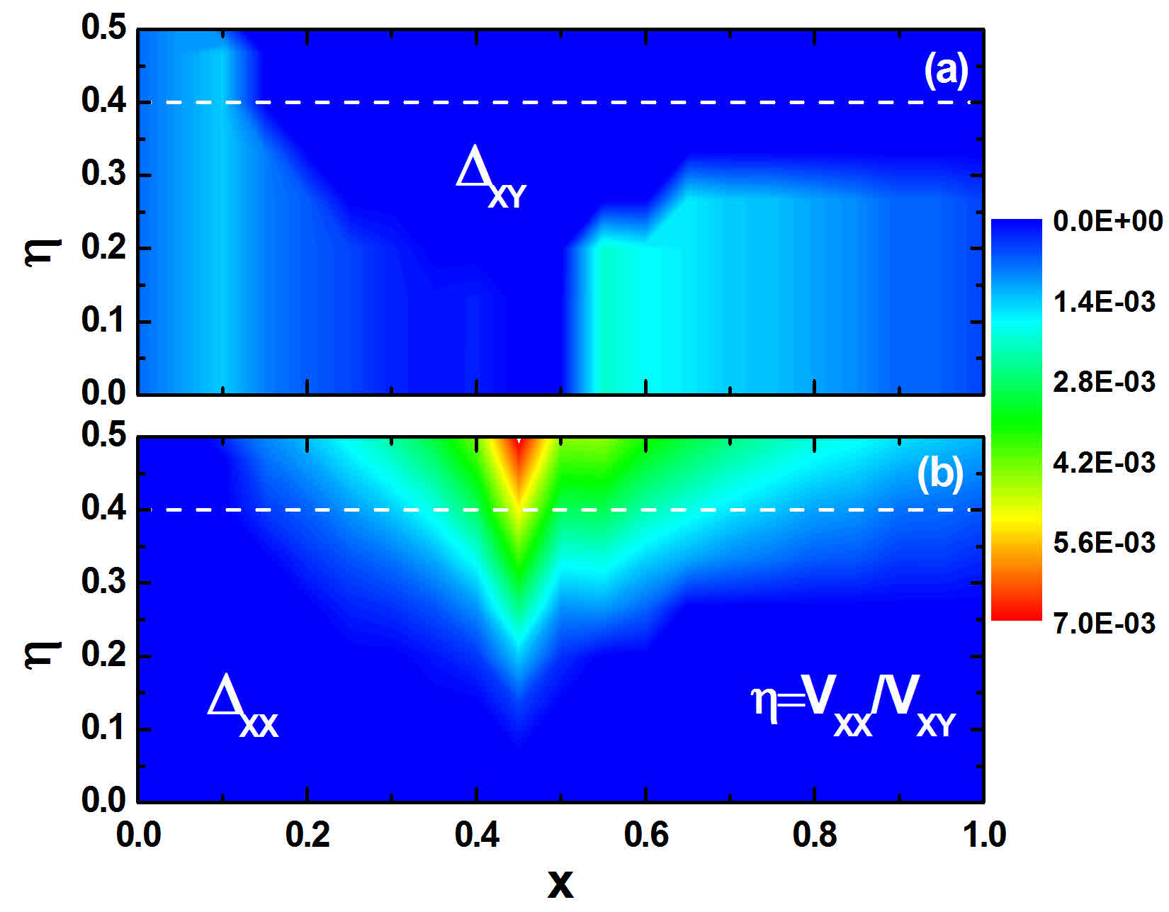
Figure 2: (Color online) ${\rm\Delta_{XY}}$ (a) and ${\rm\Delta_{XX}}$ (b) phase diagram for ${\rm\eta=V_{XX}/V_{XY}}$ vs doping x (gap values in eV). These results were obtained through the self-consistent solution of eqs. 13 and 14 and the parameters used were $V_{XY}=0.19$ eV and $\omega_{D}=10$ meV, which was used as a cutoff for energy integrals in solving the gap equations.

2.3 Mean-field theory and gap equations

The interacting Hamiltonian in eqs. (4) and (5) will be solved at the mean-field level, through the usual approximation $ABCD\approx\langle AB\rangle CD+AB\langle CD\rangle-\langle AB\rangle\langle CD\rangle$:

$$H_{I}\approx H_{MF} = H_{1}+H_{2}+C,$$ (6)

where

$$H_{1} = -\sum_{k}(\Delta_{1}~{}p^{\dagger}_{Xk\uparrow}p^{\dagger}_{X\mathrm{bar}{k}\downarrow}+\Delta_{2}~{}p^{\dagger}_{Yk\uparrow}p^{\dagger}_{Y\mathrm{bar}{k}\downarrow}+h.c.)$$ (7)

and

$$H_{2} = -\sum_{k}(\Delta_{3}~{}p^{\dagger}_{Xk\uparrow}p^{\dagger}_{Y\mathrm{bar}{k}\downarrow}+\Delta_{4}~{}p^{\dagger}_{Yk\uparrow}p^{\dagger}_{X\mathrm{bar}{k}\downarrow}+h.c.),$$ (8)

where $C$ is a constant and the $\Delta_{i}$, which are order parameters of the superconducting phases [29], are given by

$$\Delta_{1} = \frac{1}{N}\sum_{k^{\prime}}V_{XXXX}\langle p_{X\mathrm{bar}{k}^{\prime}\downarrow}p_{Xk^{\prime}\uparrow}\rangle+V_{XXYY}\langle p_{Y\mathrm{bar}{k}^{\prime}\downarrow}p_{Yk^{\prime}\uparrow}\rangle,$$ (9)

$$\Delta_{2} = \frac{1}{N}\sum_{k^{\prime}}V_{YYYY}\langle p_{Y\mathrm{bar}{k}^{\prime}\downarrow}p_{Yk^{\prime}\uparrow}\rangle+V_{YYXX}\langle p_{X\mathrm{bar}{k}^{\prime}\downarrow}p_{Xk^{\prime}\uparrow}\rangle,$$ (10)

$$\Delta_{3} = \frac{1}{N}\sum_{k^{\prime}}V_{XYYX}\langle p_{Y\mathrm{bar}{k}^{\prime}\downarrow}p_{Xk^{\prime}\uparrow}\rangle+V_{XYXY}\langle p_{X\mathrm{bar}{k}^{\prime}\downarrow}p_{Yk^{\prime}\uparrow}\rangle,$$ (11)

$$\Delta_{4} = \frac{1}{N}\sum_{k^{\prime}}V_{YXXY}\langle p_{X\mathrm{bar}{k}^{\prime}\downarrow}p_{Yk^{\prime}\uparrow}\rangle+V_{YXYX}\langle p_{Y\mathrm{bar}{k}^{\prime}\downarrow}p_{Xk^{\prime}\uparrow}\rangle.$$ (12)

2.4 Applying symmetries

We start our analysis from the fact that ${\rm V_{XXYY}=V_{YYXX}}$ and ${\rm V_{XYYX}=V_{YXXY}}$. Now, to simplify eqs. (9) to (12), we will apply some symmetry properties related to the Bismuth $p_{X}$ and $p_{Y}$ orbitals, which lead to relations between the remaining couplings ${\rm V}$ and between the expectation values in those equations. Given that both orbitals have the same energy and are related by a $C_{4}$ rotation [22], we expect that ${\rm V_{XXXX}=V_{YYYY}}$ and $\langle p_{X\mathrm{bar}{k}^{\prime}\downarrow}p_{Xk^{\prime}\uparrow}\rangle=\langle p_{Y\mathrm{bar}{k}^{\prime}\downarrow}p_{Yk^{\prime}\uparrow}\rangle$. Therefore, $\Delta_{1}=\Delta_{2}$ (which we now denote as ${\rm\Delta_{XX}}$), and, if we define ${\rm V_{XX}\equiv V_{XXXX}+V_{XXYY}}$, we obtain

$$\Delta_{XX} = -\frac{V_{XX}}{N}\sum_{k^{\prime}}\langle p_{X\mathrm{bar}{k}^{\prime}\downarrow}p_{Xk^{\prime}\uparrow}\rangle.$$ (13)

Note that the above equation replaces eqs. (9) and (10). The same symmetry arguments lead to ${\rm V_{XYXY}=V_{YXYX}}$ and $\langle p_{Y\mathrm{bar}{k}^{\prime}\downarrow}p_{Xk^{\prime}\uparrow}\rangle=\langle p_{X\mathrm{bar}{k}^{\prime}\downarrow}p_{Yk^{\prime}\uparrow}\rangle$, which result in $\Delta_{3}=\Delta_{4}$ (which we now denote as ${\rm\Delta_{XY}}$), and, if we define ${\rm V_{XY}\equiv V_{XYYX}+V_{XYXY}}$, we obtain

$$\Delta_{XY} = -\frac{V_{XY}}{N}\sum_{k^{\prime}}\langle p_{Y\mathrm{bar}{k}^{\prime}\downarrow}p_{Xk^{\prime}\uparrow}\rangle.$$ (14)

Note that the above equation replaces eqs. (11) and (12).

The simplified gap equations (13) and (14) determine the system of self-consistent equations to be solved, where the effective interactions ${\rm V_{XX}}$ and ${\rm V_{XY}}$ are parameters that control pairing of same-orbital electrons (${\rm XX}$ or ${\rm YY}$), or dissimilar electrons (${\rm XY}$ or ${\rm YX}$), respectively. We stress that the order parameter ${\rm\Delta_{XX}}$ involves both intra-orbital (${\rm XX\leftrightarrow XX}$ and ${\rm YY\leftrightarrow YY}$) as well as inter-orbital (${\rm XX\leftrightarrow YY}$) processes, while the order parameter ${\rm\Delta_{XY}}$ involves only inter-orbital processes (${\rm XY\leftrightarrow YX}$, ${\rm XY\leftrightarrow XY}$, and ${\rm YX\leftrightarrow YX}$).

Figure 2 shows the results obtained by self-consistently solving eqs. (13) and (14) for both ${\rm\Delta_{XY}}$, in panel (a), and ${\rm\Delta_{XX}}$, in panel (b). The phase diagram presents a color map plot of both gap functions in the $\eta$ vs x plane, where ${\rm\eta=V_{XX}/V_{XY}}$ measures the ratio between the couplings (${\rm V_{XY}=0.19~{}eV}$ was kept constant while ${\rm V_{XX}}$ varied). The color scale is the same for both panels and it is given in eV units. Details of the self-consistent numerical solution of the gap equations can be found in Ref. [[24]].

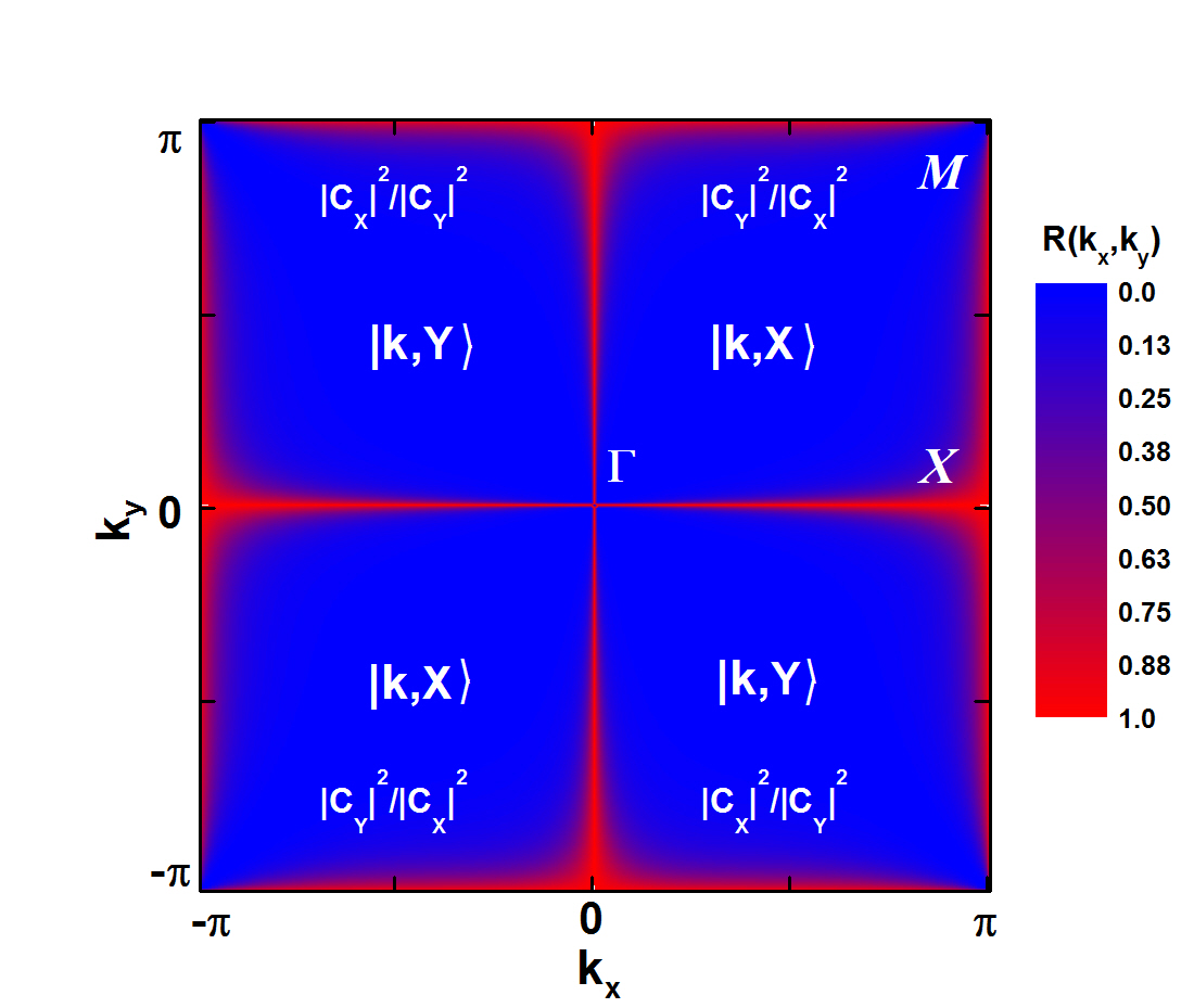
Figure 3: (Color online) Variation along the BZ of the orbital-mixing ratio $R(k_{x},k_{y})=|C_{X,Y}|^{2}/|C_{Y,X}|^{2}$ for the lower energy band, showing that a well defined orbital character (either $|k,X\rangle$ or $|k,Y\rangle$, for $R(k_{x},k_{y})\approx 0$) alternates from one quadrant to the next, with the orbital mixed character ($R(k_{x},k_{y})\approx 1$) concentrated along the crystallographic axes. Note that, as indicated in the figure, the choice of the $X$ and $Y$ subindexes in the definition of $R(k_{x},k_{y})$ for each quadrant is such that $0\leq R(k_{x},k_{y})\leq 1$ for the whole BZ. The results for the higher energy band are identical to the ones shown here, but with $X$ and $Y$ swapped.

3 Results and Discussion

3.1 Orbital-mixing and multiband superconductivity

The superconducting state emerges from an instability of the Fermi sea (metallic normal state) to an attractive effective interaction. This interaction forms Cooper pairs that scatter against each other, always conserving total momentum and individual spin, while staying in a shell around the Fermi surface. It is then expected that many properties of the superconducting state, like the gap function and, in a multiband system, the possibility of the existence of different types of Cooper pairs, will be directly associated to the properties of the Fermi surface in the normal state. Thus, in a system like ${\rm BiS_{2}}$, whose Fermi surface varies widely with electron doping, even showing a Lifshitz transition, as illustrated in Fig. 1, one would expect that the superconducting gap function should also show a marked variation with electron doping. Indeed, the gap function results in Fig. 2 clearly confirm this expectation by showing very marked variations when the system goes through the Lifshitz transition (for $\text{x}\approx 0.45$). However, as described in this section, our results, when analyzed more carefully, also show that there is a more subtle aspect relating multiband SC with the nature of the band states at the Fermi surface. This aspect, once properly quantified, can be directly linked to the very particular electronic structure of ${\rm BiS_{2}}$ compounds. As will be illustrated below, the orbital-mixing character of a band state changes from point to point in the BZ of ${\rm BiS_{2}}$, varying continuously from pure-${\rm X}$ to pure-${\rm Y}$ (and back, passing by completely-${\rm XY}$-mixed) in accordance to symmetry requirements. As a consequence, the degree of mixing of the ${\rm X}$- and ${\rm Y}$-orbital at the Fermi surface, for a particular electron doping, may change between different regions of the Fermi surface. This is not surprising in itself. What is interesting in the case of ${\rm BiS_{2}}$ is that the systematic variation of the orbital-mixing along the ${\rm BiS_{2}}$ Fermi surface can be semi-quantitatively connected to the ${\rm\Delta_{XY}}$ and ${\rm\Delta_{XX}}$ results in Fig. 2.

Therefore, we will use the idea of orbital-mixing, as defined below, as well as the way the Fermi surface changes with doping, to explain the main structures seen in the superconducting gap functions shown in Fig. 2, as, for example, the position of the maxima and minima of ${\rm\Delta_{XY}}$ and ${\rm\Delta_{XX}}$ as a function of electron doping x. Note that we assume a rigid band situation (i.e., doping does not change the band structure); ARPES results [18] have shown that this is a good approximation for ${\rm BiS_{2}}$ compounds.

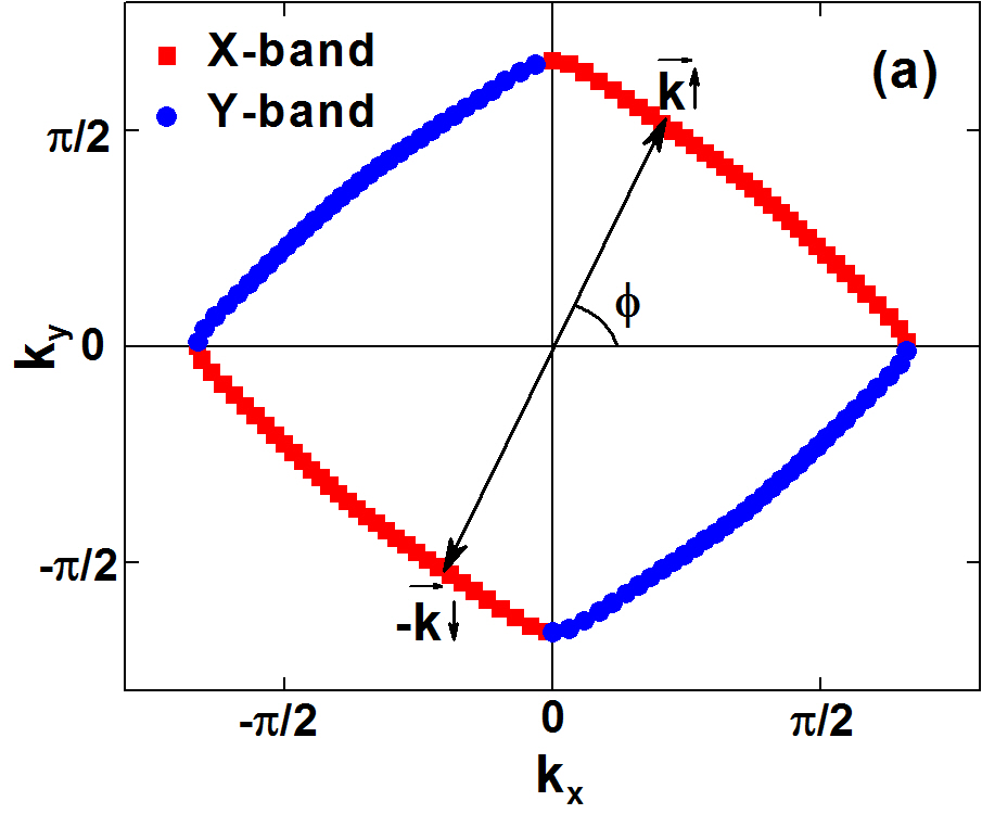
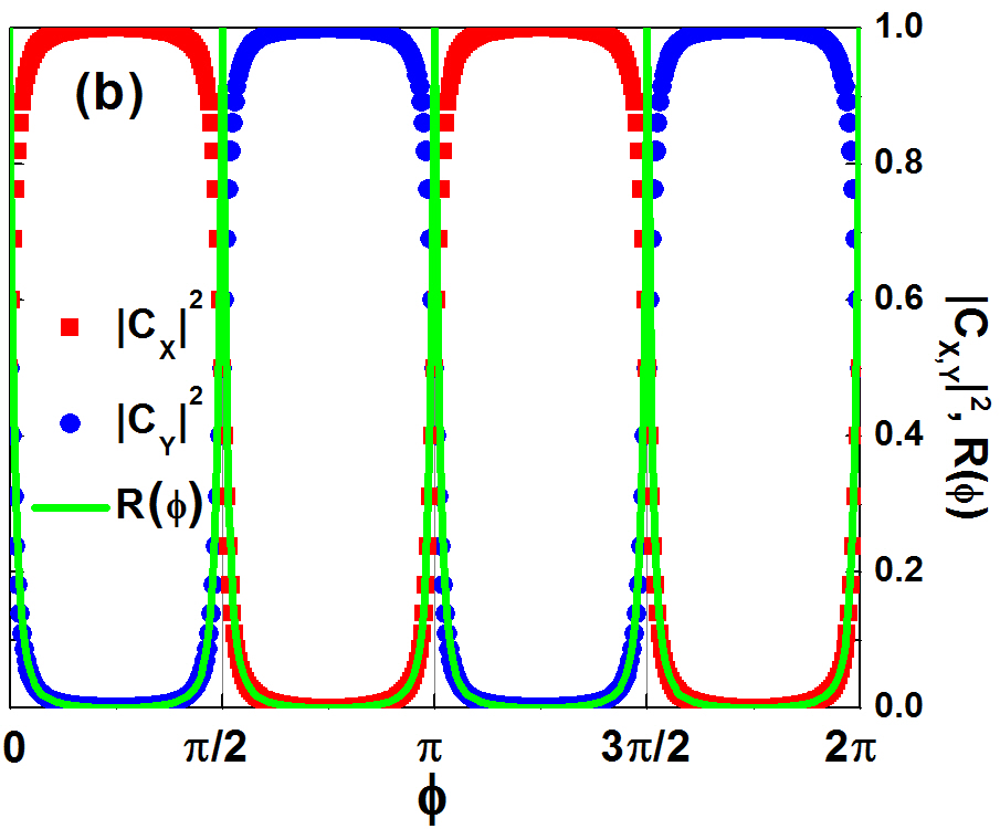
Figure 4: (Color online) (a) Example of a hole pocket centered around $[0,0]$ with almost zero-mixing ($\text{x}=0.75$): the well defined ${\rm X}$-orbital [(red) squares] or ${\rm Y}$-orbital [(blue) circles] character of the Fermi surface states changes from one quadrant to the next. This well defined character is determined by $|C_{X,Y}|^{2}\approx 1.0$, where a generic band state at the Fermi surface is written as $|\vec{k}\rangle=C_{X}|p_{k,X}\rangle+C_{Y}|p_{k,Y}\rangle$. (b) $|C_{X}|^{2}$ [(red) squares] and $|C_{Y}|^{2}$ [(blue) circles] values around the Fermi surface ($0\leq\phi\leq 2\pi$) for the hole pocket in panel (a). The solid (green) curve shows the corresponding results for $R(\phi)$, the orbital-mixing ratio, which vanishes for most of the Fermi surface, aside from very small regions around multiples of $\pi/2$ where symmetry imposes an ${\rm X\leftrightarrow Y}$ swap of the orbital character of the band states. In panel (a), a generic Cooper pair will be of ${\rm XX}$- (as depicted) or ${\rm YY}$-type, no ${\rm XY}$-type being possible.

Consider a band state, at a generic $\mathbf{k}=[k_{x},k_{y}]$ in the first BZ, written as $|\mathbf{k}\rangle=C_{X}(k_{x},k_{y})|p_{X,k}\rangle+C_{Y}(k_{x},k_{y})|p_{Y,k}\rangle$, where $|p_{\alpha,k}\rangle=p^{\dagger}_{\alpha\mathbf{k}}|vac\rangle$, for $\alpha=X$, $Y$ (where the spin index was omitted for the sake of brevity). To quantify the degree of orbital-mixing, we define $R(k_{x},k_{y})=|C_{\alpha}(k_{x},k_{y})|^{2}/|C_{\beta}(k_{x},k_{y})|^{2}$, where $\alpha$ and $\beta$ take values $X$ or $Y$ such that $0.0\leq R(k_{x},k_{y})\leq 1.0$ for all $[k_{x},k_{y}]$. Thus, we refer to $R(k_{x},k_{y})$ as the orbital-mixing ratio between the ${\rm X}$-orbital and ${\rm Y}$-orbital for each point of the BZ, where $R(k_{x},k_{y})=1.0$ indicates maximum orbital mixing, where the band state does not have a well defined ${\rm X}$- or ${\rm Y}$-orbital character, being an equal mix of both; and $R(k_{x},k_{y})=0.0$ indicates no orbital mixing at all, i.e., the band state has a well defined (either ${\rm X}$- or ${\rm Y}$-) orbital character. We will refer to the former as a orbital-mixed band state and to the latter as a zero-mixing band state.

Figure 3 shows a color-map plot of $R(k_{x},k_{y})$ for the lower energy band in the first BZ. As indicated by the labels, a well defined orbital character can be associated to the band states (denoted as either $|k,X\rangle$, when $|C_{X}(k_{x},k_{y})|\approx 1$, or $|k,Y\rangle$, when $|C_{Y}(k_{x},k_{y})|\approx 1$) in a wide range around the $\Gamma M$ symmetry lines (where $R(k_{x},k_{y})\approx 0$) in each quadrant (alternating from $|k,X\rangle$ to $|k,Y\rangle$ from one quadrant to the next), while the band states in a narrow region around the $\Gamma X$ and $XM$ symmetry lines are orbital-mixed ($R(k_{x},k_{y})\approx 1$). Results for the higher energy band are identical, but for the swapping of $X$ and $Y$. Based on these results, parts of the Fermi surface that are formed by large hole pockets around the $\Gamma$ and M points in the BZ [see Fig. 1(b)] contain mostly band states with zero-mixing, while parts of the Fermi surface formed by smaller electron pockets around the X points in the BZ will contain band states with a larger degree of orbital mixing. In what follows, we will analyze the orbital-mixing ratio $R(k_{x},k_{y})$ over Fermi surface pockets, i.e., we will be interested on the variation of $R(\phi)$ as we move around the pocket’s edge, where we have parametrized $\vec{k}_{F}$ as $[k_{F},\phi]$, where $\phi$ is the polar angle measured around the pocket’s center.

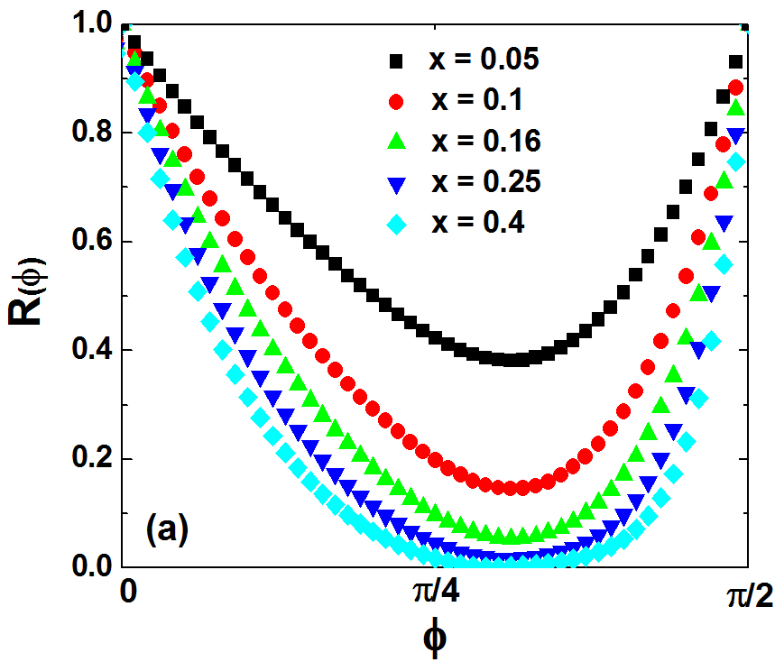
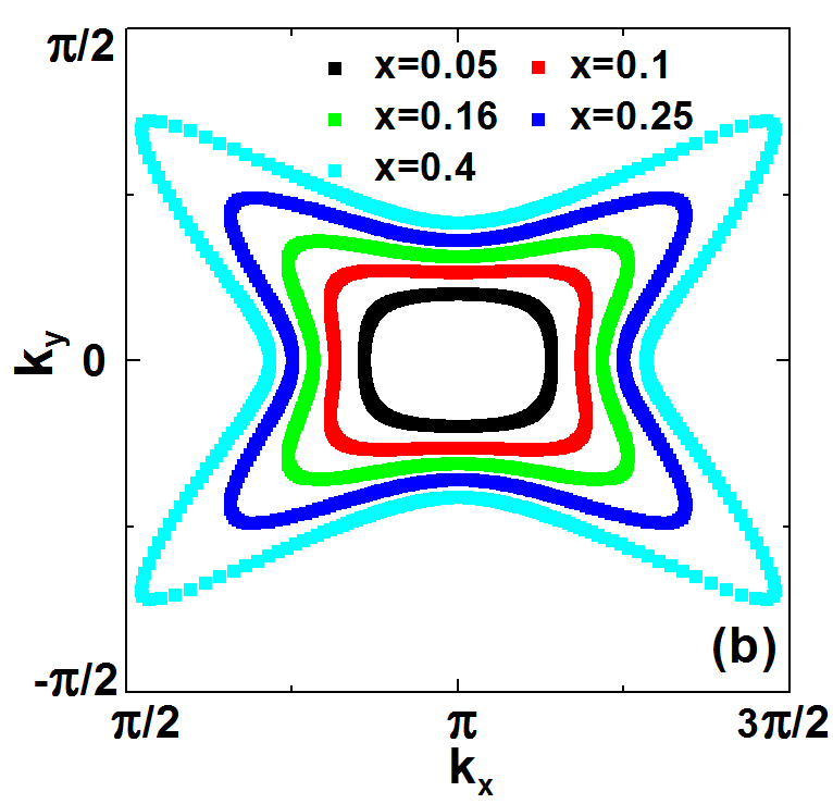
Figure 5: (Color online) (a) $R(\phi)$ (see text for definition) in the first quadrant of the $[\pi,0]$ electron pocket for $\text{x}=0.05$ [(black) squares], $\text{x}=0.1$ [(red) circles], $\text{x}=0.16$ [(green) up triangles], $\text{x}=0.25$ [(blue) down triangles], and $\text{x}=0.4$ [(cyan) diamonds]. (b) $[\pi,0]$ electron pockets for the same values of x as in panel (a).

To clarify the connection between orbital-mixing and Cooper pair formation in a multiband system and therefore develop an intuitive picture of the relation between the ${\rm\Delta_{XY,XX}}$ superconducting order parameters and orbital-mixing, we show in Fig. 4(a) the zero-mixing case for a hole pocket around $[0,0]$ obtained for $\text{x}=0.75$, with the corresponding values for $|C_{X}|^{2}$ [(red) squares], $|C_{Y}|^{2}$ [(blue) circles], and $R(\phi)$ [(green) solid curve] shown in Fig. 4(b), where we see that $R(\phi)\approx 0$ for the whole pocket with the exception of small regions around $\phi$ values that are multiples of $\pi/2$, where symmetry imposes an $X\leftrightarrow Y$ swap in the $|C_{X,Y}|^{2}$ coefficients [22]. Therefore, in a zero-mixing pocket, if states at the Fermi surface have very well defined orbital character in one specific quadrant [${\rm X}$-orbital, for example, in the first quadrant, as shown in Fig. 4(a)], they will have the opposite character in the next quadrant [${\rm Y}$-orbital in the second quadrant in Fig. 4(a)], and so on. In that case, Cooper pairs will be formed by ${\rm X}$-orbital electrons only [${\rm XX}$ pairs, like the one depicted in panel (a)] or ${\rm Y}$-orbital electrons only (${\rm YY}$ pairs). Exchange of phonons that scatter electrons between opposing quadrants will lead to ${\rm XX\leftrightarrow XX}$ and ${\rm YY\leftrightarrow YY}$ pair scattering, while phonons that scatter electrons between adjacent quadrants will lead to ${\rm XX\leftrightarrow YY}$ pair scattering. Therefore, zero-mixing pockets are associated to the SC order parameter ${\rm\Delta_{XX}}$. On the other hand, for electron pockets around the X points in the BZ, where orbital-mixing dominates i.e., $|C_{X}|^{2}\approx|C_{Y}|^{2}\approx 1/2$, formation of $p^{\dagger}_{X,k,\uparrow}p^{\dagger}_{Y,-k,\downarrow}$ pairs becomes possible, therefore, the order parameter ${\rm\Delta_{XY}}$ is connected to orbital-mixed pockets.

It is important to realize at this point that the results shown in Fig. 3, for $R(k_{x},k_{y})$, are obviously independent of the electron doping x. However, since we are interested in what happens at the Fermi surface, as the pockets continuously expand or contract as x varies (see Fig. 1), causing their edges to sweep through the BZ, $R(\phi)$ at the edge of each pocket will change substantially with electron doping for electron pockets centered around X points in the BZ (see Figs. 5 and 6), while it will change very little for hole pockets centered around the $\Gamma$ and M points in the BZ [see Fig. 7(a)]. Therefore, in what follows, when we refer to changes in $R(\phi)$ with electron doping, that is what is meant.

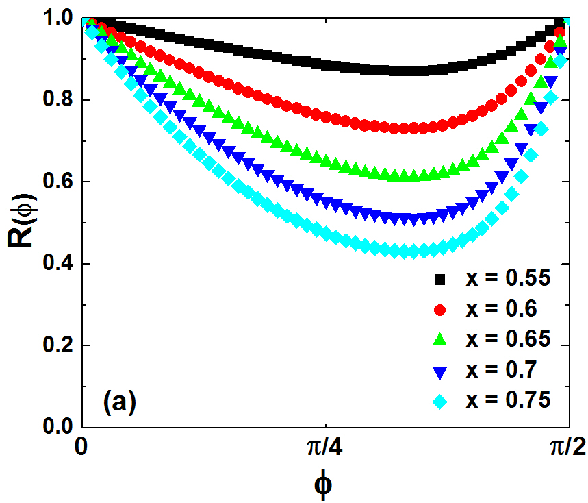
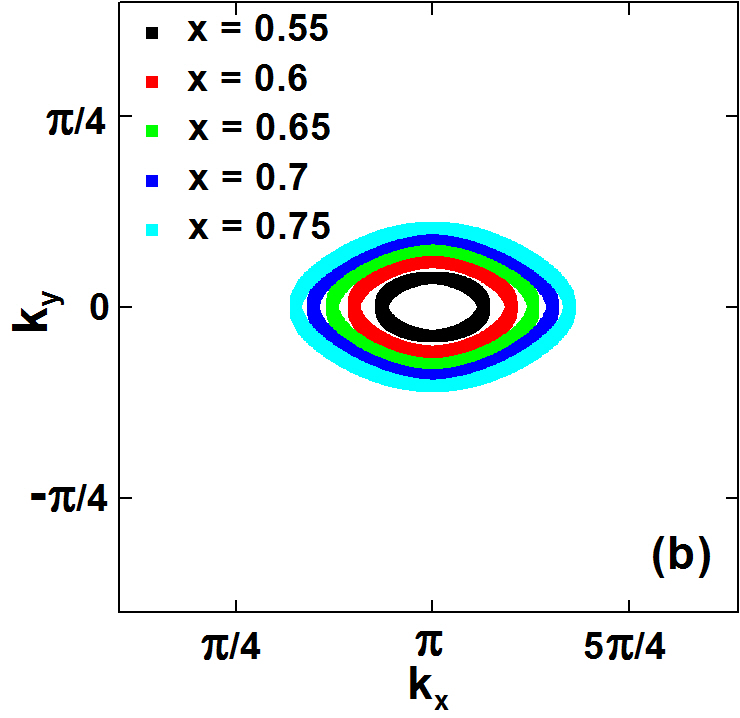
Figure 6: (Color online) Same as in Fig. 5, but now for $\text{x}=0.55$ [(black) squares], $\text{x}=0.6$ [(red) circles], $\text{x}=0.16$ [(green) up triangles], $\text{x}=0.7$ [(blue) down triangles], and $\text{x}=0.75$ [(cyan) diamonds].

3.2 Orbital-mixing and multiband SC below the Lifshitz transition

Now, using $R(\phi)$ as a measure of orbital-mixing, we will qualitatively connect the structures seen in the gap function results in Fig. 2 to the way $R(\phi)$ varies with doping. Let us start at x values below the Lifshitz transition, which occurs for $\text{x}\approx 0.45$, where the Fermi surface changes from electron pockets centered around $[\pi,0]$ and $[0,\pi]$ to hole pockets centered around $[0,0]$ and $[\pi,\pi]$ (see Fig. 1). In Fig. 5(a) we show $R(\phi)$ results for the first quadrant of the electron pocket around $[\pi,0]$ for 5 different values of doping $0.05\leq\text{x}\leq 0.4$. In Fig. 5(b) it is shown how the size of the $[\pi,0]$ electron pocket increases with electron doping for the same x values as in panel (a). Given the $C_{4}$ symmetry of ${\rm BiS_{2}}$, the pattern shown in Fig. 5(a) repeats itself for all quadrants, with the appropriate $X\leftrightarrow Y$ swap in the definition of $R(\phi)$ [30]. The results in Fig. 5(a) show a decrease in mixing as the doping increases. Referring to Fig. 3, it is easy to see that this is due to the increase in size of the electron pockets centered around the X points in the BZ [see Fig.5(b)]: as these pockets increase, larger parts of the Fermi surface will be in $R(\phi)\approx 0$ regions of the BZ. Keeping in mind, as discussed above, that ${\rm\Delta_{XY}}$ is associated to orbital-mixing ($R(\phi)\approx 1$) and ${\rm\Delta_{XX}}$ with the absence of it ($R(\phi)\approx 0$), one should then expect, as x varies, a maximum (at low doping) in ${\rm\Delta_{XY}}$ and a steady increase in ${\rm\Delta_{XX}}$. Indeed, if one takes a fixed $\eta=0.4$, for example, in Fig. 2 (see dashed line in both panels), and contrasts how ${\rm\Delta_{XY}}$ and ${\rm\Delta_{XX}}$ vary as x increases from zero, that is exactly what happens.

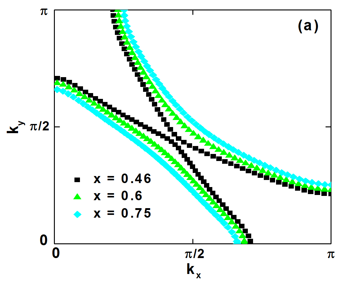
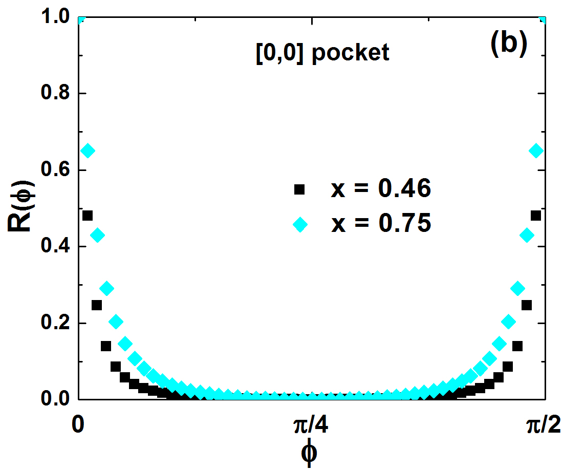
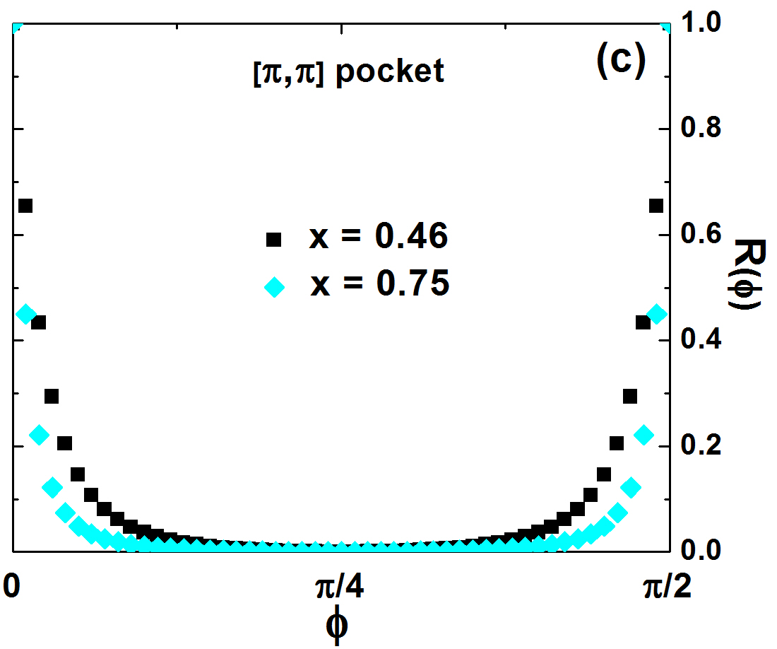
Figure 7: (Color online) (a) Doping variation of the $[0,0]$ and $[\pi,\pi]$ hole pockets for $\text{x}=0.46$ [(black) squares], $\text{x}=0.6$ [(green) up triangles], and $\text{x}=0.75$ [(cyan) diamonds] (b) $R(\phi)$ in the first quadrant of the $[0,0]$ hole pocket [in panel (a)] for $\text{x}=0.46$ [(black) squares] and $\text{x}=0.75$ [(cyan) diamonds]. (c) Same as in panel (b), but now for the $[\pi,\pi]$ hole pocket in panel (a).

3.3 Orbital-mixing and multiband SC above the Lifshitz transition

Now, using the same ideas as in the previous section, we will explain the main structures of ${\rm\Delta_{XY}}$ and ${\rm\Delta_{XX}}$ at, and above, the Lifshitz transition. As mentioned above, as one approaches the Lifshitz transition (at $\text{x}\approx 0.45$) from below (and the $[\pi,0]$ and $[0,\pi]$ electron pockets are about to touch and become hole pockets around $[0,0]$ and $[\pi,\pi]$) $R(\phi)\approx 0$ over the full extension of the Fermi surface, causing ${\rm\Delta_{XY}}$ to vanish. In reality, as the $R(\phi)$ results in Fig. 5 show, ${\rm\Delta_{XY}}$ should have essentially vanished for $\text{x}\approx 0.2$, which agrees with the results in Fig. 2. Figure 6 explains the behavior of ${\rm\Delta_{XY}}$ for $\text{x}>0.55$, where, as shown in Fig. 6(b), an electron pocket around $[\pi,0]$ forms again and increases with x. Fig. 6(a) shows that this pocket initially presents strong orbital-mixing ($R(\phi)\approx 1.0$ for the whole pocket), which slowly decreases as the pocket increases, leading to the broad maximum in ${\rm\Delta_{XY}}$ around $\text{x}\approx 0.6$, as seen in Fig. 2(a).

As to ${\rm\Delta_{XX}}$, at the Lifshitz transition it should reach a maximum, since, above it, the hole pockets $[0,0]$ and $[\pi,\pi]$ will start decreasing (as x keeps increasing). This is shown in Fig. 7(a) for $\text{x}=0.46$ [(black) squares], $\text{x}=0.6$ [(green) up triangle], and $\text{x}=0.75$ [(cyan) diamonds]. The behavior of $R(\phi)$ for $\text{x}=0.46$ and $\text{x}=0.75$ is shown in Fig. 7(b) for the $[0,0]$ hole pocket and 7(c) for $[\pi,\pi]$. As expected, based on the results shown in Fig. 3, the orbital-mixing ratio $R(\phi)$ is very small for both pockets at $\text{x}=0.46$ [(black] squares) and it barely changes between $\text{x}=0.55$ (not shown) and $\text{x}=0.75$ [(red) circles], indicating that these pockets only contribute to ${\rm\Delta_{XX}}$, as discussed above. Therefore, a somewhat broad maximum in ${\rm\Delta_{XX}}$, as shown in Fig. 2(b), occurs around the Lifshitz transition at $\text{x}\approx 0.46$ and it is associated to the larger Fermi surface at this doping. Incidentally, the largest gap value in Fig. 2 is that for ${\rm\Delta_{XX}}$ right after the Lifshitz transition, when the $[0,0]$ and $[\pi,\pi]$ hole pockets have maximum size and basically no mixture.

3.4 Critical Temperature Results

Figure 8 shows results for the superconducting critical temperature $T_{c}$ vs x obtained from a plot (not shown) very similar to the one in Fig. 2. The parameters used for calculating $T_{c}$ were $V_{XY}=0.16$ eV, $\omega_{D}=5$ meV, and ${\rm\eta=V_{XX}/V_{XY}}=0.7$. We used slightly smaller parameter values from the ones used in Fig. 2 so that the maximum $T_{c}\approx 10$ K is similar to that measured for ${\rm BiS_{2}}$ compounds [31]. A comparison with a compilation of $T_{c}$ values for ${\rm LnO_{1-x}F_{x}BiS_{2}}$ (where Ln = La, Ce, Pr, and Nd) [see Fig. 2 in Ref. [31]], shows an overall similarity with the results in Fig. 8: $T_{c}\approx 2$ K for $\text{x}=0.1$, $T_{c}\approx 6$ K for $\text{x}\approx 0.6$, and (for Ln = Nd) a dip in $T_{c}$ for larger values of x. Our results, therefore, are in good qualitative agreement with experimental results for ${\rm BiS_{2}}$ compounds. The $T_{c}$ values were obtained by solving, for a fixed value of x, eqs. 13 and 14 self-consistently for temperatures $T\geq 0$; then, a critical temperature associated to each diferent gap, ${\rm\Delta_{XY}}$ [(blue) circles] or ${\rm\Delta_{XX}}$ [(red) squares], is determined once the corresponding gap value falls below $10^{-6}$.

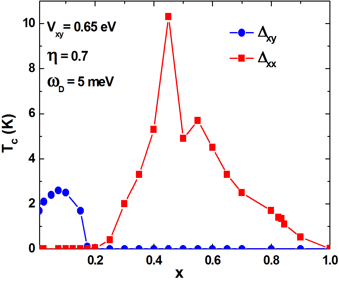
Figure 8: (Color online) Results for the superconducting critical temperature $T_{c}$ vs x obtained from a plot very similar to that on Fig. 2. The parameter values used here were $V_{XY}=0.16$ eV, $\omega_{D}=5$ meV, and ${\rm\eta=V_{XX}/V_{XY}}=0.7$. A smaller value of $\omega_{D}$ than in Fig. 2 was used to insure that the maximum $T_{c}$ value is close to that of $\rm BiS_{2}$ compounds [31].

4 Summary and Conclusions

In summary, we have presented results for a mean-field treatment of a model for multiband SC of ${\rm BiS_{2}}$-based layered compounds, using as starting point a minimal two-orbital tight-binding model, known to reproduce the main properties of the Fermi surface of ${\rm LaO_{(1-x)}F_{x}BiS_{2}}$, including its variation with electron doping. In this minimal model, the bands crossing the Fermi surface originate from the ${\rm 6p_{X}}$ and ${\rm 6p_{Y}}$ Bismuth orbitals (labeled ${\rm X}$- and ${\rm Y}$-orbital). The attractive pair-scattering part of the Hamiltonian allows for the formation of all three types of Cooper pairs (${\rm XX}$, ${\rm YY}$, and ${\rm XY}$), resulting in (after symmetry considerations) two gap equations involving superconducting order parameters ${\rm\Delta_{XX}}$ (associated to pair scatterings of the type ${\rm XX\leftrightarrow XX}$, ${\rm YY\leftrightarrow YY}$, and ${\rm XX\leftrightarrow YY}$) and ${\rm\Delta_{XY}}$ (${\rm XY\leftrightarrow XY}$). The self-consistent numerical solution of the gap equations was presented as a function of ${\rm\eta=V_{XX}/V_{XY}}$, the ratio between the pairing couplings, and the electron doping x. We then defined the quantity $R(k_{x},k_{y})$, which measures the degree of ${\rm X}$- and ${\rm Y}$-orbital mixing of a band state, and used its value $0\leq R(\phi)\leq 1$ to classify the Fermi surface pockets (parametrized through the polar angle $\phi$) as zero-mixing ($R(\phi)\approx 0$) or orbital-mixed ($R(\phi)\approx 1$). The definition of $R(\phi)$ allowed us to identify two distinct situations regarding SC: (i) zero-mixing pockets allow the formation of ${\rm XX}$ and ${\rm YY}$ pairs only, promoting ${\rm XX\leftrightarrow XX}$, ${\rm YY\leftrightarrow YY}$, and ${\rm XX\leftrightarrow YY}$ pair scattering, and therefore strengthens the ${\rm\Delta_{XX}}$ order parameter (or, as we call it, ${\rm XX}$-type SC), while (ii) orbital-mixed pockets result in ${\rm XY}$ pairs, promoting ${\rm XY\leftrightarrow XY}$ pair scattering and strengthening the ${\rm\Delta_{XY}}$ order parameter (${\rm XY}$-type SC). Calculating $R(k_{x},k_{y})$ in the first BZ we could assert that hole pockets around $[0,0]$ and $[\pi,\pi]$ are mostly zero-mixing and small electron pockets around $[0,\pi]$ and $[\pi,0]$ are mostly orbital-mixed, becoming gradually zero-mixing as they increase in size. Based on that, and knowing how the Fermi surface pockets evolve with doping, we could semi-quantitatively predict the main structures observed in the ${\rm\Delta_{XY}}$ and ${\rm\Delta_{XX}}$ phase diagrams. In regions of the parameter space where both order parameters are present, we have, in general, that ${\rm\Delta_{XX}}\gg{\rm\Delta_{XY}}$, unless $\eta\ll 1$. This can be explained by the relative size of the areas in the first BZ where $R(k_{x},k_{y})\approx 0$ or $R(k_{x},k_{y})\approx 1$, with the former taking a much larger share of the first BZ. This implies that, unless the Fermi surface is restricted to small electron pockets around the X points, which only occurs at very low doping, ${\rm XX}$-type SC will always dominate (unless $\eta\ll 1$). Finally, we also showed results for the superconducting critical temperature $T_{c}$, as a function of doping x, which are in qualitative agreement with those measured for ${\rm BiS_{2}}$ compounds.

In conclusion, in this work we present results for a particularly simple model of multiband SC, describing ${\rm BiS_{2}}$ compounds, where the two bands crossing the Fermi surface originate from symmetry-related orbitals, and for which all types of Cooper pairs are allowed. The results for the two superconducting order parameters obtained can be semi-quantitatively linked to the way $R(\phi)$, the orbital-mixing ratio, changes as the Fermi surface evolves with electron doping. Given the current importance of multiband SC and the availability of computational techniques to produce effective models, at the tight-binding level, that describe the normal phase Fermi surface with relative accuracy, we envisage the use of the ideas here presented to spot favorable regions in the phase diagram (controlled mostly by carrier doping) to analyze specific aspects of multiband SC. For example, as clearly shown in this work, the use of the orbital-mixing ratio $R(\phi)$ allows us to correctly infer that ${\rm\Delta_{XY}}$ dominates at low electron doping, while ${\rm\Delta_{XX}}$ dominates close to the Lifshitz transition. This type of information could guide experimentalists into where to investigate for phenomena associated to each different order parameter. We hope that this approach would be appealing to experimental research groups interested in pinpointing favorable scenarios to observe such elusive phenomena as Leggett modes [3] or the Fulde-Ferrell-Larkin-Ovchinnikov state, [19, 20] which are associated to multiband SC. Finally, we also speculate that one could use these ideas to propose simple effective multiband models with the appropriate Fermi surfaces and orbital mixing, which will lead, at the appropriate band filling, to the dominance of one, or the other, of the superconducting order parameters. This could lead to proposals for real materials that could be described by these effective simple models, completing a reverse engineering strategy.

References

- [1] Suhl H, Matthias B T and Walker L R 1959 Phys. Rev. Lett. 3(12) 552
- [2] R. Micnas, S. Robaszkiewicz, and A. Bussmann-Holder, “Two-Component Scenarios for Non-Conventional (Exotic) Superconductors” in Superconductivity in Complex Systems, Structure and Bonding, vol. 114, K. A. Müller and A. Bussmann-Holder (eds.) (Springer-Verlag, Berlin Heilderberg, 2005).
- [3] Lin S Z 2014 J. Phys. Condens. Matter 26 493202
- [4] Buzea C and Yamashita T 2001 Supercond. Sci. Technol. 14 R115
- [5] Xi X X 2008 Rep. Prog. Phys. 71 116501
- [6] Seyfarth G, Brison J P, Méasson M A, Flouquet J, Izawa K, Matsuda Y, Sugawara H and Sato H 2005 Phys. Rev. Lett. 95(10) 107004
- [7] Jourdan M, Zakharov A, Foerster M and Adrian H 2004 Phys. Rev. Lett. 93(9) 097001
- [8] Floris A, Sanna A, Laders M, Profeta G, Lathiotakis N N, Marques M A L, Franchini C, Gross E K U, Continenza A and Massidda S 2007 Phys. C 456 45
- [9] Platt C, Hanke W and Thomale R 2013 Adv. Phys. 62 453
- [10] P K Biswas, and A Amato, and C Baines, and R Khasanov, and H Luetkens, and H Lei, and C Petrovic, and E Morenzoni 2013 Phys. Rev. B 88 224515
- [11] Tanaka Y 2015 Supercond. Sci. Technol. 28 034002
- [12] Kondo J 1963 Progr. Theor. Phys. 29 1
- [13] Bardeen J, Cooper L N and Schrieffer J R 1957 Phys. Rev. 108(5) 1175
- [14] Ding H, Richard P, Nakayama K, Sugawara K, Arakane T, Sekiba Y, Takayama A, Souma S, Sato T, Takahashi T, Wang Z, Dai X, Fang Z, Chen G F, Luo J L and Wang N L 2008 EPL 83 47001
- [15] Iavarone M, Karapetrov G, Koshelev A E, Kwok W K, Crabtree G W, Hinks D G, Kang W N, Choi E M, Kim H J, Kim H J and Lee S I 2002 Phys. Rev. Lett. 89(18) 187002
- [16] G. Gladstone, M. A. Jensen, and J. R. Schrieffer “Superconductivity in the transition metals: theory and experiment” in Superconductivity, vol. 2, ed. R. D. Parks (Dekker, New York, US, 1969).
- [17] Hirsch J E, Maple M B and Marsiglio F 2015 Phys. C 514 1
- [18] Yazici D, Jeon I, White B D and Maple M B 2015 Phys. C 514 218
- [19] Fulde P and Ferrell R A 1964 Phys. Rev. 135(3A) A550
- [20] Larkin A I and Ovchinnikov Y N 1965 Soviet Physics JETP-USSR 20 762
- [21] Padilha I T and Continentino M A 2009 J. Phys. Condens. Matter 21 095603
- [22] Usui H, Suzuki K and Kuroki K 2012 Phys. Rev. B 86 220501
- [23] Sugimoto T, Ootsuki D, Morice C, Artacho E, Saxena S S, Schwier E F, Zheng M, Kojima Y, Iwasawa H, Shimada K, Arita M, Namatame H, Taniguchi M, Takahashi M, Saini N L, Asano T, Higashinaka R, Matsuda T D, Aoki Y and Mizokawa T 2015 Phys. Rev. B 92 041113
- [24] Griffith M A, Foyevtsova K, Continentino M A and Martins G B 2016 Solid State Commun. 244 57
- [25] Awana V P S, Kumar A, Jha R, Singh S K, Pal A, Shruti, Saha J and Patnaik S 2013 Solid State Commun. 157 21
- [26] Srivastava P, Shruti and Patnaik S 2014 Supercond. Sci. Technol. 27 055001
- [27] Feng Z, Yin X, Cao Y, Peng X, Gao T, Yu C, Chen J, Kang B, Lu B, Guo J, Li Q, Tseng W S, Ma Z, Jing C, Cao S, Zhang J and Yeh N C 2016 Phys. Rev. B 94(6) 064522
- [28] Graser S, Maier T A, Hirschfeld P J and Scalapino D J 2009 New Journal of Physics 11 025016
- [29] Note that, in solving eqs. (13) and (14), the summation over , following standard procedures, is performed around the Fermi surface using a cutoff energy meV.
- [30] Despite the fact that the pocket in Fig. 4(b) is not centered around the origin of the Brillouin zone, it still holds true that points and at the Fermi surface behave as shown in Fig.3(a), i.e., the corresponding Bloch states have band-mixing ratio .
- [31] Fang Y, Wolowiec C T, Yazici D and Maple M B 2015 Novel Superconducting Materials 1