On general features of warm dark matter with reduced relativistic gas

Abstract

Reduced Relativistic Gas (RRG) is a useful approach to describe the warm dark matter (WDM) or the warmness of baryonic matter in the approximation when the interaction between the particles is irrelevant. The use of Maxwell distribution leads to the complicated equation of state of the Jüttner model of relativistic ideal gas. The RRG enables one to reproduce the same physical situation but in a much simpler form. For this reason RRG can be a useful tool for the theories with some sort of a “new Physics”. On the other hand, even without the qualitatively new physical implementations, the RRG can be useful to describe the general features of WDM in a model-independent way. In this sense one can see, in particular, to which extent the cosmological manifestations of WDM may be dependent on its Particle Physics background. In the present work RRG is used as a complementary approach to derive the main observational exponents for the WDM in a model-independent way. The only assumption concerns a non-negligible velocity $v$ for dark matter particles which is parameterized by the warmness parameter $b$. The relatively high values of $b$ ( $b^{2}\gtrsim 10^{-6}$) erase the radiation (photons and neutrinos) dominated epoch and cause an early warm matter domination after inflation. Furthermore, RRG approach enables one to quantify the lack of power in linear matter spectrum at small scales and in particular, reproduces the relative transfer function commonly used in context of WDM with accuracy of $\lesssim 1\%$. A warmness with $b^{2}\lesssim 10^{-6}$ (equivalent to $v\lesssim 300km/s$) does not alter significantly the CMB power spectrum and is in agreement with the background observational tests.

I Introduction

In the last decades cosmological observations provided numerous evidence for the two dark components nominated dark matter (DM) and dark energy (DE), which are responsible for $\sim 96\%$ of the content of the universe. In particular, the confirmation of existence of these two dark components come from the measurements of the luminosity redshift of type Ia supernova Riess:1998cb ; Perlmutter:1998np , baryon acoustic oscillations Tegmark:2003uf , anisotropies of the cosmic microwave background (CMB)Aghanim:2015xee ; Ade:2015xua and other observations Moresco:2012jh . The standard interpretation suggests that DE is necessary to accelerate the expansion of the universe. On the other hand the DM has non-baryonic nature and is important, in particular, to describe the formation of cosmic structure. The standard cosmology, $\Lambda$CDM model, assumes that the DE is a cosmological constant, and regards DM as a non-relativistic matter with negligible pressure (cold dark matter). $\Lambda$CDM provides an excellent agreement with most of the data (see, e.g., Bergstrom:2000pn for a general review), however this agreement is not perfect due to the tensions with part of the observational data (see for example Buchert:2015wwr ). In part due to these difficulties, some alternative models have been proposed and studied as possible DE and DM candidates (see for example Caldwell:1997ii ; Liddle:1998xm ; Peebles:2002gy ; Sahni:2002dx ; Lue:2005ya ). Let us note that some of these alternative models aim to describe fluids that replace both DM and DE (see for example Kamenshchik:2001cp ; Fabris:2001tm ; Bilic:2001cg ; HipolitoRicaldi:2009je ; Zimdahl:2011mb ; Marttens:2017njo ) or describe interaction between DE and DM Billyard:2000bh ; Amendola:1999er ; Honorez:2010rr ; Zimdahl:2013yak ; Wang:2016lxa ; Funo:2014poa ; Marttens:2014yja .

Some of the mentioned $\Lambda$CDM difficulties are related with the choice of the cold dark matter (CDM) paradigm Warren:2005ey . For instance, at small scales the issues such as the missing satellites problem Klypin:1999uc , core/cusp problem deBlok:2009sp , and the Too big to fail problem BoylanKolchin:2011de , can be alleviated by assuming that the DM is not completely cold. In contrast to the CDM, the Hot Dark Matter (HDM) scenario implies that the free streaming due to a thermal motion of particles is important to suppress structure formation at small scales. Nevertheless this scenario was ruled out and opens the space for the Warm Darm Matter (WDM) scenario. The main feature of WDM models is that thermal velocities of the DM particles are not so high as in the HDM scenario and, on the other hand, not negligible like in the CDM scenario. Typically, the WDM models assume that it is composed by particles of mass about $keV$ instead of $GeV$ which is “typical” for CDM and $eV$ which is the standard case for the HDM. The standard approach to explore the possible warmness of DM and its consequences for structure formation are based on to solution of the Hierarchy Bolztmann equation, taking into account the specific properties of the given WDM candidate Bond:1983hb ; Hannestad:2000gt ; Viel:2005qj ; Bode:2000gq ; Barkana:2001gr ; Ma:1995ey . For example, relation between mass and warmness for each WDM candidate comes from the particle physics arguments. This is in fact very good, because the ultimate knowledge of the DM nature may be achieved only within the particle physics and, more concrete, by means of laboratory experiments.

Until the moment when the DM will be detected in the laboratory experiments, one can always assume that the properties of DM derived within a particle physics models may be violated by some the qualitatively new scenarios for the DM, which can be never ruled out completely Bergstrom:2000pn . From this perspective, it is useful to develop also model-independent approaches to investigate the cosmological features of a WDM. In the present work we will explore the consequences and impacts of warmness in the process of structure formation and CMB anisotropies, but using a model-independent approach which is based on the RRG approximation. The RRG is a model of ideal gas of relativistic particles, which has a very simple equation of state. This nice property is due to the main assumption – that the particles of the ideal gas have non-negligible but equal thermal velocities. Regardless of this simplicity, the model has long history which started in a glorious way. The RRG equation of state was first introduced by A.D. Sakharov in order to explore the acoustic features of Cosmic Microwave Background (CMB) in the early universe sakharov1966initial . Using this model Sakharov predicted the existence of oscillations in CMB temperature spectra long before its observational discovery (see Grishchuk:2011wk for the historical review).

Recently, RRG was reinvented in deBerredoPeixoto:2004ux , where the derivation of its equation of state was first presented explicitly. The simplicity of the equation of state is due to the assumption that all particles of relativistic gas have equal kinetic energies, i.e., equal velocities. Therefore RRG is a reduced version of well-known Jüttner model of relativistic ideal gas Juttnerttner:1911 ; pauli1981theory . A comparison between the equations of state of the relativistic ideal gas and RRG shows that the difference does not exceed $2.5\%$ even in the low-energy region deBerredoPeixoto:2004ux and becomes completely negligible at higher energied. Further considerations have shown that RRG model enables one to achieve a simple and reliable description of the matter warmness in cosmology. In Ref. Fabris:2008qg RRG was used to decribe WDM and its perturbations were compared with the Large Scale Structure data. Furthermore, the general analytic solutions for the several background cosmological models involving RRG were discussed in Ref. Medeiros:2012ud .

The RRG was successfully used in deBerredoPeixoto:2004ux ; Fabris:2008qg as an interpolation between radiation and dark matter eras in cosmology. An upper bound on the warmness coming from RRG Fabris:2008qg ; Fabris:2011am is very close to the one obtained from much more complicated analysis based on a complete WDM treatment, based on the Boltzmann equation. This standard approach requires specifying the nature of the particle physics candidate for the WDM contents Bond:1983hb ; Hannestad:2000gt ; Viel:2005qj ; Bode:2000gq ; Barkana:2001gr ; Ma:1995ey , while the approach based on RRG requires only one parameter, that is the warmness of DM. In this sense RRG represents a really useful tool for exploring WDM cosmology without specifying a particular candidate for the WDM. Such a model may be helpful for better understanding of the model-dependence or independence of the cosmological features of WDM.

The main goal of the present work is to take advantage of the RRG and its analytical solutions for the background cosmology and apply it to WDM, instead of considering full set of WDM hierarchical Boltzmann equations. The RRG enables one to make greater part of considerations analytically and hence provide better qualitative understanding of the results. In this way we consider the formation of large-scale structure and the problem of CMB anisotropy in a model-independent manner. Following Fabris:2008qg , we shall establish the bounds for the thermal velocities of the WDM particles in a general way. With this objective in mind we consider the model of the spatially flat Friedmann-Roberston-Walker universe filled by radiation and RRG, representing WDM. Gravity is described by the general relativity, with the cosmological constant representing DE. We shall refer to this model as to $\Lambda$WDM. All the perturbative treatments will be performed at the linear order only, and using the normalization with the scale factor at present $a_{0}=1$. With these notations, the WDM space of parameters is reduced by using the most recent data from SNIa, $H(z)$ and BAO.

The paper is organized as follows. Sec. II describes the dynamics of the WDM in the framework of RRG, both at the background and perturbative levels. It is shown that high level of warmness may erase ”standard” radiation era from the cosmic history. Starting from this point one can establish an upper bound for the velocity of the RRG particles, which preserves the “standard“ primordial scenario for the universe. This bound is used as a physical prior in the consideration of Sec. III, devoted to the statistical analysis using the background data. In this framework we reduce the space of parameters for WDM and use this reduced space in the consequent analysis. At the next stage the CAMB code is modified and used to quantify the relation between the DM warmness and the total matter density contrast, linear matter power spectrum and CMB power spectrum. We show that the RRG is capable to reproduce the main feature of the WDM, i.e., the suppression of matter over-densities at small scales. Furthermore, in Sec. IV we discuss proprierties of thermal relics via RRG. Finally, Sec. V includes discussions and conclusions.

II A description for a warm dark matter fluid

Let us start with the background notions. The reader can consult deBerredoPeixoto:2004ux ; Fabris:2008qg or recent Reis:2017bjf for further details.

In the RRG approach WDM is treated as an approximation of a Maxwell-distributed ideal gas formed by massive particles. All these particles have equal kinetic energies, or equal velocity $\beta=v/c$ deBerredoPeixoto:2004ux ($c$ is the light speed). This leads to the following relation between WDM pressure $p_{w}$ and WDM energy density $\rho_{w}$,

$$p_{w}=\frac{\rho_{w}}{3}\left[1-\left(\frac{mc^{2}}{\epsilon}\right)^{2}\right],$$ (1)

where $m$ is the WDM particle mass, and $\epsilon$ is the kinetic energy of each particle of the system which is given by,

$$\epsilon=\frac{mc^{2}}{\sqrt{1-\beta^{2}}}.$$ (2)

Here $\rho_{c}$ is introduced as a notation for the rest energy density, i.e., the energy density for the $v=0$ case. Thus, $\rho_{c}=\rho_{c0}\,a^{-3}=n\,mc^{2}$, where $n$ is the number density $a=a(t)$ is the scale factor of the metric. Using this relation, Eq. (1) can be cast into the form

$$p_{w}=\dfrac{\rho_{w}}{3}\left[1-\left(\frac{\rho_{c}}{\rho_{w}}\right)^{2}\right],$$ (3)

which can be regarded as equation of state (EoS) of the WDM fluid.

Using Eq. (3) in the energy conservation relation, the solution for $\rho_{w}$ has the form

$$\rho_{w}(a)=\rho_{w0}\,a^{-3}\sqrt{\frac{1+b^{2}\,a^{-2}}{1+b^{2}}}\,,\qquad b=\frac{\beta}{\sqrt{1-\beta^{2}}}\,.$$ (4)

Thus, $b$ parameter measures velocity and warmness of the WDM particles at present. In the limit $v\ll c$ we have $b\approx v/c$. Note also that for $b=0$ the CDM case is recovered. Combining Eqs. (3) and (4), one can find a posteriori state parameter,

$$w(a)=\frac{p_{w}}{\rho_{w}}=\frac{1}{3}-\frac{a^{2}}{3(a^{2}+b^{2})}\,.$$ (5)

Here we called this term as a state parameter a posteriori because the ”natural” EoS for the RRG description, given by Eq. (3), implicitly depends on the scale factor and on the nowadays WDM energy density. However after the integration of continuity equation it is possible to write the state parameter that depends only on the scale factor. This form will prove useful in the perturbative analysis.

In what follows we consider the model with cosmological constant, which does not agglomerate, WDM described by a RRG, baryons and radiation. All of them are assumed being interacting gravitationally and only photons and baryons also interacting via Thomson scattering before recombination. In this situation Hubble rate takes the form

$$H^{2}=H_{0}^{2}\left(\Omega_{\Lambda 0}+\dfrac{\Omega_{w0}}{a^{3}}\sqrt{\frac{1+b^{2}\,a^{-2}}{1+b^{2}}}+\dfrac{\Omega_{b0}}{a^{3}}+\dfrac{\Omega_{r0}}{a^{4}}\right).$$ (6)

In the last equation $\Omega_{x0}$ (with $x=\Lambda,w,b$ and $r$) is the value of the DE, WDM, baryons and radiation density parameters at present, while $\Omega_{\Lambda 0}=1-\Omega_{w0}-\Omega_{b0}-\Omega_{r0}$ since we deal with a spatially flat universe. It is easy to see that the expressions (1), (3), (4) and (5) interpolate between the dust at $b\to 0$ and radiation at $b\to\infty$ cases. Because of this interpolation feature, RRG can be used to investigate the cosmological consequences of the transition between epochs of radiation and dust sakharov1966initial ; Grishchuk:2011wk ; deBerredoPeixoto:2004ux .

One can note that the WDM with EoS (3) has a remarkable consequence at early times, when RRG becomes very close to radiation. This feature could cause an early warm matter domination and erase the ”standard” radiation dominated epoch. In order to ensure the existence of a “standard” radiation dominated era we must impose that in the very early universe the radiation energy density is bigger than WDM energy density. This requirement leads to an upper bound on the warmness $b$-parameter,

$$\lim_{a\rightarrow 0}\frac{\Omega_{r}\left(a\right)}{\Omega_{w}\left(a\right)}>1\qquad\Rightarrow\qquad b^{2}<\frac{\Omega_{r0}^{2}}{\Omega_{w0}^{2}-\Omega_{r0}^{2}}.$$ (7)

Note that in early times, radiation dominates over baryons which decay as $a^{-3}$. For this reason we do not take them into account in Eq. (7). Since the present-day values are $\Omega_{r0}\sim 10^{-4}$ and $\Omega_{w0}\sim 10^{-1}$, we expect that $\,b^{2}\lesssim 10^{-6}$, which corresponds to a DM particle velocity approximately equal to $300\,km/s$. Mathematically WDM dominating over ”standard”radiation means the absence of a real value for $z_{eq}$, that is the redshift at the point of radiation and matter equilibrium. One can evaluate $z_{eq}$ from the relation

$$\Omega_{r}(z_{eq})=\Omega_{w}(z_{eq})+\Omega_{b}(z_{eq})\,.$$ (8)

with the following solution,

$$1+z_{eq}=\left(\frac{\Omega_{b0}\Omega_{r0}}{\Omega^{2}_{b0}-\Omega^{2}_{w0}}-\frac{\sqrt{(1+b^{2})\Omega^{2}_{w0}\Omega^{2}_{r0}+b^{2}\Omega^{2}_{w0}[(1+b^{2})\Omega^{2}_{b0}-\Omega^{2}_{w0}]}}{(1+b^{2})\Omega^{2}_{b0}-\Omega^{2}_{w0}}\right)^{-1}.$$ (9)

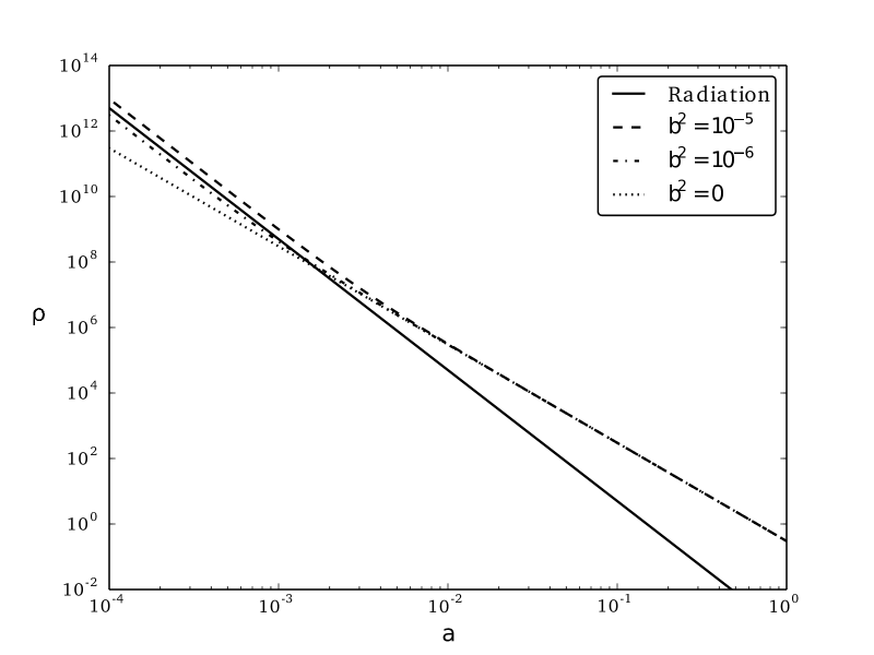
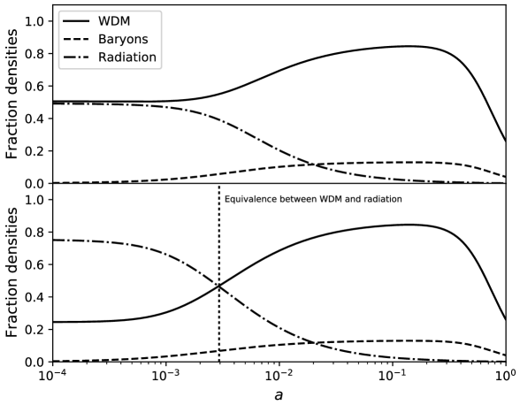
Figure 1: Left panel: Comparison between radiation density and WDM density for several values of $b^{2}$. For the values $b^{2}\gtrsim 10^{-6}$ there is no radiation dominated era and WDM always dominates after inflation. Right panel: Fractional abundances as functions of scale factor for baryons, radiation and WDM for $b^{2}=10^{-5}$ (top) and $b^{2}=10^{-6}$ (bottom).

The early domination of WDM is shown in Fig. 1. The left panel of the Fig. 1 shows the densities of radiation and WDM for different values of parameter $b$. We can see that for $b^{2}$-values higher than $\sim 10^{-6}$ there is no radiation-dominated era. After inflation the universe is always dominated by WDM. Moreover, for any value of $b^{2}$-parameter smaller than $\sim 10^{-6}$, the equality between WDM and radiation happens earlier compared to the CDM case. In the right panel of the Fig. 1 one can see the plot for the scale factor dependence of fractional abundances (i.e. $\Omega_{i}(a)/\Omega_{T}(a)$) for radiation, baryons and WDM (here $\Omega_{T}(a)$ is the total density parameter). The plot in the top panel corresponds to the case $b^{2}=10^{-5}$ and clearly shows that WDM always dominates, while in the bottom panel, for $b^{2}=10^{-6}$, we still have an epoch dominated by standard radiation. In both cases the baryons contribution is subdominant. Consider now the structure formation process, which is strongly dependent on the behavior of WDM both at the background and perturbative level. The dynamics of WDM perturbations has been described in Fabris:2008qg , so we can just write down the main result for the dynamics of WDM perturbations. The energy and momentum balance equation, in Fourier space for each $k$-mode in flat universe lead to following equations:

$$\dot{\delta}_{w}+(1+w)\left(\theta_{w}+\frac{\dot{h}}{2}\right)+3{\cal{H}}\left(c^{2}_{s}-w\right)\delta_{w}+9{\cal{H}}^{2}\left(c^{2}_{s}-w\right)(1+w)\frac{\theta_{w}}{k^{2}}+3{\cal{H}}\dot{w}\frac{\theta_{w}}{k^{2}}\ =0\,,$$ (10)

$$\dot{\theta}_{w}+{\cal{H}}(1-3c^{2}_{s})\theta_{w}-\frac{k^{2}c^{2}_{s}}{1+w}\delta_{w}=0\,.$$ (11)

For the sake of convenience we used synchronous gauge and hence $h$ is the trace of the scalar metric perturbations, $\delta_{w}\equiv\delta\rho_{w}/\rho_{w}$ is the WDM density contrast and $\theta_{w}$ is the velocity. We have followed conventions for metric signature and Fourier transform of Ma:1995ey , and the dot represents derivative with respect to conformal time $\eta$ and ${\cal{H}}=\dot{a}/a$. Note that for $w=0$, CDM case is reproduced in the above equations. The equations are written in the frame which is co-moving to the WDM fluid and hence here was considered the rest-frame sound speed $c^{2}_{s}$ Weller:2003hw ; Gordon:2004ez . We shall consider WDM as adiabatic fluid. Actually, as far as we are dealing with thermal systems, it is possible that some intrinsic non-adiabaticity traces could be present. However, as a first approximation, we suppose that they are negligible. Then one can use the relation

$$\delta p_{w}=c^{2}_{s}\delta\rho_{w},$$ (12)

where $c^{2}_{s}=\dot{p}_{w}/\dot{\rho}_{w}$. Eqs. (10) and (11) require analytical expression for the rest-frame sound speed and the derivative of the state parameter with respect to the conformal time. Using the background quantities it is straightforward to obtain,

$$\dot{w}=-\frac{{\cal{H}}}{3}\frac{a^{2}}{(a^{2}+b^{2})}\quad\mbox{ and }\quad c^{2}_{s}=w-\frac{\dot{w}}{3{\cal{H}}(1+w)}\,.$$ (13)

In order to solve the system it is necessary to fix initial conditions. The WDM initial conditions can be implemented in the super-horizon regime and deep into the radiation-dominated epoch, i.e., $a\propto\eta$. In the fluid description, for the early radiation era, WDM case can be described by the following equations:

$$\dot{\delta}_{w}+\frac{4}{3}\theta_{w}+\frac{2}{3}\dot{h}=0\qquad\mbox{ and }\qquad\dot{\theta}_{w}-\frac{k^{2}}{4}\delta_{w}=0\,.$$ (14)

By solving equation for $h$ in the super-horizon limit and in the radiation era we arrive to the well-known solution $h\propto(k\eta)^{2}$. With the last solution we found, for the relevant limits, that $\delta_{w}=-\frac{2}{3}C(k\eta)^{2}$ and $\theta_{w}=-\frac{1}{18}Ck(k\eta)^{3}$ are appropriate initial conditions. Of course, equations (10) and (11) are coupled with DE via background solutions and with baryons and radiation both at the background and perturbative level. One has to solve the complete system in order to analyse the consequences of DM warmness for the observables such as, e.g., CMB power spectrum, linear matter power spectrum and the transfer function.

III Consequences of DM warmness via RRG

In addition to Eqs. (10) and (11) we need also the equations describing perturbations for baryons and radiation. These equations can be found for example in Ma:1995ey and we will not repeat them here. To integrate the system including baryons, radiation, WDM and cosmological constant, we modify the Boltzmann CAMB code Lewis:1999bs . The initial value $\Omega_{b0}=0.0223h^{-2}$ is chosen to provide the agreement with Big Bang nucleosynthesis Pettini:2012ph , while $\Omega_{r0}$ is taken to agree with CMB measurements Ade:2015xua . The free parameters related to WDM are $H_{0}$, $\Omega_{w0}$ and $b$, and in principle they have as priors $0<H_{0}<100$, $0<\Omega_{w0}<1$ and $0<b^{2}\lesssim 10^{-6}$ to ensure a radiation dominated era. In this way we consider a reduction of this WDM space of parameters by using background observational tests. Thus, in what follows we limit our analysis to the values of WDM parameters such that they are in $1\sigma$ CL (confidence level) region of the joint analysis based on SNIa, BAO and $H(z)$ data. This shall help us to get more realistic and measurable warmness effects that do not contradict observations, at least at the background level.

III.1 Background tests

The background tests related to SNIa, BAO and $H_{0}$ are based on the likelihood computed using the $\chi^{2}$ function,

$$\chi^{2}(\theta)=\Delta y(\theta)^{T}\mathbf{C}^{-1}\Delta y(\theta),$$ (15)

where $\theta=(H_{0},\Omega_{m0},b)$ and $\Delta y(\theta)=y_{i}-y(x_{i};\theta)$. Here $y(x_{i};\theta)$ represents the theoretical predictions for a given set of parameters, $y_{i}$ the data and $\mathbf{C}$ is the covariance matrix. Note that, for convenience, the total matter density parameter $\Omega_{m0}=\Omega_{w0}+\Omega_{b0}$ was used here as a free parameter instead of $\Omega_{w0}$.

In order to perform the background statistical analysis it was used the numerical code CLASS Blas:2011rf combined with the statistical code MontePython Audren:2012wb . For the data set we have used the complete SNeIa data and correlation matrix from the JLA sample Betoule:2014frx , $H_{0}$ is considered from Riess:2011yx , and for BAO test we have used data from 6dFGSBeutler:2011hx , SDSS Anderson:2013zyy , BOSS CMASS Padmanabhan:2012hf and WiggleZ survey Kazin:2014qga . The 6dFGS, SDSS and BOSS CMASS data are mutually uncorrelated and also they are not correlated with WiggleZ data, however we must take into account correlation beetween WiggleZ data points given in Kazin:2014qga . The set of free parameters $\theta$ can be divided in two parts: the cosmological free parameters $\Omega_{m0}$, $h$ and $b$; and the nuissance parameters $\alpha$, $\beta$, $M$ and $\Delta_{M}$, related to SNe Ia data. The results of the complete statistical analysis is presented in TABLE 1 and the contour curves are presented in FIG. 2. These results are in agreement with the previous results Fabris:2008qg ; Fabris:2011am but here we have updated the results and error was reduced due to the improved quality of observational data in recent years.

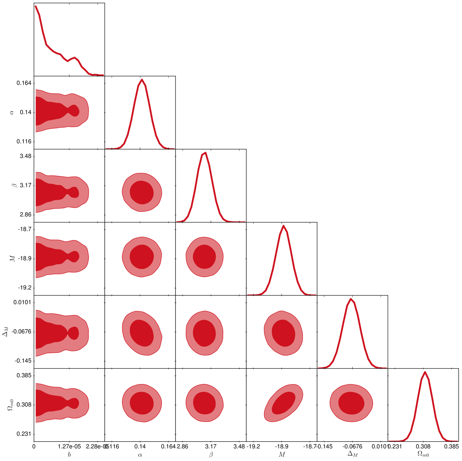
Figure 2: 1$\sigma$ and 2$\sigma$ C.L. curves for the joint analysis using SNIa (JLA), $H_{0}$ and BAO data sets.

Table 1: Result of the statistical analysis for the joint analysis using SNIa (JLA), $H_{0}(z)$ and BAO data sets. The best-fit result was obtained when $\chi_{min}^{2}=685.3$.

Parameter	Best-fit	95% lower	95% upper
$h$	$0.7386$	$0.6923$	$0.7833$
$\Omega_{w0}$	$0.2607$	$0.2237$	$0.3025$
$b$	$6.425\times 10^{-6}$	$0^{*}$	$2.163\times 10^{-5}$
$\alpha$	$0.1417$	$0.1277$	$0.1545$
$\beta$	$3.094$	$2.936$	$3.265$
$M$	$-18.92$	$-19.08$	$-18.78$
$\Delta_{M}$	$-0.07238$	$-0.1181$	$-0.02448$
$\Omega_{m0}$	$0.3107$	$0.2737$	$0.3525$

III.2 Perturbative analysis

The reduced space of parameters is in agreement with the SNIa+BAO+$H(z)$ data, which we will use to study consequences of the DM warmness in the two relevant observables, namely the structure formation and CMB anisotopies. Before starting the coprresponding consideration, let us illustrate the consequences of the free-streaming of WDM in the matter perturbations.

Concerning the structure formation, a relevan quantity is the total matter density contrast,

$$\delta_{m}\equiv\frac{\delta\rho_{m}}{\rho_{m}}=\frac{\delta\rho_{w}+\delta\rho_{b}}{\rho_{w}+\rho_{b}}.$$ (16)

By recalling that for each component $\delta\rho_{x}=\rho_{x}\,\delta_{x}$, one can write analytic expression for the total matter density contrast in the RRG-based model,

$$\delta_{m}=\frac{\tilde{\Omega}_{w}(a)\,\delta_{w}+\Omega_{b0}\,\delta_{b}}{\tilde{\Omega}_{w}(a)+\Omega_{b0}},\qquad\tilde{\Omega}_{w0}(a)=\Omega_{w0}\sqrt{\frac{1+b^{2}\,a^{-2}}{1+b^{2}}}\,.$$ (17)

Let us note that in this case, different from $\Lambda$CDM, the total matter density contrast depends on the scale factor. Furthermore, after decoupling, the contribution of warm matter to total matter density varies from $\sim 100\%$ for $a\ll 1$ ($\delta_{m}\approx\delta_{w}$) to $\sim 87\%$ when $a=1$ (i.e $\delta_{m}\approx 0.87\delta_{w}+0.13\delta_{b}$) while in $\Lambda$CDM the contribution is always constant and of the order $\sim 85\%$ (i.e $\delta_{m}\approx 0.85\delta_{w}+0.15\delta_{b}$).

The left panel of the FIG. 3 shows the total matter density contrast for different scales and for $b^{2}=10^{-14}$. In the top panel it is shown $\delta_{m}$ for scale $k=2hMpc^{-1}$ and in the bottom panel it is shown $\delta_{m}$ for scale $k=5hMpc^{-1}$. In the first case the difference with CDM case is minimal and $\sim 5\%$ at maximum. However, in the second case, this difference goes to $\sim 20\%$. These results indicate a strong suppression of the growth of matter perturbations at the small scales, in contrast with the CDM case. Once again, one can see that the RRG enables one to reproduce known features of WDM in a very economic way.

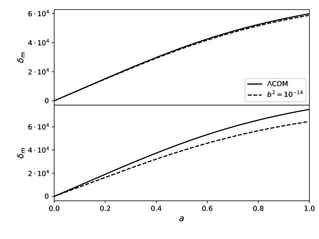
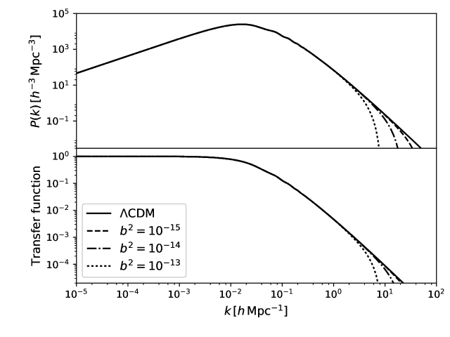
Figure 3: Top left panel: total matter overdensity for $b=10^{-14}$ at scale $k=2hMpc^{-1}$. Maximum difference between WDM and CDM case is $\sim 5\%$), bottom left panel represents the case for $k=5hMpc^{-1}$, where difference to the CDM case is $\sim 20\%$. Top right panel: linear matter power spectrum and bottom right panel: transfer function for different $b$-values. Note that suppression in small scales is proportional to $b$ and is more evident in these quantities.

One should expect that the suppression in the total matter density contrast caused by DM warmness also appears in the linear matter power spectrum and in its transfer function. The linear matter power spectrum is computed as $P(k)\propto k^{n_{s}}T(k)^{2}$, where $n_{s}$ is the scalar spectral index and $T(k)$ is the transfer function. The transfer function is defined as

$$T(k)\equiv\frac{\delta_{m}(k,z=0)\,\delta_{m}(0,z=0)}{\delta_{m}(k,z\rightarrow\infty)\,\delta_{m}(0,z\rightarrow\infty)}\,.$$ (18)

At the next stage we use our modified CAMB code to compute the linear matter power spectrum and transfer function. The results for $b^{2}=10^{-13},10^{-14}$ and $10^{-15}$ are shown in the right panel of the FIG. 3. The top right panel shows the linear matter power spectrum while bottom right panel shows the transfer function for these cases. From these plots one can conclude that at large scales there is no much deviation from the $\Lambda$CDM result, while at the small scales there is considerably lack of power proportional to the value of warmness $b$ in relation to the $\Lambda$CDM. This situation by itself is not new at all, it is regarded as one of the main features of WDM models. However, it is remarkable that one can reproduce it by using the simple RRG description, in a model-independent way and without any supposition about particle physics models.

One can wonder how CMB power spectrum is affected by the suppression on matter overdensities in small scales. The FIG. 4 shows the CMB temperature power spectrum for different $b$-values . One can observe that even with the strong suppression in $P(k)$, the CMB temperature power spectrum is not considerably affected for $b^{2}\lesssim 10^{-10}$. At large scales, when $l\lesssim 30$, all curves coincide. The differences only appear at the scales smaller than $l\sim 30$. The most of the difference is at the intermediate scales $30\lesssim l\lesssim 1300$. In order to quantify deviations from $\Lambda$CDM we compute difference

$$\Delta D_{l}=D^{\Lambda CDM}_{l}-D^{\Lambda WDM}_{l}\,,\qquad D_{l}=\frac{l(l+1)C_{l}}{2\pi}$$ (19)

where $C_{l}$ represents the CMB temperature power spectrum. Bottom panel of Fig. 4 shows $\Delta D_{l}$. Notice that the maximum difference is $\lesssim 0.015\%$ and takes place for $b^{2}=10^{-10}$. However, $\Delta D_{l}$ could be slightly higher for the values of $b$ larger than $b^{2}=10^{-10}$. Even though large scales $l\lesssim 30$ are not influenced by thermal velocities of dark matter, the rest of the spectrum does. It is possible to show that some velocities $\gtrsim 30km/s$ ($b^{2}\gtrsim 10^{-8}$) produce strong distortions in the interval $30\lesssim l\lesssim 1300$, such that it would hardly fit the data.

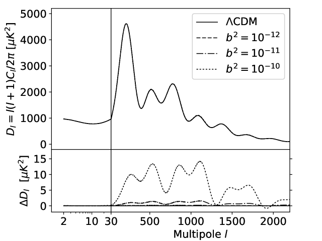
Figure 4: CMB temperature power spectrum for several values of $b$. Plots for $b^{2}=10^{-10},10^{-11}$ and $10^{-12}$ are shown in top panel. In bottom panel it is shown the difference $D_{l}$ defined in eq.(19). Note that for $l\lesssim 30$ all curves are indistinguishable and differences appear after $l\sim 30$. For velocities of the order of $v\lesssim 3km/s$, differences with CDM case is $\sim 0,015\%$ at maximum.

It is interesting to compare the RRG-based results with the ones which are based on different approaches. In the context of WDM, the effect of the free-streaming on matter distribution is quantified by a relative function transfer $\bar{T}(k)$ which is defined as

$$\bar{T}(k)\equiv\left[\frac{P_{\Lambda\rm{WDM}}(k)}{P_{\Lambda\rm{CDM}}(k)}\right]^{1/2},$$ (20)

where $\,P_{\Lambda\rm{WDM}}\,$ and $\,P_{\Lambda\rm{CDM}}\,$ are linear matter power spectra for $\Lambda\rm{WDM}$ and $\Lambda\rm{CDM}$ cases, respectively. The function $\bar{T}(k)$ can be approximated by the following fitting expression Bode:2000gq ,

$$\bar{T}(k)=[1+(\alpha k)^{2\nu}]^{-5/\nu},$$ (21)

where $\alpha$ and $\nu$ are fitting parameters.

For the sake of comparison, let us denote the relative function transfer computed via RRG by $\bar{T}_{RRG}(k)$. After computing $\bar{T}_{RRG}(k)$, we perform a fit for Eq. (21) and find parameters $\alpha$ and $\nu$ for different values of $b$. The results are summarized in three first entries of Table II. The results show that RRG reproduces the relative transfer function which is considered standard in the WDM framework with accuracy of $\lesssim 1\%$, which can be seen in FIG. 5.

In the left top panel of FIG. 5 we show $\bar{T}_{RRG}(k)$ with $b^{2}=10^{-15}$ and $\bar{T}(k)$ with $\alpha=0.0147$ and $\nu=1.12$, and in its bottom panel it is shown the relative error between $\bar{T}_{RRG}(k)$ and $\bar{T}(k)$. The same plots are shown in right panel of FIG. 5 for the case where the $\bar{T}_{RRG}(k)$ was computed with $b^{2}=10^{-14}$ and $\bar{T}(k)$ was computed with $\alpha=0.0242$ and $\nu=1.12$. Note that, for both cases, the relative error is $\lesssim 1\%$.

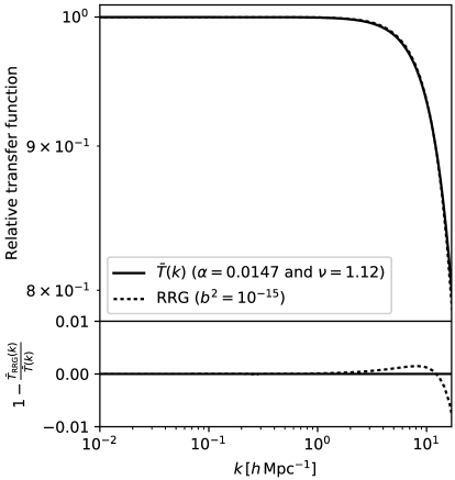
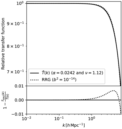
Figure 5: Top left: Plots for $\bar{T}_{RRG}(k)$ with $b^{2}=10^{-15}$ and $\bar{T}(k)$ with $\alpha=0.0147$ and $\nu=1.12$. Top right: $\bar{T}_{RRG}(k)$ with $b^{2}=10^{-14}$ and $\bar{T}(k)$ with $\alpha=0.0242$ and $\nu=1.12$. Bottom left and right: relative error for both cases.

In what follows we shall consider a more detailed comparison between RRG approach and the well established particle physics candidate for WDM associated to thermal relics. Our comparison shall include some non-linear features.

Table 2: Result of the statistical analysis for the joint analysis using SNIa (JLA), $H_{0}(z)$ and BAO data sets. The best-fit result was obtained when $\chi_{min}^{2}=685.3$.

$b^{2}$	$\alpha$	$\nu$
$10^{-10}$	$2.450$	$2.12$
$10^{-11}$	$0.510$	$1.64$
$10^{-12}$	$0.350$	$1.23$
$10^{-13}$	$0.092$	$1.15$
$10^{-14}$	$0.028$	$1.10$
$10^{-15}$	$0.005$	$0.92$

IV Thermal relics via RRG

In the context of thermal relics it is well-known that there is a lower bound of $3.3\,keV$ for the WDM particle mass. Hence it would be interesting to perform a comparison between thermal relics with such a bound and RRG approach. For this reason, it is necessary first to find a equivalence between thermal relics mass scales and RRG $b$-parameter. Thus we recall that for relics we have $\nu=1.12$ and the parameter $\alpha$, in units of $h^{-1}\rm{Mpc}$, is related to the mass scale $m_{w}$ via Viel:2005qj ; Bode:2000gq ; Hansen:2001zv ,

$$\alpha=0.049\left(\frac{m_{w}}{1keV}\right)^{-1.11}\left(\frac{\Omega_{w0}}{0.25}\right)^{0.11}\left(\frac{0.01H_{0}}{0.7}\right)^{1.22}\,.$$ (22)

In order to obtain a complete association of the RRG parameter $b^{2}$ and the mass of WDM particles in the thermal relics context, it was used the following particular set of values for the $b^{2}$,

$$b^{2}=\left(1\times 10^{-15},2\times 10^{-15},\,\ldots\,,9\times 10^{-12},1\times 10^{-11}\right)\,.$$ (23)

For each point it was defined a $\chi^{2}$ function,

$$\chi^{2}=\left(\bar{T}\left(k\right)^{th.}-\bar{T}\left(k\right)^{num.}\right)^{2}\,,$$ (24)

where the $\bar{T}\left(k\right)^{th.}$ is given by the equation (21) and the $\bar{T}\left(k\right)^{num.}$ is obtained with the CAMB code for each value of $b^{2}$ in the set (23). Then we minimize the equation (24) in order to find the best-fit $\alpha$-value for each $b^{2}$.

Using the equation (22) we found, for each value of $b^{2}$, the corresponding mass $m_{w}$. This correspondence is shown in FIG. 6, where the dots indicate the best-fit value for $m_{w}$ found through the equation (24) and the solid line is the linear regression in the loglog frame. This linear regression results in the following fit-formula,

$$m_{w}=4.65\cdot 10^{-6}\,\left(b^{2}\right)^{-2/5}keV.$$ (25)

By using eq.(25) we found that a mass scale of $3.3\,keV$ in thermal relics is equivalent to $b^{2}=2.36\times 10^{-15}\sim 10^{-15}$ in RRG approach. This value for $b^{2}$ brings difficulties in distinguishing between WDM and CDM scenarios both at background and linear level. At background this can be seen in the left panel of the FIG. 1, where for $b^{2}\lesssim 10^{-6}$ the expansion dynamics after matter-radiation equality is indistinguishable from CDM case and also, the best fit value for $\Omega_{m0}$ is almost the same as $\Lambda$CDM (see FIG. 2). On the other hand, at linear regime, CMB signal via RRG for $b^{2}\lesssim 10^{-10}$ is completly indistinguishable of $\Lambda$CDM (see FIG. 4) and linear matter power spectrum has the expected little suppreession in small scales (see FIG. 3). In order to better observe such tiny differences, we can for example, recompute the matter power spectrum in the Fourier space in its dimensionless form, denoted by $\Delta^{2}\left(k\right)=\frac{k^{3}}{2\pi^{2}}P(k)$ .

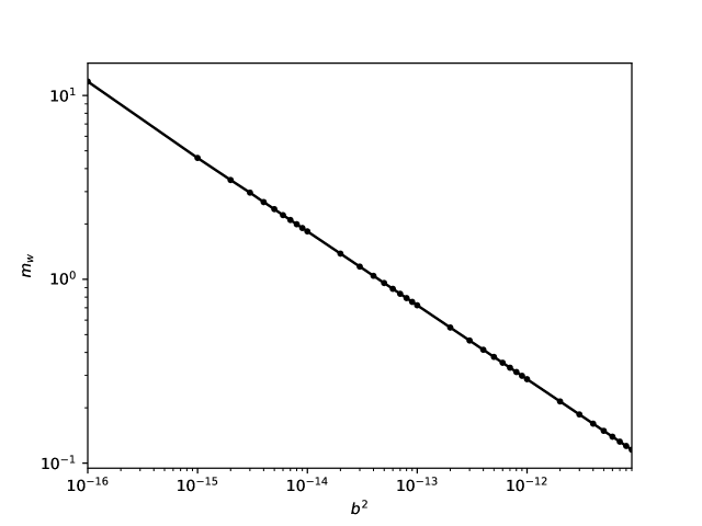
Figure 6: Fitting formula for the WDM mass particle (in $keV$) in terms of the RRG parameter $b^{2}$.

The left panel of the FIG. 7 shows $\Delta^{2}(k)$ at $z=0$ for both cases: standard treatment for thermal relics with mass $3.3\,keV$ and thermal relics via RRG approach with $b^{2}=10^{-15}$. We can see that CDM and WDM (thermal relics) are indistinguishable until $\Delta^{2}\left(k\right)\sim 30$ where $\Delta^{2}\left(k\right)$ falls off too rapidly. In fact, in the context of thermal-like candidates, this feature has been used as justification to claim that albeit such a cut-off is still consistent with constraints based on Lyman-$\alpha$ forest data, for masses larger than 3.3 $keV$, the WDM appears no better than CDM in solving the small scale anomalies Schneider:2013wwa . Of course, this affirmation needs to be better investigated in the context of others WDM candidates and, if possible, in a model-independent way. Thus, we believe that RRG can be very helpful in such direction.

On the other hand, we can also compute the time scale where the perturbations reach the non-linear regime. In the right panel of the FIG. 7 it is shown the time (redshift) scale $z_{nl}$ in which the matter perturbation scale $R$ reachs the non-linear regime. $z_{nl}$ is the redshift where $\sigma^{2}(R)=1$, being $\sigma^{2}(R)$ the mass variance at the scale $R$. Again both cases are considered: standard treatment for thermal relics with mass $3.3\,keV$ and thermal relics via RRG approach with $b^{2}=10^{-15}$. We can see that, in WDM thermal-like candidates context, the non-linearity is reached more recently than in $\Lambda$CDM for scales $R\lesssim 1\,Mpc\,\,h^{-1}$.

Finally, by using $\Delta^{2}\left(k\right)$, $z_{nl}$ and a top-hat filter normalized with the results from Planck Ade:2015xua it is possible to obtain the density of halos. This quantity gives us the number of collapsed objects above a given mass $M$. Here, the mass function was computed using the method of Sheth:2001dp . In FIG. 8, the mass function obtained following the RRG approach is compared with the one computed for thermal relics in the standard way and with CDM case. Clearly in WDM context, there is less collapsed objetcs than in $\Lambda$CDM. Furthermore, from FIGS. 7 and 8 it is possible to see the huge similarity between the RRG approach and the WDM thermal-like standard description also in the non-linear regime. In fact, the relative error in both cases is $\lesssim 1\%$.

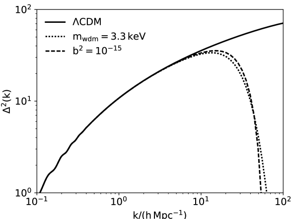
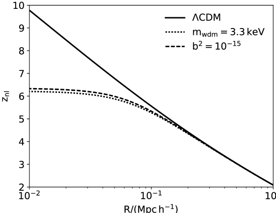
Figure 7: Left panel: Total matter perturbation in the Fourier space. Right panel: Redshift where the matter perturbation reach the non-linear regime in function of the scale. In both cases the solid line corresponds to $\Lambda$CDM model, the dashed line corresponds to the RRG approach and the dotted line corresponds to WDM case (thermal relics) with mass $3.3\,keV$.

Our results in this and in the previous section indicate that RRG approach is good enough to capture important features of WDM in linear regime. Specially the suppression on small scales structures and lack of power in matter spectrum at such scales. Also, in the particular case of thermal relics, RRG reproduces with high precision, the potentialities and weakness of the candidate in both linear and non linear regime. Thus, RRG approach could be considered as a complementary alternative approach to investigate warm matter and specially for understanding general behavior of the WDM scenario in a model-independent way.

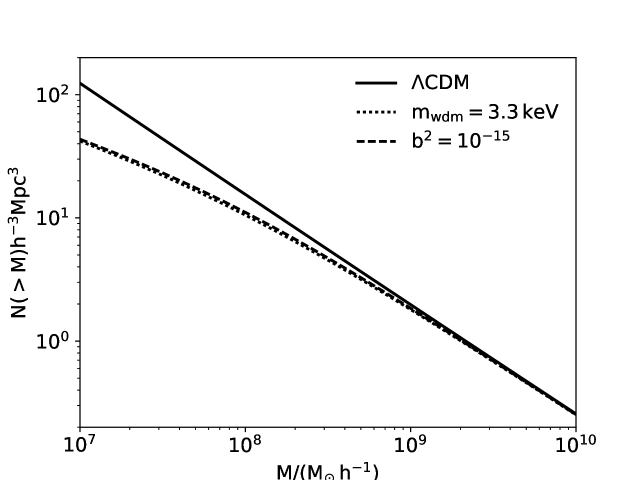
Figure 8: Mass function. The solid line corresponds to $\Lambda$CDM model, the dashed line corresponds to the RRG approach and the dotted line corresponds to standard approach case with mass $3.3\,keV$.

V Discussion and conclusions

We have shown that the RRG approach enable one to model WDM, which is treated as a gas of particles with non-negligible thermal velocities. The simplifying aspect of RRG is that all such velocities are taken to be equal. The presence of warmness produce consequences on the dynamics of the universe both for the background and perturbations.

For the background the most important is that radiation era may be smearing out for greater warmness. In this case the universe is dominated by WDM up to the DE dominated era. This scenario could have deep impact on the primordial nucleosynthesis, reionization, recombination and other effects in the early universe. This new non-standard scenario may be deserving more careful and specific investigation, which we leave for the future work. Our analysis here was limited by the relatively small warmness, with $b^{2}\lesssim 10^{-6}$. In this case the radiation dominated era is still maintained, but the radiation-matter equality takes place before than in the CDM models. After the equality point, there are no serious differences with expansion is dominated by cold matter, as it is shown at the left panel of FIG. 1.

Instead of dealing with the full space of the WDM parameters, we restrict consideration to a more reduced set. At the background level this is achieved by using recent data from SNIa, $H_{0}$ and BAO. As a result we arrive at reduced space which does not contradict more recent background observations at $1\sigma$ CL, i.e $b\in[0,2.1\times 10^{-5}]$ and $\Omega_{m0}=[0.27,0.35]$. Taking this into account one can expect that the quantification of imprint of warmness on observables should become more significant. Our analysis in this reduced space of parameters shows that velocities which satisfy $\nu\lesssim 3\,km/s$ would agree with the CMB observations. This limit is essentially smaller than the bound for HDM, which may have velocities which are just two order of magnitude smaller than the speed of light. The velocities bound which were found here agree with the ones found earlier by other approaches Bond:1983hb ; Hannestad:2000gt ; Viel:2005qj ; Bode:2000gq ; Barkana:2001gr . This fact shows that, regardless of that the RRG is technically simple, it is a sufficiently reliable approach to probe new physics within the WDM approach.

The consequences of a warmness of DM are is more evident in the dynamics of cosmic perturbations. Since DM is supposed to be the main source of forming gravity potentials and overdensities, the impact of the DM warmness on structure formation and CMB anisotropies is evident. In the case of WDM thermal velocities cause free-streaming out from overdense regions, delaying and inhibiting the growth of fluctuations at certain scales. Another way to interpret this effect is by relating velocity to pressure. The non-negligible pressure of WDM, together with the radiation pressure, are resisting the gravitational compression and therefore suppress the power. This effect is stronger in small scales, as can be seen in Fig. 3. Furthermore, from Fig. 4 one can conclude that thermal velocities do not affect considerably the CMB temperature power spectrum for $b\lesssim 10^{-10}$. Indeed, the situation can be opposite for sufficiently large values of $b$.

As a next step we reproduced features of thermal relics by using RRG prescription. First it was necessary to find a relation between the mass scale in relics context and the $b^{2}$ parameter of RRG. The $b^{2}\sim 10^{-15}$ equivalent to the lower bound known for thermal relics ($3.3keV$) brings the necessity to look more carefully matter perturbations. Thus, we computed the matter perturbations in the Fourier space $\Delta^{2}(k)$, the time scale where the perturbations reach the non-linear regime ($z_{nl}$) and the mass function. In all those cases, our results indicate that RRG approach is good enough to capture important features of WDM even in non-linear regime. Therefore, we have proved that RRG is a reliable model, and can be considered as a complementary, greatly simplified alternative approach to investigate warm matter, in particular for understanding the behavior of the WDM in a totally model-independent way.

One can foresee the possibility of detailed investigations of the new Particle Physics candidates to WDM, which includes the comparison with model-independent RRG. In our opinion some aspects of this possibility would be quite interesting. For example, let us mention a relation between $\bar{T}_{RRG}(k)$ and WDM candidate models, a more complete and comprehensive exploration of the space of parameters via Markov Chain Monte Carlo (MCMC) or verifying how RRG would work in the nonlinear regime of structure formation through numerical simulations and the possibility if WDM is really capable of solve small scale problems. The work on these aspects of the model is currently in progress.

References

- (1) A. G. Riess et al., “Observational evidence from supernovae for an accelerating universe and a cosmological constant,” Astron. J., vol. 116, pp. 1009–1038, 1998.
- (2) S. Perlmutter et al., “Measurements of Omega and Lambda from 42 high redshift supernovae,” Astrophys. J., vol. 517, pp. 565–586, 1999.
- (3) M. Tegmark et al., “The 3-D power spectrum of galaxies from the SDSS,” Astrophys. J., vol. 606, pp. 702–740, 2004.
- (4) N. Aghanim et al., “Planck 2015 results. XI. CMB power spectra, likelihoods, and robustness of parameters,” Astron. Astrophys., vol. 594, p. A11, 2016.
- (5) P. A. R. Ade et al., “Planck 2015 results. XIII. Cosmological parameters,” Astron. Astrophys., vol. 594, p. A13, 2016.
- (6) M. Moresco et al., “Improved constraints on the expansion rate of the Universe up to z 1.1 from the spectroscopic evolution of cosmic chronometers,” JCAP, vol. 1208, p. 006, 2012.
- (7) L. Bergström, “Nonbaryonic dark matter: Observational evidence and detection methods,” Rept. Prog. Phys., vol. 63, p. 793, 2000.
- (8) T. Buchert, A. A. Coley, H. Kleinert, B. F. Roukema, and D. L. Wiltshire, “Observational Challenges for the Standard FLRW Model,” Int. J. Mod. Phys., vol. D25, no. 03, p. 1630007, 2016. [1,622(2017)].
- (9) R. R. Caldwell, R. Dave, and P. J. Steinhardt, “Cosmological imprint of an energy component with general equation of state,” Phys. Rev. Lett., vol. 80, pp. 1582–1585, 1998.
- (10) A. R. Liddle and R. J. Scherrer, “A Classification of scalar field potentials with cosmological scaling solutions,” Phys. Rev., vol. D59, p. 023509, 1999.
- (11) P. J. E. Peebles and B. Ratra, “The Cosmological constant and dark energy,” Rev. Mod. Phys., vol. 75, pp. 559–606, 2003.
- (12) V. Sahni and Y. Shtanov, “Brane world models of dark energy,” JCAP, vol. 0311, p. 014, 2003.
- (13) A. Lue, “The phenomenology of dvali-gabadadze-porrati cosmologies,” Phys. Rept., vol. 423, pp. 1–48, 2006.
- (14) A. Yu. Kamenshchik, U. Moschella, and V. Pasquier, “An Alternative to quintessence,” Phys. Lett., vol. B511, pp. 265–268, 2001.
- (15) J. C. Fabris, S. V. B. Goncalves, and P. E. de Souza, “Density perturbations in a universe dominated by the Chaplygin gas,” Gen. Rel. Grav., vol. 34, pp. 53–63, 2002.
- (16) N. Bilic, G. B. Tupper, and R. D. Viollier, “Unification of dark matter and dark energy: The Inhomogeneous Chaplygin gas,” Phys. Lett., vol. B535, pp. 17–21, 2002.
- (17) W. S. Hipolito-Ricaldi, H. E. S. Velten, and W. Zimdahl, “Non-adiabatic dark fluid cosmology,” JCAP, vol. 0906, p. 016, 2009.
- (18) W. Zimdahl, H. E. S. Velten, and W. S. Hipolito-Ricaldi, “Viscous dark fluid Universe: a unified model of the dark sector?,” Int. J. Mod. Phys. Conf. Ser., vol. 3, pp. 312–323, 2011.
- (19) R. F. vom Marttens, L. Casarini, W. Zimdahl, W. S. Hipólito-Ricaldi, and D. F. Mota, “Does a generalized Chaplygin gas correctly describe the cosmological dark sector?,” Phys. Dark Univ., vol. 15, pp. 114–124, 2017.
- (20) A. P. Billyard and A. A. Coley, “Interactions in scalar field cosmology,” Phys. Rev., vol. D61, p. 083503, 2000.
- (21) L. Amendola, “Coupled quintessence,” Phys. Rev., vol. D62, p. 043511, 2000.
- (22) L. Lopez Honorez, B. A. Reid, O. Mena, L. Verde, and R. Jimenez, “Coupled dark matter-dark energy in light of near Universe observations,” JCAP, vol. 1009, p. 029, 2010.
- (23) W. Zimdahl, C. Z. Vargas, and W. S. Hipólito-Ricaldi, “Interacting dark energy and transient accelerated expansion,” in Proceedings, 13th Marcel Grossmann Meeting on Recent Developments in Theoretical and Experimental General Relativity, Astrophysics, and Relativistic Field Theories (MG13): Stockholm, Sweden, July 1-7, 2012, pp. 1577–1579, 2015.
- (24) B. Wang, E. Abdalla, F. Atrio-Barandela, and D. Pavon, “Dark Matter and Dark Energy Interactions: Theoretical Challenges, Cosmological Implications and Observational Signatures,” Rept. Prog. Phys., vol. 79, no. 9, p. 096901, 2016.
- (25) A. R. Fuño, W. S. Hipólito-Ricaldi, and W. Zimdahl, “Matter Perturbations in Scaling Cosmology,” Mon. Not. Roy. Astron. Soc., vol. 457, no. 3, pp. 2958–2967, 2016.
- (26) R. F. vom Marttens, W. S. Hipólito-Ricaldi, and W. Zimdahl, “Baryonic matter perturbations in decaying vacuum cosmology,” JCAP, vol. 1408, p. 004, 2014.
- (27) M. S. Warren, K. Abazajian, D. E. Holz, and L. Teodoro, “Precision determination of the mass function of dark matter halos,” Astrophys. J., vol. 646, pp. 881–885, 2006.
- (28) A. A. Klypin, A. V. Kravtsov, O. Valenzuela, and F. Prada, “Where are the missing Galactic satellites?,” Astrophys. J., vol. 522, pp. 82–92, 1999.
- (29) W. J. G. de Blok, “The Core-Cusp Problem,” Adv. Astron., vol. 2010, p. 789293, 2010.
- (30) M. Boylan-Kolchin, J. S. Bullock, and M. Kaplinghat, “Too big to fail? The puzzling darkness of massive Milky Way subhaloes,” Mon. Not. Roy. Astron. Soc., vol. 415, p. L40, 2011.
- (31) J. R. Bond and A. S. Szalay, “The Collisionless Damping of Density Fluctuations in an Expanding Universe,” Astrophys. J., vol. 274, pp. 443–468, 1983.
- (32) S. Hannestad and R. J. Scherrer, “Selfinteracting warm dark matter,” Phys. Rev., vol. D62, p. 043522, 2000.
- (33) M. Viel, J. Lesgourgues, M. G. Haehnelt, S. Matarrese, and A. Riotto, “Constraining warm dark matter candidates including sterile neutrinos and light gravitinos with WMAP and the Lyman-alpha forest,” Phys. Rev., vol. D71, p. 063534, 2005.
- (34) P. Bode, J. P. Ostriker, and N. Turok, “Halo formation in warm dark matter models,” Astrophys. J., vol. 556, pp. 93–107, 2001.
- (35) R. Barkana, Z. Haiman, and J. P. Ostriker, “Constraints on warm dark matter from cosmological reionization,” Astrophys. J., vol. 558, p. 482, 2001.
- (36) C.-P. Ma and E. Bertschinger, “Cosmological perturbation theory in the synchronous and conformal Newtonian gauges,” Astrophys. J., vol. 455, pp. 7–25, 1995.
- (37) A. D. Sakharov, “The initial stage of an expanding Universe and the appearance of a nonuniform distribution of matter,” Sov. Phys. JETP, vol. 22, pp. 241–249, 1966.
- (38) L. P. Grishchuk, “Cosmological Sakharov Oscillations and Quantum Mechanics of the Early Universe,” Usp. Fiz. Nauk, vol. 182, pp. 222–229, 2012. [Phys. Usp.55,210(2012)].
- (39) G. de Berredo-Peixoto, I. L. Shapiro, and F. Sobreira, “Simple cosmological model with relativistic gas,” Mod. Phys. Lett., vol. A20, pp. 2723–2734, 2005.
- (40) F. Juttnerttner Ann. der Phys., vol. Bd 116, p. S. 145, 1911.
- (41) W. Pauli, Theory of relativity. Courier Corporation, 1981.
- (42) J. C. Fabris, I. L. Shapiro, and F. Sobreira, “DM particles: how warm they can be?,” JCAP, vol. 0902, p. 001, 2009.
- (43) L. G. Medeiros, “Cosmological analytic solutions with reduced relativistic gas,” Mod. Phys. Lett., vol. A27, p. 1250194, 2012.
- (44) J. C. Fabris, I. L. Shapiro, and A. M. Velasquez-Toribio, “Testing dark matter warmness and quantity via the reduced relativistic gas model,” Phys. Rev., vol. D85, p. 023506, 2012.
- (45) S. C. d. Reis and I. L. Shapiro, “Cosmic anisotropy with Reduced Relativistic Gas,” 2017.
- (46) J. Weller and A. M. Lewis, “Large scale cosmic microwave background anisotropies and dark energy,” Mon. Not. Roy. Astron. Soc., vol. 346, pp. 987–993, 2003.
- (47) C. Gordon and W. Hu, “A Low CMB quadrupole from dark energy isocurvature perturbations,” Phys. Rev., vol. D70, p. 083003, 2004.
- (48) A. Lewis, A. Challinor, and A. Lasenby, “Efficient computation of CMB anisotropies in closed FRW models,” Astrophys. J., vol. 538, pp. 473–476, 2000.
- (49) M. Pettini and R. Cooke, “A new, precise measurement of the primordial abundance of Deuterium,” Mon. Not. Roy. Astron. Soc., vol. 425, pp. 2477–2486, 2012.
- (50) D. Blas, J. Lesgourgues, and T. Tram, “The Cosmic Linear Anisotropy Solving System (CLASS) II: Approximation schemes,” JCAP, vol. 1107, p. 034, 2011.
- (51) B. Audren, J. Lesgourgues, K. Benabed, and S. Prunet, “Conservative Constraints on Early Cosmology: an illustration of the Monte Python cosmological parameter inference code,” JCAP, vol. 1302, p. 001, 2013.
- (52) M. Betoule et al., “Improved cosmological constraints from a joint analysis of the SDSS-II and SNLS supernova samples,” Astron. Astrophys., vol. 568, p. A22, 2014.
- (53) A. G. Riess, L. Macri, S. Casertano, H. Lampeitl, H. C. Ferguson, A. V. Filippenko, S. W. Jha, W. Li, and R. Chornock, “A 3% Solution: Determination of the Hubble Constant with the Hubble Space Telescope and Wide Field Camera 3,” Astrophys. J., vol. 730, p. 119, 2011. [Erratum: Astrophys. J.732,129(2011)].
- (54) F. Beutler, C. Blake, M. Colless, D. H. Jones, L. Staveley-Smith, L. Campbell, Q. Parker, W. Saunders, and F. Watson, “The 6dF Galaxy Survey: Baryon Acoustic Oscillations and the Local Hubble Constant,” Mon. Not. Roy. Astron. Soc., vol. 416, pp. 3017–3032, 2011.
- (55) L. Anderson et al., “The clustering of galaxies in the SDSS-III Baryon Oscillation Spectroscopic Survey: baryon acoustic oscillations in the Data Releases 10 and 11 Galaxy samples,” Mon. Not. Roy. Astron. Soc., vol. 441, no. 1, pp. 24–62, 2014.
- (56) N. Padmanabhan, X. Xu, D. J. Eisenstein, R. Scalzo, A. J. Cuesta, K. T. Mehta, and E. Kazin, “A 2 per cent distance to =0.35 by reconstructing baryon acoustic oscillations - I. Methods and application to the Sloan Digital Sky Survey,” Mon. Not. Roy. Astron. Soc., vol. 427, no. 3, pp. 2132–2145, 2012.
- (57) E. A. Kazin et al., “The WiggleZ Dark Energy Survey: improved distance measurements to z = 1 with reconstruction of the baryonic acoustic feature,” Mon. Not. Roy. Astron. Soc., vol. 441, no. 4, pp. 3524–3542, 2014.
- (58) M. Viel, G. D. Becker, J. S. Bolton, and M. G. Haehnelt, “Warm dark matter as a solution to the small scale crisis: New constraints from high redshift Lyman-α forest data,” Phys. Rev., vol. D88, p. 043502, 2013.
- (59) S. H. Hansen, J. Lesgourgues, S. Pastor, and J. Silk, “Constraining the window on sterile neutrinos as warm dark matter,” Mon. Not. Roy. Astron. Soc., vol. 333, pp. 544–546, 2002.
- (60) A. Schneider, D. Anderhalden, A. Maccio, and J. Diemand, “Warm dark matter does not do better than cold dark matter in solving small-scale inconsistencies,” Mon. Not. Roy. Astron. Soc., vol. 441, p. 6, 2014.
- (61) R. K. Sheth and G. Tormen, “An Excursion set model of hierarchical clustering : Ellipsoidal collapse and the moving barrier,” Mon. Not. Roy. Astron. Soc., vol. 329, p. 61, 2002.