Parareal Algorithm Implementation and Simulation in Julia

Abstract.

We present a full implementation of the parareal algorithm—an integration technique to solve differential equations in parallel—in the Julia programming language for a fully general, first-order, initial-value problem. We provide a brief overview of Julia—a concurrent programming language for scientific computing. Our implementation of the parareal algorithm accepts both coarse and fine integrators as functional arguments. We use Euler’s method and another Runge-Kutta integration technique as the integrators in our experiments. We also present a simulation of the algorithm for purposes of pedagogy and as a tool for investigating the performance of the algorithm.

1. Introduction

The parareal algorithm was first proposed in 2001 by Lions, Maday, and Turinici (Lions et al., 2001) as an integration technique to solve differential equations in parallel. We present a full implementation of the parareal algorithm in the Julia programming language (https://julialang.org) (Moffit and Tate, 2014) for a fully general, first-order, initial-value problem. Furthermore, we present a simulation of the algorithm for purposes of pedagogy and as a tool for investigating the performance of the algorithm. Our implementation accepts both coarse and fine integrators as functional arguments. We use Euler’s method and another Runge-Kutta integration technique as the integrators in our experiments. We start with a brief introduction to the Julia programming language.

2. An Introduction to Julia: Dynamic, yet Efficient, Scientific/Numerical Programming

Julia is a multi-paradigm language designed for scientific computing; it supports multidimensional arrays, concurrency, and metaprogramming. Due to both Julia’s LLVM-based Just-In-Time compiler and the language design, Julia programs run computationally efficient—approaching and sometimes matching the speed of languages like C. See (web, ) for a graph depicting the relative performance of Julia compared to other common languages for scientific computing on a set of micro-benchmarks.

2.1. Coroutines and Channels in Julia

Coroutines are typically referred to as tasks in Julia, and are not scheduled to run on separate CPU cores. Channels in Julia can be either synchronous or asynchronous, and can be typed. However, if no type is specified in the definition of a channel, then values of any type can be written to that channel, much like unix pipes. Messages are passed between coroutines through channels with the put! and take!() functions. To add tasks to be automatically scheduled, use the schedule() function, or the @schedule and @sync macros. Of course, coroutines have little overhead, but will always run on the same cpu.

The current version of Julia multiplexes all tasks onto a single os thread. Thus, while tasks involving i/o operations benefit from parallel execution, compute bound tasks are effectively executed sequentially on a single os thread. Future versions of Julia may support scheduling of tasks on multiple threads, in which case compute bound tasks will see benefits of parallel execution too(Jul, ).

2.2. Parallel Computing

In addition to tasks, Julia supports parallel computing—functions running on multiple cpus or distributed computers. New processes are spawned with addproc($\mathtt{<}$n$\mathtt{>}$), where $\mathtt{<}$n$\mathtt{>}$ is the number of processes desired. The function addproc returns the pids of the created processes. The function workers returns a list of the processes. Alternatively, the Julia interpreter can be started with the -p $\mathtt{<}$n$\mathtt{>}$ option, where $\mathtt{<}$n$\mathtt{>}$ is the number of processes desired. For instance:

⬇

$ julia

julia> addprocs(3)

3-element Array{Int64,1}:

2

3

4

julia> workers()

3-element Array{Int64,1}:

2

3

4

^D

$

$ julia -p 3

julia> workers()

3-element Array{Int64,1}:

2

3

4

^D

$

Note that the process ids start at 2 because the Julia REPL shell is process 1.

Processes in Julia, which are either locally running or remotely distributed, communicate with each other through message passing.

The function remotecall($\mathtt{<}$Function$\mathtt{>}$, $\mathtt{<}$ProcessID$\mathtt{>}$, $\mathtt{<}$args …$\mathtt{>}$) executes $\mathtt{<}$Function$\mathtt{>}$ on worker $\mathtt{<}$ProcessID$\mathtt{>}$ and returns a value of the Future type, which contains a reference to a location from which the return value can be retrieved, once $\mathtt{<}$Function$\mathtt{>}$ has completed its execution. The Future value can be extracted with the function fetch(), which blocks until the result is available. Thus, the function remotecall is used to send a message while the function fetch is used to receive a message. For instance:

⬇

julia> addprocs(2)

julia> future = remotecall(sqrt, 2, 4)

Future(2,1,3,Nullable{Any}())

julia> fetch(future)

2.0

After the function remotecall is run, the worker process simply waits for the next call to remotecall.

⬇

julia> counter1 = new_counter(3)

(::#1) (generic function with 1 method)

julia> future = remotecall(counter1, 2)

Future(2,1,23,Nullable{Any}())

julia> fetch(future)

4

The Julia macro @spawn simplifies this message-passing protocol for the programmer and obviates the need for explicit use of the low-level remotecall function. Similarly, the macro @parallel can be used to run each iteration of a (for) loop in its own process.

⬇

julia> future = @spawn sqrt(4)

julia> fetch(future)

2.0

julia> addprocs(2)

2-element Array{Int64,1}:

3

4

julia> @everywhere function fib(n)

if (n < 2)

return n

else

return fib(n-1) + fib(n-2)

end

end

julia> @everywhere function fib_parallel(n)

if (n < 35)

return fib(n)

else

x = @spawn fib_parallel(n-1)

y = fib_parallel(n-2)

return fetch(x) + y

end

end

julia> @time fib(42)

2.271563 seconds (793 allocations: 40.718 KB)

267914296

julia> @time fib_parallel(42)

3.483601 seconds (344.48 k allocations:

15.344 MB, 0.25% gc time)

There are also remote channels which are writable for more control over synchronizing processes.

2.3. Multidimensional Arrays

Julia supports multidimensional arrays, an important data structure in scientific computing applications, with a simple syntax and their efficient creation and interpretation over many dimensions (Bezanson et al., 2014). The function call ArrayType($\mathtt{<}$dimensions$\mathtt{>}$) creates an array, where the $n^{\mathrm{th}}$ argument in $\mathtt{<}$dimensions$\mathtt{>}$ specifies the size of the $n^{\mathrm{th}}$ dimension of the array. Similarly, the programmer manipulates these arrays using function calls that support infinite-dimensional arrays given only limitations on computational time.

In summary, Julia incorporates concepts and mechanisms—particularly concurrency and multidimensional arrays—which support efficient scientific computing.

3. The Parareal Algorithm

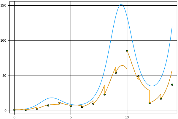
Figure 1. Right endpoint error.

The parareal algorithm is designed to perform parallel-in-time integration for a first-order initial-value problem. The algorithm involves two integration techniques, often known as the ‘coarse’ integrator and the ‘fine’ integrator. For the algorithm to be effective, the coarse integrator must be of substantially lower computational cost than the fine integrator. The reason will become apparent later in this section. Consider the differential equation $\eqref{ode}$ given by

(1) $$y^{\prime}(t)=f(t,y(t))\quad t\in[a,b]$$

with its associated initial-value problem $\eqref{ivp}$

(2) $$y(t^{*})=y^{*}\quad t^{*}\in[a,b]\mathrm{.}$$

For simplicity, let us assume $t^{*}=a$, so that the solution only extends rightward. To obtain an approximate solution to equation $\eqref{ode}$ satisfying the initial condition $\eqref{ivp}$, we partition our domain into $[t_{0}=a,...,t_{N}=b]$ with uniform step size $\Delta$. We now precisely define an ‘integrator’ as a function from $(0,\infty)\times\mathbb{R}^{2}\times\mathscr{R}$ to $\mathbb{R}$ where $\mathscr{R}$ is the set of all Riemann integrable functions. For example, the integrator $I$ given by

$$I(\delta,x_{0},y_{0},g)=y_{0}+g(x_{0},y_{0})\delta$$

is the integrator corresponding to Euler’s method with step size $\delta$. Let $\mathscr{C}$ and $\mathscr{F}$ be the coarse and fine integrators, respectively. Define

$$y_{0,1} =y(t_{0})=y^{*}$$

$$y_{n+1,1} =y(t_{n+1})=\mathscr{C}(\Delta,t_{n},y_{n,1},f)\mathrm{.}$$

Since $y_{n+1,1}$ depends on $y_{n,1}$, this algorithm is inherently sequential. Partition $[t_{n},t_{n+1}]$ into $\{t_{n}^{0}=t_{n},...,t_{n}^{m},...t_{n}^{M}=t_{n+1}\}$ with uniform step size $\delta<\Delta$. Define

$$z_{n,1}^{0} =y(t_{n}^{0})=y_{n,1}$$

$$z_{n,1}^{m+1} =y(t_{n}^{m+1})=\mathscr{F}(\delta,t_{n}^{m},z_{n,1}^{m},f)\mathrm{.}$$

This yields an approximate solution $\{z_{n,1}^{0},...,z_{n,1}^{M}\}$ to $\eqref{ode}$ over $[t_{n},t_{n+1}]$ with initial conditions

$$y(t_{n})=y_{n,1}\mathrm{.}$$

Since $z_{n_{1},1}^{m_{1}}$ does not depend on $z_{n_{2},1}^{m_{2}}$ for $n_{1}\neq n_{2}$, we can compute these approximations in parallel. After the last subproblem is solved, we simply combine the solutions on each subdomain to obtain a solution over the whole interval. However, our values $\{y_{1,1},...,y_{n,1}\}$ are relatively inaccurate. The vertical spikes in the orange graph separating the coarse and fine predictions in Figure 1 illustrate this error. However, $z_{n-1,1}^{M}$ is a better approximation for $\phi(t_{n})$ where $\phi$ is the exact solution to the differential equation. We use this to obtain a better set of points $\{y_{n,2}\}$ for the coarse approximation. We do this by first defining $w_{n,1}=y_{n,1}$ and then defining

$$w_{1,2} =y_{1,1}=y_{1,2}=y^{*}$$

$$w_{n,2} =\mathscr{C}(\Delta,t_{n-1},y_{n-1,2},f)$$

$$y_{n,2} =(w_{n,2}-w_{n,1})+z_{n-1,1}^{M}\mathrm{.}$$

Thus, $w_{n+1,2}$ serves as a new prediction given a more accurate previous prediction from $y_{n,2}$ since $z_{n-1,1}^{M}$ has now been taken into account in calculating $y_{n,2}$. In general, we continue evaluating so that for $k>1$, we have

$$w_{1,k} =y_{1,k}=y^{*}$$

$$w_{n,k} =\mathscr{C}(\Delta,t_{n-1},y_{n-1,k-1},f)$$

$$y_{n,k} =(w_{n,k}-w_{n,k-1})+z_{n-1,k-1}^{M}\mathrm{.}$$

Note that since $y_{n,k}$ is dependent on $w_{n,k}$, this step must be done sequentially. As $k$ increases, $w_{n,k}-w_{n,k-1}\to 0$, which means that $y_{n,k}$ converges to the value that the fine integrator would predict if fine integration were simply done sequentially. Thus, each $k$ denotes fine integration over the whole interval. This means that the total computation performed is much greater than if fine integration were performed sequentially. However, the time efficiency of each iteration has the potential to be improved through concurrency. Since fine integration is more computationally intensive, this improvement in the run-time efficiency may compensate for the cumulative computation performed.

Let $K$ be the total number of iterations necessary to achieve a desired accuracy of solution and $P$ be the number of subintervals into which we divide according to the coarse integrator. If $K=1$, then we achieve perfect parallel efficiency. If $K=P$, then we likely slowed the computation down. The parareal algorithm is guaranteed to converge to the solution given by the sequential fine integrator within $P$ iterations. For a more complete treatment of this convergence analysis, we refer the reader to (Gander and Vandewalle, 2007). For fully general pseudocode, we refer the reader to (Aubanel, 2011; Nielsen, 2012).

4. Parareal Algorithm Implementation in Julia

Listing 1: Implementation of the parareal algorithm in Julia.

⬇

@everywhere function parareal(a,b,nC,nF,K,y0,f,coarseIntegrator,fineIntegrator)

#initialize coarse information

xC = linspace(a,b,nC+1);

yC = zeros(size(xC,1),K);

deltaC = (b-a) / (nC + 1);

yC[1,:] = y0;

#”coarse integrator partially evaluated”

ciPEvaled = ((x1,y1) -> coarseIntegrator(deltaC,x1,y1,f));

#get initial coarse integration solution

for i=2:(nC+1)

yC[i,1] = ciPEvaled(xC[i-1],yC[i-1,1]);

end

correctC = copy(yC);

#initialize fine information

xF = zeros(nC,nF+1);

for i=1:nC

xF[i,:] = linspace(xC[i],xC[i+1],nF+1);

end

sub = zeros(nC,nF+1,K);

deltaF = xF[1,2] - xF[1,1];

#”fine integrator partially evaluated”

fiPEvaled = ((x1,y1) -> fineIntegrator(deltaF,x1,y1,f));

for k=2:K

#run fine integration on each subdomain

tic();

@sync for i=1:nC

sub[i,1,k] = correctC[i,k-1];

@async for j=2:(nF+1)

sub[i,j,k] = fiPEvaled(xF[i,j-1],sub[i,j-1,k]);

end

end

toc();

#predict and correct

for i=1:nC

yC[i+1,k] = ciPEvaled(xC[i],correctC[i,k]);

correctC[i+1,k] = yC[i+1,k] - yC[i+1,k-1] + sub[i,nF+1,k];

end

end

yF = zeros(nC*(nF+1),K-1);

for k=2:K

yF[:,k-1] = reshape(sub[:,:,k]’,nC*(nF+1));

end

return reshape(xF’,nC*(nF+1)),reshape(sub[:,:,K]’,nC*(nF+1)),yF,sub,xC,correctC,yC;

end

Listing 1 presents an implementation of the parareal algorithm (from the prior section) in Julia. The @async macro within the loop causes the program to evaluate the first expression to its right as a concurrent task (i.e., the for loop assigning values to sub). The @sync macro causes the main program thread to wait until all tasks (spawned in the the first expression to its right with an @async or @parallel macro) complete. Once all concurrent tasks are complete, execution of the program proceeds sequentially. Given the semantics of these macros, the program in Listing 1 correctly perform concurrent integration. The sequential and parallel versions of this implementation have no significant differences in run-time efficiency. However, if a sleep statement is placed in the argument of fineIntegrator, the parallel version runs much faster. This demonstrates that use of those two macros does lead to concurrent program execution.

5. Graphical Algorithm Simulation

Listing 2: Implementation of a graphical simulator of the parareal algorithm in Julia.

⬇

@everywhere function fullMethod(n,a,b,y0,f,integrator)

#setup domain and range space

x = linspace(a,b,n+1);

deltaX = x[2] - x[1];

y = ones(n+1,1);

#initialize left endpoint

y[1] = y0;

#integrate each point

for i=1:n

y[i+1] = integrator(deltaX,x[i],y[i],f);

end

return x,y;

end

function simulate(a,b,N,M,K,y0,f,coarseInt,fineInt,showPrev)

x1,y1 = fullMethod(N*(M+1),a,b,y0,f,fineInt);

x,y,yF,sub,xC,yC,iC = parareal(a,b,N,M,K,y0,f,coarseInt,fineInt);

xF = (reshape(x,M+1,N))’;

fine = M+1;

for k=2:K

display(plot(x1,y1));

if(showPrev && k > 2 )

display(scatter!(xC,yC[:,k-2],color=”red”,legend=false));

end

display(scatter!(xC,yC[:,k-1],color=”green”,legend=false));

done = zeros(Int64,N,1);

workingSubdomains = 1:N;

while(done != (M+1) * ones(N,1) )

index = Int64(ceil(size(workingSubdomains,1)*rand()));

currThread = workingSubdomains[index];

while( done[currThread] == M+1 )

currThread = Int64(ceil(N * rand()));

end

currThreadPlot = Int64(ceil(fine*rand()));

totalAdvance = done[currThread] + currThreadPlot;

if(totalAdvance > fine) totalAdvance = fine; end

newP = (done[currThread]+1):totalAdvance;

display(plot!(xF[currThread,newP],sub[currThread,newP,k],color=”black”));

done[currThread] = totalAdvance;

workingSubdomains = find( ((x)->x != M+1), done );

print(join([”Working on subdomain #”, currThread, ”…”,

”Pending Subdomains: ”, workingSubdomains’, ”\n”]));

end

display(plot!(x,yF[:,k-1],color=”orange”));

sleep(5);

end

end

# Implementation schemes.

function euler(delta,x0,y0,f)

return y0 + delta * f(x0,y0);

end

function rungeKutta(delta,x0,y0,f)

k1 = f(x0,y0);

k2 = f(x0+delta/2,y0 + (delta/2)*k1);

k3 = f(x0+delta/2,y0 + (delta/2)*k2);

k4 = f(x0+delta,y0+delta*k3);

return y0 + (delta/6)*(k1+2*k2+2*k3+k4);

end

The function simulate in Listing 2 creates a graphical simulator of the parareal algorithm. This function can be used to introduce the parareal algorithm to students in a numerical analysis course. The first line gets the sequential solution from the fine integrator (the ‘ideal’ solution) and the second line gets the history of the computations that took place during the parareal execution. The main loop over the variable $k$ then displays the inner workings of the algorithm. The ideal solution is plotted, with a scatter plot of the points obtained from the coarse integrator. To simulate the parallel nature of the algorithm, random progress is made on randomly selected subdomains. Thus, the plot dynamically makes partial progress on different subdomains until all subdomains are finished with the fine integration. After this, the plots are connected into the current iteration’s approximation. During the next iteration, the previous guesses from the coarse integrator are displayed in red and the new guesses from the coarse integrator are displayed in green. As $k$ increases, these guesses converge to the ideal solution.

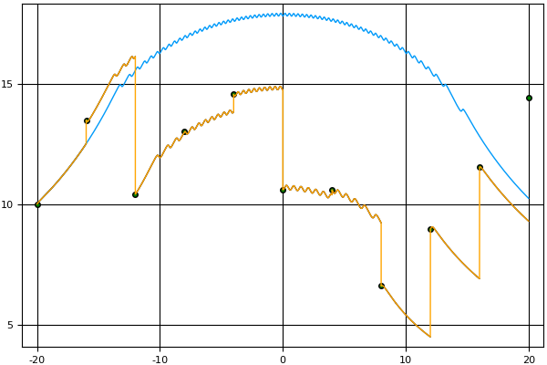
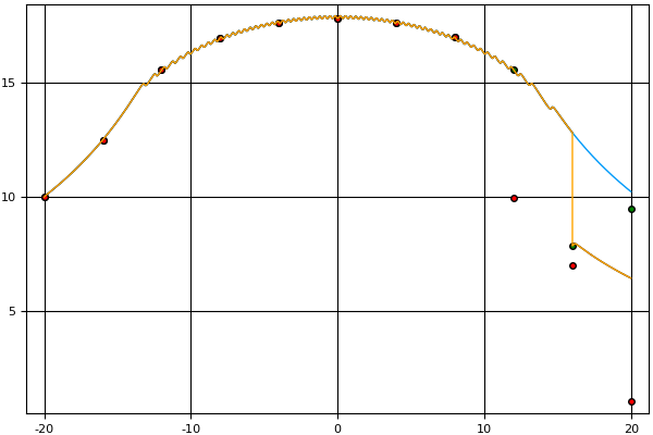
Figure 2. Slow parareal example. (left) Solution after first iteration with Euler’s method. (right) Solution after ninth iteration with Euler’s method.

In addition to the use of this function for pedagogical purposes, it can be used to investigate the types of curves for which the parareal algorithm might be practical. For instance, consider the differential equation

$$y^{\prime}(x)=sin(xy),\quad x\in[-20,20]$$

with $y(-20)=10$, $\Delta=4$ (10 points), and $\delta=0.008$ (500 points). Figure 2 shows the first and ninth iterations. The ninth iteration’s large error on the right end of the interval shows that this is an example where parareal convergence is slow. This is as inefficient as possible, needing as many iterations as subdomains in order for the solution to converge. However, the simulation also shows that if $f(x,y)=sin(x)e^{x}$, then the solution converges after just one iteration. These two examples show that the algorithm’s efficiency can be highly dependent on the integrand. Below the simulation function are Euler’s method and another Runge-Kutta integration technique that can be used as examples to be passed as first-class functions as coarse or fine integration techniques to the ‘parareal’ or ‘simulate’ functions. A Git repository of both the implementation and graphical simulation is available in BitBucket at https://bitbucket.org/sperugin/parareal-implementation-and-simulation-in-julia. All of the graphical plots are generated with the Julia Plots package available at https://juliaplots.github.io/. A video describing this application of Julia is available on YouTube at https://www.youtube.com/watch?v=MtgbeLO6ZM4.

References

- (1)
- (2) Julia Micro-Benchmarks. Available: https://julialang.org/benchmarks/ [Last accessed: 14 November 2018]. (????).
- (3) Julia v1.0 Documentation: Parallel Computing. Available: https://docs.julialang.org/en/v1/manual/parallel-computing/ [Last accessed: 14 November 2018]. (????).
- Aubanel (2011) E. Aubanel. 2011. Scheduling of tasks in the parareal algorithm. Parallel Comput. 37, 3 (2011), 172–182.
- Bezanson et al. (2014) J. Bezanson, J. Chen, S. Karpinski, V. Shah, and A. Edelman. 2014. Array Operators Using Multiple Dispatch: A Design Methodology for Array Implementations in Dynamic Languages. In Proceedings of ACM SIGPLAN International Workshop on Libraries, Languages, and Compilers for Array Programming. ACM Press, New York, NY, 56–61.
- Gander and Vandewalle (2007) M.J. Gander and S. Vandewalle. 2007. Analysis of the parareal time-parallel time-integration method. SIAM Journal on Scientific Computing 29, 2 (2007), 556–578.
- Lions et al. (2001) J.-L. Lions, Y. Maday, and G. Turinici. 2001. A “parareal” in time discretization of PDE’s. Comptes Rendus de l’Académie des Sciences - Series I - Mathematics 332 (2001), 661–668.
- Moffit and Tate (2014) J. Moffit and B.A. Tate. 2014. Julia. In Seven more languages in seven weeks: Languages that are shaping the future, B.A. Tate, F. Daoud, I. Dees, and J. Moffit (Eds.). Pragmatic Bookshelf, Dallas, TX, Chapter 5, 171–207.
- Nielsen (2012) A.S. Nielsen. 2012. Feasibility study of the parareal algorithm. Master’s thesis. Technical University of Denmark.