Pure Natural Inflation

Abstract

We point out that a simple inflationary model in which the axionic inflaton couples to a pure Yang-Mills theory may give the scalar spectral index ($n_{s}$) and tensor-to-scalar ratio ($r$) in complete agreement with the current observational data.

Cosmic inflation plays an important role in explaining observable features of our universe, including its extreme flatness, as well as the origin of primordial curvature perturbations. The detailed predictions of inflation, however, depend on the potential $V(\phi)$ of the inflaton field $\phi$. An important issue, therefore, is to understand what is the correct model of inflation and how it emerges from the underlying physics.

Recent observations by Planck Ade:2015lrj and BICEP2/Keck Array Array:2015xqh have started constraining simple models of inflation. In particular, arguably the simplest model of inflation $V(\phi)=m^{2}\phi^{2}/2$ Linde:1983gd —which gives the correct value for the scalar spectral index $n_{s}\simeq 0.96$—is now excluded at about the $3\sigma$ level because of the non-observation of tensor modes. This raises the following questions. Does the model of inflation need to be significantly complicated? Is the agreement of $n_{s}$ of the quadratic potential with the data purely accidental?

In this letter, we argue that the answers to these questions may both be no. In particular, we argue that a simple inflationary model in which the inflaton $\phi$ couples to the gauge field of a pure Yang-Mills theory

$$\mathcal{L}=\frac{1}{32\pi^{2}}\frac{\phi}{f}\,\epsilon^{\mu\nu\rho\sigma}\,\textrm{Tr}\,F_{\mu\nu}F_{\rho\sigma},$$ (1)

may give the values of $n_{s}$ and the tensor-to-scalar ratio, $r$, in perfect agreement with the current observational data. Here, $\phi$ is a pseudo-Nambu-Goldstone boson—axion—of a shift symmetry $\phi\to\phi+\textrm{const.}$, and $f$ is the axion decay constant. For now we assume that the gauge group of the Yang-Mills theory is $SU(N)$, but the model also works for other gauge groups; see later.

Conventionally, the potential of the axion field as in Eq. (1) is assumed to take the form generated by non-perturbative instantons

$$V(\phi)=\Lambda^{4}\left[1-\cos\left(\frac{\phi}{f}\right)\right],$$ (2)

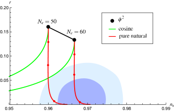
where $\Lambda$ is the dynamical scale of the Yang-Mills theory. The resulting inflation model is called natural inflation Freese:1990rb ; Adams:1992bn , which has been extensively studied in the literature. The potential of Eq. (2), however, is not favored by the current data, and it would soon be excluded at a higher confidence level if the bound on $r$ improves with $n_{s}$ staying at the current value; see Fig. 1.

Figure 1: The predicted values of $n_{s}$ and $r$ superimposed with the $68\%$ and $95\%$ CL BICEP2/KECK Array contours in Ref. Array:2015xqh . The black dots represent the predictions of the quadratic potential $V(\phi)=m^{2}\phi^{2}/2$, with e-folding $N_{e}=50$ and $60$. The green lines are the predictions of the cosine potential, Eq. (2), and the red lines are those of the (holographic) pure natural inflation potential of Eq. (11). For the latter, we have varied $F/M_{\rm Pl}=0.1~{}\mbox{--}~{}100$, with $F/M_{\rm Pl}=10,5,1$ indicated by the red dots (from top to bottom).

It is known since long ago, however, that the cosine potential in Eq. (2) is not correct in general, as argued by Witten Witten:1979vv ; Witten:1980sp in the large $N$ limit tHooft:1973alw with the ’t Hooft coupling $\lambda\equiv g^{2}N$ held fixed. In particular, while the physics is periodic in $\phi$ with the period of $2\pi f$ (because $\theta\equiv\phi/f$ is the $\theta$ angle of the Yang-Mills theory), the multi-valued nature of the potential allows for the potential of $\phi$ in a single branch

$$V(\phi)=N^{2}\Lambda^{4}\,\mathcal{V}\left(\frac{\lambda\phi}{8\pi^{2}Nf}\right),$$ (3)

not to respect the periodicity under $\phi\rightarrow\phi+2\pi f$. Here, the combination

$$x\equiv\frac{\lambda\phi}{8\pi^{2}Nf},$$ (4)

appearing in the argument of $\mathcal{V}(x)$ is determined by analyzing the large $N$ limit. This allows for building axionic models of inflation in which the range of the field excursion exceeds the decay constant $f$ Silverstein:2008sg ; McAllister:2008hb ; Kaloper:2008fb .

The potential of Eq. (3) has an expansion of the form

$$V(\phi)=\sum_{n=1}^{\infty}b_{2n}\left(\frac{\phi}{F}\right)^{2n},$$ (5)

where $F\propto f$. The values of the coefficients $b_{2n}$—more precisely their signs and double ratios—are important for how the predictions for $n_{s}$ and $r$ change as $F$ is varied. If the cosine potential in Eq. (2) were valid, then we would obtain

$$\textrm{sgn}(b_{2n})=(-1)^{n-1},$$ (6)

and

$$\frac{\frac{b_{6}}{b_{4}}}{\frac{b_{4}}{b_{2}}}=\frac{2}{5},\qquad\frac{\frac{b_{8}}{b_{6}}}{\frac{b_{6}}{b_{4}}}=\frac{15}{28},\qquad\cdots,$$ (7)

which lead to the curves labeled as “cosine” in Fig. 1. The correct values of the double ratios, however, are expected to be different from these values. In fact, $b_{2n}$’s obtained by lattice gauge theory disfavor the cosine form of Eq. (2) and are rather consistent with those expected from large $N$ expansion Giusti:2007tu .

While $b_{2n}$’s may in principle be determined by lattice calculations, their errors are still large. Instead, we may infer the form of the potential by the following arguments. First, invariance under the $CP$ transformation $\phi\rightarrow-\phi$ implies that $\mathcal{V}(x)$ is a function of $x^{2}$, where we have absorbed a possible bare $\theta$ parameter in the definition of $\phi$. Second, $\mathcal{V}(x)$ is expected to flatten as the potential energy approaches the point of the deconfining phase transition with increasing $|\phi|$ (since the dynamics generating the potential will become weaker). Assuming that the potential is given by a simple power law, we thus expect $\mathcal{V}(x)\sim 1/(x^{2})^{p}$ ($p>0$). This potential is singular at $x\rightarrow 0$, and a simple way to regulate it is to replace $x^{2}$ with $x^{2}+\textrm{const.}$ After setting the minimum of the potential to be zero, these considerations give

$$V(x)=M^{4}\left[1-\frac{1}{\left(1+cx^{2}\right)^{p}}\right]\quad(p>0),$$ (8)

where $M\sim\sqrt{N}\Lambda$, and $c>0$ is a parameter of order unity. Here, we have used the well-established fact that the coefficient of $x^{2}$ is positive when $\mathcal{V}(x)$ is expanded around $x=0$. We call the model of inflation in which the axionic inflaton potential is generated by a pure Yang-Mills theory (whose potential we expect to take the form of Eq. (8)) pure natural inflation.

As in the cosine potential, the potential of Eq. (8) gives $\textrm{sgn}(b_{2n})=(-1)^{n-1}$. It, however, gives different values of the double ratios

$$\frac{\frac{b_{6}}{b_{4}}}{\frac{b_{4}}{b_{2}}}=\frac{2(p+2)}{3(p+1)},\;\;\cdots,\;\;\frac{\frac{b_{2n+4}}{b_{2n+2}}}{\frac{b_{2n+2}}{b_{2n}}}=\frac{(n+1)(p+n+1)}{(n+2)(p+n)},\;\;\cdots.$$ (9)

Therefore, predictions of this model are different from those of conventional natural inflation. (For example, by equating $(b_{6}/b_{4})/(b_{4}/b_{2})$ we obtain $p=-7/2<0$.) Here, we have assumed that the effect of a transition between different branches can be neglected, which we will argue to be the case.

The potential of Eq. (8) can be obtained by a holographic calculation Dubovsky:2011tu ; Witten:1998uka , which is applicable in the limit of large $N$ and ’t Hooft coupling. In this calculation, $N$ D4-branes in type IIA string theory are considered, with the D4-branes wrapping a circle. Below the Kaluza-Klein scale $M_{\rm KK}$ for the circle, the theory reduces to a 4d (non-supersymmetric) pure $SU(N)$ Yang-Mills theory, with the dynamical scale

$$\Lambda=M_{\rm KK}\,e^{-\frac{24\pi^{2}}{11\lambda}},$$ (10)

where $\lambda$ is the ’t Hooft coupling at $M_{\rm KK}$. Considering the backreaction to the geometry of the constant Wilson line of the Ramond-Ramond one-form, which represents the $\theta$ angle of the gauge theory, the potential of the form of Eq. (8) is obtained with $c=1$ and $p=3$. Specifically, the potential of $\phi$ for a single branch is given by

$$V(\phi)=M^{4}\left[1-\frac{1}{\Bigl{(}1+\bigl{(}\frac{\phi}{F}\bigr{)}^{2}\Bigr{)}^{3}}\right],$$ (11)

where

$$M^{4}=\frac{\lambda N^{2}}{3^{7}\pi^{2}}M_{\rm KK}^{4},\qquad F=\frac{8\pi^{2}N}{\lambda}f.$$ (12)

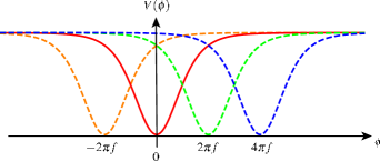
The potentials for the other branches are obtained by replacing $\phi$ with $\phi+2\pi kf$ ($k\in\mathbb{Z}$); see Fig. 2.

Figure 2: The potential of pure natural inflation (in the holographic limit $p=3$); Eq. (11). The potentials for other branches, which ensure the periodicity of physics under $\phi\rightarrow\phi+2\pi f$, are also depicted by dashed lines.

To illustrate the parameter region we consider, let us choose

$$\lambda\simeq 8\pi^{2}.$$ (13)

Strictly speaking, the holographic calculation is not quite valid with this value of the ’t Hooft coupling—it requires a larger value of $\lambda$. However, we may expect, e.g. based on the success of the AdS/QCD program Erlich:2005qh ; DaRold:2005mxj , that this reasonably approximates the true dynamics of the 4d Yang-Mills theory. With this choice of $\lambda$, we find

$$M\approx\sqrt{N}\Lambda,\qquad F\approx Nf,$$ (14)

as one naively expects from dimensional and $N$-scaling considerations. From the analysis of Ref. Dubovsky:2011tu , we expect that for sufficiently large $N$ the effect of a transition between different branches is not important, unless $\phi$ becomes much larger than $F$ (which does not occur in our analysis below). To reproduce the observed amplitude of the scalar perturbation, we will need to take

$$M\sim 10^{16}~{}{\rm GeV}.$$ (15)

The precise value depends on other parameters, e.g. $F$.

The second expression in Eq. (14) implies that for $N\gg 1$ the characteristic scale for the field excursion, $F$, can be much larger than the axion decay constant $f$. This, however, does not mean that $F$ can be much larger than the Planck scale $M_{\rm Pl}\simeq 1.22\times 10^{19}~{}{\rm GeV}$. In general, the decay constant $f$ is expected to be smaller than the field theoretic cutoff (string) scale $M_{*}$

$$f\lesssim M_{*}.$$ (16)

On the other hand, the Planck scale is related with $M_{*}$ as $M_{\rm Pl}^{2}\sim N^{2}M_{*}^{2}$ (see, e.g., Ref. Dvali:2007hz ), so that $N$ drops from the relation between $F$ and $M_{\rm Pl}$:

$$F\lesssim O(M_{\rm Pl}).$$ (17)

We argue that this is a desired feature. If $F\gg M_{\rm Pl}$, the inflaton potential would be well approximated by the first, quadratic term in Eq. (5), which is excluded by the data. Because of Eq. (17), however, we expect that higher terms in Eq. (5) are important. This makes the predictions of the model deviate from those of the quadratic potential $V(\phi)=m^{2}\phi^{2}/2$.

In Fig. 1, we plot the values of $n_{s}$ and $r$ predicted by the potential of Eq. (11). For $F\gg M_{\rm Pl}$, the predictions approach those of the quadratic potential, denoted by the black dots for $e$-folding $N_{e}=50$ (left) and $60$ (right). As $F$ decreases, however, they deviate from these values. In particular, the tensor-to-scalar ratio $r$ decreases while $n_{s}$ being (almost) kept, as represented by the lines indicated as “pure natural.” This is because higher terms in Eq. (5) start contributing. In the figure, we have varied $F$ from $100M_{\rm Pl}$ to $0.1M_{\rm Pl}$, with the predictions for $F/M_{\rm Pl}=10,5,1$ indicated by the red dots (from top to bottom). We find that the model gives the values of $n_{s}$ and $r$ consistent with the data at the $95\%$ ($68\%$) CL for $F/M_{\rm Pl}\lesssim 3.3$ ($0.7$) for $N_{e}=50$ and $F/M_{\rm Pl}\lesssim 6.8$ ($4.4$) for $N_{e}=60$. Given Eq. (17), this is quite satisfactory.

Figure 3: Same as in Fig. 1 but for pure natural inflation potentials with various values of $p=1,2,3,4,10$; see Eq. (18).

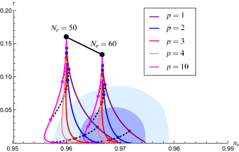
In Fig. 3, we plot the predictions arising from the potential in which $p$ in Eq. (8) takes more general values $p=1,2,3,4,10$. We have parameterized the potentials as

$$V(\phi)=M^{4}\left[1-\frac{1}{\Bigl{(}1+\bigl{(}\frac{\phi}{F}\bigr{)}^{2}\Bigr{)}^{p}}\right],$$ (18)

and, as in Fig. 1, varied $F/M_{\rm Pl}$ in the range between $100$ and $0.1$, with the dots representing $F/M_{\rm Pl}=10,5,1$ (from top to bottom). We find that the success of the model is robust for a wide range of $p\approx 1~{}\mbox{--}~{}O(10)$: the predicted values of $n_{s}$ and $r$ agree well with the current data for $F/M_{\rm Pl}\lesssim O(1)$. We thus conclude that pure natural inflation is consistent with the data even if the true potential does not take exactly the form of Eq. (11) as suggested by the holographic analysis.

So far, we have focused on the case that the gauge group of the Yang-Mills theory is $SU(N)$. However, our basic arguments, e.g. those around Eq. (8), do not depend on this specific choice. We thus expect that similar predictions also result for other gauge groups, with $N$ replaced by the dual Coxeter number of the group.

Finally, we mention that a large value of $N$—despite the fact that it does not help to make $F$ larger than $M_{\rm Pl}$—can make the decay constant $f$ smaller than $F$; see Eq. (14). This allows for enhancing couplings of the inflaton $\phi$ to the standard model gauge fields for fixed $F$, i.e. for a fixed inflation potential. This in turn allows for raising reheating temperature $T_{R}$. The reheating temperature is given by $T_{R}\simeq 0.2\sqrt{\Gamma_{\phi}M_{\rm Pl}}$, where

$$\Gamma_{\phi}\approx\frac{nm_{\phi}^{3}}{4096\pi^{5}f^{2}},$$ (19)

is the inflaton decay width. Here,

$$m_{\phi}=\sqrt{2p}\frac{M^{2}}{F}\simeq\frac{10^{13}~{}{\rm GeV}}{F/M_{\rm Pl}},$$ (20)

is the inflaton mass, and $n$ is the final state multiplicity. ($n=12$ if $\phi$ decays only to the standard model gauge fields.) This yields

$$T_{R}\sim 10^{9}~{}{\rm GeV}\left(\frac{N}{10}\right)\left(\frac{0.5}{F/M_{\rm Pl}}\right)^{5/2},$$ (21)

The model can, therefore, be made consistent with thermal leptogenesis, which requires $T_{R}\gtrsim 2\times 10^{9}~{}{\rm GeV}$ Buchmuller:2005eh , even for $F/M_{\rm Pl}\approx O(1)$.